Optimization of the Operation of Smart Rural Grids through a Novel Energy Management System


Centre d’Innovació Tecnològica en Convertidors Estàtics i Accionaments (CITCEA-UPC), Departament d’Enginyeria Elèctrica, Universitat Politècnica de Catalunya ETS d’Enginyeria Industrial de Barcelona, Av. Diagonal, 647, Pl. 2, 08028 Barcelona, Spain
*
Author to whom correspondence should be addressed.
Energies 2018, 11(1), 9; https://doi.org/10.3390/en11010009
Submission received: 14 November 2017
/
Revised: 16 December 2017
/
Accepted: 18 December 2017
/
Published: 21 December 2017
Abstract
:The paper proposes an innovative Energy Management System (EMS) that optimizes the grid operation based on economic and technical criteria. The EMS inputs the demand and renewable generation forecasts, electricity prices and the status of the distributed storages through the network, and solves with an optimal quarter-hourly dispatch for controllable resources. The performance of the EMS is quantified through diverse proposed metrics. The analyses were based on a real rural grid from the European FP7 project Smart Rural Grid. The performance of the EMS has been evaluated through some scenarios varying the penetration of distributed generation. The obtained results demonstrate that the inclusion of the EMS from both a technical point of view and an economic perspective for the adopted grid is justified. At the technical level, the inclusion of the EMS permits us to significantly increase the power quality in weak and radial networks. At the economic level and from a certain threshold value in renewables’ penetration, the EMS reduces the energy costs for the grid participants, minimizing imports from the external grid and compensating the toll to be paid in the form of the losses incurred by including additional equipment in the network (i.e., distributed storage).
1. Introduction
In the 1990s, the stiff and vertical monopolistic electrical system in Europe experienced a transformation, evolving into a new, more flexible and competitive system based on market aspects [1]. In this new reality the electricity producer decided (and still decides) when and how much to produce, and how to plan and implement their plant maintenance programs [1]. From then on, the traditional unidirectional grid, generally used to carry power from few and far power plants to many clients, is moving to a new modern grid, that integrates scatter and smaller generators throughout the territory. Consequently, modern electric grids combine scatter and smaller generators (even at consumers’ location) with the conventional architecture of the power system [2]. As a result, electrical networks are experiencing bidirectional power flows through distribution grids that impose new challenges for network operation.
To properly manage modern grids, new management strategies for network operators are needed [3,4,5] and the implementation of these management tools are transforming grids into Smart Grids (SGs) [6]. The term energy management was firstly related to those tools managing the demand in grids [7,8,9]. In 1980s the term Demand-Side Management (DSM) was presented by Clark W. Gellings in [7]. The DSM focuses on the idea of influencing customers, through a set of interconnected and flexible programs based on energy efficiency, energy conservation and sustainable development. These programs incentive customers to shift their electricity demand to low energy price periods, and to reduce their overall consumption [8]. From this first conception, the field of energy management evolved to include also the supply-side management, thus yielding the general concept of the Energy Management System (EMS), also known as grid energy management or smart energy management system [3,4,8,9,10,11,12,13]. The EMS turned out to optimize the energy usage at different levels: generation, transmission, distribution and consumption, to ensure an efficient, thrifty and sustainable system [8]. Literature around the development of EMSs is very extensive. In general terms, and despite the diversity of EMSs, it can be concluded that from the formulation point of view the main optimization objective for EMSs is to find a compromise between generation and demand bids, matching the offer with the demand, while minimizing costs or maximizing profits for the agents involved [12]. EMSs are integrated in different architectures, which can be classified mainly as centralized or decentralized (also called distributed) [12,14]. The proposed architectures are in turn constituted by different players (or agents) [15]. An agent is a software (or hardware) that pursue its objectives, being able to react rapidly to the changes, and negotiate, cooperate and compete with others [12,14,15].
The most common architectures are centralized. They are featured to be completely supervised and managed by a central agent (or agents, thus resulting into a Multi-Agents System (MAS) [14,16,17,18]), in a master-slave relationship. This requires a high computing capacity and a stable and fast communication system [3,19]. The goals for these central agents focus on diverse aspects such as optimizing the generation power scheduling, the DSM and the operation of storage units, all reducing the emissions and improving the power quality. These may be implemented in residential systems [20,21], grid-connected microgrids [16,22,23,24,25] and isolated systems [22,23,24,25,26]. Centralized MAS architectures can manage large microgrids or distribution grids [17,22,27,28], and even power the system as a whole [29,30].
In contrast, decentralized architectures are a collection of management agents who are usually deployed at local controllers of Distributed Energy Resources (DERs) [14]. Typically, distributed architectures are characterized to be faster, more flexible, reliable and independent than centralized ones, resulting into lower risk of system failure (i.e., improved reliability), enhance scalability and with less information between agents [3,14]. On the other hand though, coordination between agents is more complex than in centralized architectures, adding complexity to the overall design of the solution. Decentralized architectures may be good options, for instance, in microgrids with a wide range of DER [14,31,32].
In EMSs for distribution grids, management optimizations are primarily expressed addressing economic terms, leaving technical aspects, such as frequency and voltage stability, to other and/or secondary management procedures [27,33,34,35,36]. This is because of the existence of dedicated capacities and markets in networks to answer these needs. In particular, frequency and voltage support in networks are included within the so called ancillary services, and these are provided by contracted generators and large consumers for these purposes [1]. The coordination of such services is conventionally managed by the Transmission System Operator (TSO) of the network. However, the inclusion of large amounts of distributed generation in medium and low voltage distribution grids is forcing also Distribution System Operators (DSOs) to develop new tools so as to maintain the required stability and quality in their networks, as the transmission system operator does.
This is particularly important in weak or rural distribution networks. Indeed, distributed generation in rural grids can provoke overvoltages in radial lines and this is something to be solved by the DSO, among other technical issues [32,37,38,39]. In fact, the absence of management tools in such networks and the weak infrastructures installed for the few and dispersed consumers make these grids as perfect candidates to experience overvoltages, load unbalances among the three phase distribution system, undesired reactive power flows, harmonics, and unavailabilities due to short-circuits and other types of eventualities, all affecting the power quality and security of supply for customers. Accordingly, the management tools for DSOs, especially in rural grids, should not be only based on economic criteria so as to optimize the grid operation. Instead, they should also perform a power dispatch among the loads and generators in the grid considering other aspects that ensure a proper system stability, quality and reliability.
Addressing the need of developing new tools for the proper management of modern rural distribution grids, this paper proposes a new EMS to be executed by the DSO and that optimizes the grid operation based, simultaneously, on an economic criterion (i.e., the minimization of the global operating costs) and a technical criterion (i.e., the maintenance of the required quality in the service level). The combination of the two optimization criterion resulting in a novel EMS is one of the two contributions of the paper. The proposed EMS adopts a centralized architecture where a central MAS system manages the optimization of the system addressing economic criterion. In addition, technical aspects related to power quality are addressed by distributed management agents through the network at DERs. Such architecture permits us to exploit the main advantages of centralized ones (e.g., easy coordination of the different DERs) with the advantages of distributing some management duties through DERs (e.g., fast reaction against eventualities, enhanced flexibility and scalability of the solution). Altogether, this permits us to effectively address the needs of rural distribution networks. The second contribution is the formulation of diverse quantitative metrics so as to evaluate the performance of the proposed management tools for improving the grid operation. The proposed EMS is to be tested using real data from a rural distribution grid. This grid is actually being used as a demonstration site for the concepts presented in this paper, in the frame of the FP7 European research project Smart Rural Grid.
2. The Proposed Energy Management System for Rural Grids
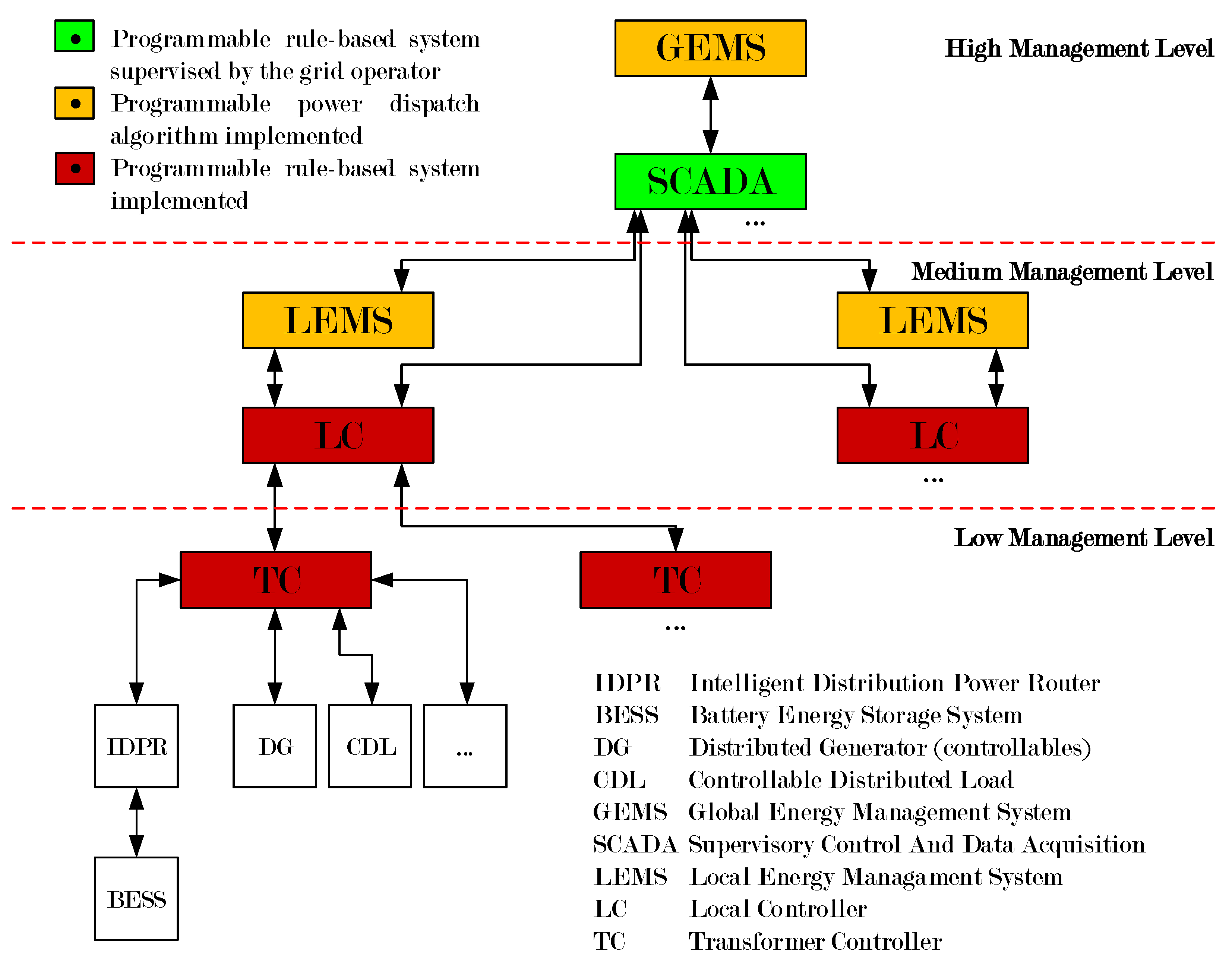
The energy management system is composed by diverse agents, which from a top-down approach are: (i) the Global Energy Management System (GEMS); (ii) the Supervisory Control and Data Acquisition (SCADA); (iii) the Local Energy Management Systems (LEMSs); (iv) the Local Controller (LC); (v) Transformer Controllers (TCs) and finally, at the bottom of the structure there are all manageable and controllable equipment.
All of them configure a system in the form of that presented in Figure 1. As can be observed the different agents of the system are distributed into three management levels. At the top level there are the SCADA and the GEMS. Both agents are the responsible of the proper operation of the whole Distribution Network (DN). At the intermediary layer there are LEMSs and LCs. These two types of agents are in charge of the operation of limited parts of the DN. Finally, at the bottom level there are the TCs that manage and control Secondary Substations’ (SS) equipment. Depending on the relevance of each SS, an area can collect one or more SSs.
The management agents in Figure 1 are also classified in terms of their programmability (see the color code). In this regard, the SCADA is the agent with the highest level of programmability. It is a rule-based system supervised and managed by the DSO.
Just below the SCADA there are the GEMS and the LEMS. In terms of programmability, these agents determine the series of active and reactive power setpoints for optimizing the whole or part of the rural DN. Also, they calculate, on a one minute basis, the setpoints to manageable and controllable equipment, such as some Distributed Generators (DG), Controllable Distributed Loads (CDL), Diesel Generators (GS) and back-up resources (or, as named, Intelligent Distributed Power Routers (IDPRs), with Battery Energy Storage Systems (BESS)).
The IDPR is a power converter that improves the power quality and if it allocates a BESS, then it also manages energy packages. The main challenge of the IDPR in terms of power quality is to compensate for unbalanced currents (of the three-phases), compensating reactive power and cancelling the harmonic content of currents at coupling point, in a slave mode. Also the IDPR can storages energy from distributed generation and provides it during pick hours or during a supply disruption, since the IDPR is the responsible to restore the supply in the network providing a voltage and frequency of the local set, in a master mode [40,41].
Finally, the LCs and TCs are programmable rule-based devices that exchange information and setpoints with the back-up resources, DGs, CDLs, GSs, as well as with control and protection devices. It is important to note that the programmable rule-based systems implemented in LCs and TCs ensure a proper operation during an eventuality in the communications’ network.
This paper focus on the GEMS agent while managing the whole DN. To do so, this agent optimizes the operation of the network in two main steps. The first step—called economic optimization hereinafter, solves an optimal economic dispatch for the controllable sources and loads in the network. Since economic, the optimization is based on market aspects, availability and cost of DGs and back-up resources. The second step, and from the inputs of the first one, adjusts the active and reactive power dispatch for DGs and back-up resources considering technical aspects such as power losses and voltage variations, thus performing an Optimal Power Flow (OPF) [42]. This paper develops these two management steps performed by GEMS under the operational circumstance that the rural grid being managed is not isolated, but connected to the main grid of the rest of the territory.
So more in detail, the GEMS performs the following tasks: (i) generates the consumption and generation forecasts for the whole system and for a time horizon of 24 h; (ii) with this time horizon, executes the global economic optimization; (iii) executes the optimal power flow function of the global economic optimization setpoints and network technical constrains; (iv) outputs a file with the setpoints for controllable sources and loads for the following 24 h, in time steps of 15 min. Such time step is convenient for the integration of GEMS in some electrical markets worldwide [43,44]. The following Section 3 develops the presented objectives for GEMS step-by-step.
3. The Global Energy Management System
This section introduces the GEMS operation. Internally, the GEMS has three different modules addressing its objectives. The first module carries out forecasts. In particular, it determines the generated and consumed forecasts for active and reactive power for each SS. The second module (the Global Economic Optimization (GEO)) processes the price of electricity pool and sends it to SCADA. Also the GEO module calculates through a Mix Integer Lineal Programming (MILP) determines the power setpoints for controllable generators, loads and storages addressing an economic criterion. These setpoints are named global economic setpoints. Finally, these setpoints are processed in the third module of the GEMS, which is called the Global Technical Optimization (GTO) module. The GTO module adjusts through a Non-Lineal Programing (NLP) the global setpoints are according to the technical constraints, applying curtailments if required and adapting the reactive power, in order to smooth voltage variations and reduce the electrical losses. Finally the resulting setpoints, the global technical setpoints are sent to SCADA. The Figure 2 collects the described modules of GEMS and the time horizon for the processes they carry out. The following gives a deeper description of the GEMS.
3.1. Forecasts for the Whole System
Currently, the models to forecast the electrical consumption and generation, are tools that are developed for specific areas. They function in several aspects like, economic, weather, industry, population, market, technological development, among others [9]. In addition, in the literature there are several techniques that related all these inputs to determine the outputs. Commonly they can be classified into static or dynamic, univariate or multivariate and for the technique that they use. The most simple and frequent techniques are times series and regression models [9].
The aim of the article is not to advance in the knowledge field of the forecast methods. So the required forecasted data for GEMS operation has been derived from real data adding a random variability according real standard deviation. The root-mean-square of the error for simulated forecasted data is 10%. This is consistent with usual error magnitude provided by state-of-the art forecasting methods for wind and sun resources [9].
3.2. Global Economic Optimization Formulation
The Global Economic Optimization formulation is a MILP model that pursues DSO’s goals. As noted in Figure 2, the GEO is the first optimization block in the GEMS algorithm. Its objective is to solve with an minimum energy cost for grid participants, and this is translated into a quarter-hourly dispatch for distributed resources. For GEO formulation the following hypotheses are considered:
- It optimizes the dispatch of active power for controllable elements in the network, assuming that the reactive power management is treated by the GTO.
- It assumes that the DN operates as a three-phase balanced system, so power flows among three phases of the DN are aggregated for optimization purposes. Such a balanced system is ensured by the action of the previously introduced IDPRs. The IDPR makes the unbalanced power flow downstream (i.e., in the low voltage network, where dispersed consumers and generators are located) as an aggregated balanced power flow upstream to be exchanged with the medium voltage DN.
- It also assumes that voltage levels remain in an acceptable range, thanks to the subsequent GTO actuation.
- It does not take into account the electrical losses of lines and transformers.
- It takes into account the performance of storage technologies. The efficiency in charging and discharging processes as well as the self-discharge phenomena are considered.
- The number and consumption of controllable loads is known.
- The number and output of programmable generators is known.
- The consumption and generation at SS feeder is aggregated, representing the behaviour of low voltage network.
Following contents present the input data, variables, mathematical constraints and the objective function for the GEO.
3.2.1. The Input Data
3.2.2. Variables
3.2.3. GEO Constraints
In turn constraints are also divided and formulated in four groups, (i) SSs and the EG, (ii) DSMs, (iii) DGs and (iv) BESSs constraints.
(i) SSs and EG constraints
The power balance constraint (1) determine the energy exchanged by each SS. This must be equal to the sum of the energy consumed and generated by customers, and the energy supplied (or consumed) by the storage systems. In addition, this also is bounded by the rated power of the SS transformer in (2). Then, in (3), the sum of all exchanged energy is equal to the difference between the imported and the exported energy from the EG. Finally, imported and exported energy from the EG are limited by the rated power of the EG transformer through (4) and (5), also ensuring that when one is positive the other is zero and vice versa.
(ii) DSM constraints
The energy consumed, as detailed in the (6), is the sum of the energy from non-controllable and controllable distributed loads, as well as the energy not supplied to loads. Typically, CDLs are characterized by their rated power and the time they are consuming energy. These two variables are bounded by Equation (7) (power) and Equation (8) (time). Finally, the Equation (9) restricts the consumption of CDLs for the time interval addressing starting times.
(iii) DG constraints
Equation (10) sums the energy generated by all different DG sources. Equation (11) fixes the generated and the non generated energy from NCDGs according to forecasts. The generated and non generated energy from SDGs are quantified by Equations (12) and (13), respectively. Similarly, generated and non generated energy by ADGs are quantified by Equations (14) and (15). Similarly to CDL Equations (7)–(9), Equations (16)–(19) determine the generated and non generated energy from PDGs in function of their rated power and operating times . Finally, the energy generated by PADGs are determined by Equations (20)–(23). The total generation for each SS is determined by Equation (20), and Equation (21) limits the output power of PADGs according to their limitations. Further, the fuel consumption per each unit is calculated by Equation (22) and limitations in fuel usage are imposed by Equation (23).
(iv) BESS constraints
Completing the description of the constraints for the problem, BESS-related constraints are introduced in the following. Equation (24) defines as the subtraction between the energy consumed and injected to the grid by storages. In turn, these terms are limited by Equations (25) and (26), which are function of the rated power of the battery (). In addition, the State of Charge (SoC) is bounded by Equation (27). The SoC is in function of the capacity of the battery (), the initial SoC (), the self-discharge constant (), and the charging and discharging efficiencies, () and () respectively.
3.2.4. The GEO Objective Function
The global economic objective function has been chosen incorporating diverse criteria. Addressing the obligation for DSOs to cover the demand, the first summation of the objective function calculates the cost for the energy not supplied to DLs (including the non controllable DG). Note that the second to fourth summations are included in order to maximize DGs generation and manage them efficiently. Further, the fifth summation aims to minimize the cost related to fuel usage (including the wasted fuel). Finally, the last summation is added so as to minimize the cost related to energy imported from the EG.
3.3. Global Technical Optimization
As noted in Figure 2, the Global Technical Optimization is the last optimization procedure in the GEMS. It receives the outputs from GEO and perform a process based on a NLP that provides the final setpoints for distributed resources according to the DSO’s technical constraints. The GTO minimizes losses in the DN guaranteeing the dispatch solved by the GEO. The GTO also adjusts the reactive power from the IDPRs, and also readjust the active power from DGs and BESS in order to keep the voltage within acceptable range. The GTO goes under the following assumptions:
- The DN voltages and currents are balanced.
- Consumption and generation profiles are aggregated at each SS’s feeder.
- The electrical loses of medium voltage lines and transformers are considered for optimization purposes.
The following presents the input data, variables, mathematical constraints and the objective function for the GTO.
3.3.1. The Input Data
3.3.2. Variables
3.3.3. GTO Constraints
In turn constraints are also divided and formulated in three groups, (i) voltage and total power, (ii) EG, (iii) SS constraints.
(i) Voltage and total power constraints
(ii) Constraints related to the EG bus
Active and reactive power balances at the EG bus are ensured by Equations (33) and (34), respectively. The active and reactive power balance for the rest of buses are ensured by Equations (35) and (36). Equation (37) establishes that the active and reactive power exchanged with the EG is less than the rated power of the EG transformer. The voltage module and angle of the EG bus is fixed by Equations (38) and (39), respectively.
(iii) Constraints related to SS buses
An excessive voltage level at SS buses is quantified by Equation (40). The active power generated by DGs is bounded by Equation (41). Similarly, the Equation (42) limits the active power injected from BESSs of IDPRs. The active power term can be negative and this means that the battery is consuming power. Therefore, the DG production could be reduced, the BESSs could dispatch or absorb energy. Finally, the active and reactive power supplied by IDPR is bounded by Equation (43) and the total power exchanged by a SS is bounded by the rated power of transformer through Equation (44).
3.3.4. The GTO Objective Function
The technical objective function is divided into terms, the first one minimizes the imported energy from EG, thus indirectly minimizing the electrical losses and maximizing the active power generation from distributed resources. The second penalizes any excess or deficit in voltage for all buses through the weighting factor. This factor penalizes an excess of voltage in terms of active power ().
4. Study Cases
For GEMS performance evaluation, different computational scenarios and metrics are proposed, and these are presented in the following.
4.1. Definition of Computational Scenarios
Twenty computational scenarios are proposed for evaluation. The scenarios are distributed in four blocks:
- Case (i): The DN neither includes IDPRs neither BESSs, nor management tools.
- Case (ii): The DN is equipped with IDPRs and BESSs, and the GEO, as a management tool.
- Case (iii): The DN is equipped with IDPRs and BESSs and the GTO, as a management tool.
- Case (iv): The DN is equipped with IDPRs and BESSs, as well as the GEO and the GTO as management tools.
Doing this, it is possible to evaluate the impact in network operational performance of adopting both the energy management algorithms proposed in this paper as well as the IDPRs, as distributed energy storage capabilities.
For each of the above presented blocks, five scenarios are proposed, each proposing different levels of renewables’ penetration. In particular, DG penetration varies from 10% to 50% with respect to total contracted power in the network.The DG penetration is bounded in Spain up to 50% of total contracted power by current regulation [45].
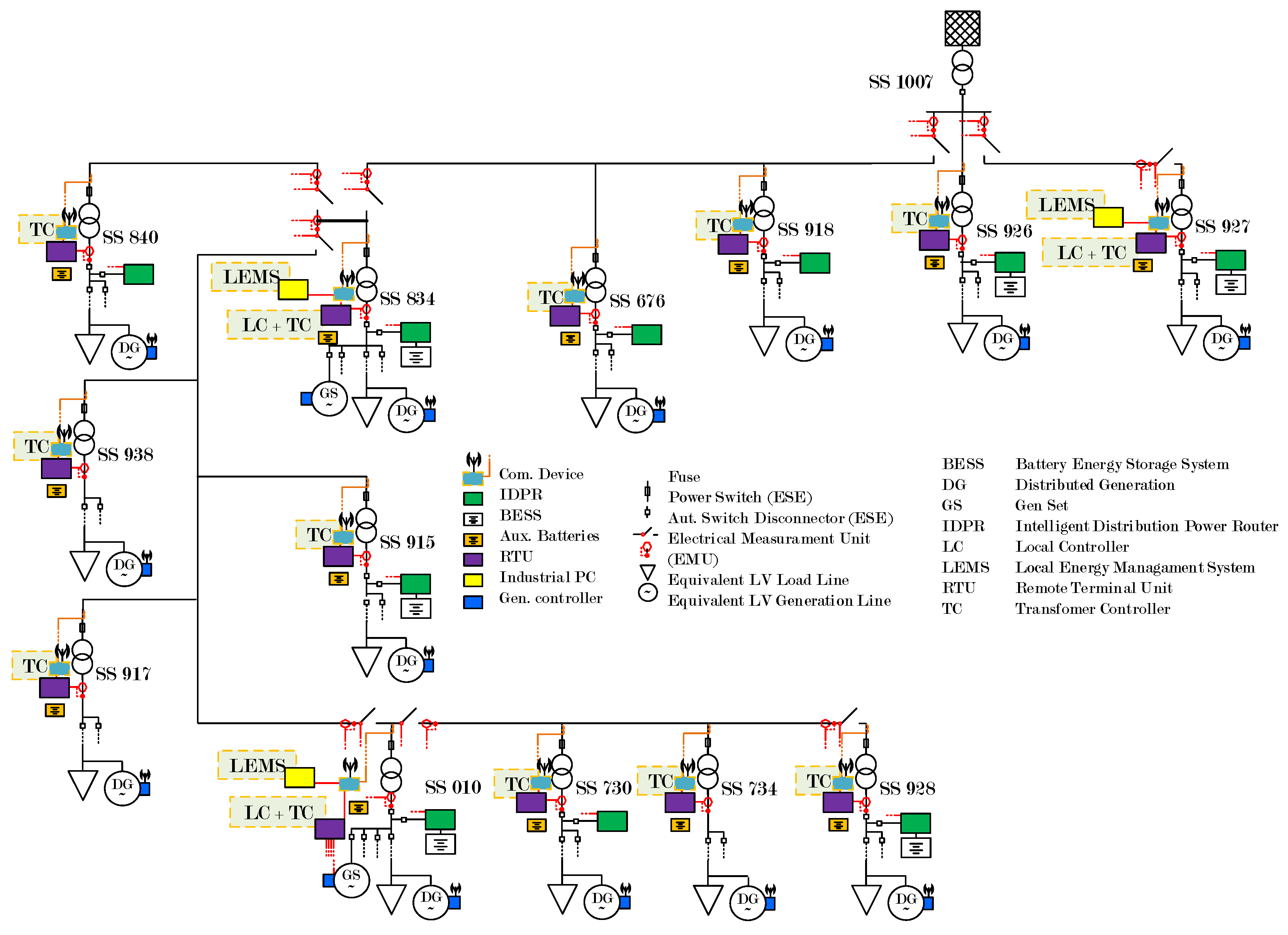
The adopted DN is located in a rural zone of Catalonia [46]. This grid is actually being utilized as a demonstration site for the management tools and power electronics (the IDPR) presented in this paper. These demonstrations are being carried out in the frame of the FP7 European research project Smart Rural Grid. Figure 3 presents a single-phase diagram of this DN.
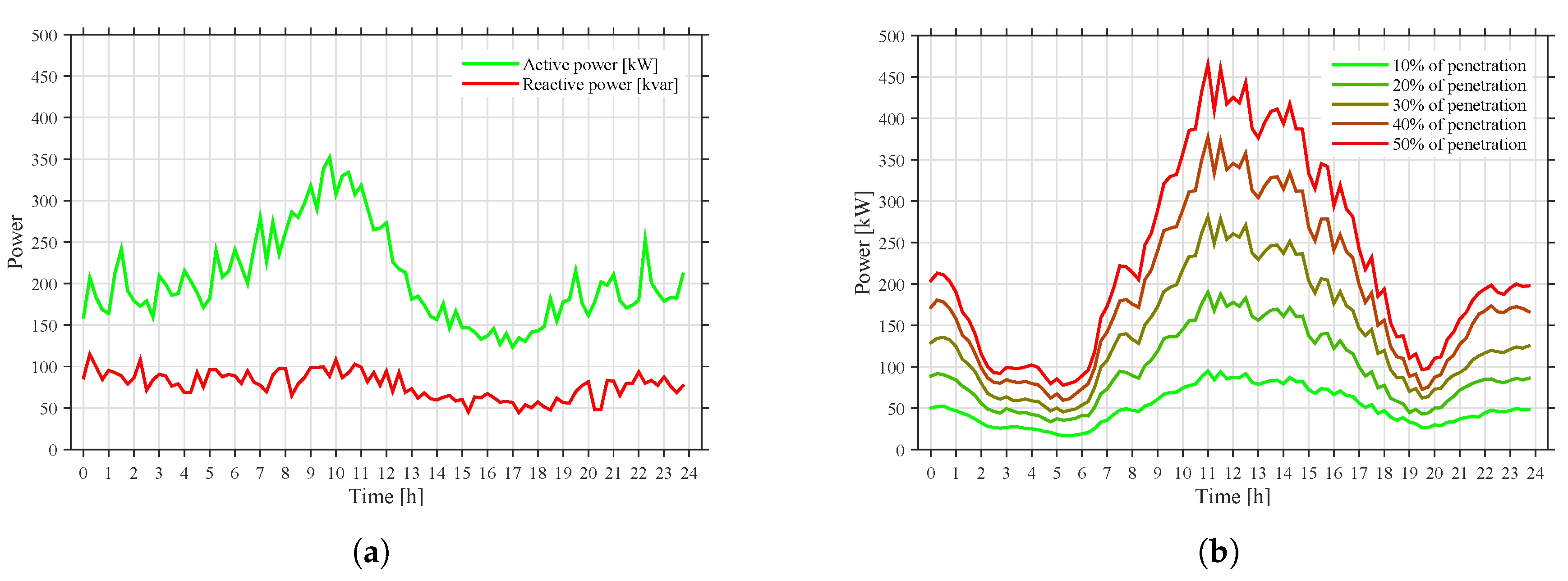
As can be noted, this is a rural distribution grid including 13 SSs. The consumers are of different types, including DLs, NCDLs and CDLs. The CDLs refers to electrical vehicles, water heaters, refrigerators. A penetration of about 25% of CDLs are integrated in each SS. Moreover, several types of DGs are included in the network: (i) non-controllable DGs (small or micro renewable generation like flow-hydraulic generation, photovoltaics and wind-based generation); (ii) switchable and adjustable DGs (renewable sources governed by microcontroller that regulate their power output; (iii) programmable DGs (fully governable generators such as combined heat and power generation systems); and iv) programmable and adjustable DGs (auxiliary sources like diesel, biomass, gasifiers, waste-to-energy generators). A representative daily profile for aggregated generation and consumption are presented in Figure 4.
4.2. Power Quality Indicators and Metrics
This section introduces diverse quality indicators so as to evaluate the impact of including the management tools proposed in this paper. Similarly as for parameters and variables, quality indicators are divided into two groups, (i) secondary substation indicators () (see Table 18), and (ii) distribution network indicators () (see Table 19).
(i) SS related metrics
The indicator expresses through Equation (46) the voltage width of the 95% of SS voltage module of a day (). This metric is formulated as in the EN 50160 standard [47]. Note in Equation (46) that is the nominal value of voltage for this bus. Analogously, the SS indicator is related to the total reactive power over the active power consumption, and the SS indicator determines the average energy discharged by batteries for each SS. Finally, the SS expresses how much power is curtailed from the maximum power available from DGs for each SS.
(ii) DN related metrics
The DN indicator is calculated from the total electrical losses of the whole DN (from passive elements) divided by the total power consumption. Note that the energy losses from passive elements is determined by the Equation (53). The DN indicator presents the percentage of the consumption of IDPRs and BESSs respect to the total power consumption. Note that the energy losses from the active elements is determined by the Equation (55). The DN indicator determines how much power is imported from the EG respect to the total power consumption through Equation (56).
4.3. Simulation Results
This subsection depicts the simulation results for the four blocks of scenarios, which in turn include five levels of DG penetration. As a reminder, each of the four cases are characterized by including different energy management tools and energy storage devices.
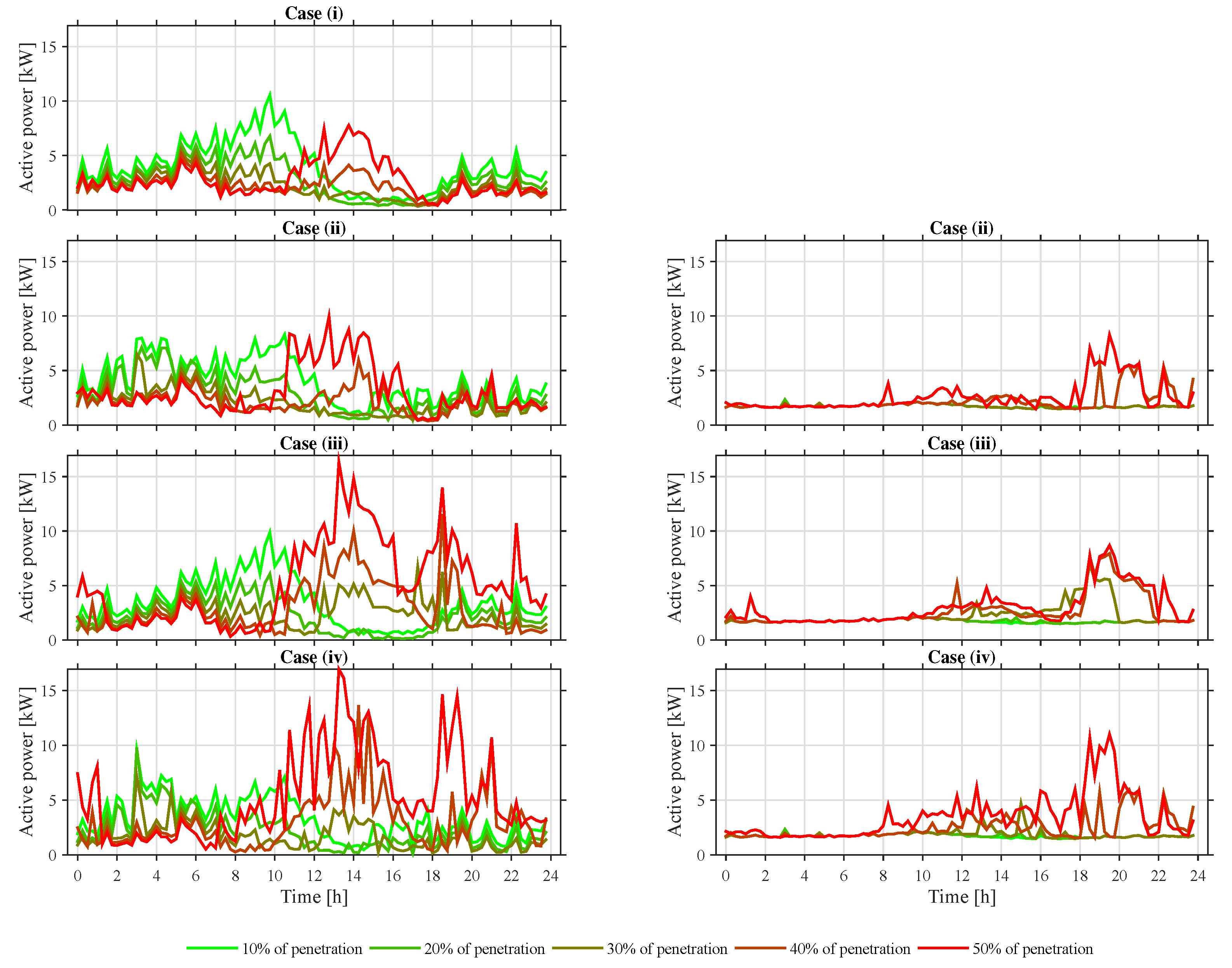
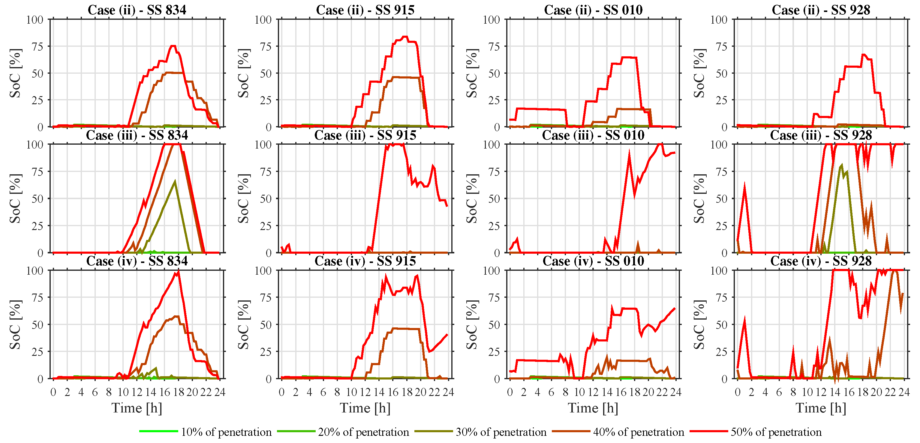
Graphical results are structured in the following Figures (Figure 5, Figure 6, Figure 7 and Figure 8). Figure 5 plots the power exchanged (both active and reactive) with the EG for each of the four cases of scenarios. Analogously, Figure 6 plots the power losses. In addition, Figure 7 presents the the voltage in SS 834, 915, 010 and 928. Figure 8 plots the SoC of BESS at SS 834, 915, 010 and 928.
To sum up, SS and DN indicators, and objective functions (are defined in Section 3.2 and Section 3.3) are calculated and presented in Table 20, Table 21 and Table 22, respectively. Note that there are many SSs, so Table 20 only presents average and peak values from SSs.
Further, it is interesting to note that assessing the impact of forecasting errors for generation and demand in indicators included in the above mentioned tables, additional simulations were performed, in which no forecasting errors were considered. The comparison of the results indicate a little influence in the indicators. For instance, the indicator associated to the usage of batteries () has experienced a variation around 1.97% (so less than 2% on average) from these two simulations. Similarly, the indicator addressing the renewables’ curtailment () has varied about 1% on average. Indicators addressing voltage quality (), power factor () and power losses ( and ) has remained almost equal for the two simulations.
5. Discussion of Results
This section presents a discussion of the optimization results. The optimization is carried out through Julia software [48,49] using the mathematical language called Jump [50] and optimization solvers called Gurobi [51] and Ipopt [52]. Then, the obtained data is thread and depicted through mathematical software (Matlab) [53]. The discussion of results is in terms of the indicators previously defined, which focus on the secondary substations (SS indicators) and of the rest of the elements of the distribution network (DN indicators).
5.1. SS Related Metrics
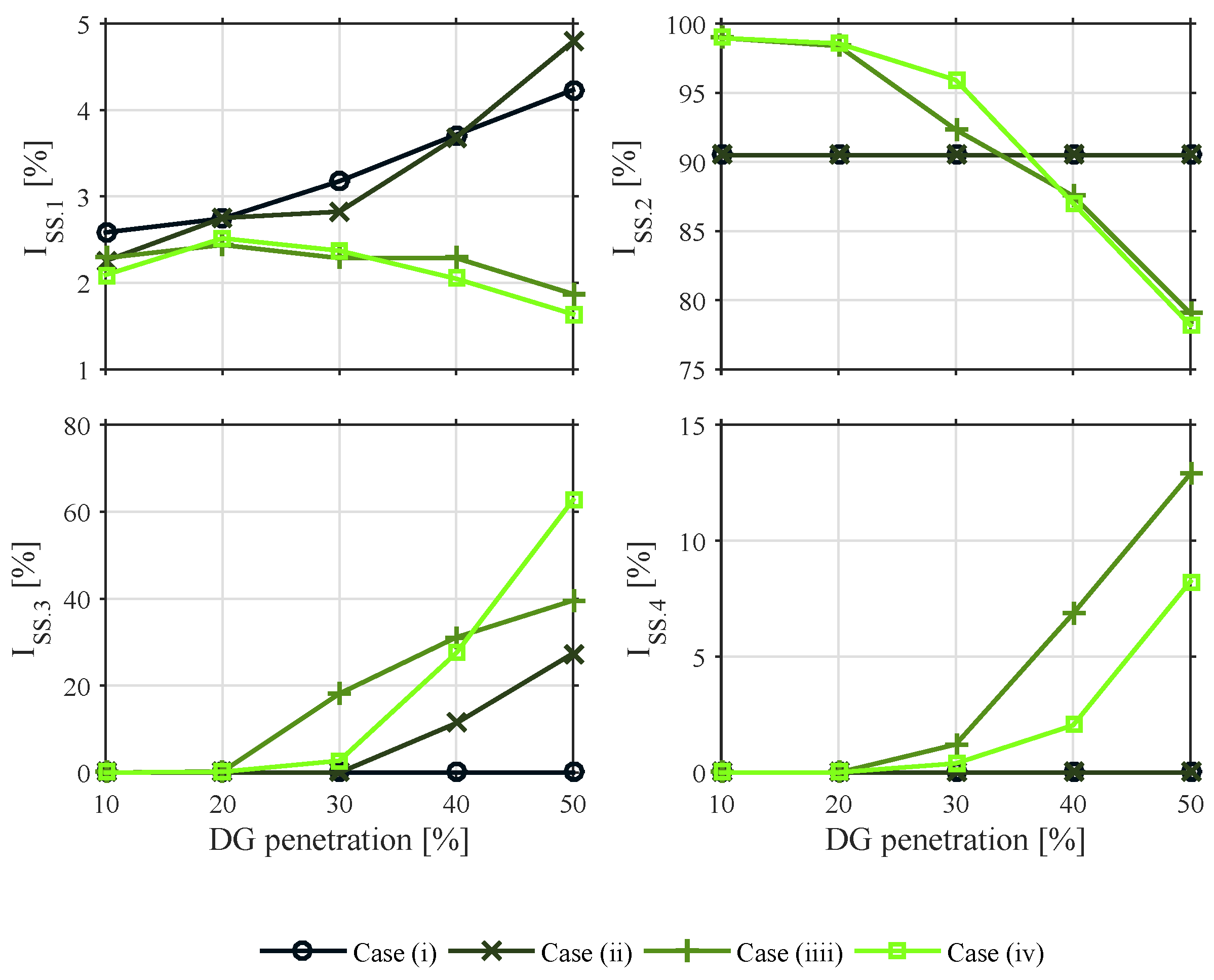
(i) Voltage quality related metric ()
The voltage metric is directly related with Figure 7. This reflects that the quality of the voltage at the SSs tends to decrease with the distance of these SSs to the point of interconnection with the transmission system. It is remarkable to note that this trend is accentuated if the network is operated from just an economic criterion, i.e., through the GEO (see the results for case (ii) in Figure 7). However, if it is applied the technical operation strategies –the GTO– (see cases (iii) and (iv), the metric results clearly improved with respect to base cases (i.e., case (i) with respect to case (iii); and case (ii) with respect to the case (iv)). This can be clearly observed in Figure 9, upper left subplot.
(ii) Reactive power related metric ()
It is considered that the reactive power is only associated to the loads of the network; generators are operated with an unitary power factor. Therefore, this metric does not depend on the DG penetration level for cases where there is not reactive power management –the GTO– (cases (i) and (ii)). However, when there is reactive power management (cases (iii) and (iv)), there is a dependency between DG penetration and the reactive power metric . This can be reflected in Figure 9, upper right subplot. For low levels of DG penetration, the reactive power management focuses on reducing electrical losses. As a reminder, this reactive power management is performed by the IDPRs, not by DG. Conversely, for DG penetration levels above the threshold level of 30%, from which active power flows through the network are highly variable, the reactive power management is under the criterion of smoothing voltage variations. As a consequence, the reactive power metric decreases. This progressive worsening of metric is also appreciated in Figure 9, upper right subplot.
(iii) Battery related metric ()
The battery usage is directly related with the level of DG penetration (see SoC variations for all cases evaluated in Figure 8, clearly showing how batteries are more and more operated with increasing DG penetration levels). For all cases and regardless the usage level of the battery, they are charged with surplus of DG. Still keeping the attention in Figure 8, we can observe two additional aspects. First, for the case in which the network is operated under an economic criterion, i.e., case (ii), the GEO decides to let batteries completely discharged at the end of the day for economic purposes. This way, batteries are charged in sunny hours, with surplus of renewables, and discharged at night, when electricity is costly and there is no surplus of renewables. Second, for the case in which the network is operated also under the technical criterion (i.e., cases (iii) and (iv)), batteries are also operated so as to improve the power quality of the network (for instance to smooth out voltage variations). As a consequence, the usage of the batteries is higher than in the case (ii), specially for DG penetrations above 30%.
(iv) Curtailment related metric ()
The curtailment related metric is directly associated to the level of DG penetration and management tools applied. For low DG penetration levels, the curtailment is not relevant (see Figure 9, bottom right subplot). Conversely, for DG penetration levels above 30%, curtailment is an issue and a matter being dealt by solely the GTO (case (iii)) or both the GTO and the GEO (case (iv)). For the case (iii), and as shown in Figure 9, a noticeable share of DG generation results curtailed with the objective of maintaining a minimum power quality in the network. Note for instance in this regard, that up to 12% of renewables should be curtailed considering a DG penetration level of 50%. For the case (iv), in which the network is operated by both the GTO and the GEO, this latter management algorithm decides to reduce the amount of energy curtailed so as to minimize economic costs of network operation, while still respecting the technical optimization proposed by GTO.
5.2. DN Related Metrics
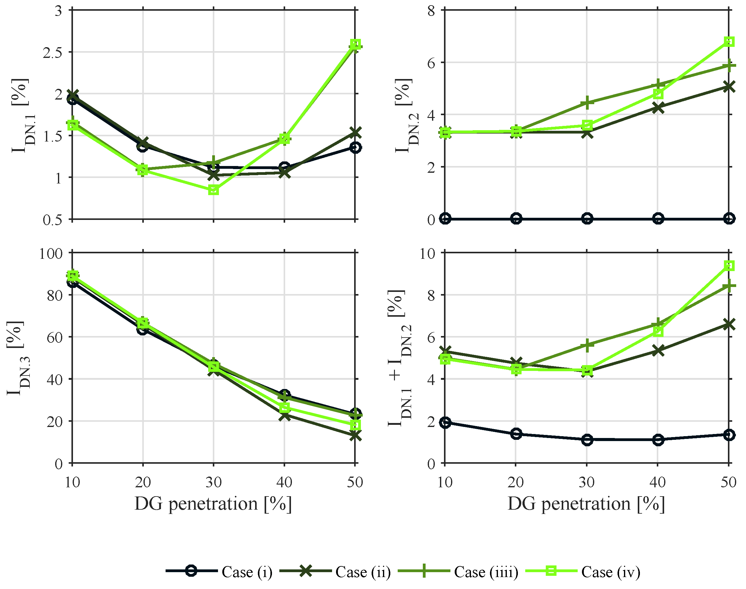
(i) Distribution electrical losses (cables and transformers) ()
Passive losses are proportional to the square of current. As can be observed in Figure 6, they are significant during peaks of demand and/or generation. Also in the above mentioned figure, for the case (i), when the DG penetration level is low the major part of electrical losses are during peak demand hours (i.e., in the morning). Conversely, while the DG penetration level is high, the major part of electrical losses are gathered during the midday (as a result of PV generation).
More in detail, Figure 10, upper left subplot, presents the evolution of metric (so the magnitude of distribution losses) function of DG penetration levels. As can be observed, for low shares (below 30%) and considering the application of the advanced management tool GTO (case (iii) and case (iv)), passive losses become lower than for the base case (case (i)). However, for penetration levels above the threshold of 30%, the actuation of the GTO, which is focused on smoothing voltage variations, affects distribution losses increasing them above the base case. It is important to highlight that active losses remain almost constant during the day. However, in the evening, they experience an increment as a result of the process of batteries discharging. Finally, in case (i) there are not active elements involved, such as IDPRs and BESSs, so there are not associated electrical losses to compute.
(ii) Electrical consumption of IDPRs (active elements) ()
This electrical consumption is additional to the base case. This is a toll that smart grids have to pay in order to include additional equipment as power electronics and batteries. However, it represents a small percentage of all consumptions, similar to cables and transformers. As can be observed in Figure 10, in general terms, the higher the DG penetration is, the more we utilize batteries and power electronics, and thus the higher the associated losses are. Finally, note that this usage of batteries is mainly bounded at night, since is in this time frame in which batteries are discharged (see Figure 6).
(iii) External dependency ()
It is noted that the dependency with the EG is inversely proportional to DG penetration level. Such dependency with the EG is even lower if the network is managed by the GEO (please compare cases (i) and (ii) in Figure 10 bottom left subplot). From this comparison, it can be observed that is improved up to 10% approximately at most while considering the GEO. This can also be observed in Table 21. Even though this improvement could seem relatively small, the impact of including the GEO as the management tool results much more important in economic terms, as analysed later in Section 5.3. In addition, an important aspect to highlight at this point is the effect of CDLs and PDGs in external grid dependency. The management of such resources permit time shift consumption and generation according to electricity prices. In other words, CDLs consume when there is an energy surplus or when the energy is cheap, and PDGs generate when there is an energy deficit or when it is expensive. The effect on this management is reflected in Figure 9, comparing cases (i) and case (iii) (cases with no management of CDLs and PDGs), with cases (ii) and (iv), in which there is management for such controllable resources. It can be observed how demand peaks are moved to off-peak periods (for instance, see the load peak reduction in the morning for cases with renewables penetration of 10% and 20%).
5.3. Evaluation of Objective Functions
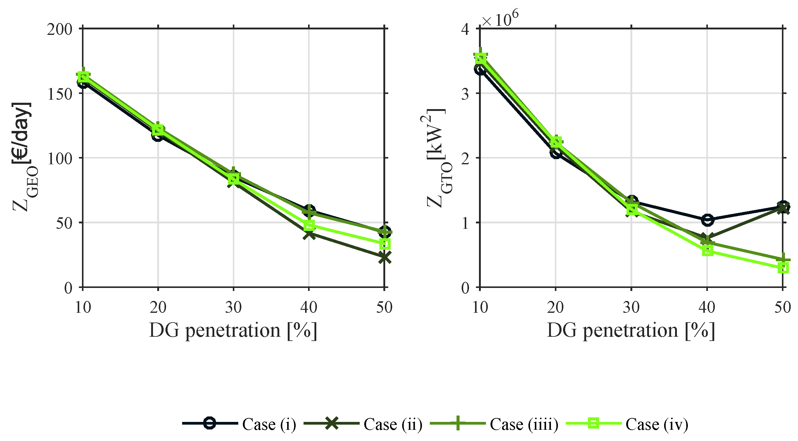
(i) The GEO objective function ()
As a reminder, the GEO tries to minimize the operational costs of the DN. As can be appreciated in Figure 11, left subplot, the costs, i.e., , decreases as proportional to DG penetration levels for all cases. This makes sense, since less power is imported from the EG. Such trend is even accentuated for cases (ii) and (iv), where the economic management is applied. In addition, it is worth noting that for low DG penetration levels, the cost is slightly higher than for considering high shares due to the toll associated to the losses incurred in batteries and power electronics. It is important to remark that from 30% of DG penetration on, this additional losses are compensated via the savings from the economic management performed by the GEO. Finally, the cost reduction from cases (ii) and (iv) with respect to the case base (case (i)), is almost 45% and 21%, respectively.
(ii) The GTO objective function ()
As a reminder, the term is related to the magnitude of the power flows between the DN and the EG, and also to the severity of voltage variations within the DN from the desired values. So from a technical perspective, should be as low as possible, indicating somehow minimum power losses and voltage deviations. As depicted in Figure 11, right subplot, in general terms decreases with the DG penetration level. This clearly depicts the progressively dependency reduction with the EG. For the base case though, and also for the case (ii), in which the GTO are not working, there is point, around 40% in DG penetration, that voltage variations are remarkably high, and this makes to increase. On the other hand, for these scenarios in which the penetration of DG is above 40%, the operation of the GTO keeps such voltage deviations low, thus ensuring a minimum .
6. Conclusions
This paper addressed the impact of including different advanced techniques for managing electrical rural grids. These techniques combine the application of ICT tools and power electronics with embedded energy storage capability. The analysis was based on a real grid, in which different scenarios have been evaluated and these are characterized by progressively increasing the penetration of renewable energy generation from a base, current case. In these analyses, the temporal profiles for the demand have been also derived from the current ones, and adopted with a 15 min time step resolution.
The new advanced management techniques included: (i) an algorithm named as GEO, able to dispatch the charge and discharge of the energy storage devices throughout the grid, as well as the controllable loads and programmable energy generation capabilities, all of these from an economic criterion; (ii) an algorithm named as GTO, able to dispatch the charge and discharge the energy storage devices, the programmable energy generation capabilities as well, and all addressing active power flows, as for the GEO, but also the reactive power flows throughout the distribution grid. In this sense, the GTO performs the operation of the network in terms of a technical criterion; and (iii) a new power electronics-based device with embedded energy storage capacity named here as IDPR. This device effectively executes the charge and discharge of the storage capabilities throughout the grid (i.e., batteries), and also performs a proper management of reactive power flows according to GTO setpoints.
The obtained results, in general terms, demonstrate that for the adopted grid as the case study, the inclusion of these advanced management techniques from both a technical point of view (i.e., an improvement of the power quality of the network) and an economic perspective (i.e., a reduction of the costs incurred in importing energy from the exterior of the distribution network), is justified with a penetration of renewables higher than the threshold level of 30%. From this level of penetration on, the reduction of the costs due to the energy imported with the external grid compensates the toll to be paid in the form of the additional losses of the new energy storage devices integrated into the grid. To emphasize, such thereshold level in penetration of renewables is particular for the adopted study case and cannot be generalized. However, the performed management tools and related metrics could be directly applied for analyzing other networks.
Also from this level of penetration on, the inclusion of these new management tools (ICTs and energy storages) does improve the techno-economic operation of the grid. This means that the voltage profiles throughout the network result much more consistent and smoothed, and that the dependency with the external network is much lower than in the case of not considering such management tools. For instance, the included energy storage systems, properly managed by the GTO and the GEO, permit to reduce the operation costs, which are mainly affected by the energy imported from the external grid, from 42.5 €/day (case (i), or base case) to 23.4 €/day (case (ii), GEO working), for the case of 50% of renewables’ penetration. Further even, the operating costs of the network as calculated by the sum of the cost of the energy imported from the external grid, the distribution losses and the investments in power electronics as well, result lower while managed by the GEO than in the base case.
More in particular, the inclusion of just the GTO algorithm (not in combination with the GEO) cannot be justified in economic terms. In the same manner, the inclusion of the GEO can be justified from an economic perspective, but not from a technical point of view. The combined actuation of both algorithms yields satisfactory results from both perspectives.
The inclusion of such management tools from a technical perspective can be justified for weak and radial networks concerning long distances, which is the typical case for rural networks. These networks experiences high variations in voltage levels and these become accentuated with the distance from the point of interconnection with the main external grid. These problems are further accentuated with the inclusion of renewables, since voltage variations can be noticeable especially at the end of lines.
Finally, it is worth noting that the analysis proposed in this paper is representative of a case with growing importance of renewables in rural distribution grids. So it is, without any doubt, a timely exercise and in response to the urgent energy transition the electrical power sectors are currently undergoing.
Acknowledgments
The research leading to these results has received funding from the European Union seventh framework programme FP7-ICT-2013-11 under grant agreement 619610 (Smart Rural Grid). This work has also been funded by the programm PDJ 2014, under the grant agreement 2014 PDJ 00091 by the Agència de Gestió d’Ajuts Universitaris i de Recerca.
Author Contributions
Francesc Girbau-Llistuella and Andreas Sumper conceived the scope of the paper; Francesc Girbau-Llistuella conceived and performed the simulation analyses, Francesc Girbau-Llistuella and Francisco Díaz-González analyzed the results; Francesc Girbau-Llistuella and Francisco Díaz-Gonzalez wrote the paper; and Andreas Sumper performed revisions before submission.
Conflicts of Interest
The authors declare no conflict of interest.
Abbreviations
The following abbreviations are used in this manuscript:
| ADG | Adjustable Distributed Generator |
| BESS/BS | Battery Energy Storage System |
| CDL | Controllable Distributed Load |
| DER | Distributed Energy Resources |
| DG | Distributed Generator |
| DL | Distributed Load |
| DN | Distribution Network |
| DSM | Demand-Side Management |
| DSO | Distribution System Operators |
| EG | External Grid |
| EMS | Energy Management System |
| GEMS | Global Energy Management System |
| GEO | Global Economic Optimization |
| GS | Diesel Generator |
| GTO | Global Technical Optimization |
| ICT | Infomation and Communation Technologies |
| IDPR | Intelligent Distribution Power Router |
| LC | Local Controller |
| LEMS | Local Energy Management System |
| MAS | Multi-Agents Systems |
| MILP | Mix Integer Lineal Programming |
| NCDG | Non-Controllable Distributed Generator |
| NCDL | Non-Controllable Distributed Load |
| NLP | Non-Lineal Programing |
| OPF | Optimal Power Flow |
| PADG | Programmable and Adjustable Distributed Generator |
| PDG | Programmable Distributed Generator |
| SCADA | Supervisory Control and Data Acquisition |
| SDG | Switchable Distributed Generator. |
| SG | Smart Grid |
| SoC | State of Charge |
| SS | Secondary Substation |
| TC | Transformer Controller |
| TSO | Transmission System Operator |
References
- Gómez-Expósito, A.; Conejo, A.J.; Cañizares, C. Electric Energy Systems: Analysis and Operation; CRC Press: Boca Raton, FL, USA, 2008. [Google Scholar]
- Saitoh, H.; Toyoda, J. A new electric power network for effective transportation of small power of dispersed generation plants. Electr. Eng. Jpn. 1996, 117, 19–29. [Google Scholar] [CrossRef]
- Rumley, S.; Kägi, E.; Rudnick, H.; Germond, A. Multi-agent Approach to Electrical Distribution Networks Control. In Proceedings of the 2008 32nd Annual IEEE International Computer Software and Applications Conference, Turku, Finland, 28 July–1 August 2008; pp. 575–580. [Google Scholar]
- Palensky, P.; Dietrich, D. Demand Side Management: Demand Response, Intelligent Energy Systems, and Smart Loads. IEEE Trans. Ind. Inform. 2011, 7, 381–388. [Google Scholar] [CrossRef]
- Strbac, G. Demand side management: Benefits and challenges. Energy Policy 2008, 36, 4419–4426. [Google Scholar] [CrossRef]
- Fang, X.; Misra, S.; Xue, G.; Yang, D. Smart Grid—The New and Improved Power Grid: A Survey. IEEE Commun. Surv. Tutor. 2012, 14, 944–980. [Google Scholar] [CrossRef]
- Gellings, C. The concept of demand-side management for electric utilities. Proc. IEEE 1985, 73, 1468–1470. [Google Scholar] [CrossRef]
- Markovic, D.S.; Zivkovic, D.; Branovic, I.; Popovic, R.; Cvetkovic, D. Smart power grid and cloud computing. Renew. Sustain. Energy Rev. 2013, 24, 566–577. [Google Scholar] [CrossRef]
- Suganthi, L.; Samuel, A.A. Energy models for demand forecasting—A review. Renew. Sustain. Energy Rev. 2012, 16, 1223–1240. [Google Scholar] [CrossRef]
- Zhang, B.; Lam, A.; Domínguez-García, A.; Tse, D. An Optimal and Distributed Method for Voltage Regulation in Power Distribution Systems. IEEE Trans. Power Syst. 2015, 30, 1714–1726. [Google Scholar] [CrossRef]
- Chen, C.; Duan, S.; Cai, T.; Liu, B.; Hu, G. Smart energy management system for optimal microgrid economic operation. IET Renew. Power Gener. 2011, 5, 258. [Google Scholar] [CrossRef]
- Roche, R.; Blunier, B.; Miraoui, A.; Hilaire, V.; Koukam, A. Multi-agent systems for grid energy management: A short review. In Proceedings of the IECON 2010—36th Annual Conference on IEEE Industrial Electronics Society, Singapore, 7–10 November 2010; pp. 3341–3346. [Google Scholar]
- Jebaraj, S.; Iniyan, S. A review of energy models. Renew. Sustain. Energy Rev. 2006, 10, 281–311. [Google Scholar] [CrossRef]
- Kantamneni, A.; Brown, L.E.; Parker, G.; Weaver, W.W. Survey of multi-agent systems for microgrid control. Eng. Appl. Artif. Intell. 2015, 45, 192–203. [Google Scholar] [CrossRef]
- McArthur, S.D.J.; Davidson, E.M.; Catterson, V.M.; Dimeas, A.L.; Hatziargyriou, N.D.; Ponci, F.; Funabashi, T. Multi-Agent Systems for Power Engineering Applications—Part I: Concepts, Approaches, and Technical Challenges. IEEE Trans. Power Syst. 2007, 22, 1743–1752. [Google Scholar] [CrossRef] [Green Version]
- Lu, D.; Francois, B. Strategic framework of an energy management of a microgrid with a photovoltaic-based active generator. In Proceedings of the 2009 8th International Symposium on Advanced Electromechanical Motion Systems & Electric Drives Joint Symposium, Lille, France, 1–3 July 2009; pp. 1–6. [Google Scholar]
- Kanchev, H.; Lu, D.; Colas, F.; Lazarov, V.; Francois, B. Energy Management and Operational Planning of a Microgrid with a PV-Based Active Generator for Smart Grid Applications. IEEE Trans. Ind. Electron. 2011, 58, 4583–4592. [Google Scholar] [CrossRef] [Green Version]
- Zhang, B.; Zhao, C.; Wu, W. A Multi-Agent based distributed computing platform for new generation of EMS. In Proceedings of the IEEE/PES Power Systems Conference and Exposition (PSCE), Seattle, WA, USA, 15–18 March 2009; pp. 1–7. [Google Scholar]
- Tsikalakis, A.G.; Hatziargyriou, N.D. Centralized control for optimizing microgrids operation. In Proceedings of the 2011 IEEE Power & Energy Society General Meeting, 24–29 July 2011; pp. 1–8. [Google Scholar]
- Pedrasa, M.A.A.; Spooner, T.D.; MacGill, I.F. Coordinated Scheduling of Residential Distributed Energy Resources to Optimize Smart Home Energy Services. IEEE Trans. Smart Grid 2010, 1, 134–143. [Google Scholar] [CrossRef]
- Dagdougui, H.; Minciardi, R.; Ouammi, A.; Robba, M.; Sacile, R. Modeling and optimization of a hybrid system for the energy supply of a “Green” building. Energy Convers. Manag. 2012, 64, 351–363. [Google Scholar] [CrossRef]
- Vahedi, H.; Noroozian, R.; Hosseini, S.H. Optimal management of MicroGrid using differential evolution approach. In Proceedings of the 2010 7th International Conference on the European Energy Market (EEM), Madrid, Spain, 23–25 June 2010; pp. 1–6. [Google Scholar]
- Paiva, J.; Carvalho, A. Controllable hybrid power system based on renewable energy sources for modern electrical grids. Renew. Energy 2013, 53, 271–279. [Google Scholar] [CrossRef]
- Alvarez, E.; Lopez, A.C.; Gomez-Aleixandre, J.; de Abajo, N. On-line minimization of running costs, greenhouse gas emissions and the impact of distributed generation using microgrids on the electrical system. In Proceedings of the 2009 IEEE PES/IAS Conference on Sustainable Alternative Energy (SAE), Valencia, Spain, 28–30 September 2009; pp. 1–10. [Google Scholar]
- Conti, S.; Nicolosi, R.; Rizzo, S.A.; Zeineldin, H.H. Optimal Dispatching of Distributed Generators and Storage Systems for MV Islanded Microgrids. IEEE Trans. Power Deliv. 2012, 27, 1243–1251. [Google Scholar] [CrossRef]
- Olivares, D.E.; Canizares, C.A.; Kazerani, M. A Centralized Energy Management System for Isolated Microgrids. IEEE Trans. Smart Grid 2014, 5, 1864–1875. [Google Scholar] [CrossRef]
- Riffonneau, Y.; Bacha, S.; Barruel, F.; Ploix, S. Optimal Power Flow Management for Grid Connected PV Systems with Batteries. IEEE Trans. Sustain. Energy 2011, 2, 309–320. [Google Scholar] [CrossRef]
- Levron, Y.; Guerrero, J.M.; Beck, Y. Optimal Power Flow in Microgrids with Energy Storage. IEEE Trans. Power Syst. 2013, 28, 3226–3234. [Google Scholar] [CrossRef]
- Nikolova, S.; Causevski, A.; Al-Salaymeh, A. Optimal operation of conventional power plants in power system with integrated renewable energy sources. Energy Convers. Manag. 2013, 65, 697–703. [Google Scholar] [CrossRef]
- Lund, H. Renewable energy strategies for sustainable development. Energy 2007, 32, 912–919. [Google Scholar] [CrossRef]
- Karavas, C.S.; Kyriakarakos, G.; Arvanitis, K.G.; Papadakis, G. A multi-agent decentralized energy management system based on distributed intelligence for the design and control of autonomous polygeneration microgrids. Energy Convers. Manag. 2015, 103, 166–179. [Google Scholar] [CrossRef]
- Basir Khan, M.R.; Jidin, R.; Pasupuleti, J. Multi-agent based distributed control architecture for microgrid energy management and optimization. Energy Convers. Manag. 2016, 112, 288–307. [Google Scholar] [CrossRef]
- Dou, C.X.; Liu, B. Multi-Agent Based Hierarchical Hybrid Control for Smart Microgrid. IEEE Trans. Smart Grid 2013, 4, 771–778. [Google Scholar] [CrossRef]
- Zhang, X.; Sharma, R.; He, Y. Optimal energy management of a rural microgrid system using multi-objective optimization. In Proceedings of the 2012 IEEE PES Innovative Smart Grid Technologies (ISGT), Washington, DC, USA, 16–20 January 2012; pp. 1–8. [Google Scholar]
- Arghandeh, R.; Woyak, J.; Onen, A.; Jung, J.; Broadwater, R.P. Economic optimal operation of Community Energy Storage systems in competitive energy markets. Appl. Energy 2014, 135, 71–80. [Google Scholar] [CrossRef]
- Celli, G.; Pilo, F.; Pisano, G.; Soma, G.G. Optimal participation of a microgrid to the energy market with an intelligent EMS. In Proceedings of the 2005 7th International Power Engineering Conference, Singapore, 29 November–2 December 2005; Volume 2, pp. 663–668. [Google Scholar]
- Sugihara, H.; Yokoyama, K.; Saeki, O.; Tsuji, K.; Funaki, T. Economic and Efficient Voltage Management Using Customer-Owned Energy Storage Systems in a Distribution Network with High Penetration of Photovoltaic Systems. IEEE Trans. Power Syst. 2013, 28, 102–111. [Google Scholar] [CrossRef]
- Hatziargyriou, N.; Contaxis, G.; Matos, M.; Lopes, J.; Kariniotakis, G.; Mayer, D.; Halliday, J.; Dutton, G.; Dokopoulos, P.; Bakirtzis, A.; et al. Energy management and control of island power systems with increased penetration from renewable sources. In Proceedings of the Power Engineering Society Winter Meeting, New York, NY, USA, 27–31 January 2002; Volume 1, pp. 335–339. [Google Scholar]
- Shi, W.; Li, N.; Chu, C.C.; Gadh, R. Real-Time Energy Management in Microgrids. IEEE Trans. Smart Grid 2017, 8, 228–238. [Google Scholar] [CrossRef]
- Heredero-Peris, D.; Chillon-Anton, C.; Pages-Gimenez, M.; Gross, G.; Montesinos-Miracle, D. Implementation of grid-connected to/from off-grid transference for micro-grid inverters. In Proceedings of the IECON 2013—39th Annual Conference of the IEEE Industrial Electronics Society, Vienna, Austria, 10–13 November 2013; pp. 840–845. [Google Scholar]
- Heredero-Peris, D.; Montesinos-Miracle, D.; Pagès-Giménez, M. Inverter design for four-wire microgrids. In Proceedings of the 2015 17th European Conference on Power Electronics and Applications (EPE’15 ECCE-Europe), Geneva, Switzerland, 8–10 September 2015; pp. 1–10. [Google Scholar]
- Girbau-Llistuella, F.; Rodriguez-Bernuz, J.; Prieto-Araujo, E.; Sumper, A. Experimental Validation of a Single Phase Intelligent Power Router. In Proceedings of the 2014 IEEE PES Innovative Smart Grid Technologies Conference Europe (ISGT-Europe), Istanbul, Turkey, 12–15 October 2014; pp. 1–6. [Google Scholar]
- Electric Reliability Council of Texas. Real-Time Market. Available online: http://www.ercot.com/mktinfo/rtm (accessed on 14 September 2017).
- Dynamic Pricing in Electricity Supply. Available online: http://www.eurelectric.org/media/309103/dynamic_pricing_in_electricity_supply-2017-2520-0003-01-e.pdf (accessed on 14 September 2017).
- Ministerio de Ciencia y Tecnologia. Available online: https://www.boe.es/boe/dias/2002/09/18/pdfs/A33084-33086.pdf (accessed on 12 December 2016).
- Project Deliverables. Smart Rural Grid Project. Available online: http://smartruralgrid.eu/archive_category/project-deliverables/ (accessed on 1 February 2017).
- AENOR. Norma UNE-EN 50160:2011. Available online: http://www.aenor.es/aenor/normas/normas/fichanorma.asp?tipo=N&codigo=N0046945#.WSwy-mjyjcs (accessed on 29 May 2017).
- Bezanson, J.; Edelman, A.; Karpinski, S.; Shah, V.B. Julia: A fresh approach to numerical computing. SIAM Rev. 2017, 59, 65–98. [Google Scholar] [CrossRef]
- High-Performance Dynamic Programing Language for Numerical Computing. Available online: https://julialang.org/ (accessed on 10 April 2017).
- Dunning, I.; Huchette, J.; Lubin, M. JuMP: A modeling language for mathematical optimization. SIAM Rev. 2017, 59, 295–320. [Google Scholar] [CrossRef]
- Gurobi Optimizer Reference Manual. Available online: http://www.gurobi.com (accessed on 10 April 2017).
- Wächter, A.; Biegler, L.T. On the implementation of an interior-point filter line-search algorithm for large-scale nonlinear programming. Math. Program. 2005, 106, 25–57. [Google Scholar] [CrossRef]
- The MathWorks—MATLAB. Available online: https://mathworks.com/products/matlab.html (accessed on 10 April 2017).
Figure 1.
The multi-agent management system for the smart rural grid.

Figure 2.
Global Energy Management System (GEMS) in detail.
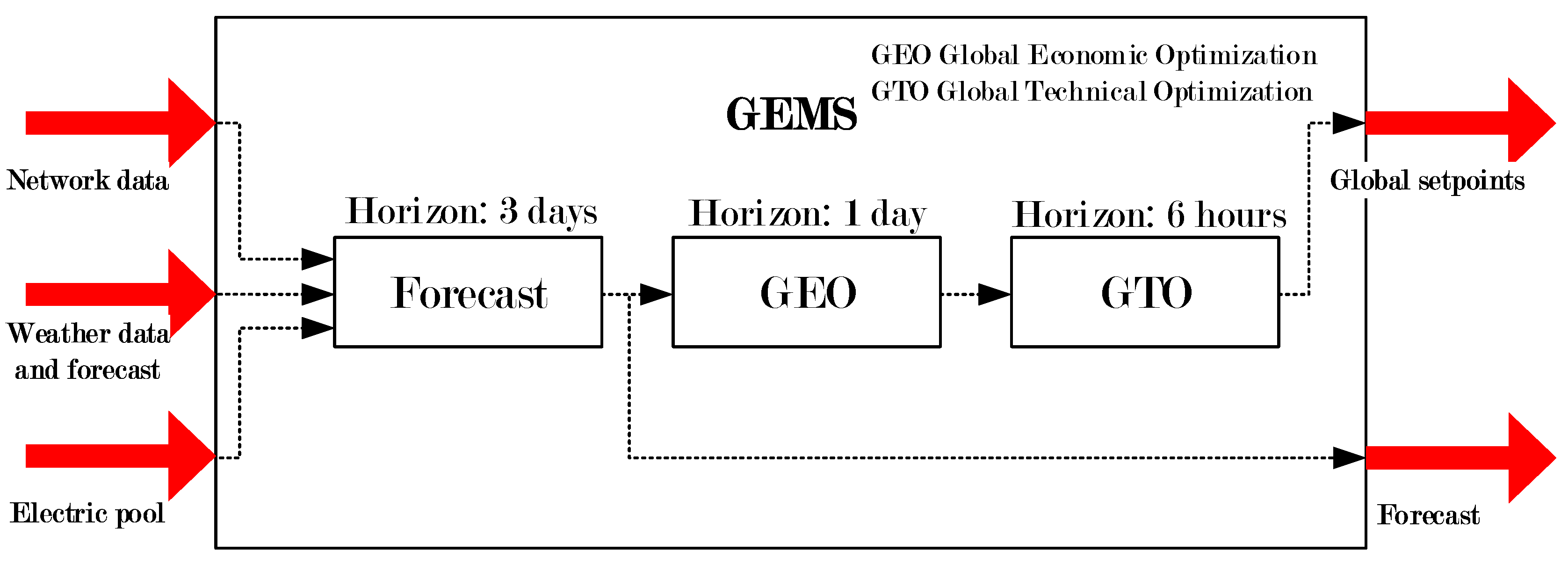
Figure 3.
The whole rural distribution grid.

Figure 4.
Input data. (a): Total active and reactive power consumption of the whole DN. (b): Total active power generated by DGs of the whole DN per different renewables’ penetration.
Figure 4.
Input data. (a): Total active and reactive power consumption of the whole DN. (b): Total active power generated by DGs of the whole DN per different renewables’ penetration.

Figure 5.
Active and reactive power exchanged with the EG (first and second column, respectively) for each block (rows) and for all penetrations (colour scale, legend depicted in Figure 4).
Figure 5.
Active and reactive power exchanged with the EG (first and second column, respectively) for each block (rows) and for all penetrations (colour scale, legend depicted in Figure 4).
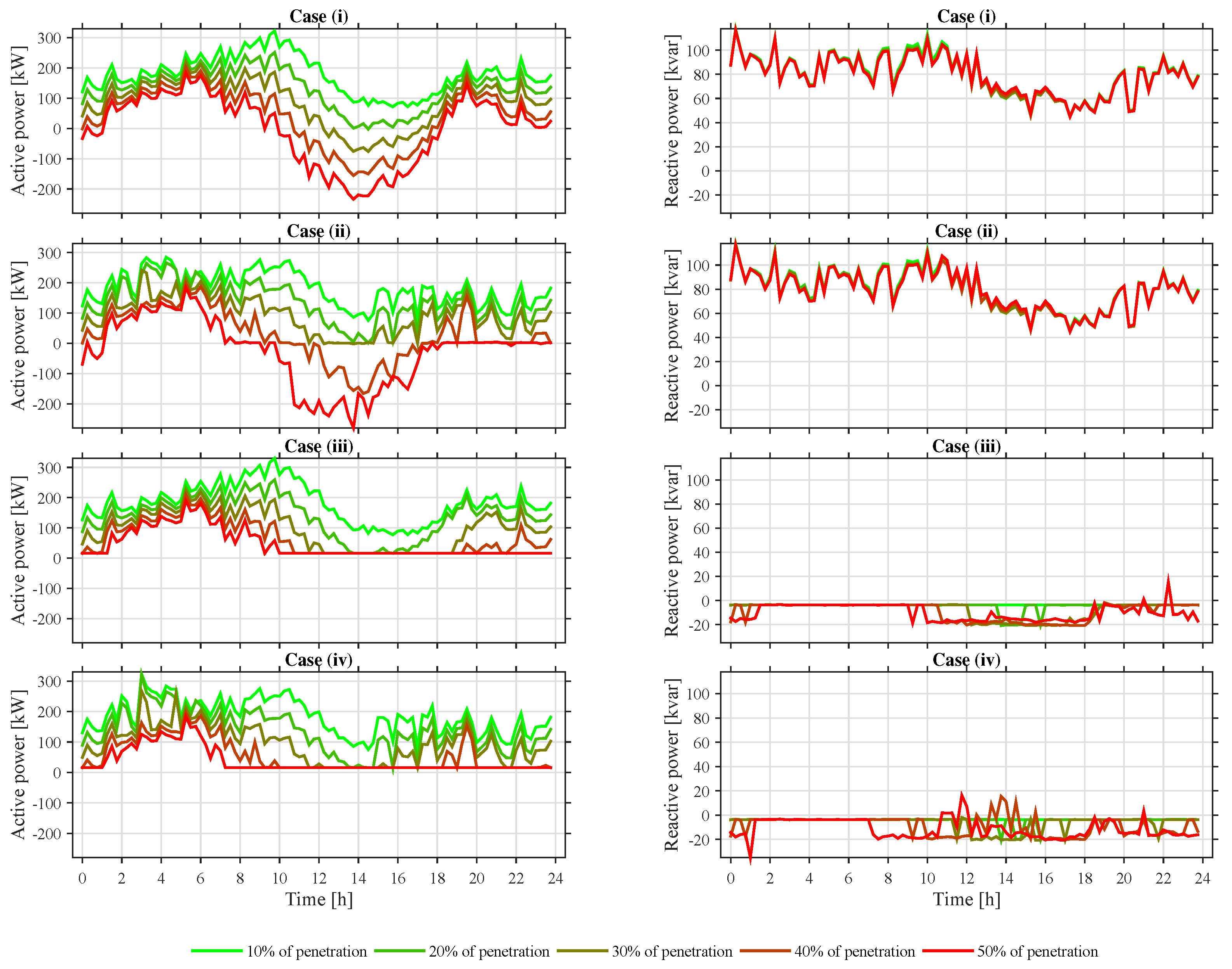
Figure 6.
In the first column: Power losses of DN passive elements for each case. In the second column: Power losses of DN active elements for each case.
Figure 6.
In the first column: Power losses of DN passive elements for each case. In the second column: Power losses of DN active elements for each case.

Figure 7.
Voltage at SS 834, SS 915, SS 010 , SS 928 for each case (rows) and for all DG penetrations (colour scale).
Figure 7.
Voltage at SS 834, SS 915, SS 010 , SS 928 for each case (rows) and for all DG penetrations (colour scale).
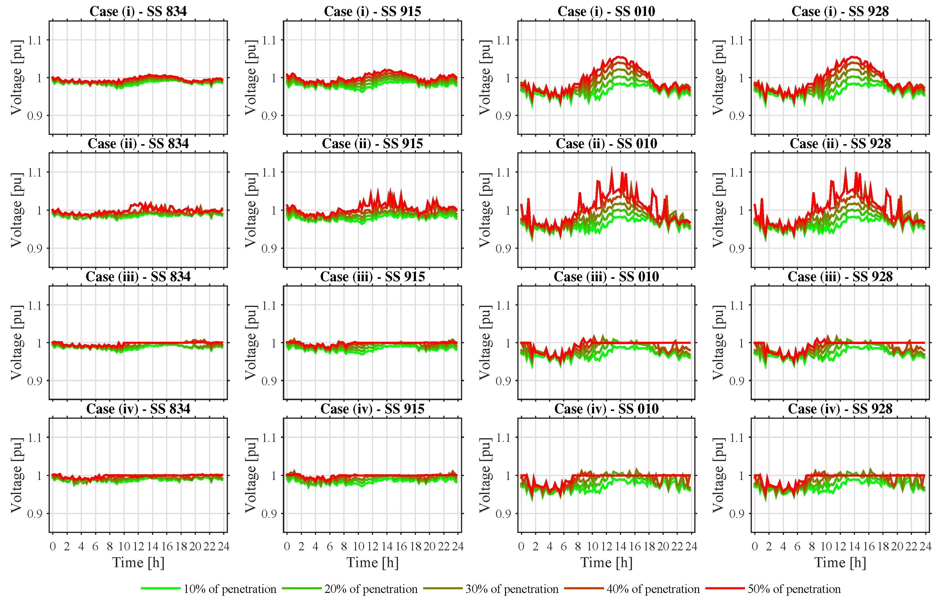
Figure 8.
SoC of BESSs at SS 834, SS 915, SS 010 , SS 928 for cases (ii) to (iv) (rows) and for all DG penetrations (colour scale).
Figure 8.
SoC of BESSs at SS 834, SS 915, SS 010 , SS 928 for cases (ii) to (iv) (rows) and for all DG penetrations (colour scale).

Figure 9.
Trend of diverse SS related metrics with respect to DG penetration level.

Figure 10.
Trend of diverse DN related metrics with respect to DG penetration level.

Figure 11.
The operational costs of the DN for diverse DG penetration levels.


Table 1.
Summary of input data (sets).
| Data | Description |
|---|---|
| T | Set of time periods {} |
| S | Set of locations {} |
| L | Set of distributed loads {} |
| Subset of CDL {} | |
| G | Set of distributed generation {} |
| Subset of SDG {} | |
| Subset of ADG. {} | |
| Subset of PDG. {} | |
| Subset of PADG {} | |
| B | Set of BESSs {} |
Table 2.
Summary of input data (constants).
| Data | Description |
|---|---|
| Interval of time (h). | |
| Rated power of EG transformer (kW). | |
| Rated power of transformer from SS s (kW), . |
Table 3.
Summary of input data (costs).
| Data | Description |
|---|---|
| Cost of energy non-supplied to DLs (also NCDGs) at time t (€/kWh), . | |
| Cost of energy imported from EG at time t (€/kWh), . | |
| Cost per energy non-generated by SDGs at time t (€/kWh), . | |
| Cost per energy non-generated by ADGs at time t (€/kWh), . | |
| Cost per energy non-generated by PDGs (€/kWh). | |
| Cost per litre of fuel for generator g in a SS s (€/l), . |
Table 4.
Summary of input data (DL parameters).
| Data | Description |
|---|---|
| Energy consumed by Non-Controlled Load (NCDL) from SS s at time t (kWh), . | |
| Energy consumed by IDPRs from SS s at time t (kWh), . | |
| Rated power of CDL l from SS s (kW), . | |
| Number of steps required by CDL from SS s (-), . | |
| Start-up time of CDL l from SS s (h), . | |
| End time of CDL l from SS s (h), . |
Table 5.
Summary of input data (Distributed Generators (DG) parameters).
| Data | Description |
|---|---|
| Power generated by NCDG from SS s at time t (kW), . | |
| Power generated by SDG g from SS s at time t (kW), . | |
| Power generated by ADG g from SS s at time t (kW), . | |
| Power generated by SDG g from SS s at time t (kW), . | |
| Rated power of PDG g from SS s (kW), . | |
| Number of steps required by PDG i from SS s (-), . | |
| Start-up time of PDG g from SS s (h), . | |
| End time of PDG g from SS s (h), . | |
| Lower rated power of PADG g from SS s (kW), . | |
| Upper rated power of PADG g from SS s (kW), . | |
| Fuel consumption related to the operation of PADG g from SS s (l/kW), . | |
| Fuel consumption related to the output of PADG g from SS s (l/kW), . | |
| Lower fuel consumption limit of PADG g from SS s (l), . | |
| Upper fuel consumption limit of PADG g from SS s (l), . |
Table 6.
Summary of input data (Battery Energy Storage Systems (BESS) parameters).
| Data | Description |
|---|---|
| Rated power of BESS b from SS s (kW), . | |
| Lower SoC limit of BESS b from SS s at time t, . | |
| Upper SoC limit of BESS b from SS s at time t, . | |
| Capacity of BESS b from SS s (kWh), . | |
| Initial SoC of BESS b from SS s, . | |
| Self-discharging performance of BESS b from SS s, . | |
| Charging performance of BESS b from SS s, . | |
| Discharging performance of BESS b from SS s, . |
Table 7.
Summary of variables (secondary substations (SS) and EG variables).
| Variable | Description |
|---|---|
| Energy exchanged by a SS s at time t (kWh), | |
| Energy consumed by all DLs associated to a SS s at time t (kWh), | |
| Energy generated by all DGs associated to a SS s at time t (kWh), | |
| Energy provided by all BESSs associated to a SS s at time t (kWh), | |
| Energy imported from the EG at time t (kWh), | |
| Energy exported to the EG at time t (kWh), | |
| Boolean variable indicating that the systems is importing energy from the EG at time t (-), |
Table 8.
Summary of variables (Demand-Side Management (DSM) variables).
| Variable | Description |
|---|---|
| Energy consumed by all CDLs associated to a SS s at time t (kWh), | |
| Boolean variable indicating that the CDL l associated to a SS s is consuming energy at time t (-), t, | |
| Energy not supplied to DLs associated to a SS s at time t (kWh), |
Table 9.
Summary of variables (DG variables).
| Variable | Description |
|---|---|
| Energy generated by all SDGs associated to a SS s at time t (kWh), | |
| Energy generated by all ADGs associated to a SS s at time t (kWh), | |
| Energy generated by all PADGs associated to a SS s at time t (kWh), | |
| Energy not supplied by NCDGs associated to a SS s at time t (kWh), | |
| Boolean variable indicating that the SDG g associated to a SS s is generating energy at time t (-), | |
| Energy not generated by SDGs associated to a SS s at time t (kWh), | |
| Proportion of energy generated by the ADG g associated to a SS s at time t (kWh), | |
| Energy not generated by ADGs associated to a SS s at time t (kWh), | |
| Boolean variable indicating that the PDG g associated to a SS s is generating energy at time t (kWh), | |
| Energy not generated by PDGs associated to a SS s (kWh), | |
| Boolean variable indicating that the PADG g associated to a SS s is generating energy at time t (-), | |
| Proportion of energy consumed by PADG g associated to a SS s at time t (-), | |
| Fuel consumed PADG g associated to a SS s (l), | |
| Fuel saved by PADG g associated to a SS s (l), |
Table 10.
Summary of variables (BESS variables).
| Variable | Description |
|---|---|
| Energy consumed by BESS b associated to a SS s at time t (kWh), | |
| Energy discharged from BESS b associated to a SS s at time t (kWh), | |
| State of Charge of BESS b associated to a SS s at time t (-), |
Table 11.
Summary of input data (sets).
| Data | Description |
|---|---|
| N | Set of nodes (all types) |
| Subset of nodes from N that correspond to SSs. | |
| Subset of a node from N that corresponds to EG. |
Table 12.
Summary of input data (constants and general parameters).
| Data | Description |
|---|---|
| Weighting factor. | |
| Real part of admittance between node b and node c (S), . | |
| Imaginary part of admittance between node b and node c (S), . |
Table 13.
Summary of input data (EG parameters).
| Data | Description |
|---|---|
| Voltage module of EG node c (kV), . | |
| Voltage angle of EG node c (kV), . | |
| Rated power of EG transformer from node c (kVA), . |
Table 14.
Summary of input data (SS parameters).
| Data | Description |
|---|---|
| Rated power of transformer from node c (kVA), . | |
| Rated power of IDPR from node c (kVA), . | |
| Desired voltage module for SS node c (kV), . | |
| Active power consumed in node (includes the power consumed by NCDL, CDL and IDPRs) c (kW), . | |
| Reactive power consumed in node (includes the power consumed by NCDL and CDL) c (kvar), . | |
| Minimum threshold value for active power generation from DGs (NCDG) at node c (kW), . | |
| Maximum threshold value for active power generation from DGs (total) at node c (kW), . | |
| Minimum threshold value for active power generation from BESSs (charging) at node c (kW), . | |
| Maximum threshold value for active power generation from BESSs (discharging) at node c (kW), . |
Table 15.
Summary of variables (voltage and total power variables).
| Variable | Description |
|---|---|
| Voltage module for node c (kV), | |
| Voltage angle for node c (rad), | |
| Total active power from node c (kW), | |
| Total reactive power from node c (kvar), |
Table 16.
Summary of variables (EG variables).
| Variable | Description |
|---|---|
| Imported active power from the EG (kW) | |
| Imported reactive power from the EG (kvar) |
Table 17.
Summary of variables (SS variables).
| Variable | Description |
|---|---|
| Voltage excess for node c (kV), | |
| Active power generated by DGs in node c (kW), | |
| Active power injected by BESSs in node c (kW), | |
| Reactive power generated by IDPRs in node c (kvar), |
Table 18.
SS related metrics ().
| Indicator | Description |
|---|---|
| Daily voltage variation at SS s (%), | |
| Daily reactive power respect to consumptions at SS s (%), | |
| Daily useful energy stored in BESSs at SS s (%), | |
| Daily curtailed from DGs at SS s (%), |
Table 19.
DN related metricss ().
| Indicator | Description |
|---|---|
| Daily distribution electrical losses (passive elements) (%) | |
| Daily electrical consumption of IDPRs (active elements) (%) | |
| Daily energy imported from the EG (%) |
Table 20.
Summary of SS indicators.
| Case | Level of Penetration | ||||||||||
|---|---|---|---|---|---|---|---|---|---|---|---|
| 10% | 20% | 30% | 40% | 50% | |||||||
| Mean | Peak | Mean | Peak | Mean | Peak | Mean | Peak | Mean | Peak | ||
| [%] | [%] | [%] | [%] | [%] | [%] | [%] | [%] | [%] | [%] | ||
| (i) | 2.585 | 4.896 | 2.745 | 5.899 | 3.176 | 7.557 | 3.714 | 9.189 | 4.234 | 10.767 | |
| (ii) | 2.256 | 4.665 | 2.752 | 6.255 | 2.824 | 7.574 | 3.682 | 9.846 | 4.793 | 14.732 | |
| (iii) | 2.288 | 4.361 | 2.440 | 5.091 | 2.286 | 5.112 | 2.287 | 4.985 | 1.871 | 4.558 | |
| (iv) | 2.093 | 4.050 | 2.516 | 5.915 | 2.373 | 5.684 | 2.048 | 5.235 | 1.638 | 4.300 | |
| (i) | 90.486 | 84.547 | 90.486 | 84.547 | 90.486 | 84.547 | 90.486 | 84.547 | 90.486 | 84.547 | |
| (ii) | 90.486 | 84.547 | 90.486 | 84.547 | 90.486 | 84.547 | 90.486 | 84.547 | 90.486 | 84.547 | |
| (iii) | 98.964 | 89.203 | 98.383 | 89.203 | 92.328 | 82.624 | 87.535 | 77.808 | 79.032 | 63.563 | |
| (iv) | 98.96 | 89.203 | 98.566 | 89.203 | 95.920 | 89.203 | 87.004 | 72.431 | 78.175 | 60.636 | |
| (i) | 0 | 0 | 0 | 0 | 0 | 0 | 0 | 0 | 0 | 0 | |
| (ii) | 0 | 0 | 0 | 0 | 0 | 0 | 11.369 | 39.654 | 27.426 | 66.883 | |
| (iii) | 0.001 | 0.005 | 0.260 | 2.186 | 18.175 | 75.727 | 31.123 | 137.399 | 39.612 | 110.192 | |
| (iv) | 0.001 | 0.004 | 0.201 | 2.429 | 2.736 | 14.936 | 27.509 | 125.810 | 62.720 | 210.840 | |
| (i) | 0 | 0 | 0 | 0 | 0 | 0 | 0 | 0 | 0 | 0 | |
| (ii) | 0 | 0 | 0 | 0 | 0 | 0 | 0 | 0 | 0 | 0 | |
| (iii) | 0 | 0.001 | 0.005 | 0.027 | 1.219 | 5.362 | 6.865 | 19.126 | 12.897 | 32.197 | |
| (iv) | 0 | 0.001 | 0.011 | 0.095 | 0.398 | 3.105 | 2.044 | 8.030 | 8.251 | 20.019 | |
Table 21.
Summary of DN indicators.
| Case | Level of Penetration | |||||
|---|---|---|---|---|---|---|
| 10% | 20% | 30% | 40% | 50% | ||
| Rate [%] | Rate [%] | Rate [%] | Rate [%] | Rate [%] | ||
| (i) | 1.937 | 1.377 | 1.118 | 1.111 | 1.361 | |
| (ii) | 1.977 | 1.419 | 1.024 | 1.054 | 1.53 | |
| (iii) | 1.660 | 1.095 | 1.172 | 1.461 | 2.559 | |
| (iv) | 1.623 | 1.083 | 0.844 | 1.453 | 2.594 | |
| (i) | 0 | 0 | 0 | 0 | 0 | |
| (ii) | 3.329 | 3.329 | 3.329 | 4.276 | 5.076 | |
| (iii) | 3.329 | 3.361 | 4.443 | 5.143 | 5.874 | |
| (iv) | 3.329 | 3.360 | 3.580 | 4.803 | 6.793 | |
| (i) | 85.934 | 63.543 | 46.158 | 32.293 | 23.199 | |
| (ii) | 88.380 | 65.980 | 44.353 | 23.063 | 13.066 | |
| (iii) | 88.985 | 66.614 | 47.257 | 31.173 | 22.667 | |
| (iv) | 88.948 | 66.603 | 45.599 | 26.468 | 18.153 | |
| (i) | 1.937 | 1.377 | 1.118 | 1.111 | 1.361 | |
| (ii) | 5.306 | 4.748 | 4.353 | 5.330 | 6.610 | |
| (iii) | 4.989 | 4.456 | 5.615 | 6.604 | 8.433 | |
| (iv) | 4.952 | 4.444 | 4.424 | 6.257 | 9.387 | |
Table 22.
Summary of objective function value.
| QIC | Case | Level of Penetration | ||||
|---|---|---|---|---|---|---|
| 10% | 20% | 30% | 40% | 50% | ||
| Sol. [€/day] | Sol. [€/day] | Sol. [€/day] | Sol. [€/day] | Sol. [€/day] | ||
| (i) | 158.636 | 117.399 | 85.223 | 59.395 | 42.485 | |
| (ii) | 161.916 | 120.658 | 81.036 | 41.792 | 23.410 | |
| (iii) | 164.239 | 123.044 | 87.395 | 57.443 | 42.975 | |
| (iv) | 162.870 | 121.721 | 83.337 | 48.050 | 33.683 | |
| Sol. [] | Sol. [] | Sol. [] | Sol. [] | Sol. [] | ||
| (i) | 33.737 | 20.718 | 13.262 | 10.397 | 12.435 | |
| (ii) | 34.754 | 21.840 | 11.705 | 7.582 | 12.295 | |
| (iii) | 35.953 | 22.360 | 13.092 | 6.923 | 4.286 | |
| (iv) | 35.333 | 22.360 | 12.030 | 5.598 | 2.947 | |
© 2017 by the authors. Licensee MDPI, Basel, Switzerland. This article is an open access article distributed under the terms and conditions of the Creative Commons Attribution (CC BY) license (http://creativecommons.org/licenses/by/4.0/).
Share and Cite
MDPI and ACS Style
Girbau-LListuella, F.; Díaz-González, F.; Sumper, A. Optimization of the Operation of Smart Rural Grids through a Novel Energy Management System. Energies 2018, 11, 9. https://doi.org/10.3390/en11010009
AMA Style
Girbau-LListuella F, Díaz-González F, Sumper A. Optimization of the Operation of Smart Rural Grids through a Novel Energy Management System. Energies. 2018; 11(1):9. https://doi.org/10.3390/en11010009
Chicago/Turabian StyleGirbau-LListuella, Francesc, Francisco Díaz-González, and Andreas Sumper. 2018. "Optimization of the Operation of Smart Rural Grids through a Novel Energy Management System" Energies 11, no. 1: 9. https://doi.org/10.3390/en11010009
Note that from the first issue of 2016, this journal uses article numbers instead of page numbers. See further details here.