1. Introduction
The importance of natural convection heat transfer within cavities has been acknowledged in the engineering arena for its various uses for ventilation, solar, cooling of electronics and buildings, exchange of heat, storage tanks, and dual-pane windows. In association with natural convection heat transfer, laminar fluid flow has been widely sought for heat storage purposes. With that, a comprehensive review pertaining to natural convection for varied attachments in differing configuration and shapes is described by Ostrach [
1]. Conventional fluid with low thermal conductivity, such as oil and water, for transfer of heat appears to be a barrier in determining thermal efficacy for various engineering applications. Hence, in order to address this limitation, solid particles sized between 10 and 50 nm can be employed in the fluids/nanofluids. A Nanofluid refers to a smart fluid that has suspended nanoparticles sized less than 100 nm for conventional heat transfer, for example, ethylene glycol, oil, and water [
2]. Some exceptional attributes of a nanofluid are as follows: flexibility, stability, homogeneity, high thermal conductivity, and nano-sized particles that prevents clogging in flow channels and offers huge surface area. These properties make nanofluids an excellent material for use in several industries, for instance, solar panels and alternative energy systems, coolant for nuclear reactor, oil industry, electronics, and construction.
An investigation that looked into natural convection within cavities filled with nanofluids had been carried out by Khanafere et al. [
3]. Besides, two approaches, which are the single-phase (homogenous) and the two-phase models, can be related to fluid and temperature dispersion simulation and convective heat transfer of nanofluids [
4]. The single-phase approach, which is employed mainly to simulate nanofluids, depicts that both the nanoparticles and fluid phase are in thermal equilibrium, wherein the fluid-nanoparticles slip velocity can be dismissed. On the contrary, the two-phase model emphasizes the fluid-nanoparticles velocity, wherein its related equations are addressed via various techniques. Noghrehabadi et al. [
5] determined the impacts of varied thermal conductivity and viscosity upon free convection heat transfer and nanofluid flow across a vertical plate in a porous medium. Hu et al. [
6] examined fluid flow and free convection heat transfer within a square cavity that had TiO
-water nanofluids both experimentally and numerically. As a result, an increment of the average Nusselt number was noted due to nanoparticles addition. Sheremet et al. [
7] and Alsabery et al. [
8] probed into natural convection heat transfer for flow of a nanofluid within differing geometries numerically. Ghalambaz et al. [
9] determined the impacts of nanoparticle diameter and concentration numerically on Al
O
-water nanofluids in natural convection by weighing in the aspect of thermal conductivity in a porous medium. It was found that the rate of heat transfer dropped with the reduction in nanoparticle size and an increment in the volume fraction of nanoparticles. Karim et al. [
10] considered the effects of non-uniform boundary condition on the transient mixed convection heat transfer inside a square cavity filled with Ag-water nanofluid.
Using the single-phase model (Koo-Kleinstreuer-Li) of a nanofluid, Sheikholeslami et al. [
11] discovered that the rate of heat transfer hiked with nanoparticles volume fraction for natural convection heat transfer within a square cavity. Many studies depicted above employed the Brinkman and Maxwell-Garnett models to determine nanofluid viscosity and thermal conductivity. Due to doubts against these two models, Corcione [
12] proposed a new model to better predict nanofluid viscosity and thermal conductivity, which displayed outputs closer to experimental findings. As a result, the rate of heat transfer improved with nanofluid concentration. Wen and Ding [
13] discovered that nanoparticles-base fluid velocity slip may not result in zero in an experimental work. Hence, a better accuracy was noted in the two-phase nanofluid model. Buongiorno [
14] developed a non-homogeneous equilibrium model after weighing in the impacts of thermophoresis and Brownian diffusion as the two essential nanofluid primary slip mechanisms. Sheikholeslamiet et al. [
15] looked into the thermal feature for free convective heat transfer within a cavity of two-dimensional (2D) via the two-phase model. Garoosi et al. [
16] used the two-phase mixture approach for a nanofluid to identify the rate of heat transfer for mixed convection in a cavity with dual sides and a lid, along with some pairs of heat source-sinks attached to cavity walls or within the cavity. Yang et al. [
17] looked into forced convective transport using alumina-water nanofluid within micro passages at constant heat flux, which signified the significance of thermophoresis and Brownian diffusion, in comparison to the less significant viscosity gradient and shear diffusion. Esfandiary et al. [
18] and Motlagh and Soltanipour [
19] studied nanofluid natural convection within a square cavity via the two-phase model in a numerical manner, which displayed an increased rate of heat transfer due to an increment of the nanoparticles concentration until
. Amani et al. [
20] used the two-phase model for mixture nanofluid to examine the heat transfer rate and turbulent flow in a tube, along with a heterogeneous nanoparticles distribution effect. It was found that the influence of nanofluid concentration was more substantial on the Nusselt number with a lower Reynolds number. Sheremet et al. [
21] reported the impact of Buongiorno two-phase nanofluid model on entropy generation and natural convection in a square cavity with the presence of variable temperature side walls. Very recently, Alsabery et al. Alsabery et al. [
22] numerically studied mixed convection heat transfer using Buongiorno’s two-phase model in a square cavity with double lids that had Al
O
-water nanofluid and a solid inner insert. As a result, the heat transfer rate improved with larger solid insert and higher Richardson numbers.
Conjugate convective heat transfer is vital for regular fluids within the engineering arena, particularly for frosting and refrigerating heated materials within geological framing. For instance, the partition length and the conductivity model can be used to model new thermal insulators equipped with dual thermal conductive materials; fiber and solid. Conjugate heat transfer (CHT) denotes the exchange of heat that occurs via conduction over the solid, and concurrently between an adjacent surface and the fluid via convection. Many studies have depicted the effects of conductivity and partition length on the heat transfer rate. Kim and Viskanta [
23] and Viskanta et al. [
24] studied conjugate convection in a vertically rectangular and variously heated cavity filled with viscous (pure) fluids and was further enclosed with four conducting walls. House et al. [
25] looked into the impact of a center-heat-conducting square body upon heat transfer and flow of fluid via natural convection within a square cavity, which had adiabatic horizontal walls, while the vertical walls had constant differing temperatures. The study outcomes exhibited a decrease in heat transfer when the solid body was increased. Ha et al. [
26] determined the impacts of unstable processes for natural convection in vertical cavities that had a center-heat-conducting body. Zhao et al. [
27] investigated the impact of center-heat-conducting body upon conjugate natural convection heat transfer within a square cavity, which revealed the strong influence of the thermal conductivity on fluid flow. Mahmoodi and Sebdani [
28] applied the finite volume approach to determine the heat transfer through conjugate natural convection within a square enclosure filled with a copper-water nanofluid and a solid square block that was adiabatic in its center. The outcomes showed a decrease in heat transfer with an increment in the adiabatic square body size for low Rayleigh numbers, but an increase for high Rayleigh numbers.
Mahapatra et al. [
29] employed the technique of finite volume to numerically determine entropy and CHT in a square cavity that had isothermal and adiabatic blocks. As a result, critical block sizes and low Rayleigh numbers improved the heat transfer rate. Alsabery et al. [
30] employed the method of finite difference to determine the heat transfer via unsteady natural convection in a porous square cavity saturated with a nanofluid that had a concentric solid insert, along with a sinusoidal boundary setting. Recently, Bouchoucha et al. [
31] investigated the problems of natural convection and entropy within a square cavity filled with a nanofluid and a thick bottom wall with non-isothermal heating, which associated decrease in heat transfer with the thickness of the bottom solid wall. Sivaraj and Sheremet [
32] studied the impact of a magnetic field upon natural convection in an inclined, square and porous cavity, along with a heat-conducting solid block. Garoosi and Rashidi [
33] examined the two-phase model for conjugate natural convection of nanofluid via the finite volume technique in a heat exchanger that was partitioned and had some conducting issues, in which conductive obstacle partition and its orientation, as well as the ratio of thermal conductivity, were evaluated. As a result, the shift in orientation to horizontal from vertical affected the heat transfer rate. The heat transfer decreased at low Rayleigh numbers, especially when the obstacles were segmented into small fractions, as well as increment with increased thermal conductivity ratio and Rayleigh number.
Solid inner bodies may reflect passive components that control flow of fluid and transfer of heat in enclosures with various shapes and configurations filled with regular fluid or nanofluids. Such as those deployed in solar energy systems, building designs, heat exchangers, and electronic gadgets [
34]. Since none has examined conjugate natural convection of Al
O
-water nanofluid using Buongiorno’s two-phase model in a square enclosure, along with a corner heater and a conducting solid block; this study investigates this particular research area which is deemed significant. The aim of the present work is to investigate the effects of a non-homogeneous nanofluid model on natural convection in a square cavity in the presence of a conducting solid block and a corner heater. The dimensionless governing equations subjected to the selected boundary conditions are solved numerically using the finite difference method. Various solid volume fractions, Rayleigh numbers, solid block thermal conductivities and thicknesses of the solid block have been studied.
2. Mathematical Formulation
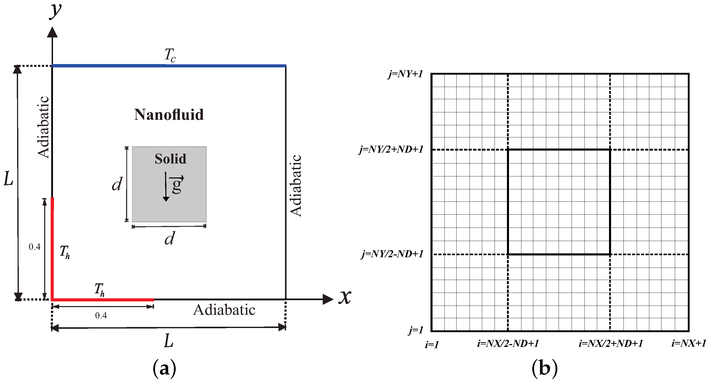
Figure 1 describes a schematic diagram related to the steady 2D natural convection in a square cavity (length
L) with a solid square insert (side
d) at the center. The selected range of Rayleigh numbers employed in this research keeps the flow of the nanofluid laminar and incompressible. Besides, a heater that is isothermal has been positioned at the bottom left in the cavity (length
), as portrayed by the thick red line, whereas the horizontal top wall had a constant cold temperature. The right vertical wall and the remaining areas of the heated walls are maintained as adiabatic. The annulus boundaries are presumed as impermeable toward the cavity fluid; Al
O
-water nanofluid. The Boussinesq approximation is applied. After weighing in the above assumptions, the momentum, continuity, and energy formulations for both steady and laminar natural convection can be written as follows:
where
refers to the velocity vector,
denotes the gravitational acceleration vector,
reflects the local volume fraction of nanoparticles and
stands for the nanoparticles mass flux.
The following depicts the energy equation for the inner solid wall.
Based on Buongiorno’s model, the nanoparticles mass flux is written as given below:
Now we describe the thermophysical properties of the nanofluid as the following:
The dynamic viscosity and thermal conductivity ratios of nanofluids (water-Al
O
) with 33 nm particle-size have been adapted according to Corcione [
12]:
where
is defined as:
where
(J/K) refers to Boltzmann constant.
nm reflects the fluid particles mean path.
denotes the water molecular diameter, as given by Corcione [
12]:
where
M stands for the base fluid molecular weight,
N is Avogadro’s number, and
denotes the base fluid density at standard temperature (310 K). With water as the base fluid, the value of
is obtained as follows:
The following presents the non-dimensional variables applied in this study:
This generates the dimensionless governing equations, as follows:
where
is the dimensionless velocity vector (
),
is the reference Brownian diffusion coefficient,
is the reference thermophoretic diffusion coefficient,
is Schmidt number,
is the diffusivity ratio parameter (Brownian diffusivity/thermophoretic diffusivity),
is Lewis number,
) is the Rayleigh number for the base fluid and
is the Prandtl number for the base fluid. The dimensionless boundary conditions of Equations (
20) and (24) are:
where
refers to ratio of thermal conductivity, and
stand for ratio of inner square cylinder width to outer square cylinder width.
The local Nusselt numbers examined for heated parts at the bottom and left walls are defined by:
Lastly, the average Nusselt numbers examined for heated parts of left and bottom walls are as follows:
and
3. Numerical Method and Validation
The iterative FDM was applied to find solutions to the dimensionless governing Equations (
20)–(24) subjected to boundary settings (
25)–(30).
Continuity and momentum equations in Cartesian coordinates are:
Continuity equation:
Momentum equation in the
X-direction:
Momentum equation in the
Y-direction:
Both stream function and vorticity are given as follows:
The stream function defined above automatically can satisfy continuity equation. Meanwhile, vorticity equation is generated after discarding the pressure built among these dual momentum equations by selecting the
Y-derivative of the
X-momentum and subtracting it from the
X-derivative of the
Y-momentum, hence yielding:
which simplified:
By using the definition of stream function, the following is obtained:
In terms of the stream function, the equation defining the vorticity becomes:
Since energy, volume fraction equation, and block conduction do not have pressure variable, the velocity in these equations can be easily transformed into stream function formulation.
The finite difference form of equation in relation to the dimensionless vorticity is as follows:
with
To obtain the value of
at the grid point of
, the values of
at the right must be retrieved first.
. This method is called the point Gauss-Seidel method, wherein the general formulation of this method is as follows:
The computation is assumed to move through the grid points from left to right, as well as from bottom to top. Here, superscript k refers to iteration number. The partition is applied as the solution domain in X-Y plane into equal rectangular sides and . The values of the relaxation parameter must be within the range for convergence. The range corresponds to under-relaxation, for over-relaxation, and denotes the Gauss-Seidel iteration. The finite difference form of equation linked to stream function, energy, and volume fraction can be treated in a similar manner.
The distribution of grid-points at the square cavity and adiabatic inner block is portrayed
Figure 1b, where
refers to node points in horizontal and vertical axes for adiabatic inner block. The temperature values for the left and bottom interfaces are given as follows:
Convergence for the solution is assumed when the relative error for each variable meets the convergence criteria listed below:
where
i denotes iteration number, and
refers to convergence criterion. The convergence condition was fixed at
in this study.
Several runs had been performed upon the grid in this study:
,
,
,
,
,
,
,
and
.
Table 1 presents the computed strength for circulation flow (
) as well as the average Nusselt number (
) for various grid sizes
,
,
and
. The findings displayed insignificant variances for
grids and above. Thus, the calculations presented in this study for similar problems depicted in this sub-section could employ the uniform gird of
.
As for data validation, the findings were compared with the outcomes reported in a prior publication Das and Reddy [
35] particularly for conjugate natural convection heat transfer in an inclined square cavity with a concentric solid insert, as illustrated in
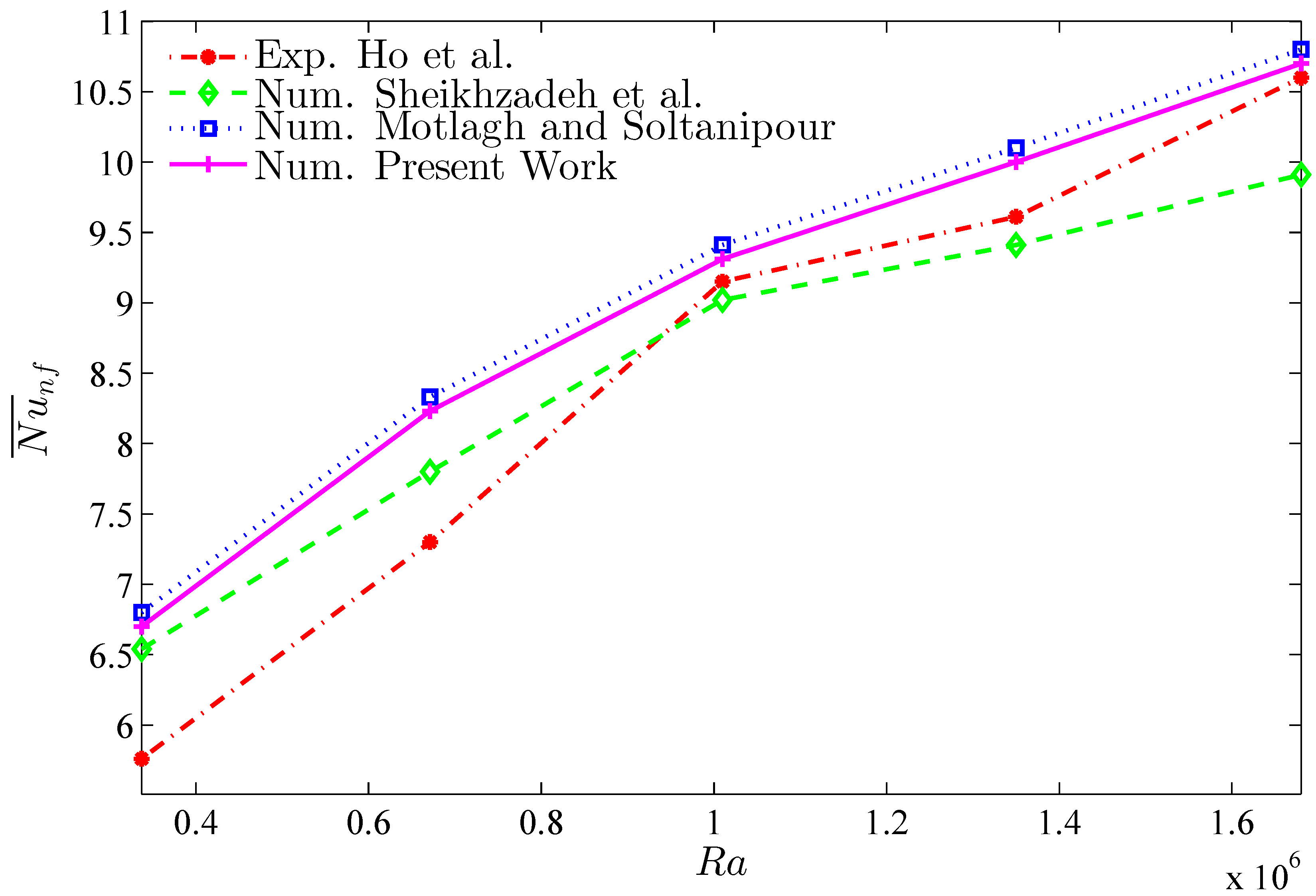
Figure 2. Additionally, a comparison was made for the average Nusselt number between the study outputs and those reported by Ho et al. [
36] (experimental outputs), Sheikhzadeh et al. [
37] (numerical outputs) and Motlagh and Soltanipour [
19] (numerical outputs) for depicting the natural convection of Al
O
-water nanofluid within a square cavity via Buongiorno’s two-phase model (see
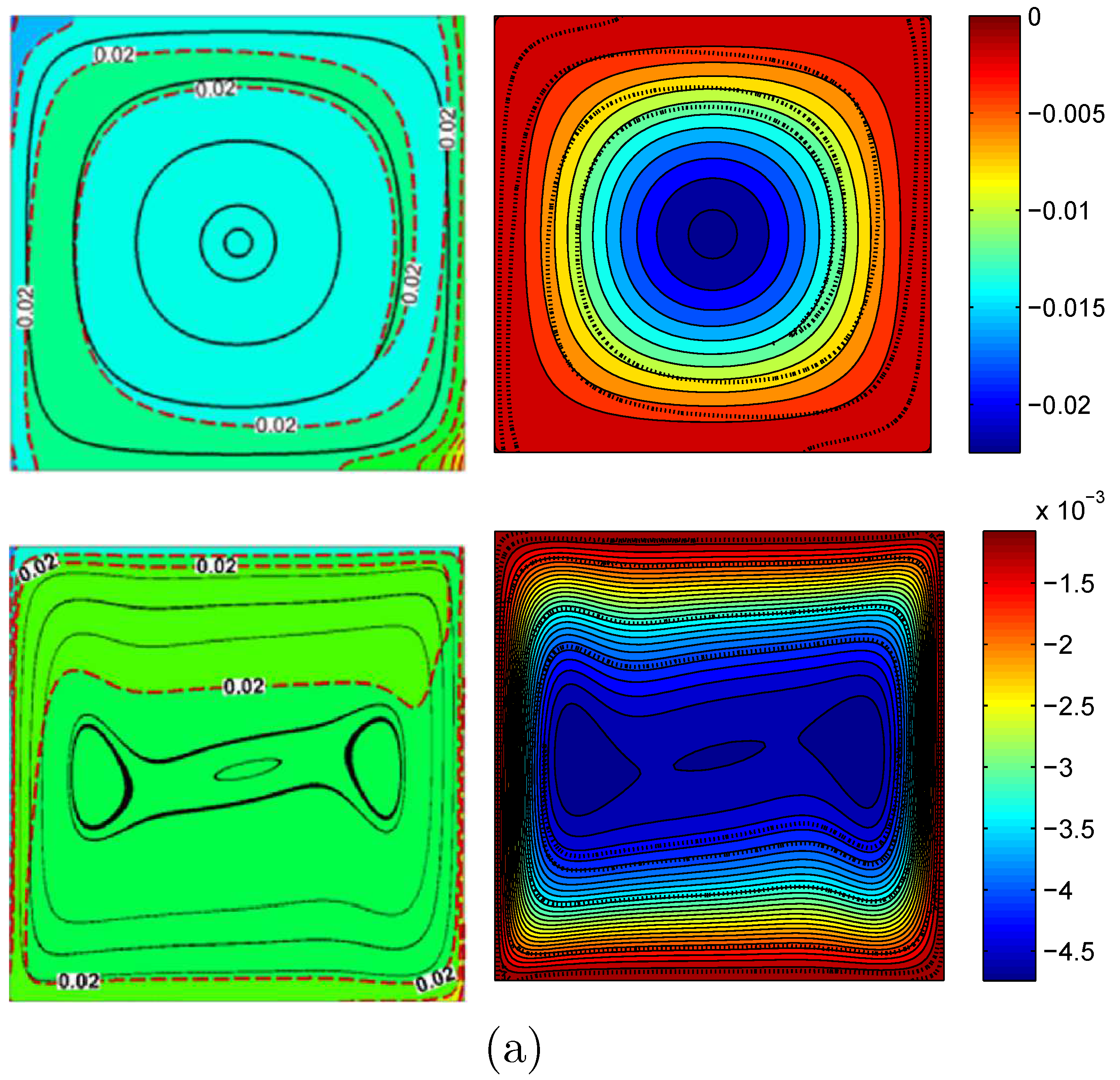
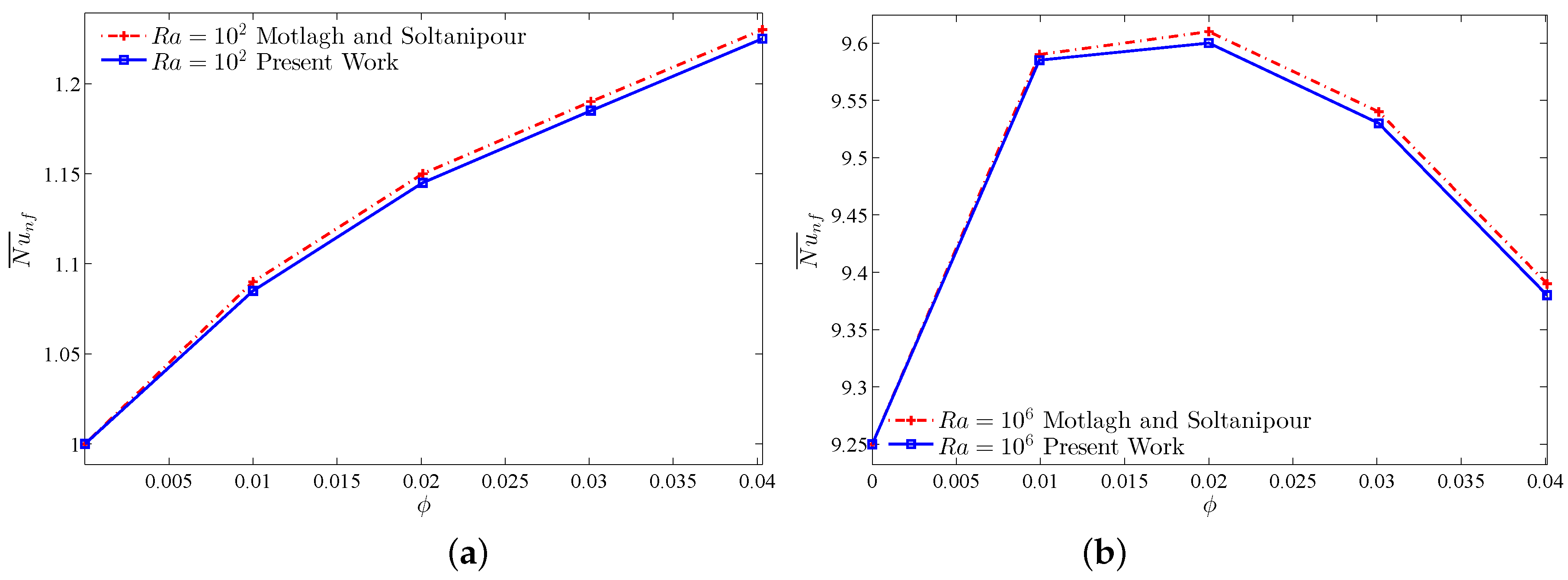
Figure 3). Another comparison was made between the study outcomes for the streamlines, isotherms, nanoparticles volume fraction, and the average Nusselt number results and those published by Motlagh and Soltanipour [
19], as illustrated in
Figure 4 and
Figure 5. The study outcomes appear to establish the validity and accuracy of the numerical approach.
4. Results and Discussion
This section presents the numerical outputs for the streamlines, isotherms, and the nanoparticles distribution, along with varied nanoparticle volume fraction values (
), the Rayleigh number
, thermal conductivity for conjugate square (
, 0.76, 1.95, 7 and 16) (epoxy: 0.28, brickwork: 0.76, granite: 1.95, solid rock: 7, stainless steel: 16), length of the inner solid (
) with fixed values for Prandtl number, Lewis number, Schmidt number, Brownian to thermophoretic diffusivity ratio, and normalized temperature parameter as follows:
,
,
,
, and
. The average Nusselt number was determined from various values of
and
D.
Table 2 presents the thermo-physical characteristics for both water (based fluid) and solid Al
O
phases.
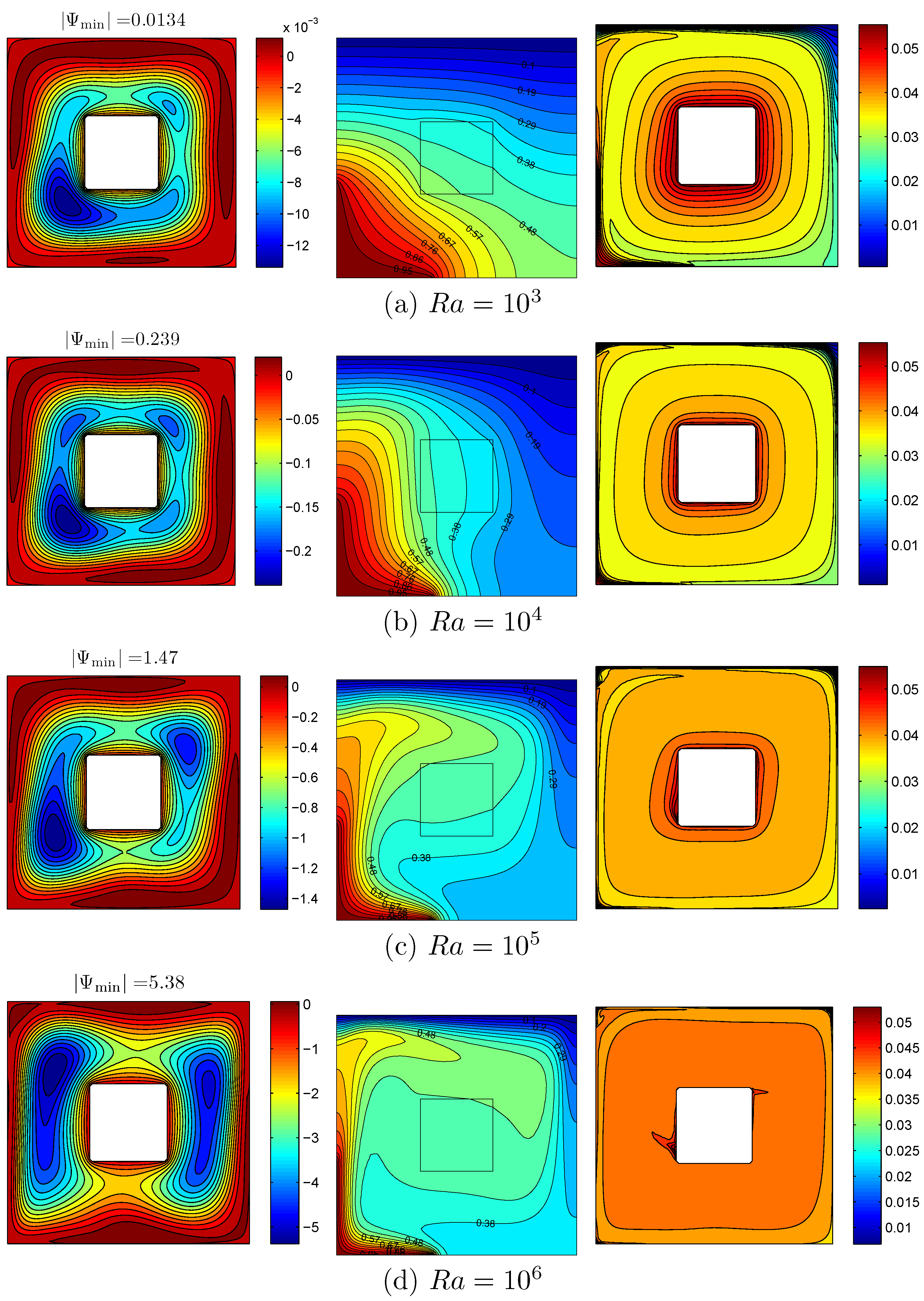
Legends of contour level reflect flow strength and direction of heated fluid (clockwise or otherwise). Positive values for refers to anti-clockwise flow and vice versa. denotes extreme values for stream function, which are vital to display minimum flow shift.
Figure 6 illustrates the impact of the volume fraction on the streamlines, isotherms, and the nanoparticles distribution at
, and
. For all runs, the streamlines display a huge cell that rotates clockwise around the solid block, which breaks down into double-core vortex wherein their centers are positioned at the cavity’s diagonal center. It also indicates the existence of dual secondary cells rotating in the direction of counterclockwise at right bottom and left top corners. The figure shows that the shape of the central regions in the main cells does not modify substantially although the average volume fraction of the nanoparticles is increased. The decrease in the streamlines magnitude signifies the increment of the nanofluid viscosity due to addition of solid nanoparticles. At this Rayleigh number, the contours of the isotherms exhibit that the isotherms gradient close to the horizontal cold wall in the enclosures increases steadily from the right section to the left part. Steep temperature gradients are noted near the heat sources. The figure also shows a minor increase in the gradient of the isotherms near the walls after raising the solid volume fraction. Based on
Figure 6, the particle distribution reflects the development of a mass boundary layer at the block walls. This occurs because the solid block impedes the fluid movement and traps the nanoparticles close to it. An increment of the average volume fraction adds to the boundary layer thickness, while the nanoparticle distribution becomes less uniform.
Figure 7 demonstrates the streamlines, isotherms and the nanoparticles distribution for the present configuration at
,
, and
to display the impact of the Rayleigh number
(from
to
) upon the flow, thermal, and the concentrations fields. It is evident that at a small Rayleigh number, the isotherms exhibit parallel dispersion at the horizontal wall that is cold, thus indicating the dominance of conduction mode in transfer of heat. An increment in the Rayleigh number leads to a stronger convection heat transfer, a steeper cold wall, and adjacent temperature gradients to the edges of the heaters, thus augmenting the Nusselt numbers within these regions. The isotherms in the block are almost parallel, hence indicating that heat is transmitted via conduction through the solid block and tilted in the clockwise direction with increasing values of the Rayleigh number. With greater Rayleigh numbers, the central core vertices for the main cell shifts from circular to oval shape and further moves to be vertical within the cavity at
. The flow strength increases to indicate enhanced force of buoyancy that overcomes the viscous force, in which convection dominates transfer of heat. The isoconcentration contours show that with a low Rayleigh number, the heat transfer via conduction becomes dominant and thermophoresis displays a strong influence on the distribution of nanoparticles inside the cavity (thermophoretic effects that move solid nanoparticles to cold regions from hot areas). Thus, the nanoparticles showcase non-uniform dispersion within the cavity, along with an essential increase in the nanoparticles concentration near the block walls. At high Rayleigh numbers, the distribution of nanoparticles turns fairly uniform due to the strength of the buoyancy effects that trap more nanoparticles at the recirculation zones, which cause less deposition of nanoparticles. Thus, the single-phase homogeneous approach can be used for this stage.
Figure 8 presents the streamlines, isotherms, and the nanoparticle distributions at specific values of
,
and
, in comparison to various values of the thermal conductivity of the solid block. After increasing
, the block isotherms become sparser as the heated fluid that flows in the upper channels transfer a large portion of heat to the cold fluid at the lower channel through the conducting solid block. The flow intensity decreases slightly with increasing values of the thermal conductivity of the block. This can be explained by the fact that by elevating the thermal conductivity in the block, the flowing cold fluid at the lower channel within the enclosure gets more heated by the block instead of the heated corner walls, thus reducing the overall heat transfer via natural convection between the cavity walls in an effective manner. In addition, the layer of mass boundary near the block walls grows by increasing the thermal conductivity of the block, and therefore, the nanoparticles distribution within the cavity is weakly homogeneous with large values of
. This occurrence is estimated due to the impact of increasing
advection.
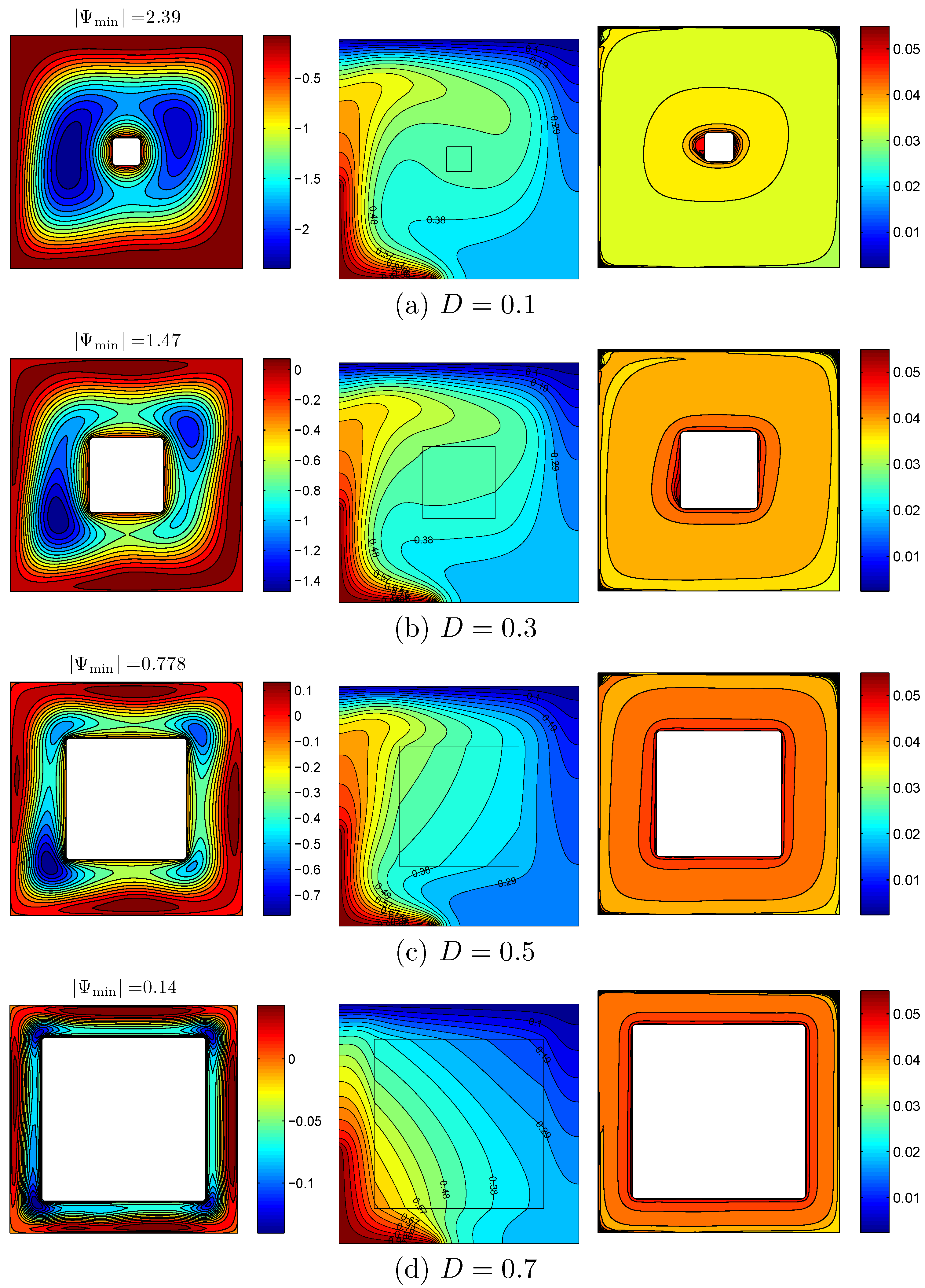
Figure 9 displays the impact of the block size upon flow behavior, in which
and
. Obviously, the increasing length of ratio
D leads to smaller space for the flow to circulate and consequently, a decrease in the magnitude of the streamlines and the natural convection flow turns weaker. It is observed that by increasing the block size, the isotherms lines became less dense at the cavity active walls, which reduced the Nusselt number. Nanoparticles distribution contours illustrate that the increment in uniform dispersion with the increment of the block size is mainly due to a geometric reason that narrows the flow area.
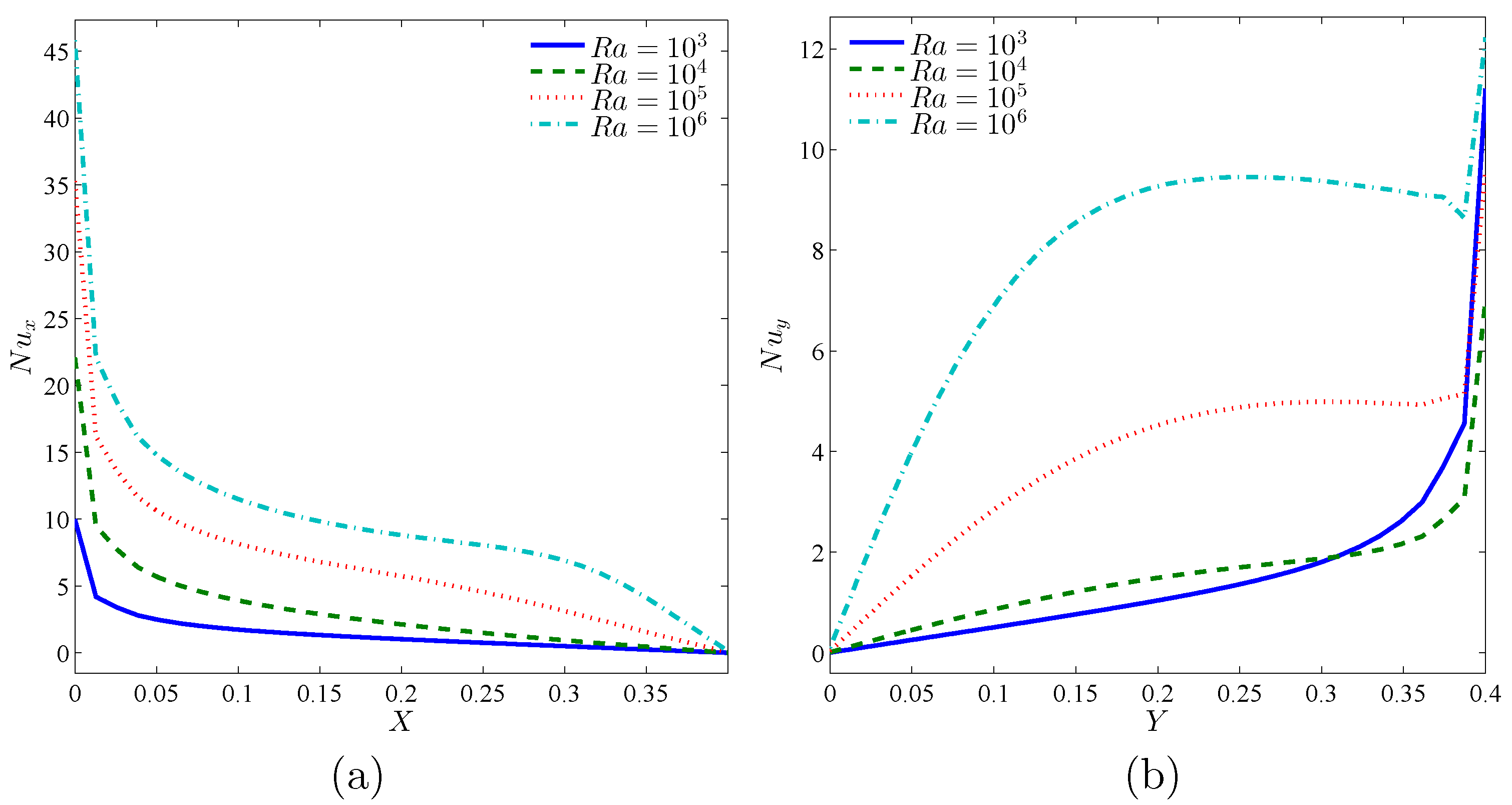
Figure 10 illustrates the variation of the local Nusselt numbers for the vertical and horizontal surfaces at the corner heater with various Rayleigh numbers
at
and
. The local Nusselt number increases monotonically at the vertical heater, but decreases at the horizontal one in accordance to the development of the temperature gradient on the heaters. As expected, an increment in the Rayleigh number increases the local Nusselt numbers. The figure portrays that the minimum values depicted at the center of corner are unaffected by the Rayleigh number, substantial increments of the local Nusselt numbers have been noted as the Rayleigh numbers hike at the edges of the heaters. Besides, the values of the Nusselt number on the vertical heater are much affected due to the Rayleigh number. In fact, increasing the Rayleigh number causes the left vortex core to grow vertically closer to the vertical heater and consequently, enhances the heat transfer rate at this particular area.
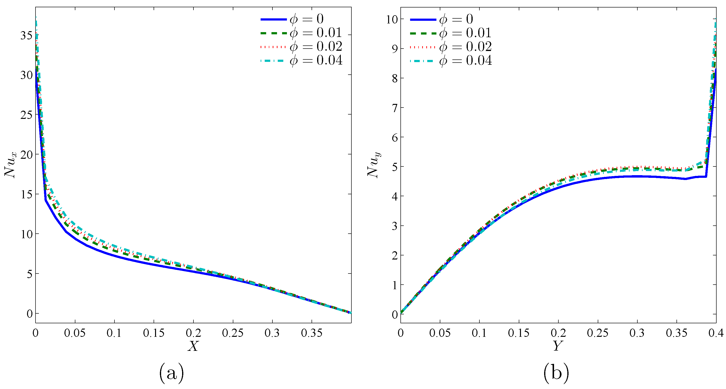
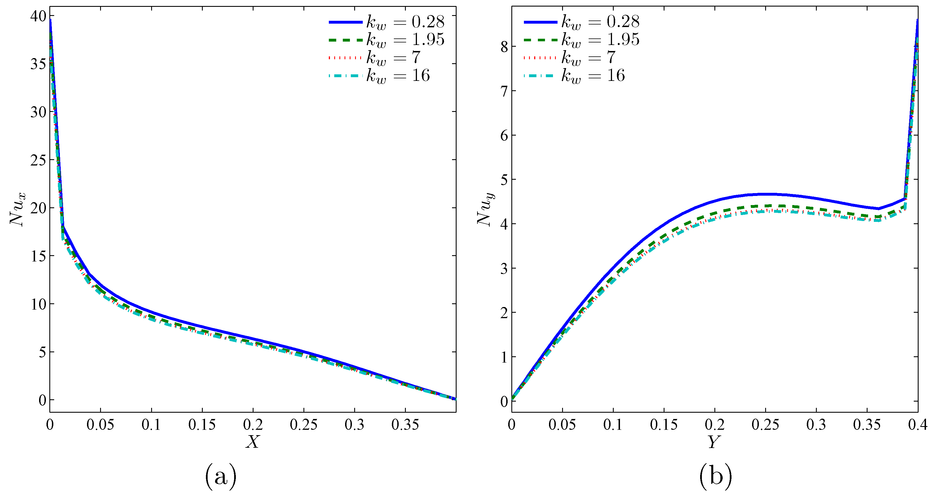
The slight increment of the local Nusselt numbers, as shown in
Figure 11 and
Figure 12, seem parallel with the increasing average volume fraction of nanoparticles (
Figure 11) and decreases slightly due to increment in the block thermal conductivity (
Figure 12). The reason for this is mainly because when the ratio of the thermal conductivity
is increased (increasing
decreasing
), a substantial fraction of heat from the heated fluid at the upper channel is transferred through the block to heat the cold fluid flowing at the lower channel, rather than transporting heat to the cold cavity walls, and the flowing cold fluid at the lower channel is heated by the block instead of the heaters. This mechanism decreases the rate of heat transfer via natural convection.
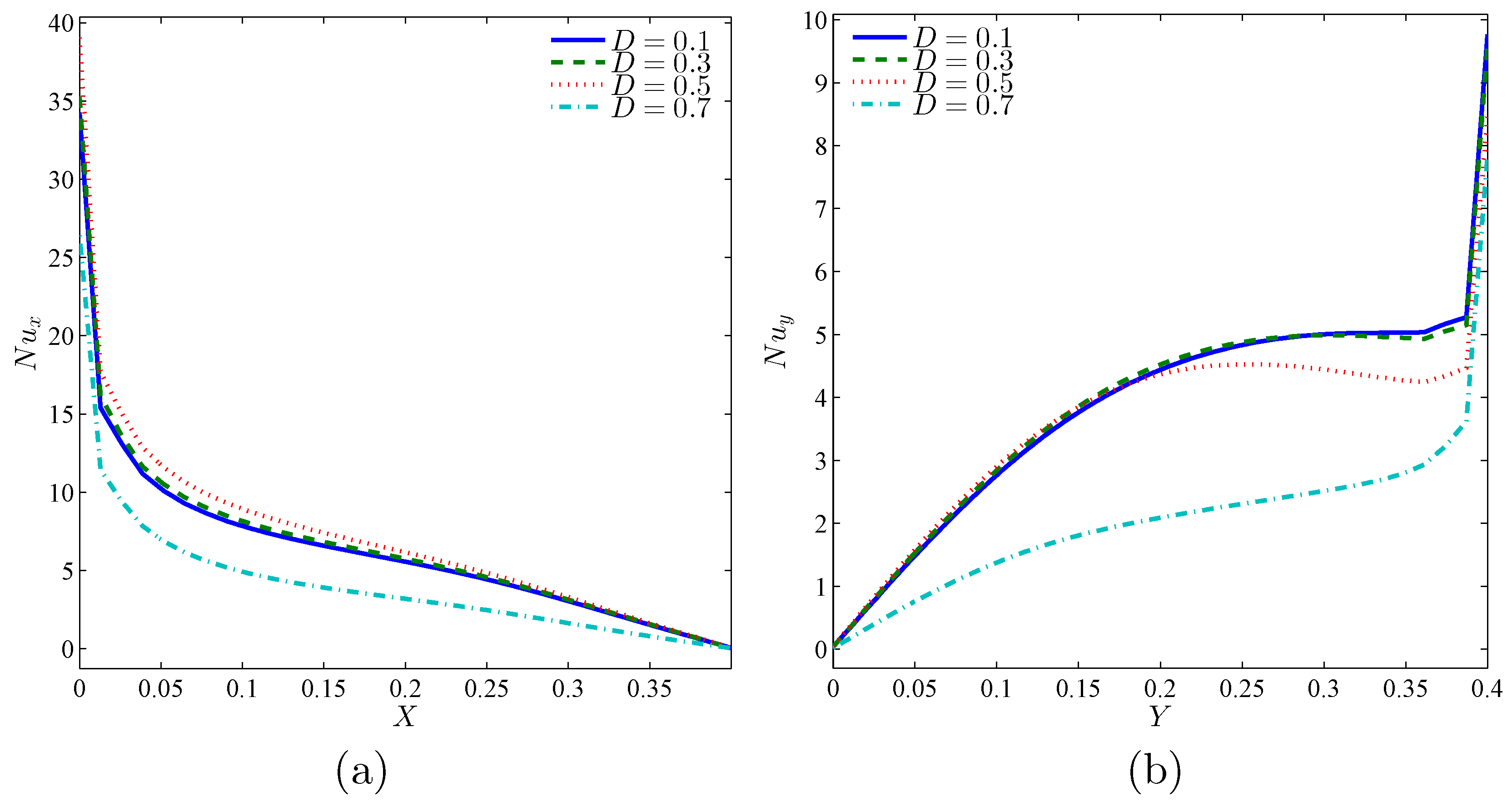
Figure 13 shows the maximum value for block size (
) after reduction in Nusselt numbers with
D for horizontal heater. The values of Nusselt decreased on the vertical heater with increment in
D.
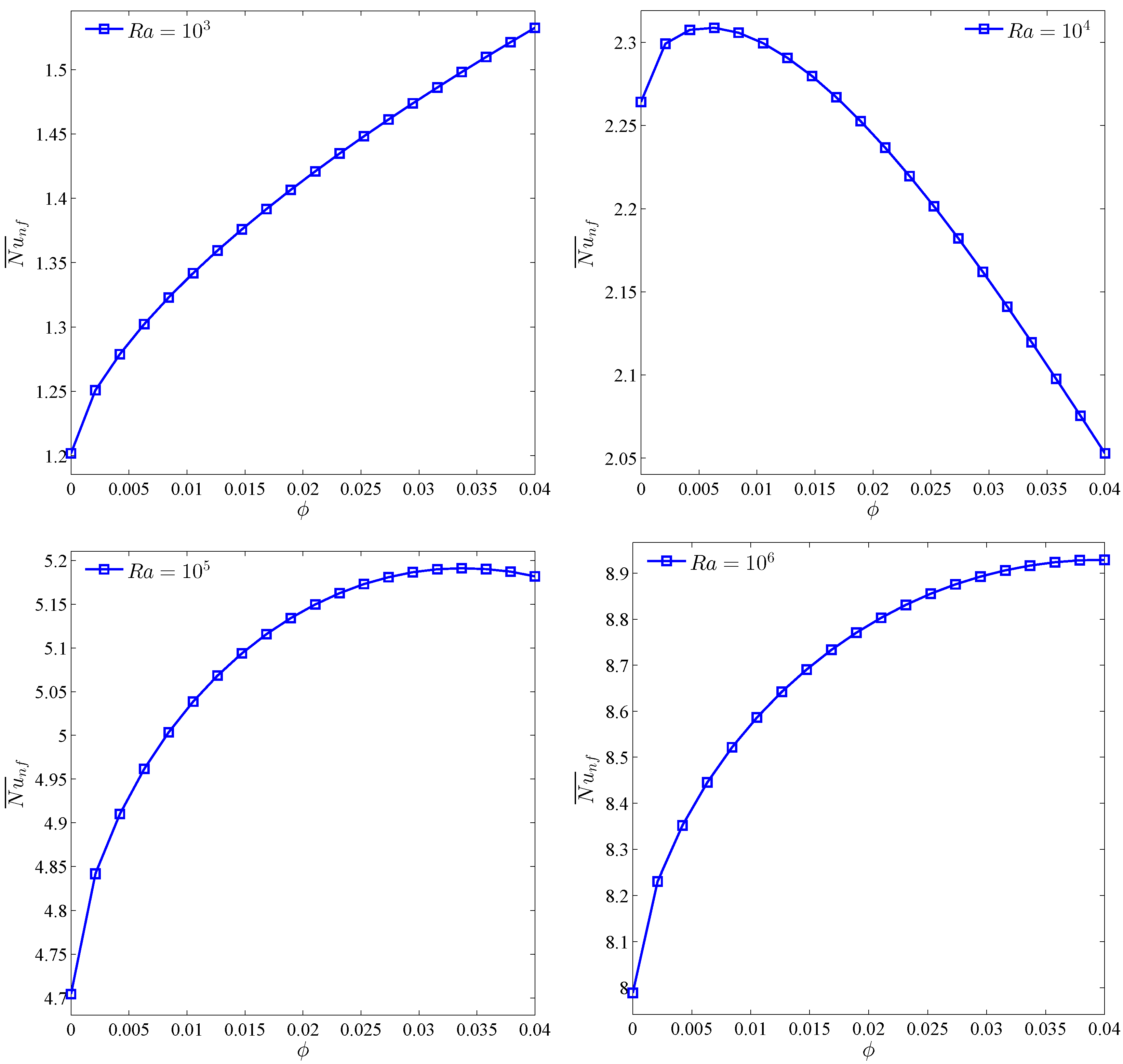
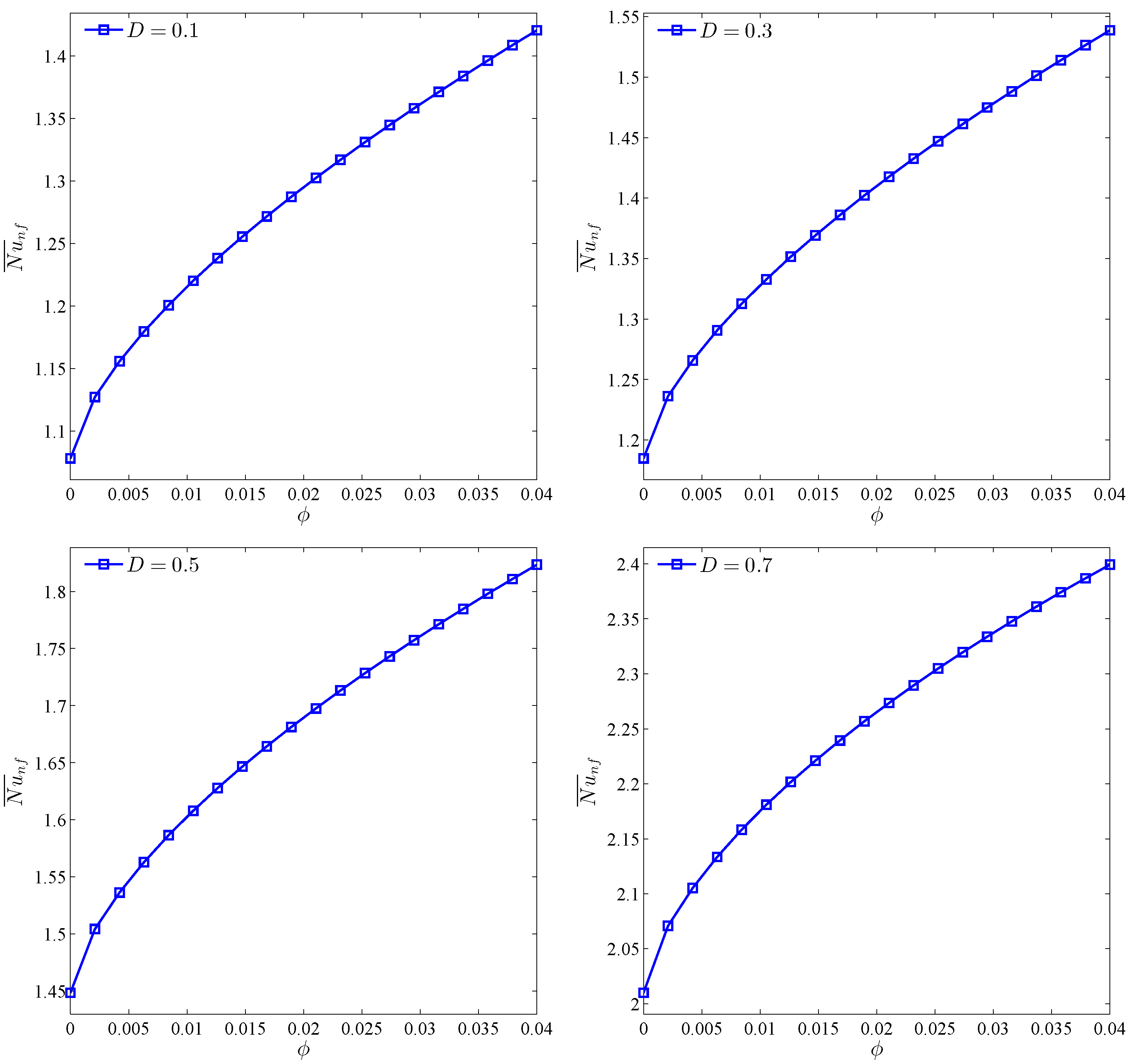
Figure 14 portrays the mean value of the Nusselt number, in comparison to the nanoparticles volume fraction at each Rayleigh number separately when
and
. At a low Rayleigh number (
), the Nusselt number continually increases with an increment in the nanoparticles volume fraction, whereas at
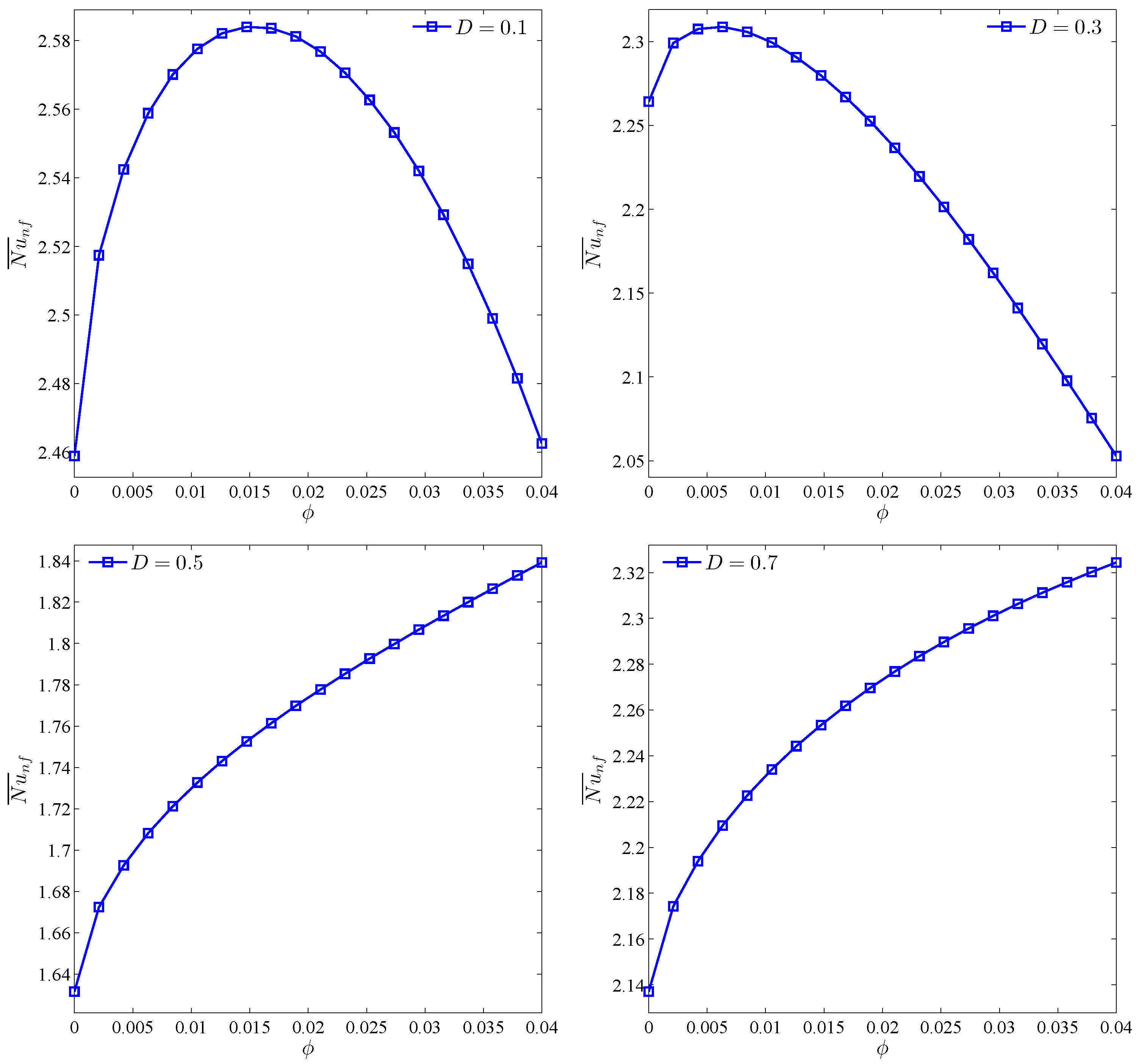
, an optimum concentration of nanoparticles is observed for the maximum mean value of the Nusselt number. This is because; inclusion of nanoparticles enhances both the fluid viscosity and the fluid thermal conductivity. The combination of these dual effects optimizes the concentration of the nanoparticle for a maximized rate of heat transfer. Furthermore, when the Rayleigh number is increased, the maximized average Nusselt number values move to higher values of the nanoparticles volume fraction.
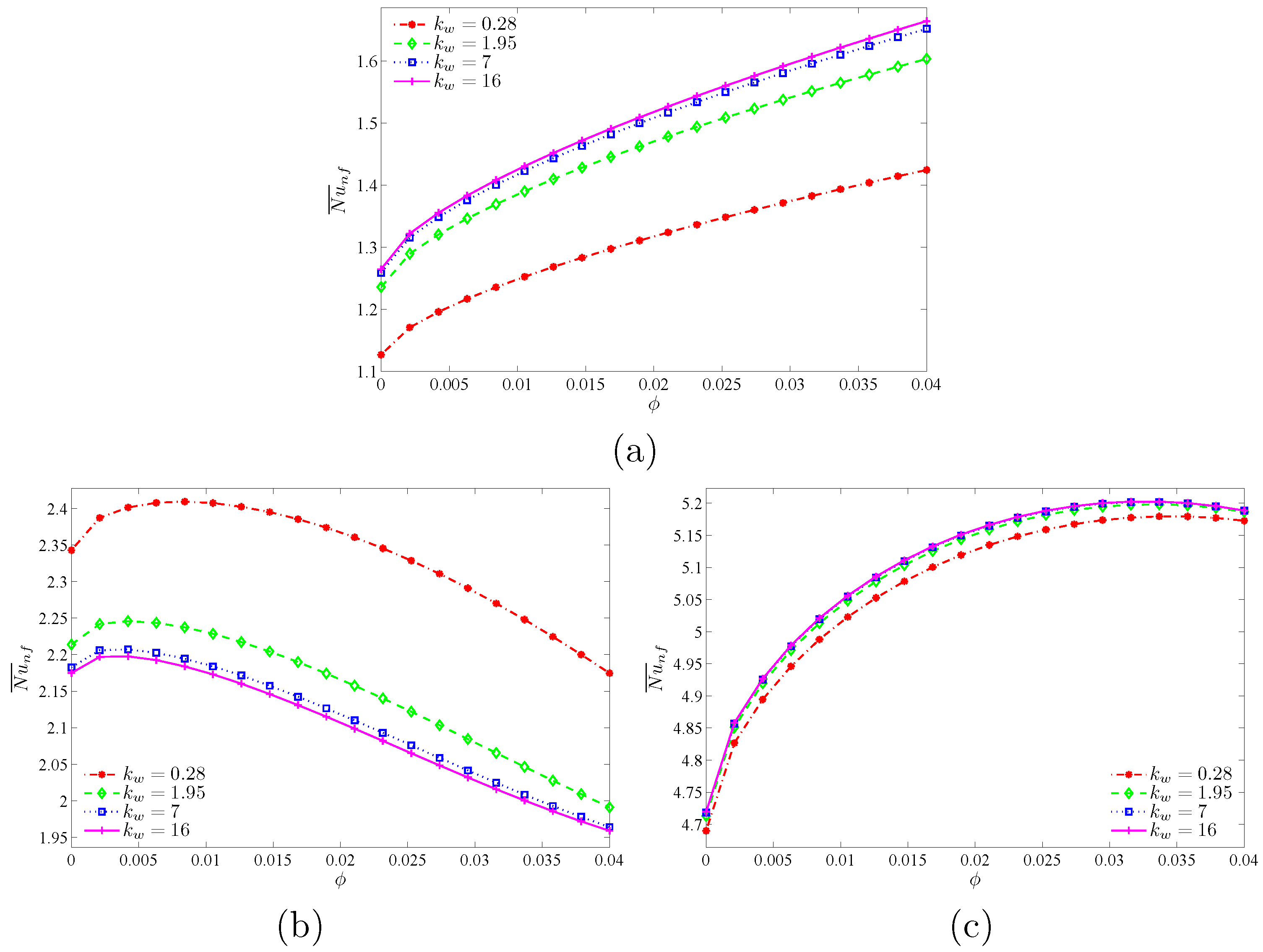
As for the block size, the impact of the block thermal conductivity seem to be positive on heat transfer when the Rayleigh number is low, wherein the primary mode for transfer of heat is conduction. A higher block thermal conductivity decreases the rate of heat transfer, particularly for moderate Rayleigh numbers. Since a stronger convection has an impact upon high Rayleigh numbers, the influence of Kw weakens, when compared to the buoyancy forces, in which one can gain an opposite effect (see
Figure 15).
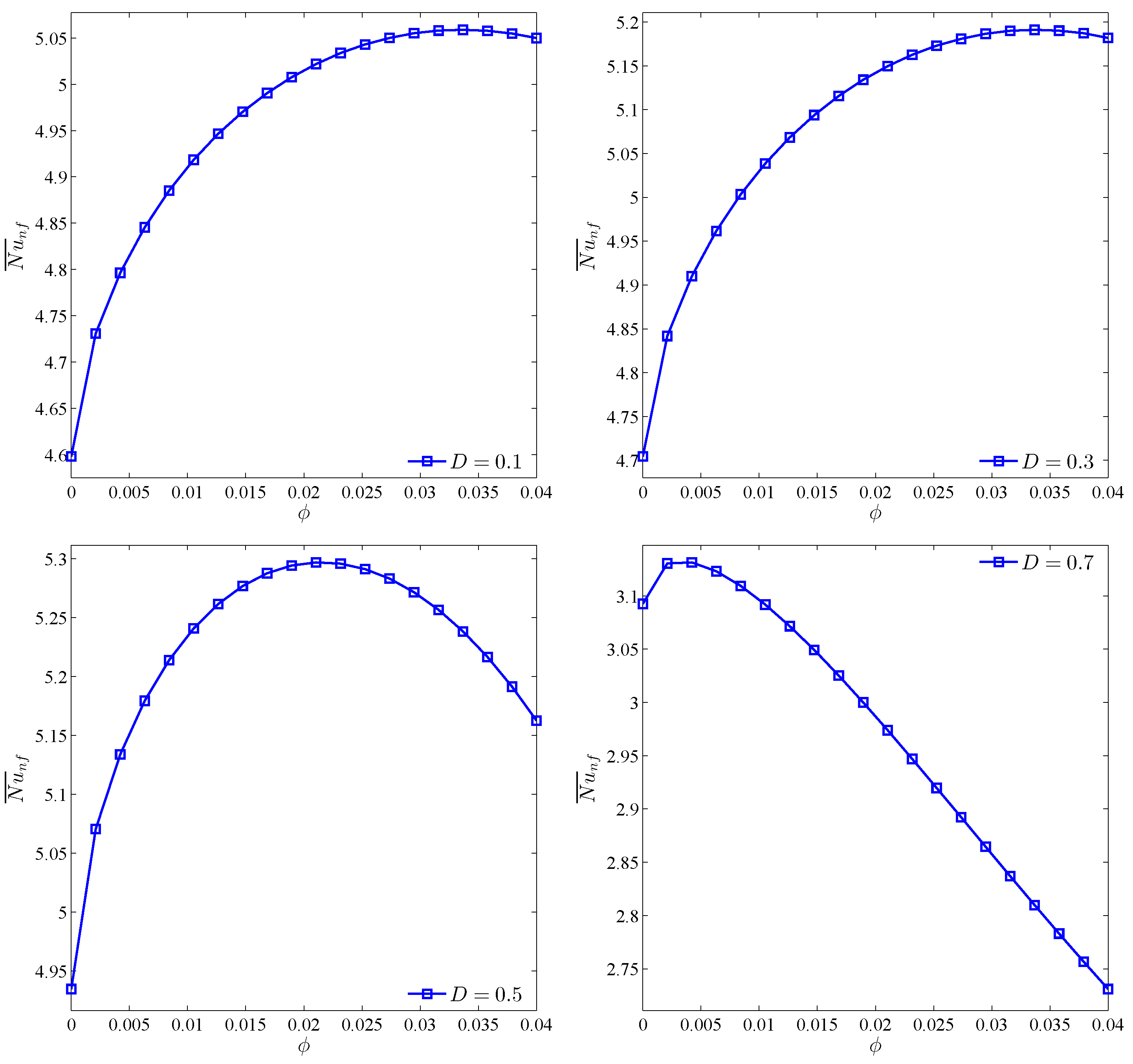
Figure 16,
Figure 17 and
Figure 18 illustrate the varied values of the average Nusselt number with mean volume fraction at each block size, as well as the Rayleigh number for the same thermal conductivity block (
). As discussed earlier, when conduction dominates heat transfer (at
), the Nusselt number appears to hike monotonically, along with the mean for the nanoparticles volume fraction. For a given volume fraction; the Nusselt numbers seem to increase after elevating
D because the increase in the block size reduces the flow of natural convection. At
(
Figure 17), several optimal values are noted for the mean value of the Nusselt number, particularly for
. Since the block size weakens natural convection, the natural convection is suppressed at
. Nonetheless, the Nusselt returns to increase continually with
, as well as by increasing
D for a given volume fraction. As observed in
Figure 18, large Rayleigh numbers generate maximum average Nusselt number values, which shift to low values for the nanoparticles volume fraction by increasing
D.
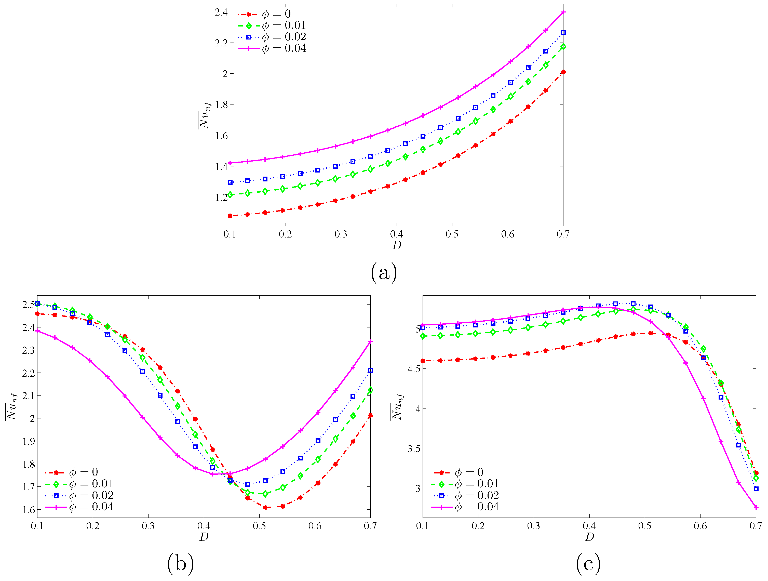
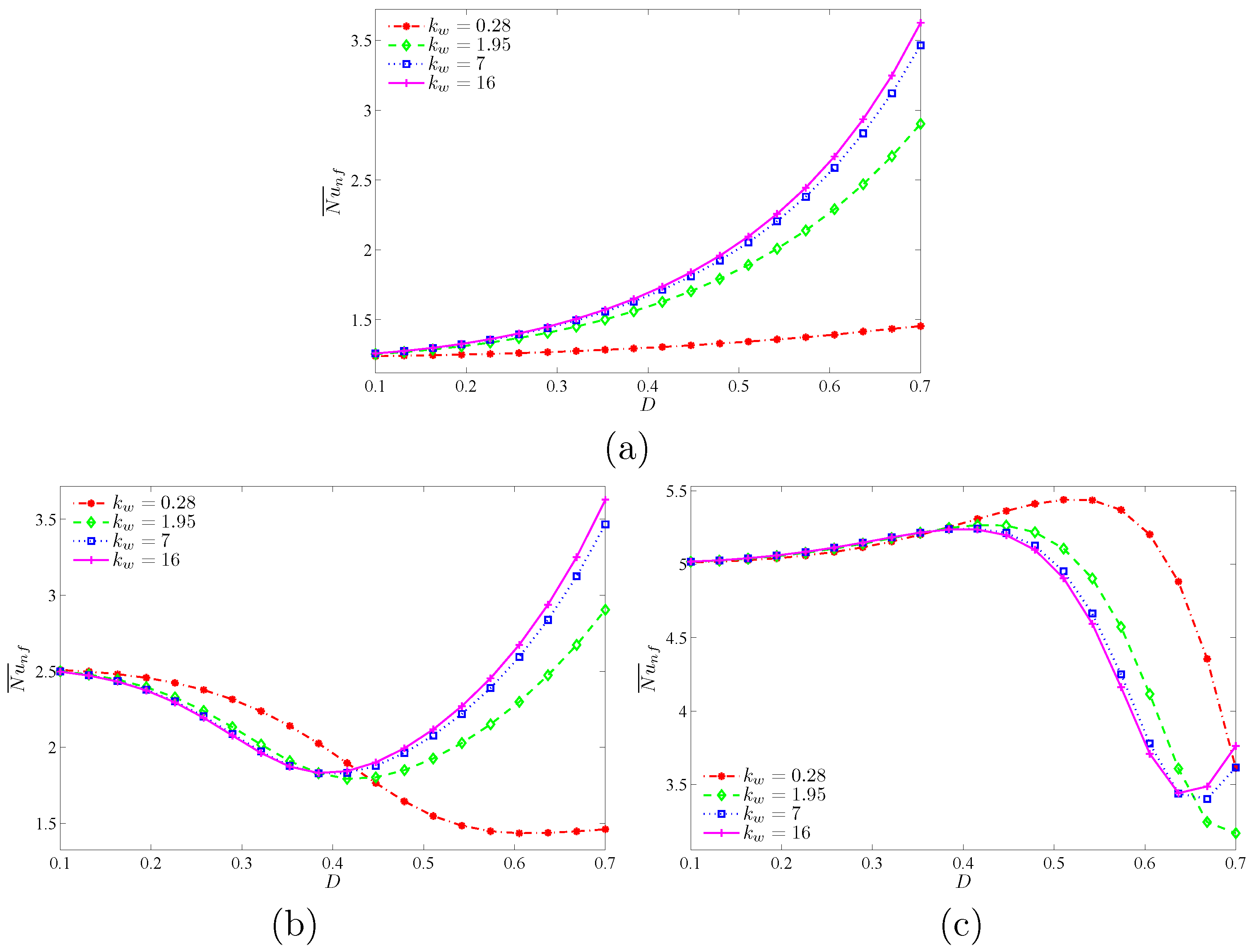
For a better comparison,
Figure 19 illustrates the varied values of the average Nusselt number, along with
D for differing volume fraction values at
; (a)
, (b)
and (c)
. Based on
Figure 16, at a low Rayleigh number, the mean value of the Nusselt number increases by increasing the block size for all ranges of
. At a moderate Rayleigh number and all
values, first, the Nusselt number reduces to attain its minimum, and then increases monotonically. This minimum Nusselt number seems to correspond to smaller block size, when compared to the size that manages to suppress the flow in natural convection. The
D value that suppresses the flow of natural convection reduces after increasing
. For a larger Rayleigh number, when the convection is stronger, the Nusselt number first increases slightly to reach a maximum, and later, decreases monotonically. The maximum also corresponds to the
D value, wherein the block begins to substantially suppress the flow of natural convection.
As portrayed in
Figure 20, when the Rayleigh number is low, the transfer of heat is improved due to the increment in the block thermal conductivity. This actually refers to a reverse impact as the convection dominates until the
D value is obtained upon suppression of the natural convection flux by the block. This is mainly due to the thermal leakage by conduction through the block, which strengthens the heat transfer rate, in which conduction dominates the transfer of heat (high diffusion) and the opposite appears to be true with the existence of natural convection (small diffusion). It is clear from
Figure 20c, that with a high Rayleigh number and increased value of
are sufficient to attain the value of
D, wherein the block can successfully suppress the free convective flow.


