Simplified Analytic Approach of Pole-to-Pole Faults in MMC-HVDC for AC System Backup Protection Setting Calculation


State Key Laboratory of Advanced Electromagnetic Engineering and Technology, Hubei Electric Power Security and High Efficiency Key Laboratory, School of Electrical and Electronic Engineering, Huazhong University of Science and Technology, Wuhan 430074, China
*
Author to whom correspondence should be addressed.
Energies 2018, 11(2), 264; https://doi.org/10.3390/en11020264
Submission received: 29 November 2017
/
Revised: 19 January 2018
/
Accepted: 19 January 2018
/
Published: 23 January 2018
(This article belongs to the Section F: Electrical Engineering)
Abstract
:AC (alternating current) system backup protection setting calculation is an important basis for ensuring the safe operation of power grids. With the increasing integration of modular multilevel converter based high voltage direct current (MMC-HVDC) into power grids, it has been a big challenge for the AC system backup protection setting calculation, as the MMC-HVDC lacks the fault self-clearance capability under pole-to-pole faults. This paper focused on the pole-to-pole faults analysis for the AC system backup protection setting calculation. The principles of pole-to-pole faults analysis were discussed first according to the standard of the AC system protection setting calculation. Then, the influence of fault resistance on the fault process was investigated. A simplified analytic approach of pole-to-pole faults in MMC-HVDC for the AC system backup protection setting calculation was proposed. In the proposed approach, the derived expressions of fundamental frequency current are applicable under arbitrary fault resistance. The accuracy of the proposed approach was demonstrated by PSCAD/EMTDC (Power Systems Computer-Aided Design/Electromagnetic Transients including DC) simulations.
1. Introduction
AC (alternating current) system protection setting calculation is an important basis for ensuring the safe operation of power grids. The backup protection setting calculation, which has to take protection coordination into consideration, is the most complicated and time-consuming part. Studies on backup protection setting calculation have been maturing with the expansion of AC power grids over the last few decades [1,2,3,4,5].
Recently, with increasing carbon dioxide emissions and fossil energy shortages, renewable energy has drawn more attention. As the integration of renewable energy depends on a more efficient, reliable, and flexible electric transmission technology, voltage source converters based on high voltage direct current (VSC-HVDC) have been widely investigated [6,7,8]. These include two-level and three-level VSC-HVDC, and multi-level modular converter (MMC) HVDC. Compared to the two-level and three-level VSC-HVDC, MMC-HVDC has advantages of lower harmonics and higher modularity [9,10,11], and is one of the most promising HVDC technologies. Several MMC-HVDC projects are in operation or under planning around the world [12,13].
Under pole-to-pole faults, the AC system feeds the fault current through the anti-parallel diodes of MMC arms even when the MMC is blocked [14,15,16]. AC circuit breakers are employed to clear the faults in most of the practical projects, as DC circuit breakers have yet to be widely utilized commercially [16,17]. If a AC circuit breaker malfunctions, the fault needs to be detected and cleared by the upstream protection devices. This kind of fault clearing method in MMC-HVDC has influenced the AC system backup protection setting calculation, to the extent that the impact cannot be ignored, as more MMC-HVDCs with higher capacity and voltage level are being integrated into power grids. However, AC system backup protection setting calculation is usually implemented in the systems that contain massive nodes and operation modes. Simplified analytic approach of faults is preferred for improving the efficiency of the setting calculation, instead of the EMTDC simulation approach [18,19,20], which is complicated in modeling and computation. Therefore, it is essential to develop a simplified analytic approach of pole-to-pole faults in MMC-HVDC for the AC system backup protection setting calculation.
Bucher et al. [21] developed an analytic approximation of fault current contribution from AC networks to symmetric bipolar MTDC (multi-terminal DC) networks during pole-to-ground faults, which was based on the assumption that three diodes conduct simultaneously after the MMC has been blocked. These kinds of faults are the same as pole-to-pole faults in symmetric monopole. Li, B. et al. [22] carried out the DC fault analysis for a MMC-HVDC system. It was concluded that there was a commutation overlapping phenomenon in the blocked MMC due to the existence of arm reactors, which meant that the number of conducting diodes varied under different fault conditions. Li, C.Y. et al. [23] presented a pole-to-pole fault current calculation method for DC grids on the premise that the MMC was not blocked. He et al. [24] investigated the distance protection of AC gird with HVDC-connected offshore wind generators under AC-side short-circuit faults that are close to points of common coupling (PCCs), and presented an apparent impedance calculation method. Liu et al. [25] developed an adaptive distance relay based on the measurement information on PCCs of MMC-HVDC under AC-side short-circuit faults, which could reduce the adverse impact on the AC line distance relay. In summary, the recent literature has mainly focused on the DC-side electrical quantities, while the AC-side electrical quantities that the AC system backup protection setting calculation is concerned with, especially those for pole-to-pole faults, are rarely involved.
In this paper, a simplified analytic approach of the pole-to-pole faults in MMC-HVDC for the AC system backup protection setting calculation is proposed. Two concepts, critical resistance and critical state, were defined to clarify the analysis of the fault process. Current loops and boundary conditions of the critical states were determined. Based on the critical states, the linear combination method was employed to derive the expressions of fault current, applicable under arbitrary fault resistance. The MMC-HVDC systems were modeled in PSCAD/EMTDC (Power Systems Computer-Aided Design/Electromagnetic Transients including DC) to validate the accuracy of the proposed approach.
This paper is organized as follows: Section 2 presents the principles of pole-to-pole fault analysis. Section 3 investigates the influence of fault resistance on pole-to-pole faults. The simplified analytic approach for AC system protection setting calculation is proposed in Section 4. Section 5 shows the validation of the proposed approach. The conclusions are drawn in Section 6.
2. Principles of Pole-to-Pole Fault Analysis
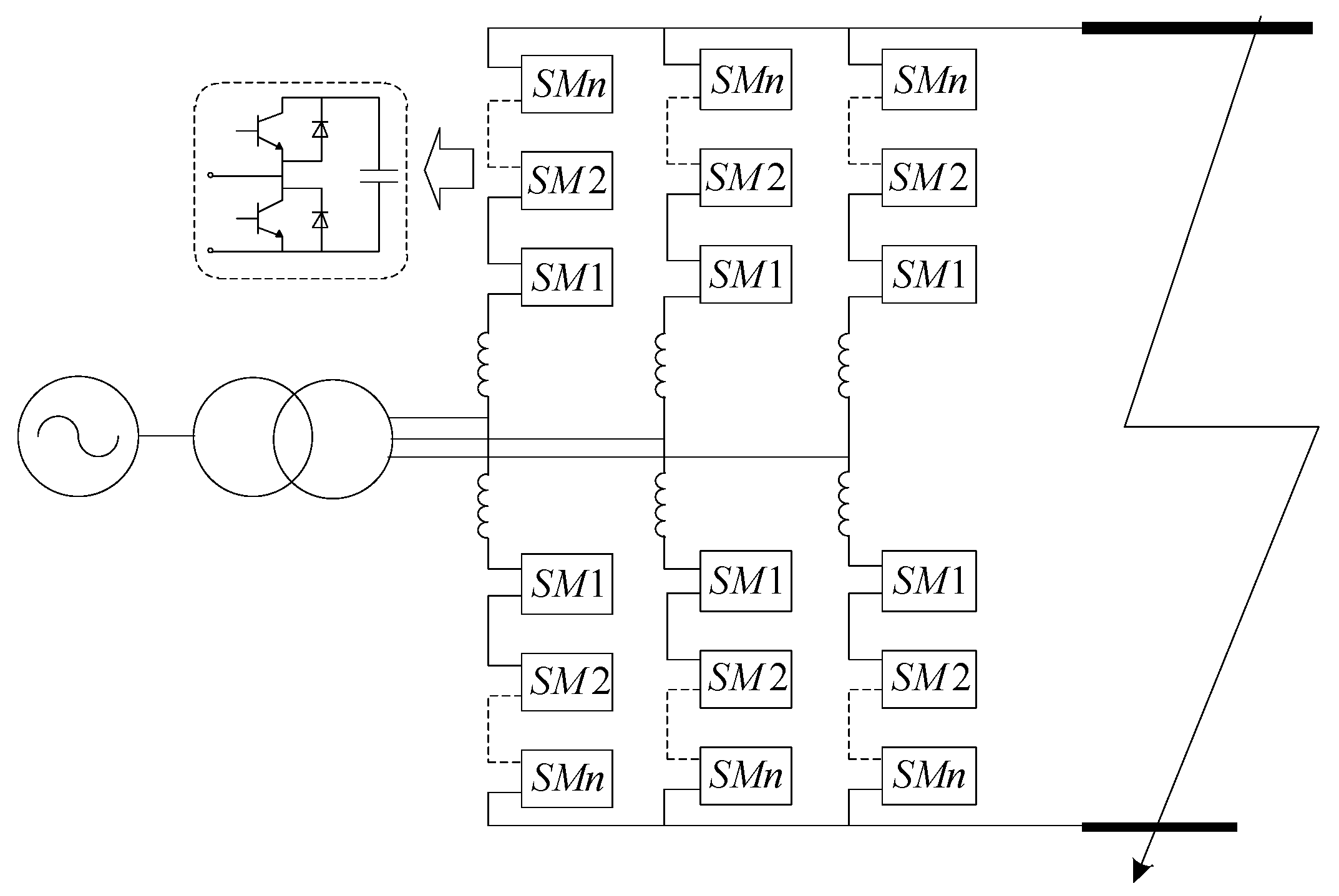
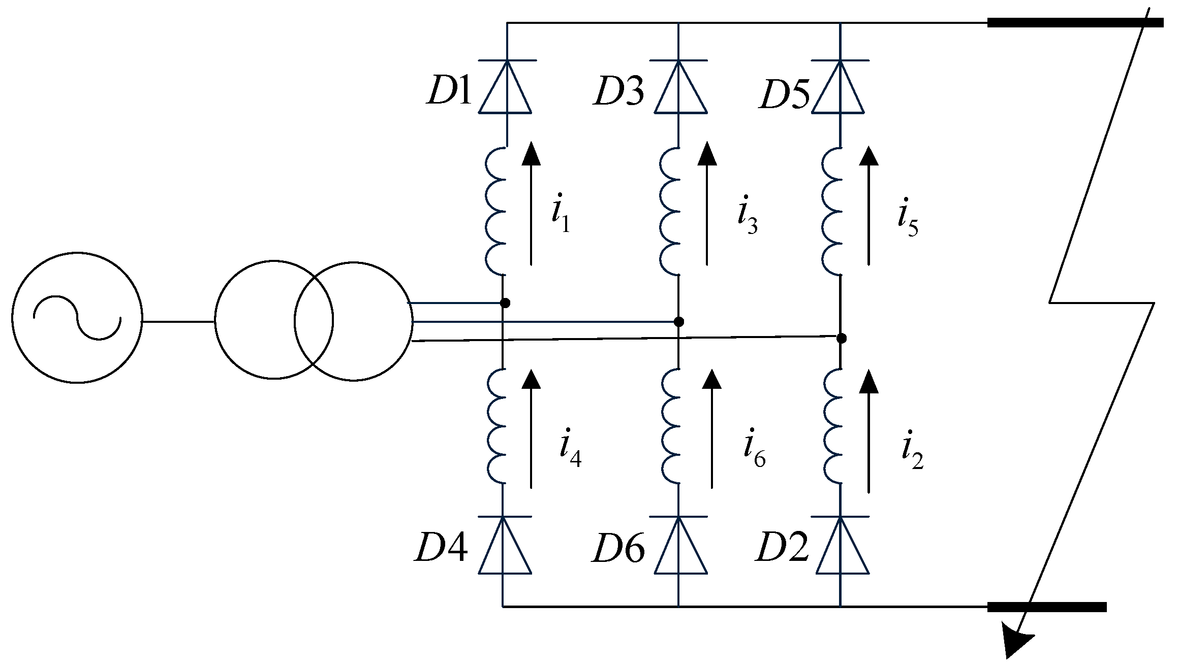
A schematic diagram of pole-to-pole faults in MMC-HVDC is shown in Figure 1. The fault process can be divided into two states. (1) Transient state: When the fault occurs, the DC voltage drops rapidly and the capacitors in the sub-modules discharge, leading arm current to rise. Then, the MMC is blocked after milliseconds [16], and the capacitors are bypassed to prevent the insulated gate bipolar transistors (IGBTs) from being damaged by the rising arm current. The blocked MMC is equivalent to a three-phase uncontrolled rectifier, as shown in Figure 2. The arm current in (n = 1, 2, …, 6) attenuates as the capacitors are bypassed, leading to the un-periodic conduction of diodes Dn (n = 1, 2, …, 6). The variation of fundamental frequency current shows non-periodicity. (2) Steady state: When the attenuation process of the arm current is finished, the steady state begins. In this state, the diodes conduct periodically, consequently, the variation of fundamental frequency current shows periodicity. The steady state will last until the AC circuit breaker operates.
In the pole-to-pole fault process, the duration of the transient state is remarkably shorter than the AC system backup protection setting time [26], which is usually hundreds of milliseconds. The reason is that the capacitors are not fully discharged when the MMC is blocked after milliseconds, and consequently the arm current attenuation process, which corresponds to the discharging of capacitors, only lasts for tens of milliseconds in general. Figure 3 shows the AC current under pole-to-pole faults, where iac is the AC current, and Ip50Hz is the peak value of the fundamental frequency current. It was observed that Ip50Hz became constant after about 30 milliseconds, which meant that the transient state had ended.
Moreover, the standard of AC system protection setting calculation [26] stipulates that ignoring the non-periodic component and periodic component attenuation in the AC current is allowable to simplify the setting calculation. Therefore, the principles of pole-to-pole fault analysis for the AC system backup protection setting calculation can be concluded as follows:
- Only the steady state is considered.
- Only the fundamental frequency current is considered.
It is worth noting that the RMS (root mean square) component calculation in relays usually requires a half or a full cycle. However, the fundamental frequency current becomes constant after about 30 milliseconds, as aforementioned. Therefore, the time delay due to the RMS calculations in relays does not affect the analysis and can be ignored.
3. Influence of Fault Resistance on Pole-to-Pole Faults
In the steady state, the blocked MMC is also equivalent to a three-phase uncontrolled rectifier, as shown in Figure 4. E and Em(a,b,c) are the AC source voltage and mid-arm voltage, respectively. Ls is the inductance of the arm reactor. Rf and Lf are the resistance and inductance at the DC side, called the fault resistance and fault inductance, respectively. idc and iac are the DC current and AC current, respectively. Lt is the equivalent inductance of the transformer. To better illustrate the analysis, the AC system was equivalent to a voltage source. It is worth noting that the protection in this paper is the AC system backup protection. That is, if Bp fails to trip when pole-to-pole fault occurs, the AC circuit breakers Bbk (k = 1, …, K) will be tripped as the backup protection. Therefore, the measurements used by the backup protection we investigated are at the remote ends of the lines feeding the transformer.
The AC system feeds the fault current through the uncontrolled rectifier continuously. However, this uncontrolled rectifier is different to the conventional uncontrolled rectifier due to the existence of arm reactors [22]. The arm reactors can participate in the power exchange between the AC and DC sides, rendering diodes in both the upper and bottom arms to conduct simultaneously, thus forming the DC circulating current, as the blue dotted line in Figure 4.
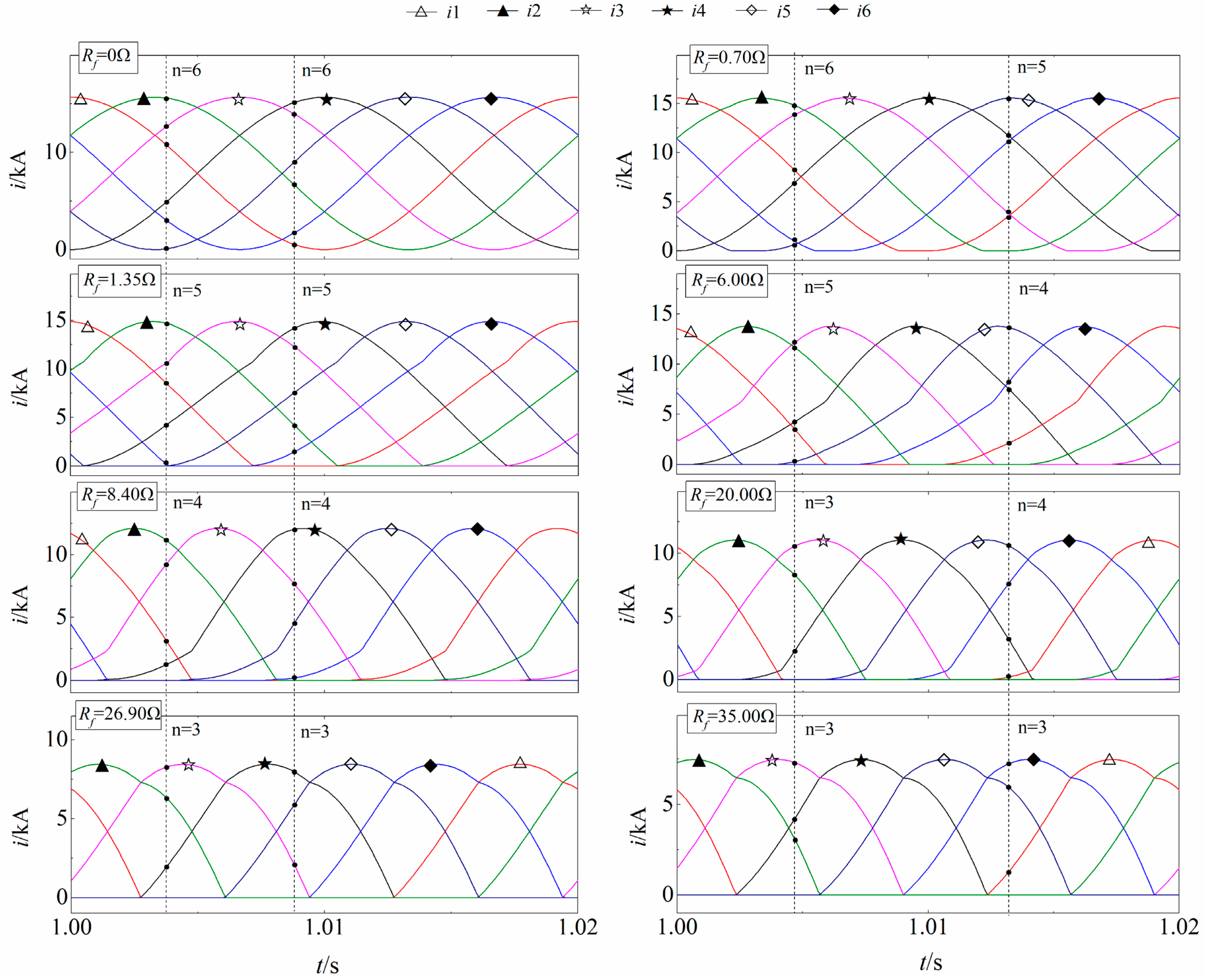
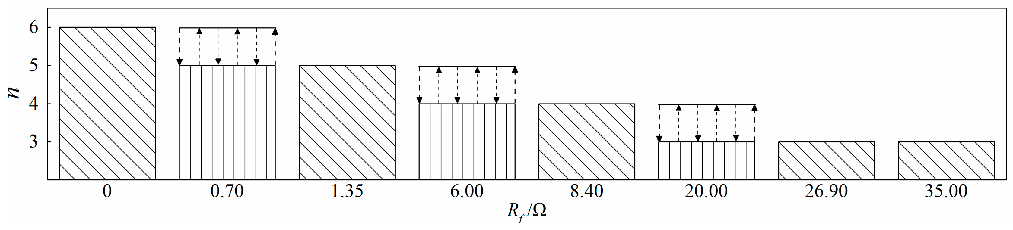
Fault resistance plays a significant role in suppressing the DC circulating current, thus influences the fault process. For a given MMC-HVDC system (detailed parameters are given in Appendix A Table A1 and the system is used to illustrate the analysis in the following sections), the simulation results of the arm currents under pole-to-pole faults with various fault resistances are shown in Figure 5. It is observed that the commutation overlapping phenomenon [22] of the arm current varies with fault resistance Rf. With increasing fault resistance, the DC circulating current decreases until it reaches zero; in such a process, the number of conducting diodes (NOCD) reduces. Classifying the NOCD in Figure 5, the relationship between NOCD and fault resistance is shown in Figure 6, and the following observations could be made:
- The NOCD decreases as the fault resistance rises.
- The NOCD remains constant when fault resistance is equal to certain values. Specific values of Rf are adopted here as 0/1.35/8.40/26.90 Ω for example. This could vary with different systems and will be discussed in Section 4.
- The NOCD alternately changes when the fault resistance is between the above certain values.
It should be noted that the NOCD is 2 when fault resistance is hundreds of ohms. However, the fault resistance rarely reaches such high values. Even if it does, the AC current under such fault resistance is extremely small. Therefore, this circumstance is not taken into consideration.
4. Simplified Analytic Approach of Pole-to-Pole Faults
In this section, a simplified analytical approach of pole-to-pole fault is proposed. First, critical resistance and critical state are defined to clarify the fault process. Then, critical states are analyzed including the determination of current loops and boundary conditions, and the derivation of fault current and critical resistance. The approximated expressions of fault current under arbitrary fault resistance are derived by linear combinations based on the critical states. In addition, the application of the expressions in the AC system backup protection setting calculation is recommended.
4.1. Definition of Critical Resistance and Critical State
According to Section 3, the NOCD varies with fault resistance, and may even alternately change when the fault resistance is between some specific values. This complicated characteristic of the fault process makes the derivation of fault current particularly challenging. To clarify the fault process, two definitions are given:
- Critical resistance: When the NOCD remains constant, the fault resistance is defined as critical resistance. Obviously, there are multiple critical resistances, and they are symbolized as Rc1, Rc2, Rc3, and Rc4, where the corresponding NOCD are 6, 5, 4, and 3, respectively.
- Critical state: The fault process under critical resistance is defined as the critical state, and the critical states are symbolized as c1, c2, c3, and c4, where the corresponding fault resistances are Rc1, Rc2, Rc3, and Rc4, respectively.
According to the definitions above, the fault process is in a critical state when the fault resistance is equal to the critical resistance; while it alternates between the two adjacent critical states when the fault resistance is between the corresponding two critical resistances. That is to say, the fault process under arbitrary fault resistance can be regarded as the combination of the adjacent critical states. Therefore, the analysis of fault process under arbitrary fault resistance can be simplified to the analysis of critical states.
4.2. Analysis of Critical States
In this part, the current loops and boundary conditions of critical state are determined as the basis for establishing the analytic equations. Then, the expressions of the fault current and critical resistances for the critical states are derived.
4.2.1. Determination of Current Loops
The current loops of c1, c2, c3, and c4 are shown in Figure 7. It shows that the DC circulating current, as the solid blue line, varied under different critical states. According to the characteristics of DC circulating current, c1, c2, c3, and c4 can be denoted as three-phase circulating state, two-phase circulating state, single-phase circulating state, and none-phase circulating state, respectively.
In any critical state, the conducting diodes in each period can be divided into six conducting sets. Each conducting set lasts for 60 degrees. For example, in the single-phase circulating state, the conducting sets are {D1,D2,D3,D4} -> {D2,D3,D4,D5} -> {D3,D4,D5,D6} -> {D4,D5,D6,D1} -> {D5,D6,D1,D2}-> {D6,D1,D2,D3} -> {D1,D2,D3,D4} in turn. Although the current loops of different conducting sets vary, the circuit equations in all the conducting sets are similar, as the rectifying process is periodic. Thus, the analysis can be based on one conducting set first, and then establishing the circuit equations. The expressions applicable for the whole period can be subsequently derived.
In the following analysis, the conducting sets {D1,D2,D3,D4,D5,D6}, {D1,D2,D3,D4,D5}, {D1,D2,D3,D4} and {D1,D2,D3} are selected for the three-phase, two-phase, single-phase, and none-phase circulating states, respectively. Their current loops are shown in Figure 7.
4.2.2. Determination of Boundary Conditions
The diodes turn on and off periodically in the critical states. Therefore, it can be drawn that the initial values of the diode conducting current in the present and the previous conducting sets are the same. For instance, in the single-phase circulating state, the initial value of i1 in {D1,D2,D3,D4} is the same as the initial value of i2 in {D2,D3,D4,D5}. The boundary conditions are expressed as follows:
where is the initial conducting angle.
In addition, it is well known that the diode follows the laws below: (1) turn on under forward voltage; and (2) turn off under reverse current. These laws are also chosen as the boundary conditions and expressed as follows:
where vn is the voltage of diodes Dn
4.2.3. Derivation of Fault Current and Critical Resistance
Since the current loops and boundary conditions were determined, the current differential equations of critical states are established in Equation (4) regardless of the fault inductance.
where A, B, and C are the coefficient matrices of differential current, arm current, and mid-arm voltage, respectively.
The boundary condition equations are:
where EmL−L is the line-to-line voltage of the mid-arm.
For instance, the current differential equations of the single-phase circulating state are as follows:
where:
The boundary condition equations are:
where is the line-to-line mid-arm voltage of phase A to phase C.
It is worth noting that Equations (4)–(6) do not involve the AC system parameters. However, the impact of the AC system on the fault process has already been taken into consideration, as it is reflected in the magnitude and phase of EmL−L. In addition, the boundary condition equations of three-phase circulating state are not included in Equation (5), as the diodes in this state always stay in conduction.
Combing Equations (4)–(6), and the critical resistance Rc and arm current in are yielded as:
Equation (13) indicates that the critical resistance Rc is related to the arm reactor Ls and demonstrates that the DC circulating current, which forms due to the existence of arm reactors, varies in different critical states.
The AC current iac is correlated with the arm current in. Figure 8 shows the comparison between AC current iac and arm current in, and the fundamental frequency harmonics component analysis of iac. It illustrates that: (1) the peak value and phase of iac and in are the same, regardless of whether the DC circulating current exists; and (2) the harmonic component of iac is negligible. Thus, the peak value and phase of fundamental frequency current are considered to be the same as the arm current in regardless of the harmonic component.
With the conclusion above, the fundamental frequency current can be obtained by the arm current in, and further simplified as Equation (15) (an example is listed in Appendix B).
where Req and Xeq are the equivalent resistance and reactance, respectively. α is the phase lag of iac to Em.
Since the mid-arm voltage Em is unknown while the AC source voltage E is already known, Equation (15) is rewritten as Equation (16). The equivalent circuit is shown in Figure 9, where Xt is the reactance of the transformer, and β is the phase lag of iac to E.
The RMS current is as follows:
In addition, the DC current is derived as follows:
where idc is the DC current. For instance, idc = i2 + i4 can be derived in the single-phase circulating state.
4.3. Analysis of Fault Process under Arbitrary Fault Resistance
The expressions of the fault current for critical states were derived in the previous section. As aforementioned, the fault process under arbitrary fault resistance can be regarded as a combination of adjacent critical states. The question of how to combine the two corresponding critical states when the fault resistance is between two adjacent critical resistances to obtain the expressions of fault current under arbitrary fault resistance is investigated in this section.
For any given fault resistance Rf, with the adjacent critical resistances of Rci and Rc(i+1), its corresponding expressions of fault current for adjacent critical states are Iac/dc_i(Rci) and Iac/dc_i+1(Rc(i+1)). Substituting Rf into Iac/dc_i(Rci) and Iac/dc_i+1(Rc(i+1)), the two calculation results Iac/dc_i(Rf) and Iac/dc_i+1(Rf) are obtained and drawn as squares in the resistance–current graph. The simulation results Iac/dc(Rf) under fault resistance Rf, are drawn as asterisks in the same graph and compared with the calculation results. Eight given fault resistances Rf (f = 1, …, 8) are selected and the comparison is shown in Figure 10. Iac/dc_(1,2,3,4)(Rf) is the fundamental frequency current or DC current calculation result obtained by the expressions for three-phase, two-phase, single-phase, and none-phase circulating states, respectively.
It is observed that: (1) When Rf = [Rci,Rc(i+1)], the simulation result is always within the calculation results obtained by the expressions for two adjacent critical states, that is, these two calculation results are the upper and lower limit of the simulation result, respectively. Moreover, the simulation results are close to the line that connected these two calculation results. (2) When Rf ≥ Rc4, the calculation result is almost the same as the simulation result, since the NOCD was always 3.
According to the above observation, the linear combination technique is employed to derive the approximate expressions of fault current for the fault process under arbitrary fault resistance, which is based on the expressions for critical states.
- Rf = [Rci,Rc(i+1)) (i = 1, 2, 3)
- Rf ≥ Rc4
To meet the requirements of the selectivity and sensitivity of AC system backup protections in all reasonable cases, the setting calculation is usually based on the most severe conditions. From the selectivity point of view, the most severe condition corresponds to the highest fault current under Rf = 0. This is the three-phase circulating state and the fault current can be calculated precisely. From the sensitivity point of view, the most severe condition corresponds to the lowest fault current under the largest Rf, when the fault occurs at the remote ends of the DC line. If the largest Rf is between two adjacent critical resistances, the expression of the critical state corresponding to the lower limit of the simulation result could be applied in the setting calculation. If a more precise result is needed, the approximated Equations (19) and (21) could be applied in the setting calculation.
5. Validations
5.1. MMC-HVDC System
To validate the feasibility of the proposed approach in different systems, it was applied in two MMC-HVDC systems, and the detailed parameters are given in Appendix A. Pole-to-pole faults in different locations were set in this system. The calculation results of the proposed approach were compared with those of the PSCAD/EMTDC simulations in the following.
5.2. Validations of the Proposed Approach
The results of the critical resistance are given in Table 1, which shows that the calculation results were similar to the simulation results, and the calculation errors were within 5%. With the critical resistances obtained, the fundamental frequency current Iac (RMS value) and DC current Idc were calculated and are given in Table 2. Compared to the simulation results, the errors of the calculation results were within 10%, while, in most of the conditions, the errors were below 5%.
The errors were mainly due to two factors: (1) the fault process had non-linear characteristics, so the method of linear combination resulted in a small amount of error; and (2) the harmonic component was ignored when calculating the fundamental frequency current.
The comparison of the calculated AC currents and simulated ones showed that the calculation errors of the fundamental current by the proposed approach were within 10%. The 10% error was acceptable, as the same level of measurement errors of the current transformer (CT) applied in protection measurements are regarded as acceptable in protection setting calculations [27]. To avoid relay overtripping or failure, the sensitivity factor could be modified according to the error level.
In addition, since the planning of MMC-HVDC projects requires many time-consuming transient simulations in general, the DC current calculated by the proposed approach could be employed as a fast preliminary calculation for the reference of planning MMC-HVDC projects.
6. Conclusions
This paper proposed a simplified analytic approach of pole-to-pole faults in MMC-HVDC for the AC system backup protection setting calculation. According to the standard AC system protection setting calculation, the principles of pole-to-pole faults analysis were investigated. The influence of fault resistance on pole-to-pole faults was discussed. Critical resistance and critical states were defined. The current loops and boundary conditions of critical states were determined, and the expressions of fault current under critical states were derived. The approximated expressions of fault current for the fault process under arbitrary fault resistance were derived by the method of linear combination. Finally, the proposed approach was verified by PSCAD/EMTDC simulations. The conclusions are as follows:
- The calculation errors of the fault current by the proposed approach were within 10%, which is acceptable for the AC system backup protection setting calculation. In addition, the proposed approach could provide a fast, preliminary calculation for the reference of planning MMC-HVDC projects.
- The arm reactor plays a significant role in the formation of the DC circulating current, and the fault process is influenced by the fault resistance. The concept of critical resistance and critical state were defined, and the fault process can be regarded as a combination of critical states.
- The expressions of fault current for critical states, and the approximated expressions of fault current for fault processes under arbitrary fault resistance were derived. When the fault resistance is between two adjacent critical resistances, the results calculated by the expressions for corresponding critical states are the upper and lower limits of the simulation results.
- For the faults with arbitrary fault resistance, the expressions of fault currents for the adjacent critical states could be applied in the AC system backup protection settings calculation, depending on requirements of selectivity or sensitivity. If a more precise result is needed, the approximated expressions, a linear combination of the expressions for the critical states, could be applied in the setting calculation.
- The simplified analytic approach of pole-to-pole faults in two-level and three-level VSC-HVDCs for AC system backup protection will be investigated in our future work, since the two-level and three-level VSCs are also not capable of clearing the pole-to-pole fault by blocking the converter.
Acknowledgments
The authors have gratefully acknowledged the State Key Laboratory of Advanced Electromagnetic Engineering and Technology, Hubei Electric Power Security and High Efficiency Key Laboratory, School of Electrical and Electronic Engineering and Huazhong University of Science and Technology for providing necessary facilities.
Author Contributions
All authors have contributed to this research work. Tongkun Lan, Yinhong Li and Xianzhong Duan developed the research framework. Tongkun Lan, Yinhong Li and Jia Zhu performed the simulations, discussed the analyzed and wrote the manuscript. Xianzhong Duan suggested the research idea and reviewed the manuscript.
Conflicts of Interest
The authors declare no conflict of interest.
Appendix A

Table A1.
Parameters of MMC-HVDC system #1.
| Parameters | Values | Parameters | Values |
|---|---|---|---|
| AC System Line-to-Line Voltage/kV | 370 | DC Bus Voltage/kV | ±320 |
| Transformer Inductance/mH | 25.4 | Active Power/MW | 1000 |
| Arm Reactor/mH | 30 | Reactive Power/MVar | 0 |
| DC Line Resistance Ω/km | 0.0139 | Numbers of Sub-module | 152 |
| DC Line Inductance mH/km | 0.159 | Sub-module Capacitor/μF | 2800 |
Table A2.
Parameters of MMC-HVDC system #2.
| Parameters | Values | Parameters | Values |
|---|---|---|---|
| AC System Line-to-Line Voltage/kV | 370 | DC Bus Voltage/kV | ±320 |
| Transformer Inductance/mH | 36.3 | Active Power/MW | 1000 |
| Arm Reactor/mH | 50 | Reactive Power/MVar | 0 |
| DC Line Resistance Ω/km | 0.0139 | Numbers of Sub-module | 152 |
| DC Line Inductance mH/km | 0.159 | Sub-module Capacitor/μF | 2800 |
Appendix B
Fault current calculation, single-phase circulating state.
Solving Equation (7), the general solution of i1–i4 are as follows:
where C1, C2, and C3 are constants; is the conducting angle; and .
Combining the boundary conditions (Equations (11) and (12)), the critical resistance is yielded. The special solutions of i1–i4 are also obtained. In the conducting set {D1,D2,D3,D4}, current i2 has reached its peak value. Thus, the peak value and phase of iac is obtained, and is rewritten to form Equation (15).
It is assumed that El−l = 370 kV, Ls = 30 mH, Lt = 25.4 mH, and Rl = Rc3. The mid-arm voltage is set to . The results are as follows (phase A):
The fundamental frequency current (RMS) and DC current are:
References
- Li, S.H.; Naoto, Y.; Ding, M.; Zoka, Y. Sensitivity analysis to operation margin of zone 3 impedance relays with bus power and shunt susceptance. IEEE Trans. Power Deliv. 2008, 23, 102–108. [Google Scholar] [CrossRef]
- Garlapati, S.; Lin, H.; Heiber, A.; Shukla, S.K.; Thorp, J. A hierarchically distributed non-intrusive agent aided distance relaying protection scheme to supervise zone 3. Electr. Power Energy Syst. 2013, 42–49. [Google Scholar] [CrossRef]
- Zhong, Y.; Kang, X.N.; Jiao, Z.B.; Wang, Z.C.; Suonan, J.L. A novel distance protection algorithm for the phase-ground fault. IEEE Trans. Power. Deliv. 2014, 29, 1718–1725. [Google Scholar] [CrossRef]
- Saumendra, S.; Ashok, K.P. Synchronised data-based adaptive backup protection for series compensated line. IET Gener. Transm. Distrib. 2014, 8, 1979–1986. [Google Scholar]
- Ma, J.; Xiang, X.Q.; Kang, W.B.; Thorp, J.S. A novel algorithm of regional backup protection using adaptive current protection suiting factor. Int. Trans. Electr. Energy Syst. 2017, 27, 2399. [Google Scholar] [CrossRef]
- Denholm, P.; Margolis, R.; Mai, T.; Brinkman, G.; Drury, E.; Hand, M.; Mowers, M. Bright future: Solar power as a major contributor to the U.S. grid. IEEE Power Energy Mag. 2013, 11, 22–32. [Google Scholar] [CrossRef]
- Máslo, K.; Pestana, R.; Strunz, K.; Moroni, S.; Centeno, P. Innovative grid and generation technologies for future European power system. In Proceedings of the 12th International Conference on the European Energy Market (EEM), Lisbon, Portugal, 19–22 May 2015; pp. 1–5. [Google Scholar]
- Xu, Z.; Dong, H.F.; Huang, H.Y. Debates on ultra-high-voltages synchronous power grids: The future super grid in China? IET Gener. Transm. Distrib. 2015, 9, 740–747. [Google Scholar] [CrossRef]
- Lesnicar, A.; Marquardt, R. An innovative modular multilevel converter topology suitable for a wide power range. In Proceedings of the IEEE Bologna Powertech Conference, Bologna, Italy, 23–26 June 2003; pp. 1–6. [Google Scholar]
- Marquardt, R. Modular Multilevel Converter: An universal concept for HVDC-Networks and extended DC-Bus Applications. In Proceedings of the IEEE ECCE-Asia IPEC 2010, Sapporo, Japan, 21–24 June 2010. [Google Scholar]
- Suman, D.; Qin, J.C.; Behrooz, B.; Maryam, S.; Peter, B. Operation, control, and applications of the modular multilevel converter: A review. IEEE Trans. Power Deliv. 2015, 30, 37–53. [Google Scholar]
- Ding, H.; Wu, Y.K.; Zhang, Y.; Ma, Y.L.; Kuffel, R. System stability analysis of Xiamen bipolar MMC-HVDC project. In Proceedings of the 12th IET International Conference on AC and DC Power Transmission, Beijing, China, 28–29 May 2016; pp. 1–6. [Google Scholar]
- Buigues, G.; Valverde, V.; Etxegarai, A.; Eguía, P.; Torres, E. Present and future multi-terminal HVDC systems: Current status and forthcoming developments. In Proceedings of the International Conference on Renewable Energies and Power Quality, Malaga, Spain, 4–6 April 2017; pp. 83–88. [Google Scholar]
- Tang, L.X.; Ooi, B.-T. Locating and isolating DC faults in multi-terminal DC systems. IEEE Trans. Power Deliv. 2007, 22, 1877–1884. [Google Scholar] [CrossRef]
- Zhang, J.P.; Zhao, C.Y. The research of SM topology with DC fault tolerance in MMC-HVDC. IEEE Trans. Power Deliv. 2015, 30, 1561–1568. [Google Scholar] [CrossRef]
- Yang, J.; Fletcher, J.E.; O’Reilly, J. Multiterminal DC wind farm collection grid internal fault analysis and protection design. IEEE Trans. Power. Deliv. 2010, 25, 2308–2318. [Google Scholar] [CrossRef]
- Flourentzou, N.; Agelidis, V.G.; Demetrades, G.D. VSC-Based HVDC power transmission systems: An overview. IEEE Trans. Power Electron. 2009, 24, 592–602. [Google Scholar] [CrossRef]
- Xu, J.Z.; Zhao, C.Y.; Liu, W.J.; Guo, C.Y. Accelerated model of modular multilevel converters in PSCAD/EMTDC. IEEE Trans. Power Deliv. 2013, 28, 129–136. [Google Scholar] [CrossRef]
- Xu, J.Z.; Fan, S.T.; Zhao, C.Y.; Gole, A.M. High-speed EMT modeling of MMCs with arbitrary multi-port sub-module structures using generalized Norton equivalents. IEEE Trans. Power Deliv. 2017. [Google Scholar] [CrossRef]
- Khan, S.S.; Tedeschi, E. Modeling of MMC for fast and accurate simulation of electromagnetic transients: A review. Energies 2017, 10, 1161. [Google Scholar] [CrossRef]
- Bucher, M.K.; Frank, C.M. Analytic approximation of fault current contribution from AC networks to MTDC networks during pole-to-ground faults. IEEE Trans. Power Deliv. 2016, 31, 20–27. [Google Scholar] [CrossRef]
- Li, B.; He, J.W.; Tian, J.; Feng, Y.D.; Dong, Y.L. DC faults analysis for modular multilevel converter-based system. J. Mod. Power Syst. Clean Energy 2017, 5, 275–282. [Google Scholar] [CrossRef]
- Li, C.Y.; Zhao, C.Y.; Xu, J.Z.; Ji, Y.K.; Zhang, F.; An, T. A pole-to-pole short-circuit fault current calculation method for DC grids. IEEE Trans. Power Syst. 2017. [CrossRef]
- He, L.N.; Liu, C.C.; Pitto, A.; Cirio, D. Distance protection of AC grid with HVDC-connected offshore wind generators. IEEE Trans. Power Deliv. 2014, 29, 493–501. [Google Scholar] [CrossRef]
- Liu, Y.C.; Li, G.Q.; Wang, Z.H.; Yu, W.X. Research on AC line distance relay in the presence of modular multilevel converter based HVDC. In Proceedings of the IEEE PES Asia-Pacific Power and Energy Conference, Xi’an, China, 25–28 October 2016. [Google Scholar]
- Setting Guide for 220 kV~750 kV Power System Protection Equipment. Available online: http://www.gbstandards.org/index/GB_standard.asp?id=64137 (accessed on 18 October 2017).
- Bhalja, B.; Maheshwari, R.P.; Chothani, N. Protection and Switchgear, 1st ed.; Oxford University Press: New Delhi, India, 2011; pp. 169–201. ISBN 0198075502. [Google Scholar]
Figure 1.
Schematic diagram of pole-to-pole faults in MMC-HVDC (multi-modular converter based high voltage direct current).
Figure 1.
Schematic diagram of pole-to-pole faults in MMC-HVDC (multi-modular converter based high voltage direct current).

Figure 2.
Equivalent diagram of blocked MMC (multi-modular converter).

Figure 3.
AC current under pole-to-pole faults.
Figure 4.
Schematic diagram of DC circulating current.
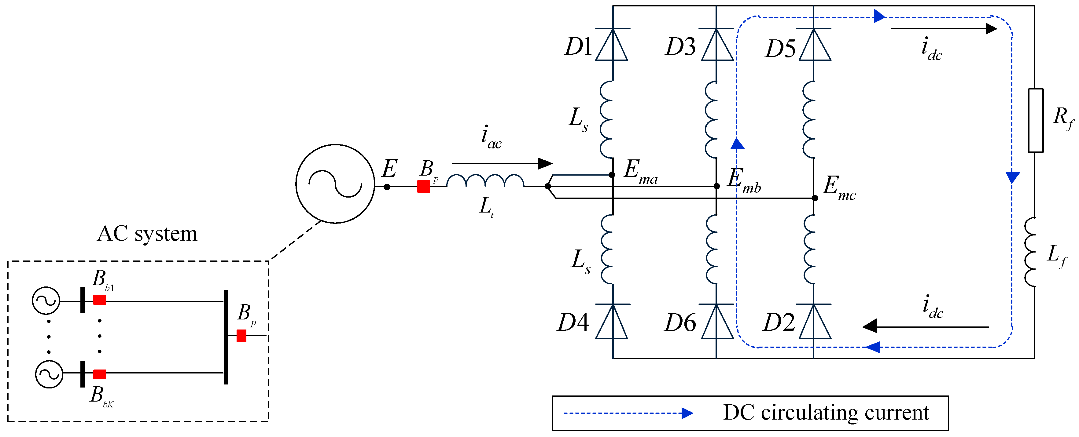
Figure 5.
Arm current under pole-to-pole faults with variant fault resistance.

Figure 6.
Relationship between fault resistance and NOCD (number of conducting diodes).

Figure 7.
Current loops of critical states.

Figure 8.
Relationship between the AC current and arm current. (a) Exist circulating current; (b) No circulating current.
Figure 8.
Relationship between the AC current and arm current. (a) Exist circulating current; (b) No circulating current.

Figure 9.
Equivalent circuit and vector diagram. (a) Equivalent circuit; (b) Vector.
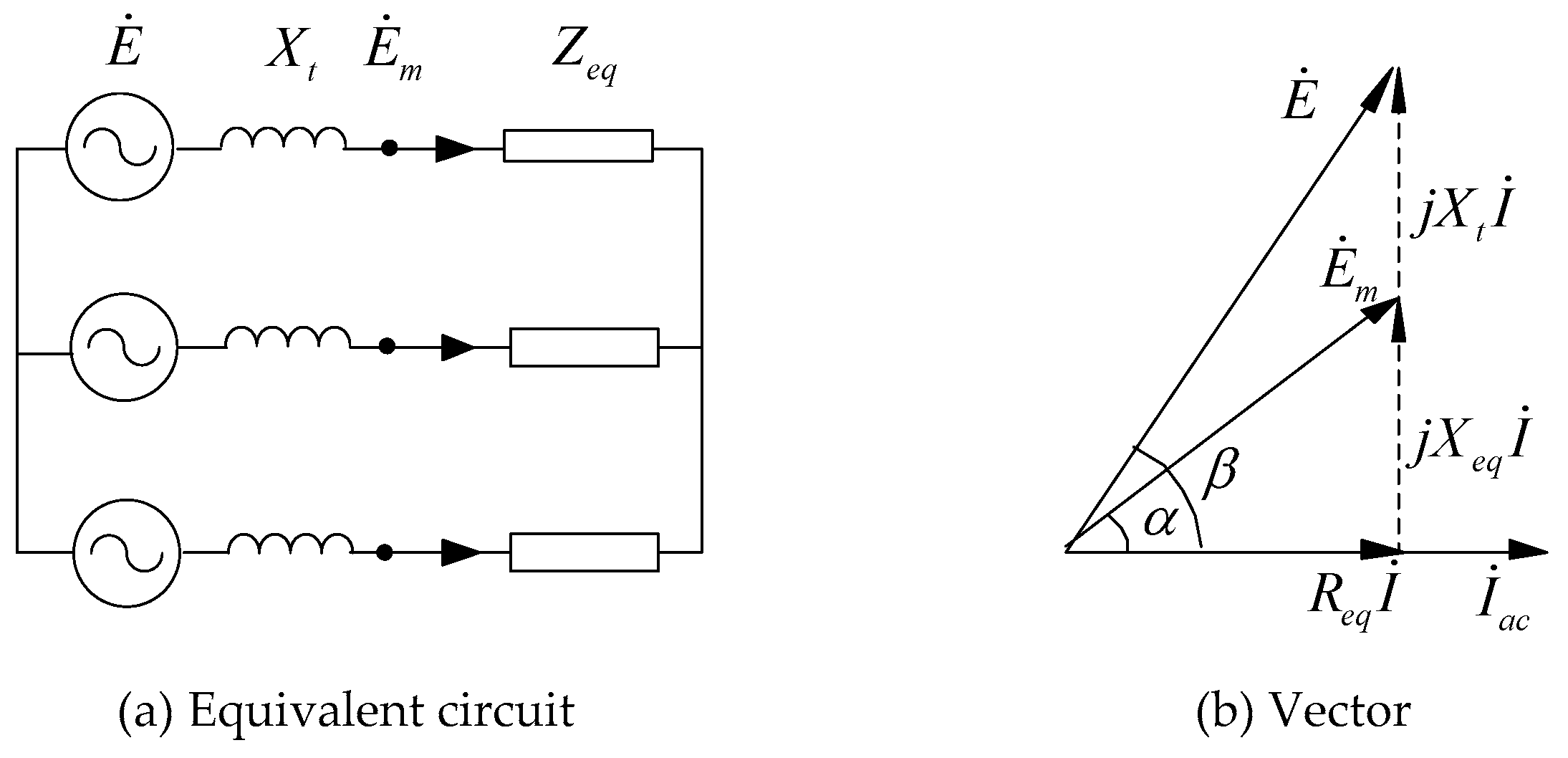
Figure 10.
Comparison between the simulation results and calculation results.

Table 1.
Comparison between calculation results and simulation results of critical resistance.
| Critical Resistance | Ls = 30 mH | Ls = 50 mH | ||||
|---|---|---|---|---|---|---|
| Calculation | Simulation | Error | Calculation | Simulation | Error | |
| Rc1/Ω | 0 | 0 | 0 | 0 | 0 | 0 |
| Rc2/Ω | 0.77 | 0.80 | −3.8% | 1.29 | 1.35 | −4.4% |
| Rc3/Ω | 4.96 | 5.05 | −1.8% | 8.27 | 8.40 | −1.5% |
| Rc4/Ω | 16.32 | 16.15 | 1.1% | 27.20 | 26.90 | 1.1% |
Table 2.
Comparison between the calculation results and simulation results of fault current.
| Inductance/mH | Fault Resistance/Ω | Iac/kA | Idc/kA | |||||
|---|---|---|---|---|---|---|---|---|
| Lt | Ls | Calculation | Simulation | Error | Calculation | Simulation | Error | |
| 25.4 | 30 | 0.00 | 16.84 | 16.83 | 0.1% | 35.72 | 35.69 | 0.1% |
| 0.50 | 16.29 | 16.48 | −1.2% | 33.14 | 31.91 | 3.9% | ||
| 0.77 | 16.03 | 16.25 | −1.4% | 31.38 | 30.46 | 3.0% | ||
| 3.00 | 15.24 | 14.45 | 5.5% | 24.44 | 22.82 | 7.1% | ||
| 4.96 | 13.76 | 13.28 | 3.6% | 20.57 | 19.16 | 7.4% | ||
| 10.00 | 11.51 | 11.66 | −1.3% | 16.27 | 15.95 | 2.0% | ||
| 16.32 | 10.41 | 10.17 | 2.4% | 14.03 | 13.70 | 2.4% | ||
| 25.00 | 8.87 | 8.59 | 3.3% | 11.95 | 11.50 | 3.9% | ||
| 36.3 | 50 | 0.00 | 11.09 | 11.08 | 0.1% | 23.54 | 23.53 | 0.1% |
| 0.70 | 10.76 | 10.89 | −1.2% | 22.00 | 21.31 | 3.2% | ||
| 1.29 | 10.51 | 10.67 | −1.5% | 20.59 | 19.99 | 3.0% | ||
| 6.00 | 9.67 | 9.10 | 6.3% | 15.24 | 13.95 | 9.2% | ||
| 8.27 | 8.89 | 8.55 | 4.0% | 13.29 | 12.34 | 7.7% | ||
| 20.00 | 6.99 | 7.07 | −1.1% | 9.81 | 9.61 | 2.1% | ||
| 27.20 | 6.55 | 6.40 | 2.3% | 8.84 | 8.62 | 2.6% | ||
| 35.00 | 5.97 | 5.79 | 3.1% | 8.06 | 7.76 | 3.9% | ||
© 2018 by the authors. Licensee MDPI, Basel, Switzerland. This article is an open access article distributed under the terms and conditions of the Creative Commons Attribution (CC BY) license (http://creativecommons.org/licenses/by/4.0/).
Share and Cite
MDPI and ACS Style
Lan, T.; Li, Y.; Duan, X.; Zhu, J. Simplified Analytic Approach of Pole-to-Pole Faults in MMC-HVDC for AC System Backup Protection Setting Calculation. Energies 2018, 11, 264. https://doi.org/10.3390/en11020264
AMA Style
Lan T, Li Y, Duan X, Zhu J. Simplified Analytic Approach of Pole-to-Pole Faults in MMC-HVDC for AC System Backup Protection Setting Calculation. Energies. 2018; 11(2):264. https://doi.org/10.3390/en11020264
Chicago/Turabian StyleLan, Tongkun, Yinhong Li, Xianzhong Duan, and Jia Zhu. 2018. "Simplified Analytic Approach of Pole-to-Pole Faults in MMC-HVDC for AC System Backup Protection Setting Calculation" Energies 11, no. 2: 264. https://doi.org/10.3390/en11020264
Note that from the first issue of 2016, this journal uses article numbers instead of page numbers. See further details here.