District Heating Expansion Potential with Low-Temperature and End-Use Heat Savings


1
Department of Development and Planning, Aalborg University, Rendsburggade 14, DK-9000 Aalborg, Denmark
2
Department of Development and Planning, Aalborg University, A. C. Meyers Vænge 15, DK-2450 København SV, Denmark
*
Author to whom correspondence should be addressed.
Energies 2018, 11(2), 277; https://doi.org/10.3390/en11020277
Submission received: 12 December 2017
/
Revised: 13 January 2018
/
Accepted: 15 January 2018
/
Published: 24 January 2018
Abstract
:District heating has the potential to play a key role in the transition towards a renewable energy system. However, the development towards reduced heat demands threatens the feasibility of district heating. Despite this challenge, opportunity exists in the form of fourth generation district heating, which operates at lower temperatures and enables better renewable integration. This article investigates this challenge by examining the district heating potential within three scenarios: The first is a reference scenario with current heat demand and temperatures, the second includes heat demand savings and the third includes reduced grid temperatures in addition to heat savings. To examine the scenarios, two models are developed. The first is a heat atlas model, in which heat demands are mapped on an address level. The second model assesses district heating expansion potentials based on economic costs. The models are applied using an example case of The Northern Region of Denmark. The article concludes that the district heating potential is highest in the reference scenario. When heat savings are introduced, district heating expansions, in most cases, will not be feasible. Introducing low-temperature district heating modestly increases the feasible expansion potential. This general conclusion is highly dependent on the specific system examined.
1. Introduction
An increased focus on large-scale renewable energy integration promotes the concept of smart energy systems [1]. Smart energy systems focus on the integration of all energy sectors-electricity, heating, industries, and transport-and call for high flexibility in both production and consumption. The flexibility and integration of energy sectors are needed to integrate large shares of fluctuating renewable energy. In these smart energy systems, district heating is a key technology for integrating the heat and electricity sectors in dense urban areas. District heating has several benefits related to the integration of renewable energy sources. One benefit is its large heat storage capacity [2], which can store much more heat than individual storage solutions. Another benefit is the ability to utilize heat from a variety of sources, such as solar thermal, geothermal, and excess production from industrial processes as well as heat from combined heat and power plants [3,4,5,6]. A recent Chinse study shows the benefits of combing the heat and electricity sectors in terms of wind curtailment [7]. On the other hand, there are also disadvantages to the technology, and thus district heating needs to change to be relevant in a smart energy system with a large share of renewable energy. One disadvantage is the heat losses in the distribution grids, which are between 8–35% in European systems [8]. These losses are most significant when supplying areas with low heat density, but can also be attributed to the high temperature level in current systems, which have a typical forward temperature of around 80 °C. The heat distribution loss is important because most future scenarios implement large heat savings in existing buildings [9,10], while the requirements for new buildings are approaching near zero energy standards [11,12], resulting in a relatively higher share of network losses in the future if the same system properties are kept. Moreover, the temperature level is important because it hinders an efficient implementation of some renewable energy technologies that only supply heat at much lower temperatures, such as geothermal and solar thermal energy, or technologies like large-scale heat pumps [13] that benefit from lower supply temperatures. Therefore, considerable research efforts are being spent investigating the next generation of district heating, the so-called fourth generation [14]. The characteristics of fourth generation district heating are that the system temperatures are lower and a large variety of supply sources, mainly based on renewable energies, can be included. Much of the research examines new district heating concepts, with considerable focus given to the application of different system temperature levels, including low-temperature (55 °C) and even ultra-low temperature (35 °C) [15,16]. These studies conclude that switching to ultra-low temperature reduces the grid losses but adds to the general system costs, and is therefore not an attractive solution. Thus, the best option for most systems seems to be low-temperature district heating.
The potential for low-temperature district heating has primarily been assessed in energy systems analysis models, which show the synergies of the technology with the potential energy supply in renewable energy scenarios. However, an important aspect of district heating is the investment cost of the heating networks. The investment costs of district heating networks relate to the geographic placement of the buildings and associated heat demands. The closer the buildings are situated, the smaller the network need be, thereby reducing investment costs. Thus, a mapping of heat demands is required to determine if a location is suitable for district heating. Typically, the mapping of heat demands is done in a heat atlas for the location in question. Heat atlases come in all shapes and forms and are used for various purposes. Some are used to illustrate the geographic location of heat demands, with some recent examples including Paris [17] and London [18]. Others use heat atlases to estimate heat demands in energy strategies for cities or communities [19,20,21,22], countries [23,24] or even on a European level [25,26]. Recently, the authors of this article have used heat atlases to develop inputs for the planning of district heating expansions [27,28,29,30]. The primary aim of these plans is to serve as inputs for local policymakers and utilities when making decisions on new heating infrastructure. The heat atlas used for these plans is called The Danish Heat Atlas and includes all buildings in Denmark. The Danish Heat Atlas exists in several versions, in which the heat demand models have been developed and improved over time [31,32]. Since 2010, Danish legislation requires all suppliers of oil, natural gas, and district heating to send information regarding annual energy consumption to a central database named FIE, which is a Danish abbreviation for The Supply Companies Reporting Model for Energy Consumption. At present, the FIE database includes around half of all Danish buildings. This provides a quite comprehensive dataset, and offers the ability to improve the heat consumption models for Danish buildings that have been used to establish previous heat atlases [33].
2. Aim of the Article
The aim of this article is twofold: The first part is to analyse the registered heat demands of buildings from the FIE database and to create a heat atlas based on these demands. The second part is to show the application of the heat atlas by assessing the district heating potential in a specific case. The case used is the northern region of Denmark, which consists of around 368 thousand buildings, of which 153 thousand already have district heating. The expansion potential of district heating in this case will be analysed with both standard and low-temperature district heating options. This is done to examine the challenges arising if the considerable renovations to the building stock included in many long-term energy plans are realised.
3. Methodology
This section describes the methodologies used in the article. The first part details the development of the heat atlas, while the second presents the district heating expansion model.
3.1. Development of a New Heat Atlas
In Denmark, the primary data source on buildings is the national building register. The register includes most building properties and covers all buildings in Denmark. The register is a central register but is updated through a bottom-up approach, where the responsibility to update the information is placed upon individual building owners. The register includes information on the size, type, age and energy supply type of each building. However, prior to 2010, the building register did not include information about the energy demand of buildings. Since 2010, energy demand data has been collected in the FIE database. The FIE data currently come from district heating, natural gas, and oil suppliers, and will also include electricity demands in future versions. Due to the way energy is registered, the FIE database cannot include all of Denmark’s heated buildings. It is estimated that when the database is fully implemented, it will cover around 80% of the heated buildings in Denmark [34].
As the FIE data is updated on a continuous basis, the data will vary depending on which version is used. The version used in this article is from July 2016 and includes 5.27 million measurements. Table 1 shows an overview of the data.
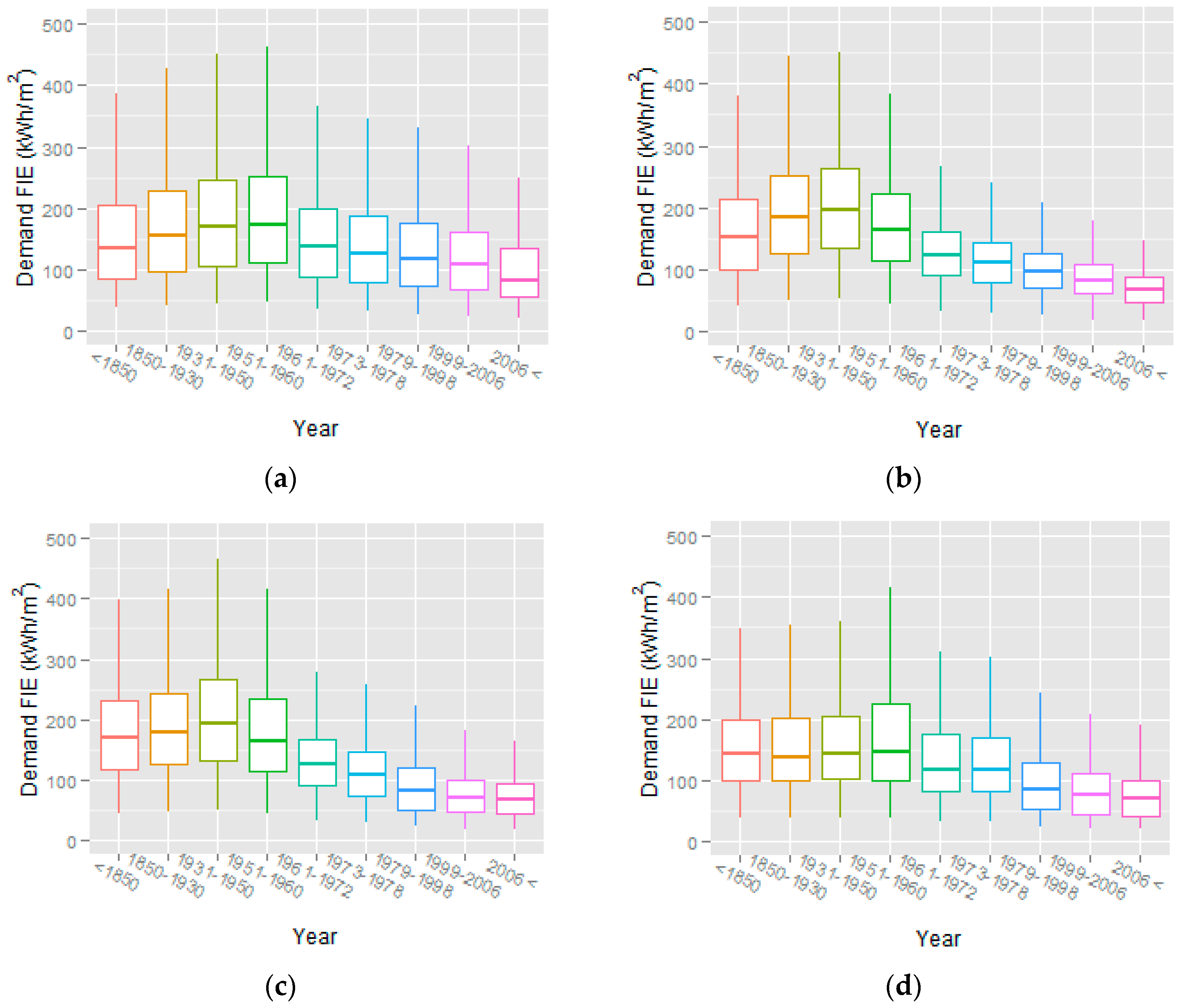
As seen in Table 2, the category with the most measurements is the residential sector. Thus, the subcategories within the residential sector are used as exemplary cases on how the heat demand is estimated in the Danish Heat Atlas. In the heat atlas, a total of 32 building categories are included, but these will not be presented in this article due to space limitations. The subcategories of the residential sector were analysed using the statistical computing software R and the results are shown as boxplots in Figure 1. The outliers have been excluded since the high number of input data points results in many outliers, making it difficult to identify individual outliers. However, it is important to note that there are significant outliers, as the heat consumption in individual buildings can be 8–10 times more than the average for the category. This means that the uncertainty of the analysis is higher in areas with few buildings, as one outlier within these areas has a high impact on the total heat demand. Having said that, as heat demand density is an important factor for determining the economic feasibility of district heating, areas with very few buildings are unlikely to present good business cases for district heating, and this uncertainty therefore has a relatively small impact on the overall analysis.
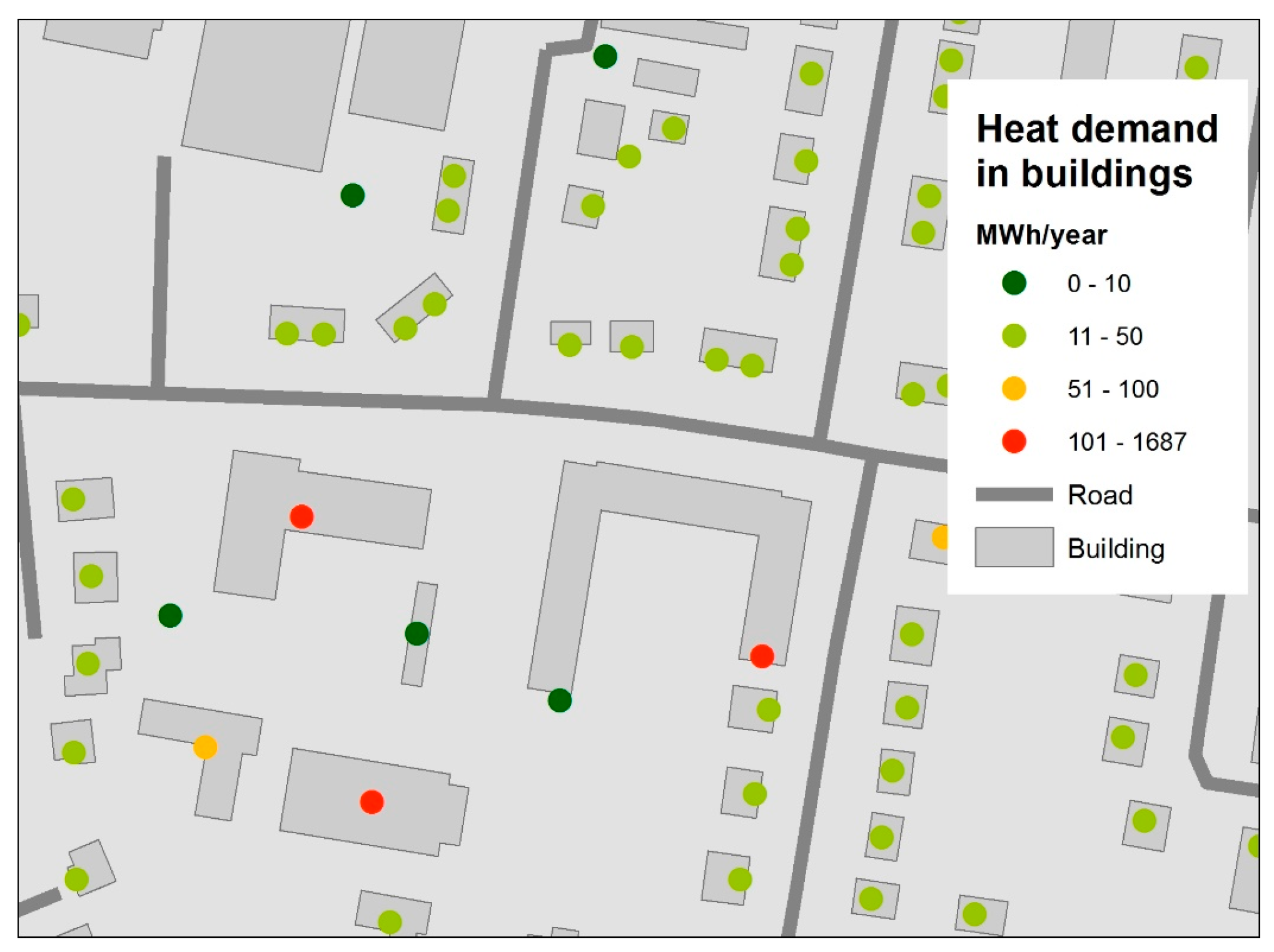
Each of the four box plots represents a different building category; the x-axis shows typical construction periods and the y-axis shows the demand per m2 floor area for each building type. Furthermore, the values are shown as percentiles, showing the spread of values for each category. As expected, the spread is quite large within all categories, which is due to variation in building use, inhabitants and simply the difference in the building stock. It is also clear that buildings from 1951–1972 typically have high demands, whereas buildings built before 1951 and from 1972–1999 have lower demands. The lowest demands are found in buildings erected after 1999, likely due to the higher requirements in buildings construction codes. In the heat atlas, the mean value in kWh/m2 is used to estimate the demand for each building type and construction period. Figure 2 shows the output of this method; it is clear that the heat demand follows the size of the building, with larger buildings typically having higher demands.
To sum up, the heat atlas is generated by using the statistical values for average heat consumption in buildings according to the time period and building type calculated from the FIE data. These values are used to calculate an estimated heat demand for all Danish buildings using the building values from the national building register, including the spatial location of each building.
3.2. Scenarios for District Heating Expansion Potential
To demonstrate the applicability of the developed heat atlas, it is used to examine the district heating expansion potential in a specific area of Denmark. As the expansion potential has been examined under current conditions of heat demand and temperature levels in previous articles [27,29,30], we include cases with significant heat savings as well as low-temperature district heating. Thus, the following three scenarios are analysed:
- Standard district heating
- Standard district heating with heat savings
- Low-temperature district heating with heat savings
The first scenario is the reference case, which reflects the existing situation with current heat demands and current supply/return temperatures of 80/40 °C. The second scenario considers the same temperature levels but includes 50% heat savings in the space heat demand of the buildings. The third scenario includes the same heat savings as scenario two, but also implements low-temperature district heating at supply/return temperatures of 55/25 °C. The justification for these three scenarios is as follows: The first scenario is expected to have a high district heating potential, as this scenario has the highest heat densities. However, as most long-term energy plans include end-use heat savings, the district heating potential should also be evaluated in this long-term context, hence the inclusion of the second scenario. It is expected that end-use heat savings reduces the heat densities and thus the district heating expansion potential. On the other hand, end-user savings also enable a shift towards low-temperature district heating, which will lower the heat losses. Scenario three examines how this change to low-temperature will affect the district heating expansion potential. According to [35], the presence of over-dimensioned radiators in combination with general renovations and higher internal heat gains from electrical appliances makes it possible to heat the existing Danish building stock using lower temperatures.
3.3. The District Heating Expansion Model
The model description consists of price and cost inputs as well as the method or procedure used in the model.
3.3.1. Prices and Cost Inputs
A GIS (Geographical Information System) model is developed in order to examine the expansion potential of district heating. The GIS model aims to be able to make a screening of the district heating expansion potential based on economic costs. Often, the perspective in economic analyses of district heating potentials is made from either an investor or societal point of view. However, in this example, the consumer costs will be the economic indicator used to examine the district heating potential. The rationale for using consumer costs is that if the expansion is not feasible for the consumers, they cannot be expected to change to district heating. As with the heat densities in a potential district heating area, the heat price has a huge impact on the feasibility of district heating expansion. Therefore, if expansion is not feasible based on current heat prices, the supply company should try to reduce heat prices before expanding further. Thus, the model can also be used to look at the competitive situation of heat prices in each district heating area, and not only the district heating expansion potential.
The heat prices used in the model are from December 2016 [36] and are shown in Figure 3. From the figure, it is clear that the prices vary among the 422 district heating areas in Denmark, from around 20 €/MWh to 120 €/MWh. This variation is mainly due to differences in heat supply and population density within each district heating area. In general, areas with a high density of buildings are better suited for district heating, and given access to inexpensive heat sources, such as excess heat from industries, electricity production, and waste incineration, the heat prices can be reduced significantly. The access to inexpensive heat sources even allows district heating to be feasible in areas with lower population density. Low density areas are however vulnerable to price changes, compared to areas with higher densities. A Danish study [37] of price differences made in 2012, concluded that what influences the prices in a district heating area is the primary fuel type used, the ownership of the system as well as scale of the system. However, the analysis also concludes that other factors should be analysed such as the size of the grids, consumer density, depreciation as well as age of the systems.
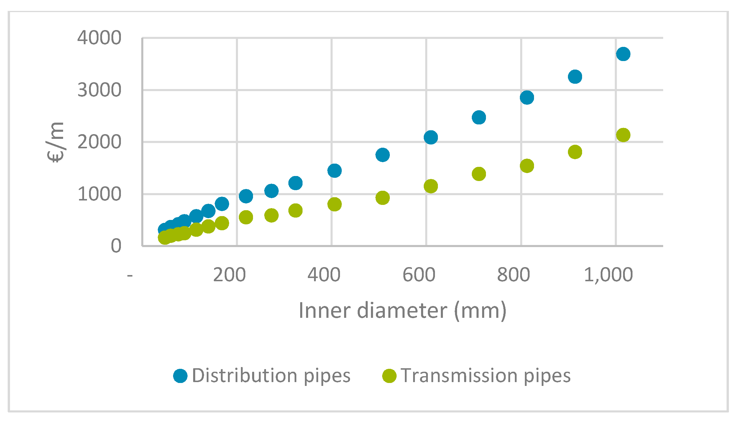
Besides heating prices, the investment costs of the heat network are important. In the GIS model, these costs are divided into distribution and transmission grids. This is primarily due to a difference in the costs of burying pipes within urban and non-urban areas. It is assumed that the distribution grids within urban areas have higher excavating costs than transmission lines, which are located outside urban areas. The costs are shown in Figure 4 and vary depending on the pipe diameter. Besides the costs for materials and digging, the investment price also includes project management, field work and pipework.
The final cost inputs for the district heating expansion model include the investment costs for installing service pipes and substations. These are assumed to be between 4500 and 7500 € per building, depending on its heat demand [39]. The model assumes that all investment costs related to district heating expansion are paid by the system’s new consumers. The heating price is assumed to include the amount needed to recover the investment cost of the existing network. This approach ensures that existing consumers are not negatively affected by the expansion of district heating networks. It is assumed that the existing heat generation facilities in the current district heating areas have sufficient capacity to supply the heat needed in the expanded grids. Further investigation into the production of heat for the expanded systems is therefore out of the scope of this paper, although it is acknowledged that changes to the heat generation facilities could affect the expansion feasibility, both positively and negatively.
3.3.2. Description of the GIS Model
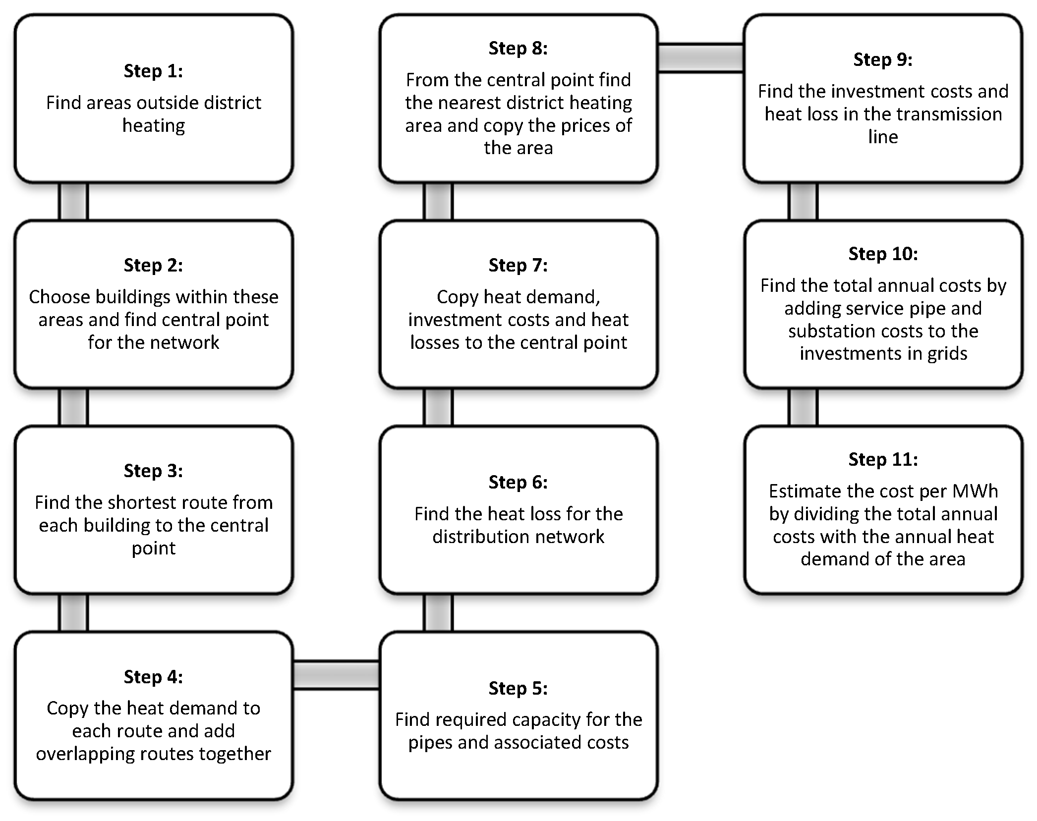
The GIS model consists of several Python scripts written for ESRI’s (Environmental Systems Research Institute) ArcMap software. The model attempts to estimate the heat price within towns that are not currently connected to district heating networks. Typically, this is done by manually determining the costs of building a new district heating network and connecting it to an existing area. The manual approach is highly labour intensive if carried out on a large scale, and thus, in the initial phase, a more automated process is useful to identify potential areas that warrant further analysis. This is where a screening tool, such as the one presented here, becomes relevant. However, it is important to remember that the final cost estimation still requires a more thorough approach, including a detailed dimensioning of the potential district heating network. Figure 5 shows the steps used to estimate the costs in the GIS model; these will be used in the following explanation of the model.
In Step 1, the potential areas that should be included in the analysis are found. In this article, the areas used are the towns that are not currently within existing district heating areas. The areas vary in size from two to 1345 buildings, which means that very small areas are also included. In total, 1001 areas were included in the analysis. In Step 2, the heat atlas is used to identify buildings and heat demands within each area. Additionally, the point towards which the distribution pipes should be directed is found. This is done automatically by selecting the geographical central point of each area. In principle, using the central point offers the lowest network cost, as it minimizes the distance to all buildings, but it might not be feasible in practice due to planning restrictions in the area. Step 3 follows existing roads to find the shortest route between all buildings and the central point in each area. This approach determines a distribution route for each building with an associated heat demand. In Step 4, the heat demand for all overlapping routes are added together to give the total heat that needs to be transferred through a given route. The total heat demand for all routes is used, in Step 5, to find the capacity of the grids as well as the associated investment costs. The required capacities vary depending on the temperature level in the grid; the capacities used for different pipe sizes are shown in Table 3.
Based on the above steps, a heat distribution network for each area is created, an example of which is illustrated in Figure 6. As shown, pipe sizes decrease as they get closer to the individual buildings in which the heat is used.
In Step 6, the annual heat loss is estimated for each area; this is based on a heat loss per meter of pipe as calculated by Equation (1)
where Q is the heat loss in W/m, K is the total heat transmission coefficient in W/m2K, D is the diameter in m, Ts is the supply temperature, Tr is the return temperature, and Tg is the ground temperature. This also implies that grid heat loss is reduced in the low-temperature district heating scenario. The losses for each pipe size are shown in Table 4.
In Step 7, the total annual heat demand, investment cost and heat loss for each area are summarised for each central point. In Step 8, the distance between each central point and the closest district heating area is found through a near analysis. The near analysis is further used to find the length and size of the transmission line and the heat price for the specific area. In Step 9, the investment cost and heat loss for the transmission line are found based on the total heat demand, including heat loss in the distribution grid, for the potential new area. In Step 10, the total annual cost is found for each area by adding all the costs for investments in grids, as well as the cost per building. The costs are annualised by using Equation (2).
where Ca is the annual cost, I is the total investment, r is the discount rate, and n is the lifetime of the investment. The discount rate used is 4% and the lifetime is 30 years for pipes and 20 years for substations and house installations. To enable a comparison between areas, the annual cost in €/MWh of heat is found in Step 11.
4. Example: The Northern Region of Denmark
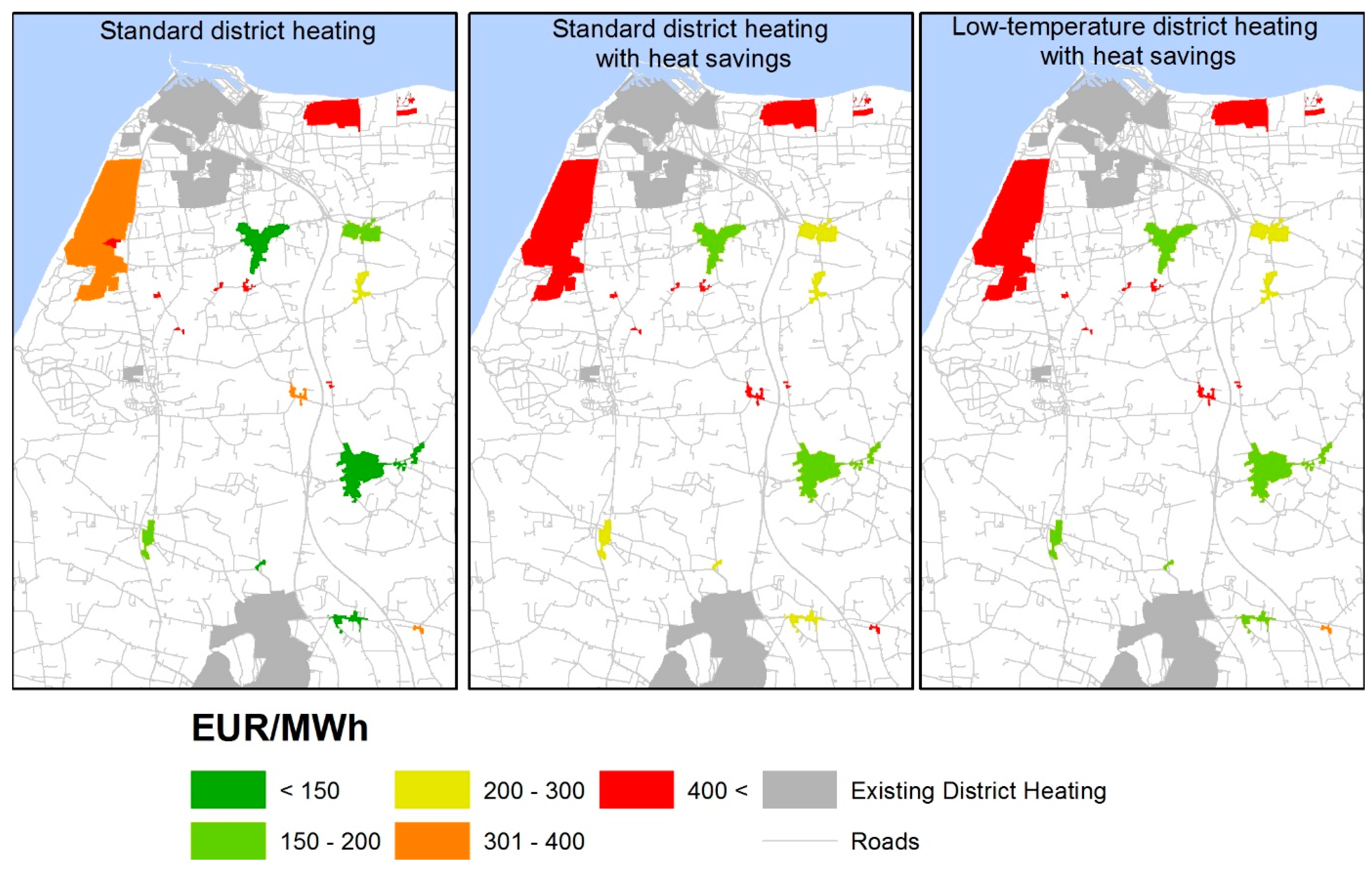
The total number of buildings in the northern region of Denmark that are connected to district heating is 152,979. The number of buildings that are located in towns but do not have district heating is 64,079; there are an additional 151,611 buildings located outside towns that do not have district heating. The only buildings included in this analysis are the 64,079 that are located in towns but do not currently have district heating. Figure 7 shows a part of the output of the GIS model. The existing district heating areas are shown as grey areas, while the potential areas are coloured from green to red, depending on the expected cost in €/MWh for supplying these areas. As described in the methodology, this cost is based on each potential area being connected to the nearest existing district heating area. Figure 7 shows the output for the same area for all three scenarios. It is evident that the expansion potential is largest in the standard district heating scenario. This is because the heat savings implemented in the other two scenarios influence the heat density in each area, which causes the investment costs to become relatively higher. Hence, in the scenario with standard district heating and heat savings, there are only a few remaining areas that offer low-cost expansion potential. In the scenario with low-temperature district heating and heat savings, this is improved slightly, as more areas have low costs.
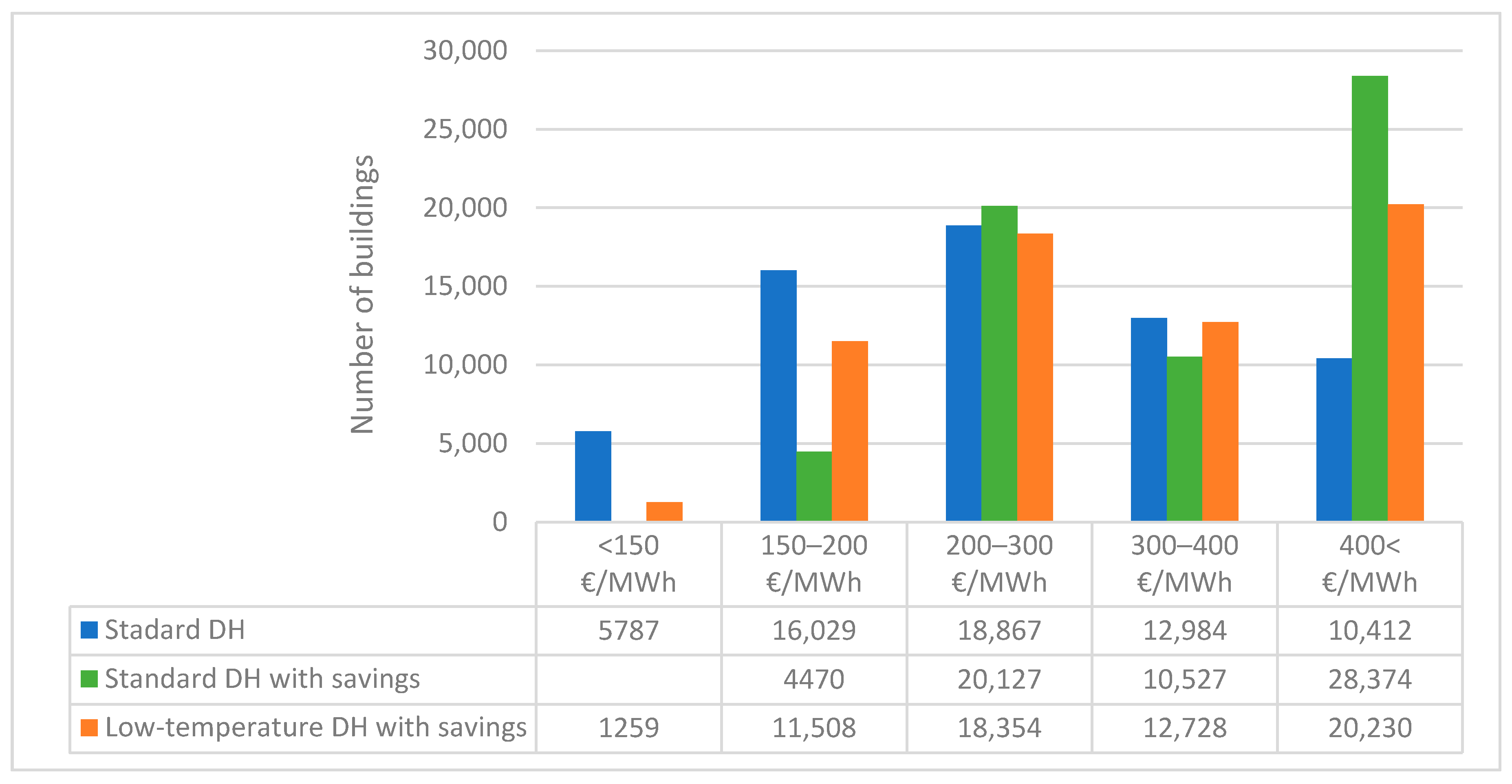
The maps shown in Figure 7 represent a small portion of the model output and do not include all of the analysed areas. In Figure 8, the whole area is included and presented as a column chart with the same cost categories as in Figure 7. The results clearly show that the expansion potential is cheapest in the standard district heating scenario, which has the highest number of buildings in the two cheapest price categories. Meanwhile, in the scenario with district heating and heat savings, there are no buildings left with a cost below 150 €/MWh, and only 4470 buildings remain in the price range between 150–200 €/MWh. Implementing low-temperature district heating increases this by a factor of three, with the total number of buildings in the two cheapest categories equalling 12,767.
The cost level to be competitive with individual heating options, such as ground-source heat pumps or biomass boilers, is around 150 €/MWh. This implies that expanding district heating in this specific example will be a challenge, especially if the high heat saving scenarios become reality. Low-temperature district heating to a small degree solves this; however, low temperatures alone will not make a large difference in the total costs. Other benefits related to low-temperature district heating, such as being able to use cheaper low-temperature heat sources and an improvement in the efficiency of existing production plants, must also be implemented.
The composition of costs for each of the 1001 analysed areas varies considerably, as some have access to low heat prices from the nearest district heating system, some are denser and have lower investment costs for distribution grids, while others have low transmission costs. Therefore, the cost factor (or factors) that makes district heating feasible or not depends highly on the specific area in question. Nevertheless, the average cost in various categories is used as an indicator to see how the difference varies between the three scenarios; this is illustrated in Figure 9. The heat price on average has a 42% share of the total cost in the standard scenario; this drops when implementing heat savings and lowering temperatures. Instead, pipe costs have an increasingly more significant role, where the costs for distribution and transmission pipes increase from 16% and 28% in the standard scenario to 21% and 33% in the low-temperature scenario with heat savings.
The total annual cost for each scenario is reduced, from 226 M€ in the standard scenario to 197 M€ in the savings scenario and 169 M€ in the low-temperature scenario. This, however, does not include the investment costs for building improvements, so it cannot be used to determine if one scenario is more feasible. It does, however, indicate that there are benefits to reducing heat costs and heat losses in the grids.
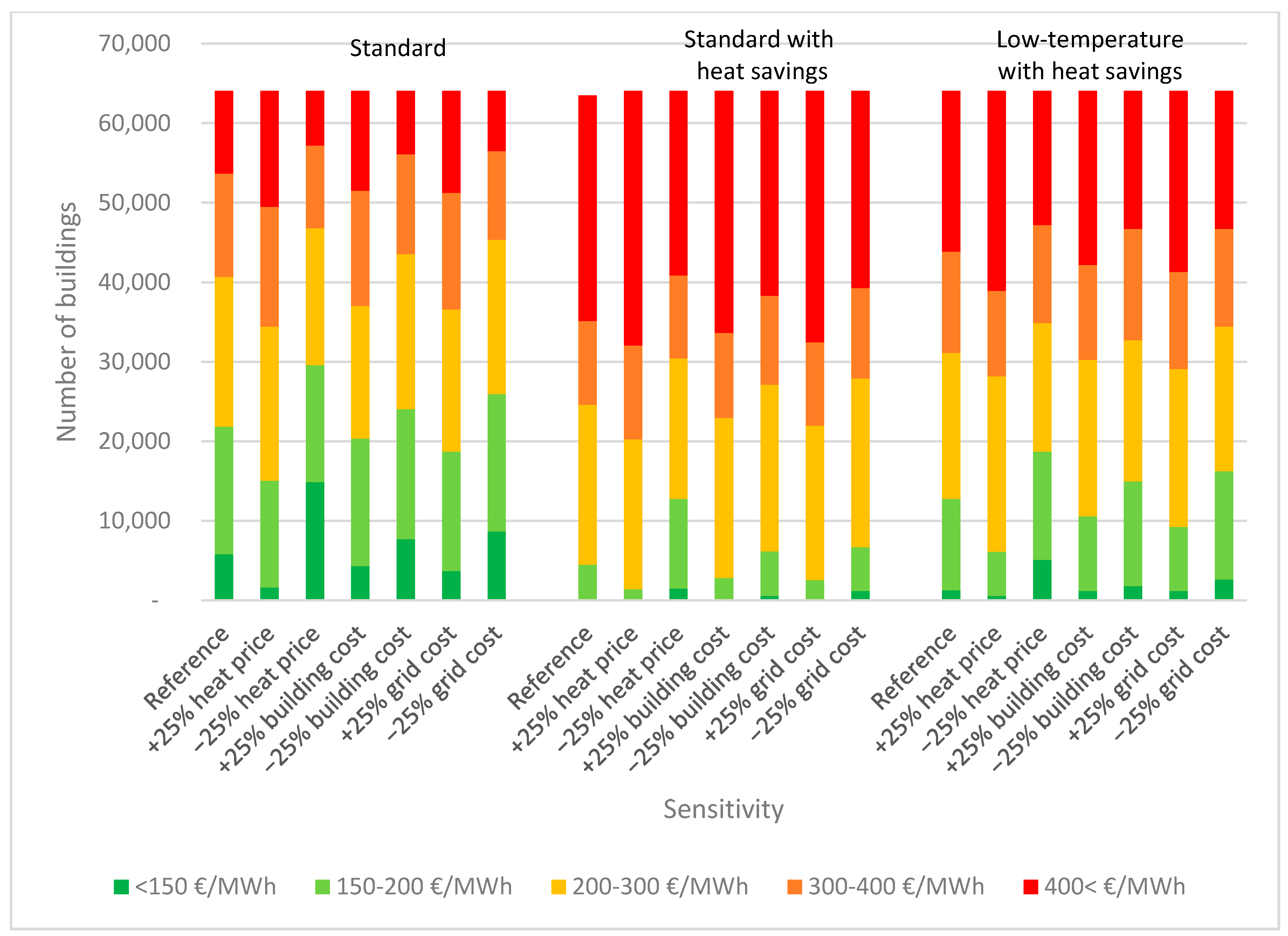
To investigate the impact of different costs further, the critical parameters were analysed in a sensitivity analysis, as shown in Figure 10. The critical parameters are heat price, grid investment costs, and building investments. Adjusting each of these by ±25% shows the impact of each parameter on how many buildings end up in each price category.
The sensitivity analysis shows that changing each of the three parameters does not change the fact that the standard scenario still ends up with the highest number of buildings at a price below 200 €/MWh. The sensitivity analysis also shows that the low-temperature scenario has buildings with prices below 150 €/MWh as well as in the 150–200 €/MWh category in all cases. Meanwhile, the standard scenario with heat savings performs similarly to the reference case, resulting in almost no buildings with a price below 200 €/MWh. However, when considering a 25% price reduction on any parameter, around 5000–12,000 buildings end up in the price range of 150–200 €/MWh for the heat savings scenario. In general, the sensitivity analysis does not change the overall results that district heating has the highest potential in the standard scenario, the lowest potential in the scenario introducing heat savings and a slightly better potential in the low-temperature scenario.
5. Discussion
The example shows how the heat atlas can be used to assess district heating potential. However, there are some uncertainties with respect to the data quality of the heat atlas. As discussed in the model description, even similar buildings rarely have the same heat demand. In the heat atlas, this is solved by using the mean value of different building categories, assuming that the variation in demand will even out over large areas. This assumption implies that the heat atlas becomes less valid as the size of the examined area decreases, because the variation in individual building demand becomes higher. In this article’s example, some areas include very few buildings; in such small areas, the actual heat demand can be expected to vary from the average. This uncertainty is to some degree offset by using a conservative estimate with a minimum distribution pipe size of 48.3 mm, since even smaller pipes could be used in cases with low demand. Moreover, small areas tend not to have much district heating potential due to a low heat demand density compared to the required length of the transmission pipe.
The assessment of distribution grid costs is based on the idea that pipes will be laid following the road network and finding the shortest route for all buildings to a central point in each area. Following the road network is, however, only a general tendency, and sometimes heat networks are built outside roads when deemed feasible. This is something that should be examined when the actual sketching of the network takes place. Hence, the assumption made in this analysis could increase the estimated prices in the GIS model. The placement of the central point is also done automatically and is sometimes placed in areas where restrictions exist; this should not be critical though, as the central point could most likely be placed somewhere close by, thus changing the distribution costs only slightly. Another potential error is the assumption that summing up all the individual routes will give a good estimate of the entire network. A cheaper distribution grid for the whole area could potentially be found by using an optimization model. However, as the model presented in this article is only intended to be used as a screening tool, the chosen method still gives a good indication of the size and costs of distribution grids.
The transmission grid model is simpler than the distribution model, and only uses the direct distance between the potential district heating area and the existing district heating area. This means that the model finds the shortest possible route between areas, and could therefore be assumed to underestimate the costs compared to, e.g., following a road network. Another problem with this method is that it ignores waterways and other physical barriers, so the user must take this into account when examining the model output. As there are no such restrictions in the example used in this article, it is not seen as a problem for this specific case. A final limitation in the model regarding the transmission grid is that it considers each new potential area separately. In many cases, the feasibility of a transmission line would be improved if connecting several towns to the same line, instead of building multiple parallel lines.
The methods presented in this article focus on an annual time resolution due to model complexity. Using, e.g., an hourly time resolution could give more insight into the influence of renewable energy integration or of the peak heat demand in buildings when introducing heat savings. The latter is important when sizing the supply pipes, as the peak heat demand influences the required pipe size. The method presented here takes this into account by using a lower utilization rate to estimate the capacities of pipes when heat savings are introduced. The methods presented here are intended for planning purposes; if someone decides to use these methods to find a potential district heating area, it is highly recommended to conduct a more detailed analysis to determine if the proposed system is indeed feasible.
The heat prices are possibly the cost input with the greatest uncertainty, as they are based on current prices within each district heating area. These prices can be expected to change over time, thus influencing the feasibility of any grid expansion. However, it is hard to guess how the prices will change, as this involves a combination of various factors. For instance, the prices depend on how the different technologies used for heat production are taxed. In addition, most district heating areas have a combined heat and power plant, for which the heat production price depends on the development of the electricity market prices. The grid expansions themselves can also affect the heat production costs, particularly in cases where additional production capacity is required. On the other hand, forces are also pulling the other way; for example, as more subsidies are given for certain types of renewable energy, they could offer cheaper sources of heat than the current supply. Implementing low-temperature district heating could also enable supply companies to invest in heat sources that can be used more efficiently at lower temperatures, such as geothermal, industrial excess and solar thermal production. Another neglected aspect with respect to heat prices is that this analysis only examines the consumer perspective, thus neglecting the added value for society of having district heating. District heating fits well into a future smart energy system [1], as it can implement large amounts of renewable energy sources that cannot be used on a small scale individual basis. District heating also enables a low-cost storage option for regulating wind and other fluctuating renewable energy sources [2]. Furthermore, district heating does not require substantial investments in the electricity grid, as would be necessary if relying on individual heat pumps [25,40].
The general conclusion that district heating becomes more expensive per delivered unit of heat in a future scenario with end-user heat savings does not only apply for district heating. The same tendency goes for all heating systems in which the investment costs cannot be reduced by the same rate as the reduction in yearly heat demand. The result will be a higher share of fixed costs which in Figure 9 is represented by the building cost, distribution pipes and transmission pipe. Therefore, the price of the heat will be a smaller share of the total costs and when the yearly costs are divided by the heat consumption the price per unit of heat will increase. However, the total cost for the building owners will be lower.
A final discussion point involves the case example used in this article. In general, Denmark is not the best case for showing district heating expansion potentials, as many of the best areas for district heating have already been developed. The example of the northern region of Denmark is used to illustrate how the potential can be assessed and how heat savings and low-temperature district heating influences this potential. The example should not be used to generalise the feasibility of district heating, neither in Denmark nor in other countries. The feasibility of district heating depends heavily on local conditions regarding both heat production costs and the heat demand density in the given areas. As neither of these factors are fixed over time, the potential will change accordingly. In sum, applying models like the one presented in this paper can offer insight into the possibilities under certain conditions.
6. Conclusions
In future smart energy systems, the systems’ flexibility and ability to integrate sectors are crucial to balance the large amounts of fluctuating renewable energy sources. Hence, a key technology is district heating, which enables the use of new renewable energy sources and helps to balance the system by providing storage options. However, most long-term energy plans include substantial improvements in the building stock, which is intended to reduce the sector’s heat demand. This reduction challenges the feasibility of district heating systems, because the heat density will be lower, thereby increasing the relative share of investment costs and heat losses. On the other hand, this could also present an opportunity if systems change to the so-called fourth generation of district heating, which uses lower grid temperatures and utilizes a variety of renewable energy sources.
This article looks into this challenge by examining the district heating potential for a case example in which both end-use heat savings and low grid temperatures are taken into account. The analysis includes three scenarios: The first is a reference case with standard temperatures and heat demand, the second considers heat savings, while the third considers heat savings in combination with low-temperature district heating.
To evaluate the district heating potential in the three scenarios, both a heat atlas and a GIS model were developed. The heat atlas was constructed based on a statistical analysis of 5.27 million heat measurements from Danish buildings. These measurements were divided into 32 building categories and seven typical construction periods; the mean kWh/m2 heat demand within each category was assumed to represent every building in the respective category. Thus, the heat atlas resulted in an estimate of the heat consumption for all buildings in Denmark on an address level. The second part of the analysis was devoted to the development of a GIS model that can be used to estimate district heating expansion potential. In general, the model uses the heat demand from the heat atlas to propose distribution grids for existing towns, and then calculates the associated costs and heat losses. The heat demands and losses are then used to estimate the transmission line capacity needed to connect the proposed grid to the nearest existing district heating area. Finally, the investment costs and losses related to the transmission line are found, which, together with individual building investments and heat prices, are used to calculate the total cost of supplying a new area with district heating.
This article describes how the model was applied to the northern region of Denmark to examine the three scenarios. The main conclusions are that the district heating potential is highest in the standard scenario without any heat savings. When heat savings are introduced, the cost of district heating expansions, in most cases, will not be feasible. Introducing low-temperature district heating modestly increases the expansion potential, as it reduces the total costs compared to the scenario that includes standard temperatures and heat savings. However, these cost savings are not large enough to make the expansion potential as viable as in the standard case without heat savings. The model is limited to only analysing savings regarding grid loss and investment cost reductions. A sensitivity analysis was conducted on costs for grids, building installation and heat prices. The results showed that if any of these factors could be reduced, the district heating potential would increase. It is very likely that these costs would be lower in reality, as the model does not include all benefits related to low-temperature district heating. Moreover, there are additional benefits to low-temperature district heating beyond those related to the sensitivity analysis, which could increase the district heating potential even further, such as improving the efficiency of heat production and allowing for the use of cheaper renewable energy sources.
Acknowledgments
The work presented in this paper is a result of the research activities of the Strategic Research Centre for 4th Generation District Heating (4DH), which has received funding from Innovation Fund Denmark (0603-00498B). The research also took place as part of the Heat Roadmap Europe project, which is supported by the European Commission's Horizon 2020 Programme (project number: 695989).
Author Contributions
Both authors conceived and designed the initial study design; Steffen Nielsen ran the GIS simulations. Both authors participated in analysing the data and writing the paper.
Conflicts of Interest
The authors declare no conflict of interest. The founding sponsors had no role in the design of the study; in the collection, analyses, or interpretation of data; in the writing of the manuscript, and in the decision to publish the results.
References
- Mathiesen, B.V.; Lund, H.; Connolly, D.; Wenzel, H.; Østergaard, P.A.; Möller, B.; Nielsen, S.; Ridjan, I.; Karnøe, P.; Sperling, K.; et al. Smart Energy Systems for coherent 100% renewable energy and transport solutions. Appl. Energy 2015, 145, 139–154. [Google Scholar] [CrossRef]
- Lund, H.; Østergaard, P.A.; Connolly, D.; Ridjan, I.; Mathiesen, B.V.; Hvelplund, F.; Thellufsen, J.Z.; Sorknæs, P. Energy Storage and Smart Energy Systems. Int. J. Sustain. Energy Plan. Manag. 2016, 11, 3–14. [Google Scholar] [CrossRef]
- Werner, S. International review of district heating and cooling. Energy 2017, 137, 617–631. [Google Scholar] [CrossRef]
- Li, Y.; Chang, S.; Fu, L.; Zhang, S. A technology review on recovering waste heat from the condensers of large turbine units in China. Renew. Sustain. Energy Rev. 2016, 58, 287–296. [Google Scholar] [CrossRef]
- Duquette, J.; Wild, P.; Rowe, A. The potential benefits of widespread combined heat and power based district energy networks in the province of Ontario. Energy 2014, 67, 41–51. [Google Scholar] [CrossRef]
- Muñoz, M.; Garat, P.; Flores-Aqueveque, V.; Vargas, G.; Rebolledo, S.; Sepúlveda, S.; Daniele, L.; Morata, D.; Parada, M.Á. Estimating low-enthalpy geothermal energy potential for district heating in Santiago basin-Chile (33.5°S). Renew. Energy 2015, 76, 186–195. [Google Scholar] [CrossRef]
- Xiong, W.; Wang, Y.; Mathiesen, B.V.; Zhang, X. Case study of the constraints and potential contributions regarding wind curtailment in Northeast China. Energy 2016, 110, 55–64. [Google Scholar] [CrossRef]
- Frederiksen, S.; Werner, S. District Heating and Cooling; Studentlitteratur: Lund, Sweden, 2013. [Google Scholar]
- Thellufsen, J.Z.; Lund, H. Energy saving synergies in national energy systems. Energy Convers. Manag. 2015, 103, 259–265. [Google Scholar] [CrossRef]
- Hansen, K.; Connolly, D.; Lund, H.; Drysdale, D.; Thellufsen, J.Z. Heat Roadmap Europe: Identifying the balance between saving heat and supplying heat. Energy 2016. [Google Scholar] [CrossRef]
- D’Agostino, D.; Zangheri, P.; Castellazzi, L. Towards Nearly Zero Energy Buildings in Europe: A Focus on Retrofit in Non-Residential Buildings. Energies 2017, 10, 117. [Google Scholar] [CrossRef]
- Patiño-Cambeiro, F.; Armesto, J.; Patiño-Barbeito, F.; Bastos, G. Perspectives on Near ZEB Renovation Projects for Residential Buildings: The Spanish Case. Energies 2016, 9, 628. [Google Scholar] [CrossRef]
- David, A.; Mathiesen, B.V.; Averfalk, H.; Werner, S.; Lund, H. Heat Roadmap Europe: Large-Scale Electric Heat Pumps in District Heating Systems. Energies 2017, 10, 578. [Google Scholar] [CrossRef]
- Lund, H.; Werner, S.; Wiltshire, R.; Svendsen, S.; Thorsen, J.E.; Hvelplund, F.; Mathiesen, B.V. 4th Generation District Heating (4GDH). Integrating smart thermal grids into future sustainable energy systems. Energy 2014, 68, 1–11. [Google Scholar] [CrossRef]
- Lund, R.; Østergaard, D.S.; Yang, X.; Mathiesen, B.V. Comparison of Low-temperature District Heating Concepts in a Long-Term Energy System Perspective (In review). Int. J. Sustain. Energy Plan. Manag. 2017, 12, 5–18. [Google Scholar]
- Østergaard, P.A.; Andersen, A.N. Booster heat pumps and central heat pumps in district heating. Appl. Energy 2016. [Google Scholar] [CrossRef]
- The City of Paris Paris Heat Map. Available online: http://www.paris.fr/pratique/environnement/energie-plan-climat/carte-de-la-thermographie-a-paris/rub_8411_stand_91543_port_19606 (accessed on 20 November 2011).
- Greater London Authority London Heat Map. Available online: https://www.london.gov.uk/what-we-do/environment/energy/london-heat-map/view-london-heat-map (accessed on 23 January 2018).
- Wyrwa, A.; Chen, Y. Mapping Urban Heat Demand with the Use of GIS-Based Tools. Energies 2017, 10, 720. [Google Scholar] [CrossRef]
- Østergaard, P.A.; Mathiesen, B.V.; Möller, B.; Lund, H. A renewable energy scenario for Aalborg Municipality based on low-temperature geothermal heat, wind power and biomass. Energy 2010, 35, 4892–4901. [Google Scholar] [CrossRef]
- Long-Term Heat Plan for Greater Copenhagen. Available online: http://www.varmeplanhovedstaden.dk/ (accessed on 23 January 2018).
- Mathiesen, B.V.; Hansen, K.; Ridjan, I.; Lund, H.; Nielsen, S. Samsø Energy Vision 2030—Converting Samsø to 100% Renewable Energy. Available online: http://vbn.aau.dk/files/220291121/Sams_report_20151012.pdf (accessed on 23 January 2018).
- Dyrelund, A.; Lund, H.; Möller, B.; Mathiesen, B.V.; Fafner, K.; Knudsen, S.; Lykkemark, B.; Ulbjerg, F.; Laustsen, T.H.; Larsen, J.M.; et al. Heat plan Denmark (Varmeplan Danmark). Available online: http://vbn.aau.dk/files/16591725/Varmeplan_rapport.pdf (accessed on 23 January 2018).
- Xiong, W.; Wang, Y.; Mathiesen, B.V.; Lund, H.; Zhang, X. Heat roadmap China: New heat strategy to reduce energy consumption towards 2030. Energy 2015, 81, 274–285. [Google Scholar] [CrossRef]
- Connolly, D.; Mathiesen, B.V.; Østergaard, P.A.; Möller, B.; Nielsen, S.; Lund, H.; Persson, U.; Werner, S.; Grözinger, J.; Boermans, T.; et al. Heat Roadmap Europe 2: Second Pre-Study for the EU27. Available online: http://vbn.aau.dk/files/77342092/Heat_Roadmap_Europe_Pre_Study_II_May_2013.pdf (accessed on 23 January 2018).
- Persson, U.; Möller, B.; Werner, S. Heat Roadmap Europe: Identifying strategic heat synergy regions. Energy Policy 2014, 74, 663–681. [Google Scholar] [CrossRef]
- Nielsen, S.; Lykkemark, B. District Heating Analysis Central Region Denmark. Available online: https://www.rm.dk/siteassets/regional-udvikling/ru/publikationer/energi/fjernvarmeanalyse-afgraensning.pdf (accessed on 23 January 2018).
- Nielsen, S.; Möller, B. GIS based analysis of future district heating potential in Denmark. Energy 2013, 57, 458–468. [Google Scholar] [CrossRef]
- Nielsen, S. A geographic method for high resolution spatial heat planning. Energy 2014, 67, 351–362. [Google Scholar] [CrossRef]
- Grundahl, L.; Nielsen, S.; Lund, H.; Möller, B. Comparison of district heating expansion potential based on consumer-economy or socio-economy. Energy 2016, 115, 1771–1778. [Google Scholar] [CrossRef]
- Möller, B. A heat atlas for demand and supply management in Denmark. Manag. Environ. Qual. Int. J. 2008, 19, 467–479. [Google Scholar] [CrossRef]
- Möller, B.; Nielsen, S. High resolution heat atlases for demand and supply mapping. Int. J. Sustain. Energy Plan. Manag. 2014, 1, 41–58. [Google Scholar]
- The European Commission. Directive 2010/31/EU of the European Parliament and of the Council of 19 May 2010 on the Energy Performance of Buildings; European Commission: Brussels, Belgium, 2010. [Google Scholar]
- Ministry of Housing and Urban and Rural Affairs Energy Consumption Data in the Building Register 2012. Available online: http://bbr.dk/energiforbrugsdata (accessed on 23 January 2018).
- Østergaard, D.S.; Svendsen, S. Theoretical overview of heating power and necessary heating supply temperatures in typical Danish single-family houses from the 1900s. Energy Build. 2016, 126, 375–383. [Google Scholar] [CrossRef]
- The Danish Energy Regulatory Authority. Heat Price Statistics—December 2016; The Danish Energy Regulatory Authority: Copenhagen, Denmark, 2016. [Google Scholar]
- The Danish Energy Regulatory Authority. Analysis of District Heating Prices (in Danish). Available online: http://energitilsynet.dk/fileadmin/Filer/0_-_Nyt_site/VARME/Materiale_til_varmenyheder/2013-05_-_Varmeprisanalyse/Varmeprisanalyse.pdf (accessed on 23 January 2018).
- The Swedish District Heating Association. Kulvertkostnadskatalog (The District Heating Pipe Cost Catalogue). Available online: https://www.energiforetagen.se/det-erbjuder-vi/publikationer-och-e-tjanster/fjarrvarme/Kostnadskatalog-fjarrvarme-distribution/ (accessed on 23 January 2018).
- The Danish Energy Agency. Technology Data for Energy Plants: Individual Heating Plants and Technology Transport; Danish Energy Agency and Energinet.dk: Copenhagen, Denmark, 2012. [Google Scholar]
- Pudjianto, D.; Djapic, P.; Aunedi, M.; Gan, C.K.; Strbac, G.; Huang, S.; Infield, D. Smart control for minimizing distribution network reinforcement cost due to electrification. Energy Policy 2013, 52, 76–84. [Google Scholar] [CrossRef] [Green Version]
Figure 1.
Heat demands in building category (a) 110 (Farmhouse and agricultural holding); (b) 120 (Detached single-family house); (c) 130 (Terrace, linked or double house (horizontal separation between units)); (d) 140 (A building of flats (A house for multiple families including two family housing (Vertical separation between units))).

Figure 2.
Heat atlas example showing annual heat demand in buildings.

Figure 3.
District heating consumer prices for all 422 district heating areas in Denmark. Data from [36].
Figure 3.
District heating consumer prices for all 422 district heating areas in Denmark. Data from [36].
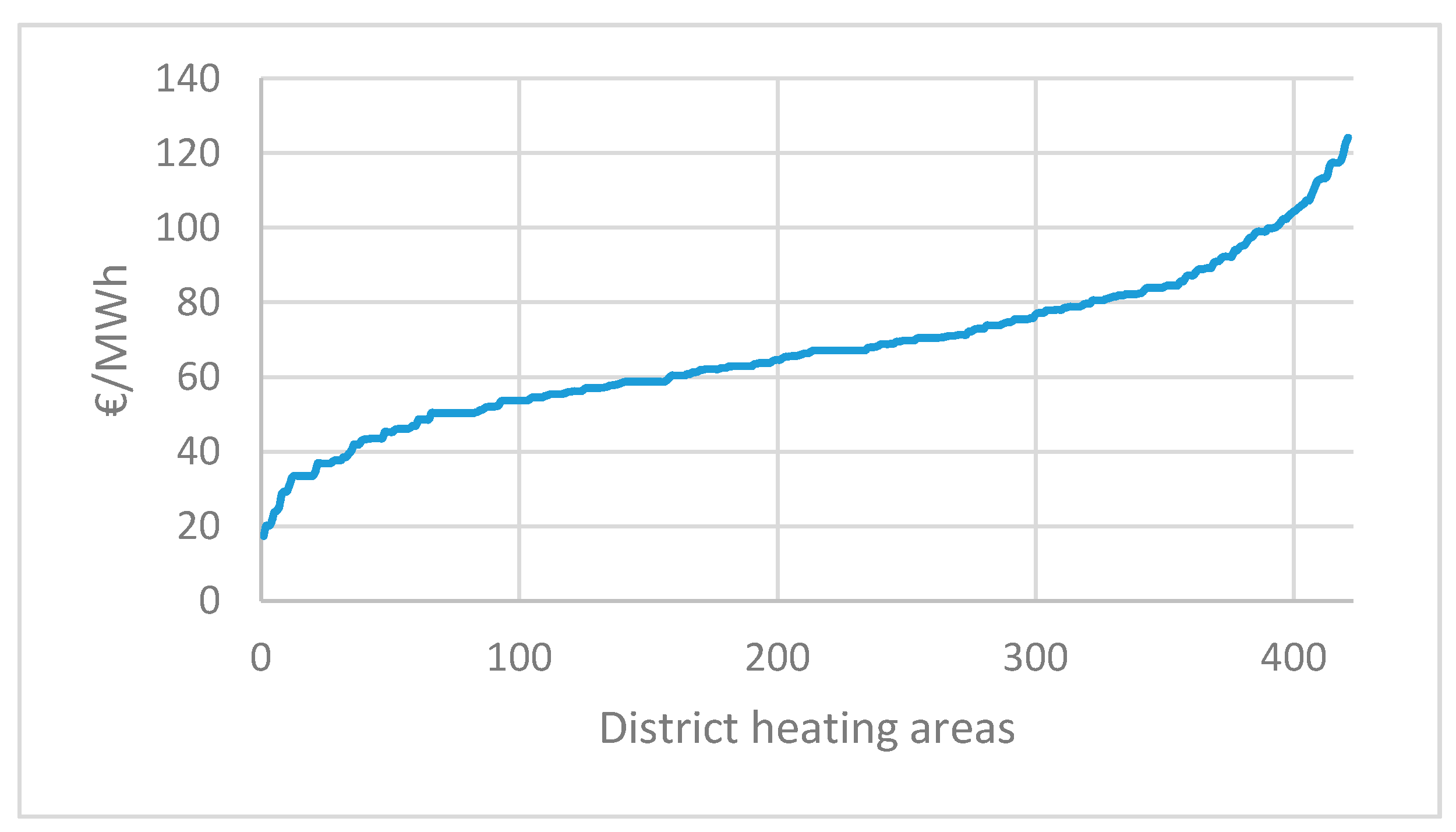
Figure 4.
Investment costs of distribution and transmission pipes. Data from [38].
Figure 4.
Investment costs of distribution and transmission pipes. Data from [38].

Figure 5.
The generalised approach in the GIS (Geographical Information System) model.

Figure 6.
Example of distribution network generated by the model.

Figure 7.
Example of map output for the area of Hirtshals.

Figure 8.
Heat costs for district heating expansion in three scenarios.

Figure 9.
The average percentage share of costs in the three scenarios.

Figure 10.
Sensitivity analysis of critical parameters.


Table 1.
Frequency of measurements categorised by heat supply type and year.
| 2010 | 2011 | 2012 | 2013 | 2014 | |
|---|---|---|---|---|---|
| District Heating | 562,718 | 599,037 | 579,537 | 616,873 | 533,586 |
| Natural Gas | 355,461 | 357,662 | 361,548 | 362,783 | 313,854 |
| Oil | 161,982 | 162,396 | 153,720 | 106,485 | 46,315 |
| Total | 1,080,161 | 1,119,095 | 1,094,095 | 1,086,141 | 893,755 |
Table 2.
Frequency of measurements categorised by building type and year.
| 2010 | 2011 | 2012 | 2013 | 2014 | |
|---|---|---|---|---|---|
| Residential | 978,029 | 1,018,645 | 995,232 | 994,343 | 829,086 |
| Production and Storage | 48,753 | 43,755 | 42,938 | 36,381 | 21,149 |
| Office and trade | 32,090 | 33,942 | 33,899 | 33,612 | 26,741 |
| Public buildings | 12,596 | 13,124 | 13,124 | 13,095 | 10,414 |
| Vacation/holiday | 8693 | 9629 | 9612 | 8710 | 6365 |
| Total | 1,080,161 | 1,119,095 | 1,094,805 | 1,086,141 | 893,755 |
Table 3.
Capacities of different pipe dimensions.
| Pipe Dimension (mm) | Standard (80/40 °C) (MW) | Low-Temperature (55/25 °C) (MW) |
|---|---|---|
| 48.3 | 0.04 | 0.03 |
| 60.3 | 0.08 | 0.06 |
| 76.1 | 0.17 | 0.13 |
| 88.9 | 0.31 | 0.23 |
| 114.3 | 0.59 | 0.44 |
| 139.7 | 0.90 | 0.67 |
| 168.3 | 1.74 | 1.31 |
| 219.1 | 2.99 | 2.24 |
| 273 | 4.90 | 3.67 |
| 323.9 | 9.88 | 7.41 |
| 406.4 | 17.60 | 13.20 |
| 508 | 28.10 | 21.08 |
| 609.6 | 50.99 | 38.25 |
| 711.2 | 91.94 | 68.95 |
| 812.8 | 147.59 | 110.69 |
| 914.4 | 220.91 | 165.68 |
| 1016 | 312.94 | 234.70 |
Table 4.
Estimated heat losses for various dimensions of pipes.
| Pipe Dimension (mm) | Standard (80/40 °C) (W/m) | Low-Temperature (55/25 °C) (W/m) |
|---|---|---|
| 48.3 | 5.29 | 3.25 |
| 60.3 | 6.60 | 4.06 |
| 76.1 | 8.33 | 5.13 |
| 88.9 | 9.73 | 5.99 |
| 114.3 | 12.52 | 7.70 |
| 139.7 | 15.30 | 9.41 |
| 168.3 | 18.43 | 11.34 |
| 219.1 | 23.99 | 14.76 |
| 273 | 29.89 | 18.40 |
| 323.9 | 35.47 | 21.83 |
| 406.4 | 44.50 | 27.39 |
| 508 | 55.63 | 34.23 |
| 609.6 | 66.75 | 41.08 |
| 711.2 | 77.88 | 47.93 |
| 812.8 | 89.01 | 54.77 |
| 914.4 | 100.13 | 61.62 |
| 1016 | 111.26 | 68.47 |
© 2018 by the authors. Licensee MDPI, Basel, Switzerland. This article is an open access article distributed under the terms and conditions of the Creative Commons Attribution (CC BY) license (http://creativecommons.org/licenses/by/4.0/).
Share and Cite
MDPI and ACS Style
Nielsen, S.; Grundahl, L. District Heating Expansion Potential with Low-Temperature and End-Use Heat Savings. Energies 2018, 11, 277. https://doi.org/10.3390/en11020277
AMA Style
Nielsen S, Grundahl L. District Heating Expansion Potential with Low-Temperature and End-Use Heat Savings. Energies. 2018; 11(2):277. https://doi.org/10.3390/en11020277
Chicago/Turabian StyleNielsen, Steffen, and Lars Grundahl. 2018. "District Heating Expansion Potential with Low-Temperature and End-Use Heat Savings" Energies 11, no. 2: 277. https://doi.org/10.3390/en11020277
Note that from the first issue of 2016, this journal uses article numbers instead of page numbers. See further details here.