Design and Performance Evaluation of an Axial Inflow Turbocharger Turbine


1
Centre for Advanced Powertrain and Fuels Research (CAPF), Department of Mechanical, Aerospace and Civil Engineering, Brunel University London, Uxbridge UB8 3PH, UK
2
Metapulsion Engineering Limited, Northwood, Middlesex HA6 2NP, UK
*
Author to whom correspondence should be addressed.
Energies 2018, 11(2), 278; https://doi.org/10.3390/en11020278
Submission received: 22 December 2017
/
Revised: 18 January 2018
/
Accepted: 19 January 2018
/
Published: 24 January 2018
(This article belongs to the Special Issue Recent Advances in Internal Combustion Engines Operation and Emissions)
Abstract
:This paper is focussed on the development of an axial inflow turbocharger turbine as a viable alternative to a baseline radial turbine for certain applications. Additionally a variable geometry turbine (VGT) technology is incorporated into the axial-inflow turbine to additionally benefit both efficiency and performance. The developed turbine was compared to the baseline in terms of engine performance, fuel consumption and emissions. The design and optimisation of the inlet casing, stator and rotor blades for axial inflow turbine were developed through CFD simulation. Then a VGT system was further developed, equipped with pivoting stator blades. Necessary data at various flow conditions were collected for engine modelling to test the engine performance achieved by the integration of the axial turbine, which achieved a maximum 86.2% isentropic efficiency at 102,000 rpm. The paper further focussed on the design and optimization of a volute for axial inflow turbine. Various initial designs were tested using CFD simulations and the chosen configuration was optimised further to improve overall stage efficiency, which reached 81.2%. Engine model simulations demonstrated that engine power and torque are significantly increased through the application of the proposed variable geometry axial turbocharger turbine.
1. Introduction
New vehicles around the globe have to comply with emission legislations which are set by the government bodies, with global warming being the main motivator. Regularly, these emission legislations become stricter, reducing the allowance of CO, NOX, HCs and other emissions for the automotive industry. The main emission standards are defined in Europe currently by Euro VI. European Parliament and the Council set regulation for the maximum value of manufacturer’s fleet average CO2 emission levels, targeting 95 g/km from 2020 [1,2]. If the average value exceeds the limit the manufacturer has to pay monetary penalty for each registered car [3].
Another problem for car manufacturers is the increasing price of oil, which are used by the majority of the vehicles to produce power. At 2018 the price of oil will exceed 60 dollars per barrel and is expected to increase up to 80 dollars by 2030 [4]. This means that the price for petrol and diesel will increase accordingly, leading to demand for more fuel efficient vehicles.
An effective way of generating these improvements in engine efficiency is by means of reducing the displacement of the engine itself, commonly known as engine downsizing. Downsized engines have been developed in order to obtain higher thermal efficiencies which are connected with the reduction of fuel consumption and CO2 emissions. The engine then operates at a higher efficiency point due to being forced to operate at a higher specific load. To achieve higher specific loads the implementation of a boosting system is mandatory, as in this way forced induction can be achieved allowing a higher specific power to be achieved from a comparatively smaller power unit.
One of the main issues related to turbochargers is turbocharger lag at low exhaust flow rates as the turbine received insufficient flow of gas resulting in slow response to engine acceleration commands [5]. During this period the efficiency and performance of an engine is decreased and emissions are increased. This brings the need to improve turbocharger efficiency at low exhaust gas mass flow rates.
There are a number of ways to reduce the turbo lag. The most common, currently, is to use variable geometry turbochargers (VGTs). Commonly in this system, rotatable vanes restrict the flow of exhaust gases and act as nozzles to increase the flow speed, which leads to a higher rotational speed of the turbine wheel compared to a fixed geometry turbine [6]. Currently, electrically-assisted turbochargers are increasingly being investigated for implementation whereby an electric motor is used to accelerate the turbocharger shaft assembly by re-using electrical energy stored in the battery [7]. Another, simpler, way to reduce turbo lag is to reduce the weight of the turbine wheel or in other words to reduce its moment of inertia. This can be achieved by various turbine rotor design techniques or also by replacing the radial turbine with an axial flow equivalent, which has a lower moment or inertia while being able to handle the same flow conditions. Axial turbines are commonly used in marine and aviation applications, but more recently there has been a recurrence of the axial turbine type in automotive use [8,9].
Ultimately the purpose of this investigation was on the improvement of in the operational benefits that can be accrued through the use of this type of turbine by implementing a variable geometry system in its operation. The aim was to computationally determine how the proposed variable geometry axial turbine performs under engine operating conditions of interest while comparing these to experimentally available datasets [10]. The engine in question was chosen to be a Ford Ecoboost 1.6 L. The eventual aim of this study was to prove the combination of VGT and an axial turbine in achieving a reduction in turbocharger lag and the improvement of efficiency of the turbine leading to lower emissions, higher fuel efficiency and performance of a small gasoline engine. As a result, an insight into the potential benefits that an axial-inflow turbine bring to the automotive powertrain in terms of efficiency when applied in smaller, more economical engines is demonstrated.
In the present paper the optimization of the stator and rotor blades of an axial-inflow turbocharger turbine are tackled with a second part presenting the results of this work with respect to the specific design outcomes of the bespoke turbine inlet casing required to achieve high performance.
2. Axial Inflow Preliminary Blade Design
The preliminary design establishes the foundation from which the geometric parameters of turbomachinery can be calculated and analysed providing a foundation from which specific parameters can be designed and optimised from. The preliminary design of a turbocharger was carried out using the operating parameters of a comparable turbine as the basis for the new innovated design. A conventional methodology with calculations of the blade height, angles and aspect ratio, generating the required velocity diagrams was used.
The main geometrical parameters that obtained from the preliminary design calculations include a range of geometrical parameters in regard to the profile of the blades which would be best suited for the turbine conditions in terms of operating mass flow rate, pressures and temperatures at chosen design points.
The main assumptions assigned during the initial preliminary design calculations were that for a low blade tip-to-root ratio, the mean profile of the blade represented the average flow characteristics of the flow properties through this turbine stage. Additionally the net work produced by the turbine was balanced by the work consumed by the compressor impeller, (considering also the mechanical efficiency loss in the bearing system as well [11]).
Based on the mass flow rate of the fluid and the area upon which it enters the turbine the initial absolute velocity can be calculated with the flow entering an axial turbine being in an axial direction [12]. Exhaust gas flow would first come into contact with a row of stator blades used to transform the blade row’s aspect ratio and alter the geometrical area within the turbine housing, optimising the turbine for a range of operating parameters.
The velocity triangles were first calculated at the mean radius using data from baseline turbocharger testing (Table 1), however some assumptions were necessary to complete the calculations (Table 2).
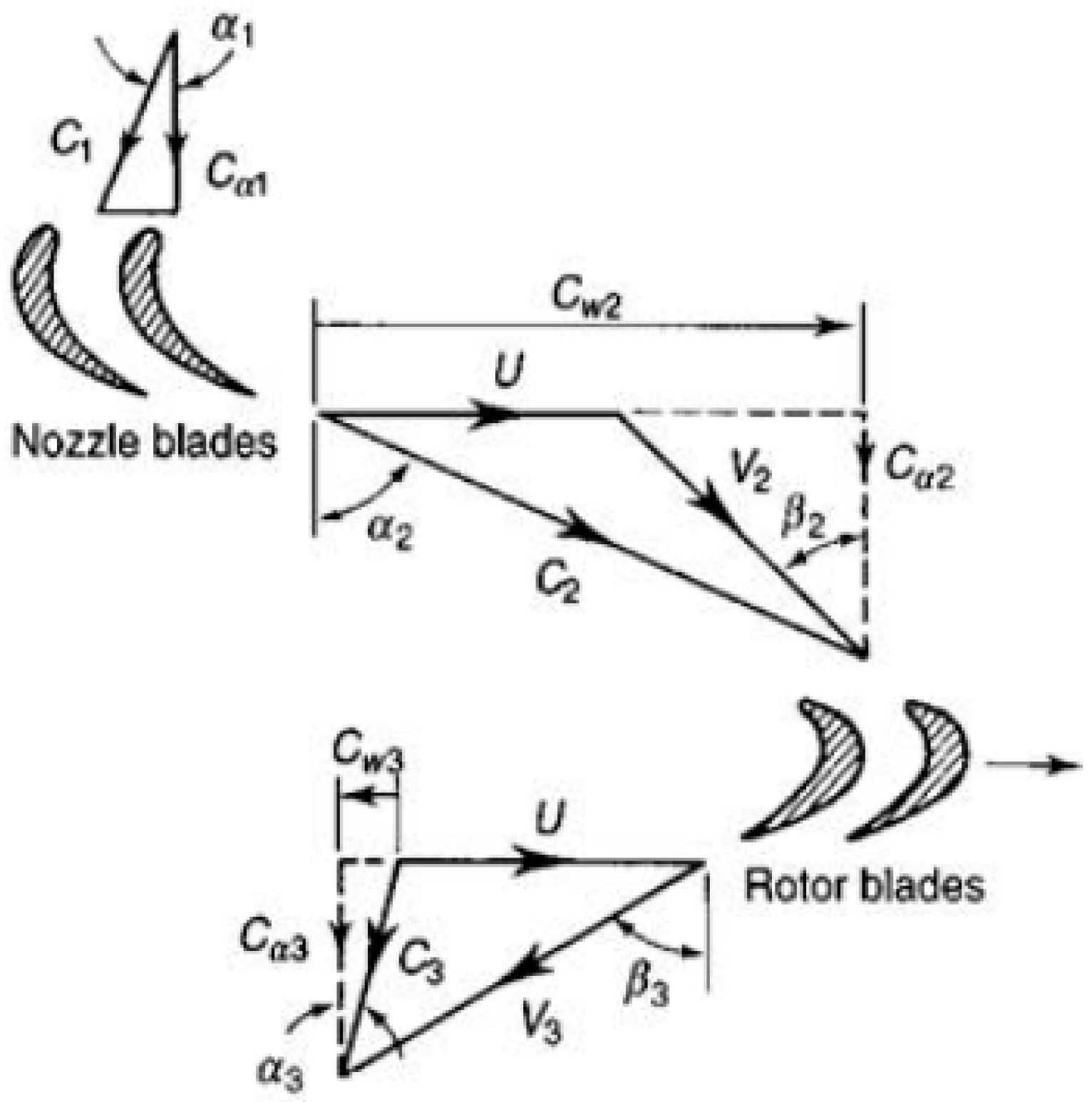
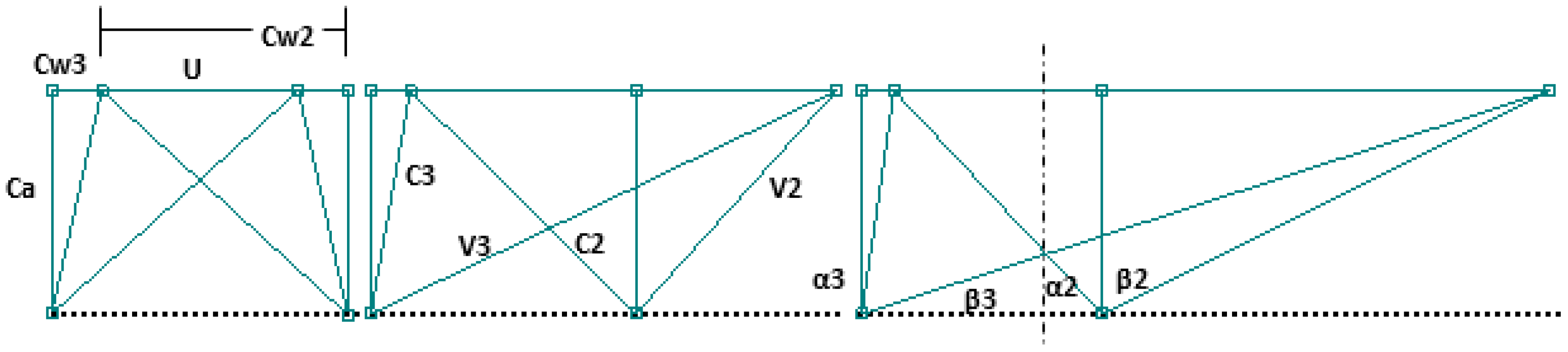
The following equations were used to calculate velocity triangles at the mean radius for maximum exhaust gas flow. The main elements of the nomenclature used can be found in Figure 1:
Once velocity diagram for mean radius is complete the blade height for each section can be calculated:
| Stator Inlet | Rotor Inlet | Rotor Outlet | Blade Radius | ||||
| (9) | (12) | (18) | (22) | ||||
| (10) | (13) | (19) | (23) | ||||
| (11) | (14) | (20) | (24) | ||||
| (15) | (21) | (25) | |||||
| (16) | (26) | ||||||
| (17) |
Once radiuses for root, mean and tip profiles are calculated the free vortex design equations can be used to workout velocity triangles for all three profiles of the blades:
Knowing and all parameters for the velocity diagrams can be calculated using trigonometry through the following schematic representation (Figure 1).
3. Geometric Modelling and Meshing of Turbine Blade Profiles
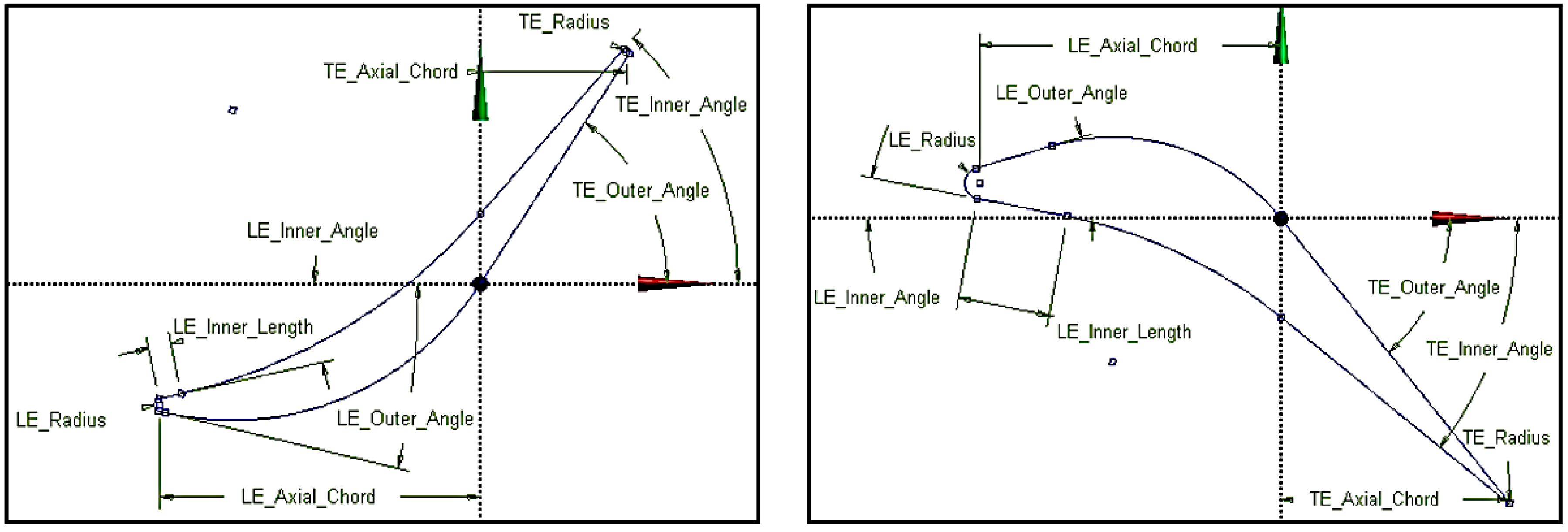
The stator and rotor geometry were created using software package ANSYS Geometry. Blade profiles have cambered aerofoil shapes and were drawn using straight lines and tangential curves as illustrated in Figure 2. The stator blade profile was orientated so as to maximise momentum transfer onto the rotor blades.
Three layers were designed based on their own geometric aerofoil, through the preliminary calculations which would enable this design to be optimised in accordance to the efficiency measured. These were the root, mean and tip sections of the blade. Therefore improvements towards the efficiency of the overall turbine stage could be identified and measured accordingly. Upon the completion of the initial aerofoil, constraints were applied to each measurement of the blade profile, throughout the leading and trailing edges. These constraints were made identical between each layer, ensuring that each measurement could be optimised to the same level detail and accuracy.
From this blade generation, the flow path would be assigned as the domain at which the boundary conditions would be applied. This domain would characterise the mesh generation and allow the analysis of all parameters. Finally the export points were appointed to the blade surface.
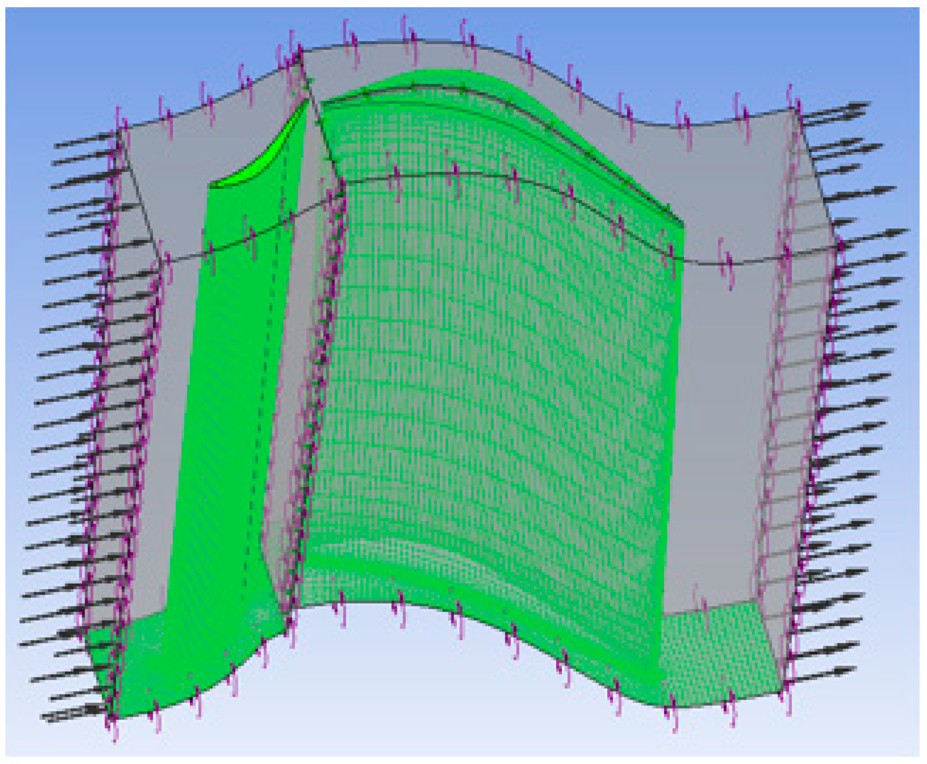
The inlet and outlet boundary can be moved along the length of computational domain in order to define the distance between neighbouring meshes (stator blade or volute) and the actual rotor blade. TurboGrid software was used to generate the topology of the blade, allowing for the user to optimise the mesh (Figure 3). This software is purpose built for turbomachinery applications enabling a higher quality of meshing, including detailed near wall regions in order to investigate the resultant boundary layers and therefore gain a better understanding of the losses through tip clearance which is problematic in turbine development [12].
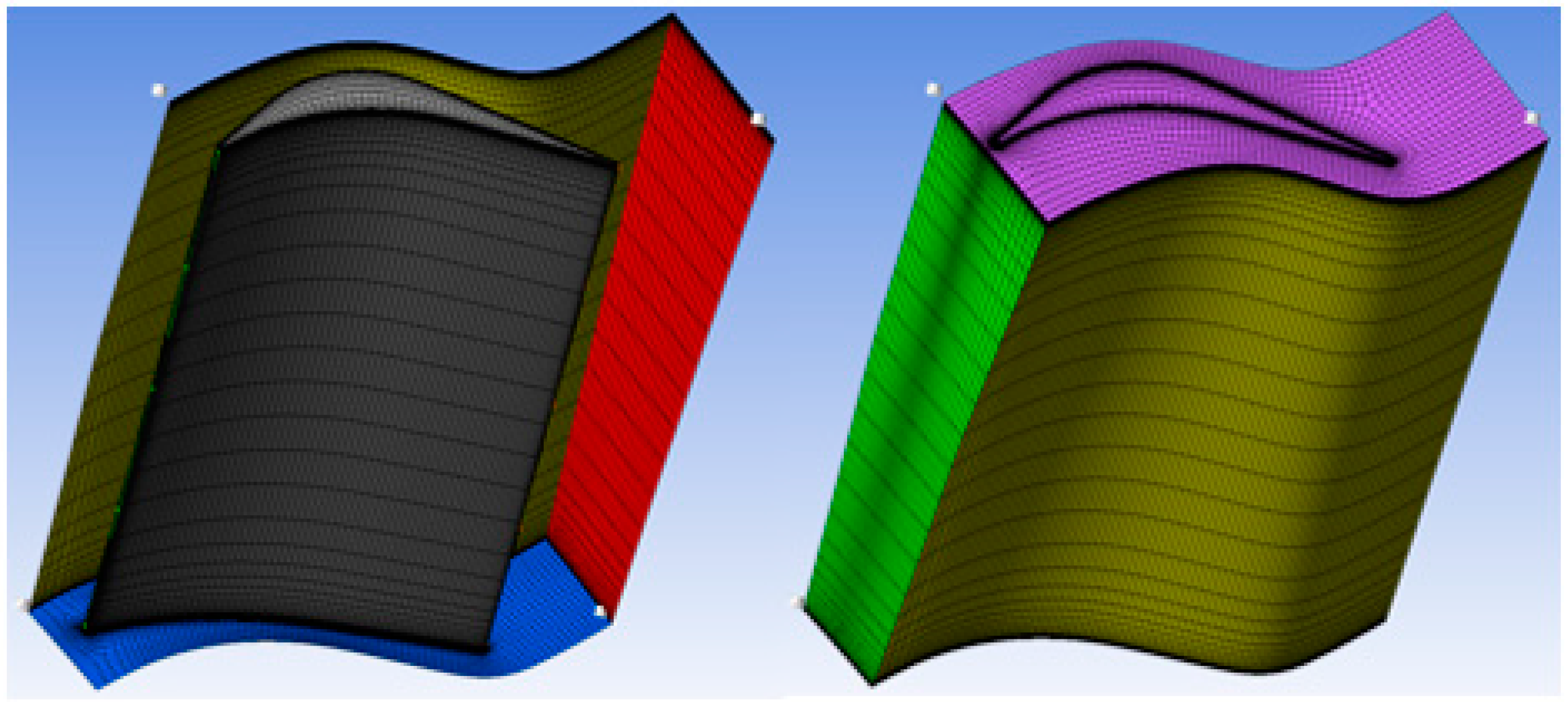
In terms of the clearance area regarding the rotor blades careful consideration must be taken as this is a source of significant overall efficiency loss for the turbine impacting on its ability to convert the kinetic energy of the fluid into mechanical work as a portion of the flow will be able to bypass the rotor blades through flow leakage [13]. Although initially assigned as 0.5 mm, the tip clearance was closely observed through simulations against the respective pressure ratio and efficiency of the turbine. The mesh density proportion would be adjusted with an increasing mesh density applied to the blade under investigation, upon the completion of the optimisation; an equal density for the stator and rotor blades was otherwise applied to maintain a consistent level of accuracy (Figure 4).
4. Arrangement of Boundary Parameters and Simulation Setup
The meshes for stator and rotor were imported into a CFX software setup. First of all those meshes were moved so that outlet of the stator would match the inlet of rotor, but not intersect it (Figure 5). Then stator was defined as a stationary mesh and the rotor was set up as a rotating mesh around the z-axis. A sliding mesh function was used for the rotor and a stationary mesh for the stator domain. To model an accurate representation of the flow’s translation between these two models, translational periodic boundary conditions were established from the stator to the rotor.
For the assignment of the boundary conditions the inlet boundary conditions were adjusted from the GT1548 radial turbocharger turbine experimental test data (used as the basis for this study) due to the updated cross-sectional area of the axial-inflow turbine. The steady-state calculation allowed the resultant change in velocity to be calculated from the expansion of this cross-sectional area and therefore parameters including pressure, temperature and mass flow rate could then be calculated with respect to the geometric area of the axial-inflow turbine in comparison to the GT1548 turbine (using the previously-listed equations). The resultant change in pressure would be calculated based on the difference in area leading to a change in velocity between the two conditions, allowing a comparison to be made between the GT1548 radial turbine and the axial-inflow turbine.
The rotor domain was defined as rotating with air as an ideal gas and a reference pressure of 1 bar; heat transfer was set to total energy and turbulence was set as shear stress transport. The stator mesh was defined similarly but as a stationary domain. The stator inlet was defined with total pressure of 503.93 kPa and heat transfer of total temperature of 880.691 K. The rotor outlet was defined with a mass flow rate of 0.2 kg/s. Walls including the blades were defined as no slip and smooth, but for the rotor shroud the counter rotating wall was selected due to movement of the rotor mesh. The tip of the rotor blade was defined with a general mesh connection which allowed to simulate losses in the clearance between the blade and shroud wall. Because the mesh of a single rotor and stator blade was specified and copied by a number of blades, the connection between these copies was specified as periodic with general mesh connection. The interface between stator and rotor was set as a general connection with a stage mixing plane.
5. Blade Optimisation Procedure
Blades for the stator and rotor built in the preliminary design process were required to be optimised further in order to achieve the highest possible turbine efficiency. It was decided to optimise each parameter at a time and select the one which provides the highest efficiency, implement it and move on to the next parameter.
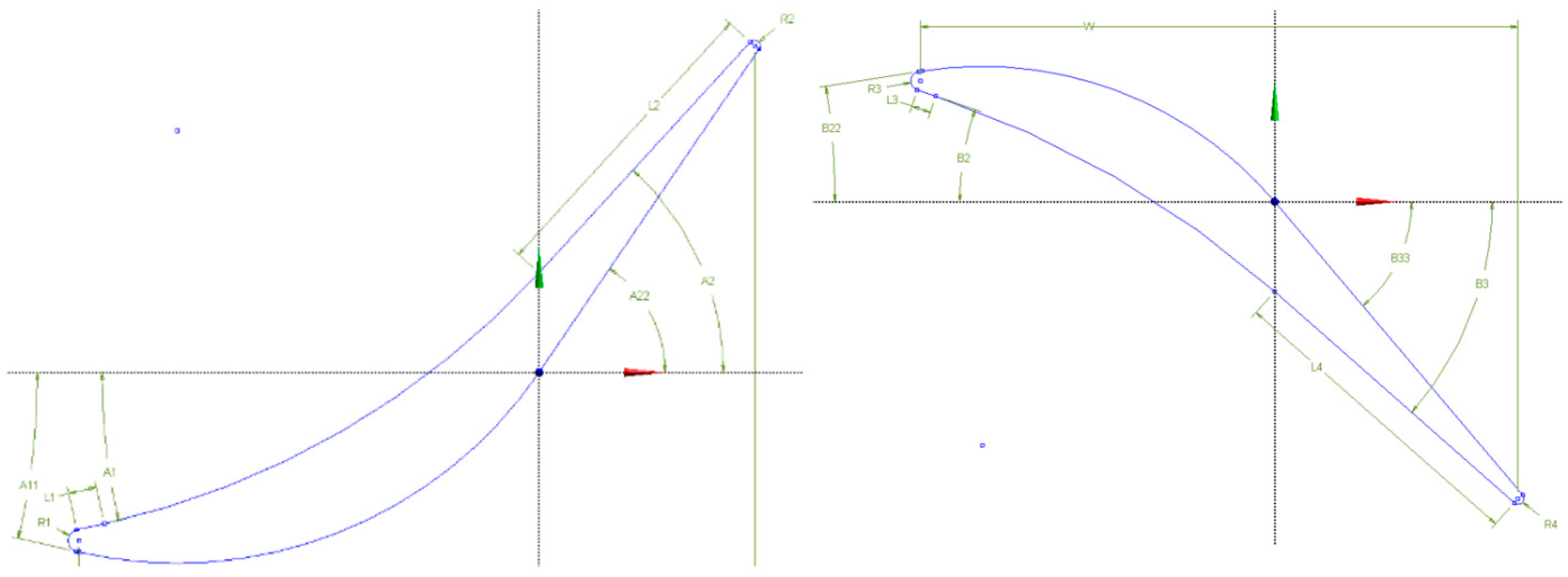
The optimisation begun with selection of a number of blades for the stator and rotor. Once the optimum number of blades was identified the optimisation moved to the stator and rotor blades. Starting with the root and moving to the tip profile of the stator each parameter was optimised in the following sequence (Figure 2): leading inner angle (A1), leading outer angle (A11), leading radius (R1), leading length (L1), trailing length (L2), trailing inner angle (A2), trailing outer angle (A22), trailing radius (R2) and axial chord (W). Similarly, the rotor blade was optimised from root to tip profile: leading inner angle (B2), leading outer angle (B22), leading radius (R4), leading length (L3), trailing length (L4), trailing inner angle (B3), trailing outer angle (B33), trailing radius (R4) and axial chord (W).
6. Volute Design and Optimisation
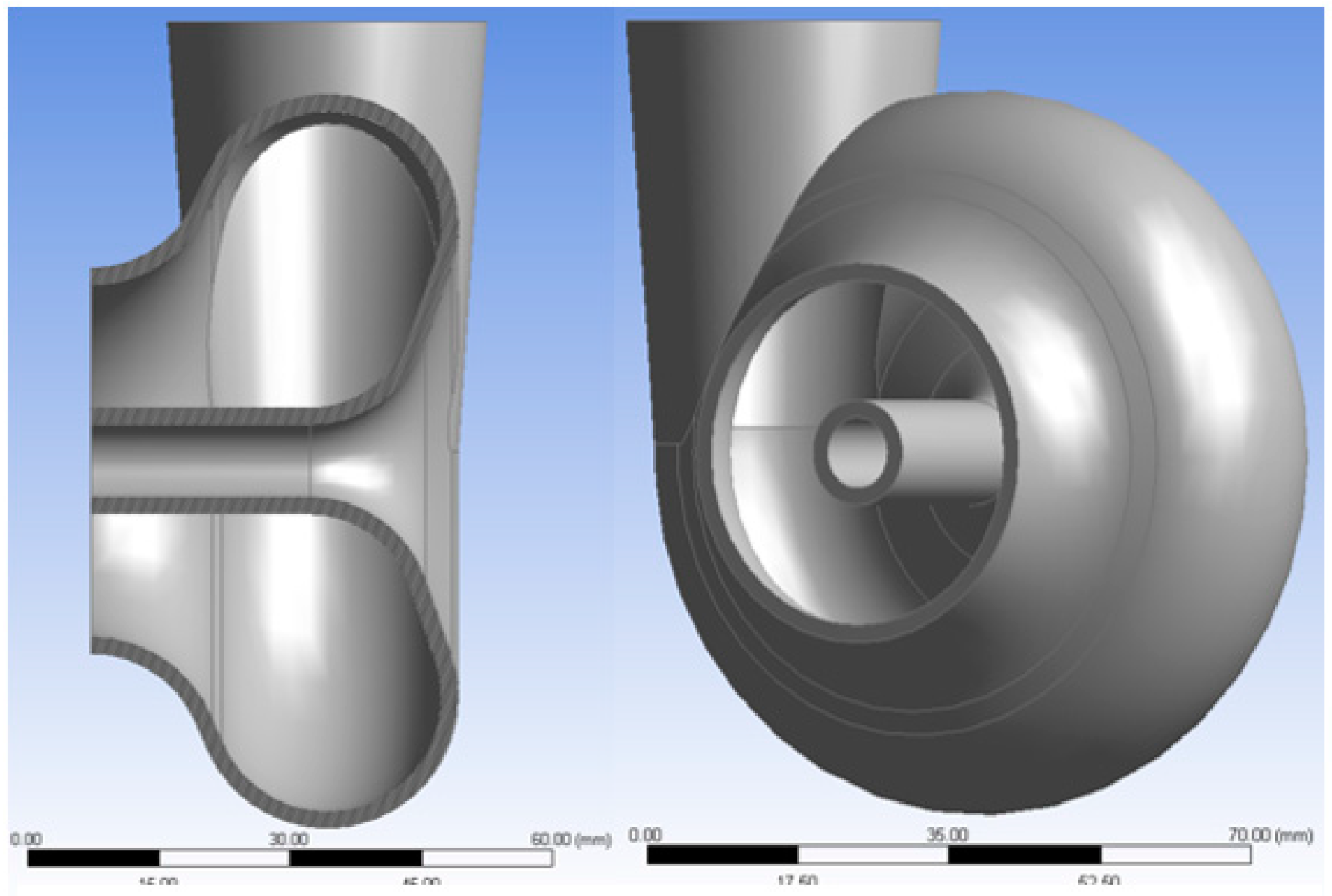
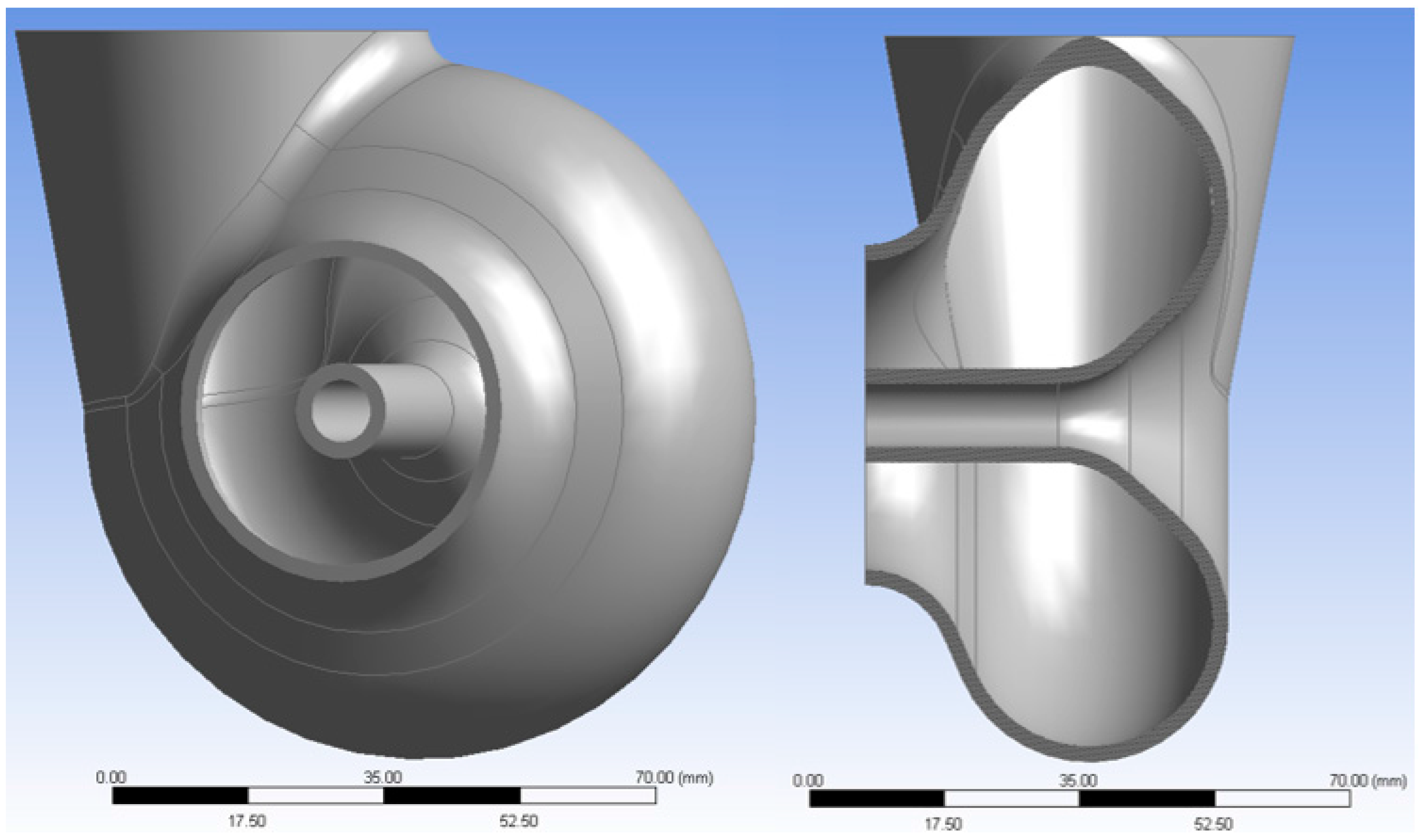
Due to lack of information on volute design principals for axial inflow turbines, four basic designs were created and compared. The first design was based on a standard radial turbine volute with axial inlet and radial outlet, but with uniform radius (Figure 6). The second design was based on the first one but with shorter inlet (Figure 7). The third design was based on the Honeywell axial inflow turbocharger volute from twin turbo system mentioned in the literature review. This design has axial inlet and axial outlet on the side as well as a split inside the volute, which makes it look similar to twin entry volute (Figure 8). However this split has a different role to twin entry design, it supposed to separate flow inside the volute from the flow which exits the turbine rotor in order to reduce back flow. The fourth design has similar principal but the turbine exit is in the radial direction.
Air part was made for all the designs in order to simulate the flow from stator and rotor inside each volute and measure total to static device efficiency, as there were no stages remaining.
In the simulation setup additional interface was introduced between rotor outlet and volute inlet, similar to stator-rotor interface. The volute outlet was defined with mass flow rate of 0.2 kg/s.
Initially four designs of volute were generated. Air part was created for each design in order to simulate volute together with stator and rotor blades. The mesh quality was not good enough due to licence limit of 512 thousand nodes. Number of nodes was reduce for both stator and rotor and was targeted at 100 thousand nodes for each blade. This allowed to use 300 thousand nodes for the volute, however it was not enough due to the volute’s size.
All four designs were simulated together with stator and rotor at 90,000 rpm, however last two designs similar to Honeywell volute were failing during the simulation and no data was collected. This might be due to poor mesh.
The first design provided 73.18% isentropic device efficiency and second design was 41.19% (both together with stator and rotor blades). The first design was chosen for optimisation as it provided highest efficiency.
The first stage of optimisation was to check in which direction volute exit should be placed for highest device efficiency (radial, vertical or axial direction). Volute with axial exit failed during the simulation and no data was collected. Volute with vertical exit was less efficient that one with radial, thus radial exit was selected for further optimisation of volute.
Figure 9 shows main parameters which were optimised for the volute body, however blade height h and radius at the root profile rr were kept constant as rotor and stator blades were already optimised.
Figure 10 shows optimisation progress for volute, where H1 at 25 mm provided efficiency of 75.46%, both R1 at 13 mm and R2 at 12 provided 75.81%, H2 at 29 mm provided 76.64%.
V1 at 27 mm provided efficiency of 76.64% and R3 at 16 mm increased the efficiency up to 77.74% (Figure 11).
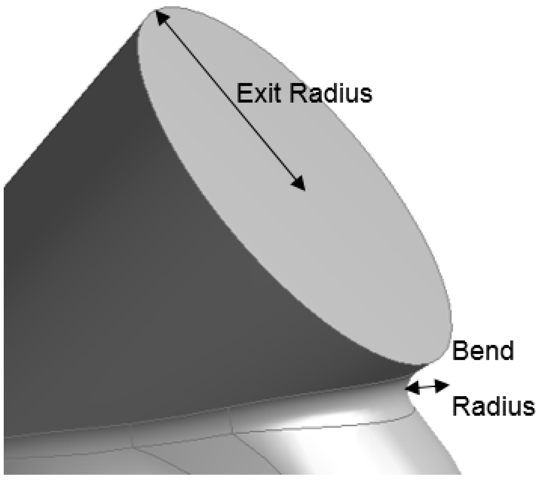
The volute exit parameters like exit radius and bend radius were also optimised (Figure 12). Exit radius of 43 mm provided efficiency of 79.73% and bend radius of 8 mm increased efficiency up to 81.15% (Figure 11).
Overall device efficiency was increased by 10.9% after volute optimisation. Figure 13 shows optimised 3D model of volute for axial inflow turbine.
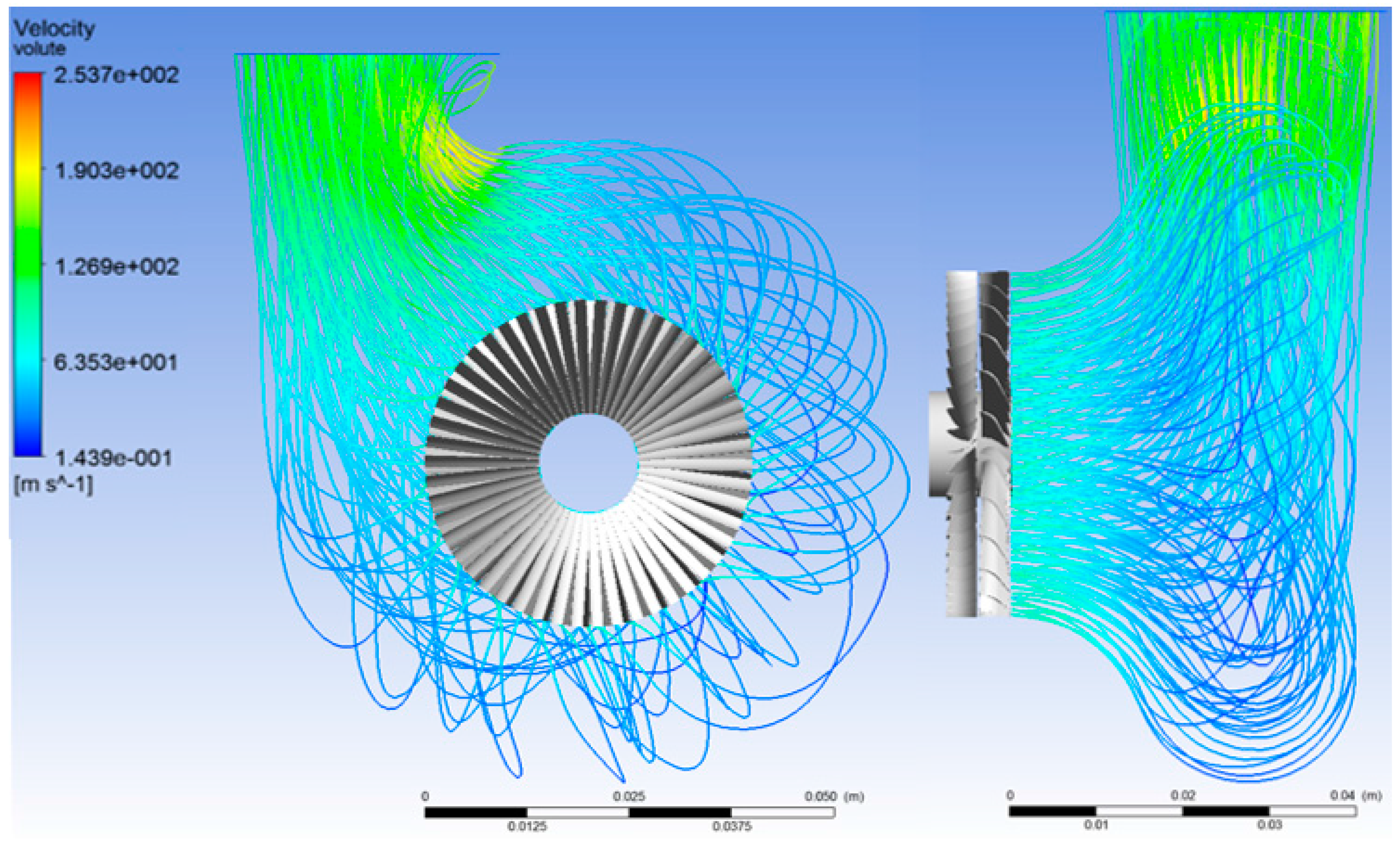
Figure 14 and Figure 15 show simulation results for original and optimised volutes. Both simulations were done with stator and rotor to demonstrate the actual flow streamline evolution inside the volute.
Original volute had rapid increase in the velocity near the exit and flow separation after the bend, which created a separation bubble where no flow exists (next to the yellow streamlines in Figure 14). Optimised volute eliminates separation bubble next to the volute exit and the flow velocity is not rapidly increased at the exit.
7. Variable Geometry Technology Implementation
Incorporating a variable geometry vane system was intended to improve the off-design performance which principally limits the overall efficiency of a generic fixed geometry turbine. During this investigation the pivoting stator vanes were altered in terms of their angular orientation with respect to the horizontal axis, thereby varying the effective area-radius ratio of the turbine.
The pivot angle denotes the angular deflection of the VGT vanes, with the lowest value meaning 0% VGT open area (smallest available area). The lower the velocity of the exhaust gas, the lower the percentage of VGT open area required in order to achieve optimum momentum transfer for any given set of flow conditions. Test data from the baseline turbine were used (Table 3) to calculate boundary conditions at different flow rates as well as dimensions of both turbines (Table 4).
As a result the change in angular velocity of the rotor blade and resultant pressure drop across this single stage against the respective engine loading can be effectively measured. The maximum rotational speed of the turbine can then be determined in relation to the simulated maximum flow rate through CFD, and any additional improvements at separate loading conditions can be measured. As a result of this VGT investigation, five loading conditions were represented with a variable stator profile, measuring the acceleration of the flow from the stator blades into the path of the rotor, with the aim of maximising the turbine’s transient response at part loads.
8. Results
8.1. Preliminary Design Calculations
The preliminary calculations for the axial turbine were based on an existing radial turbine (GT1548 turbocharger). Data collected from an external hot-gas flow test conducted were used as baseline performance map data to compare against the eventual axial turbine design. In addition, boundary, conditions for the preliminary axial turbine design were determined from the experimental test. Fundamental turbine equations could then be solved based on parameters such as the mass flow rate at a given turbine speed. This would allow the calculations of the temperature and pressure located at each station in the turbine stage to be concluded. The degree of reaction was highly dependent of the blades relative loading coefficient which is proportional to the drop in temperature across the two blade rows. However only the turbine inlet temperature was available from the experimental testing, meaning the temperature drop between the inlet and outlet of the turbine could not be accurately calculated. Therefore an assumption of an isentropic temperature drop of 60 K was made; this was based on previous literature regarding a turbine design of an approximate magnitude [14].
As can be seen from Table 5, angles are changing from root to tip. This is due to the free vortex design which reduces losses created by vortices at the root of the blades. Angles A1, A2 and B2 decrease with increasing radius, which means that blades are more twisted at the root and straighten at the tip. However, angle B3 increases towards tip of the rotor blades, creating a more cambered blade profile. Such a profile will produce greater lift on the blades, thus theoretically a higher energy conversion by the rotor.
As mentioned previously, the overall axial turbine dimensions were based on their existing radial turbine equivalent. Therefore during the final design phase an accurate comparison between the two turbines could be performed. As a result the volute nozzle featured a uniform diameter across the area of the blade rows, allowing the location of the mean diameter to be determined as the midpoint between the root and tip as well as the axial cord, for effective packaging (Table 6).
8.2. Generation of Velocity Triangles
The preliminary design allowed the calculation of inlet and outlet velocity triangles, each represented at the different blade profiles considered: root, mean and tip of the blade height (Figure 16).
A number of assumptions were made to ensure an effective representation of the velocity triangles at each profile layer. The first assumption was that the speed relative to the axial direction was to remain constant (Ca1 = Ca2 = Ca3) throughout the turbine and that any changes in this velocity would be in respect to the angular orientation of each blade. Furthermore the angle which distinguishes the stator entrance from the axial direction (α1) is equal to that of the exit of the rotor and axial direction (α3), known as a repeating stage. Although more commonly engineered on multistage turbines this is utilised to describe an identical velocity between inlet and exit by enforcing equal flow angles between these two parameters [14].
Each velocity triangle is comprised of three vectors: rotor blade tip speed (U), absolute flow velocity (C) and the relative velocity of the flow with respect to U (V):
8.3. CFD Blade Optimisation Procedure
To maximise the potential of the proposed axial-inflow turbine for application to the 1.6 L Ecoboost engine the optimum geometric parameters would need to established and analysed, through a fluid dynamic investigation. A frozen rotor model was used for this procedure.
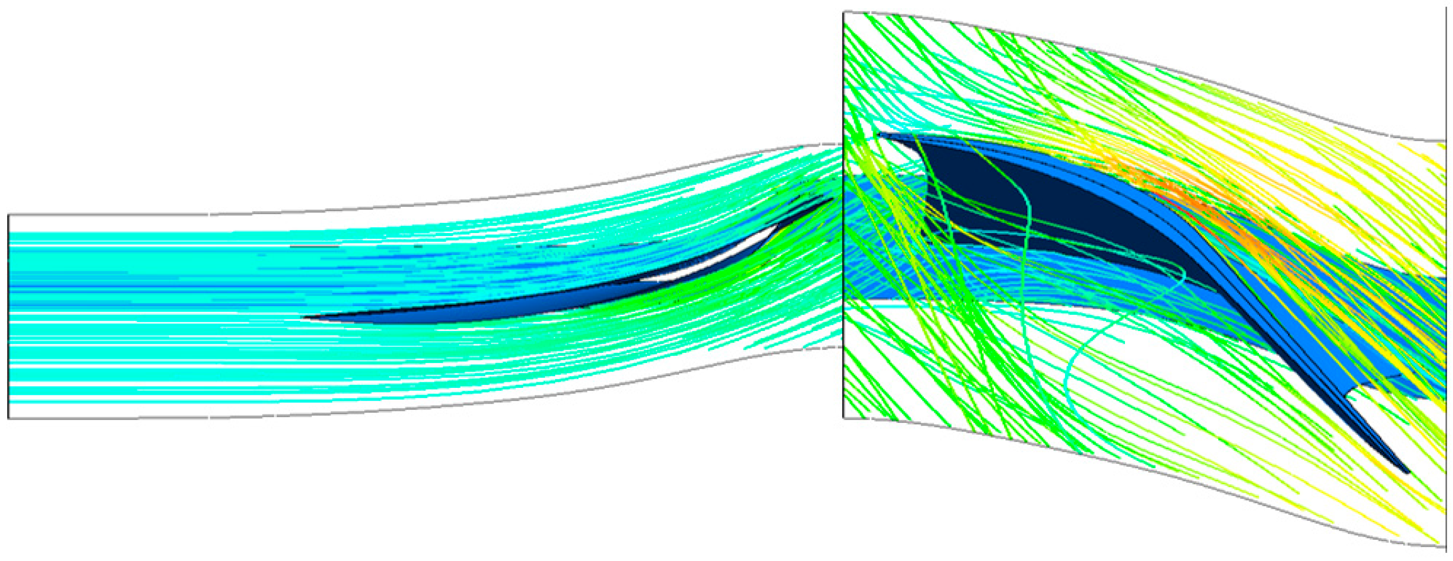
The final preparation before proceeding with the optimisation investigation was to establish the tip speed of the rotor wheel, which will also remain at constant value throughout the investigation, maintaining a reliable analysis into the improved performance of the turbine design (Figure 17). The selected turbine speed was 47,500 rpm equating to 4974.19 rad/s. From this allocation of boundary conditions the initial blade profile illustrated a total-to-total isentropic expansion efficiency of 78.69%.
Figure 18 details the first investigation where the most effective stator to rotor blade ratio was selected. This is applied in order to effectively direct the flow accordingly into the leading edge of the rotor blade outline. A range of 20 to 100 blades were simulated with the most efficient measurements combined together and fine-tuned. The result from this investigation found that a ratio of 2:1 in favour of the stator blade was the most effective design with 50 stator blades and 25 rotor blades (Figure 18).
The next stage of optimisation was the stator blade profiling. For each stator profile each parameter was optimised separately as was mentioned previously in methodology. However, the axial chord was split into two sections to simplify the optimisation process, as the mesh of the stator blade had to be moved for each new chord value to match with the rotor mesh. Figure 19 shows the parameters which were optimised at each profile of the stator along with the profile for the rotor.
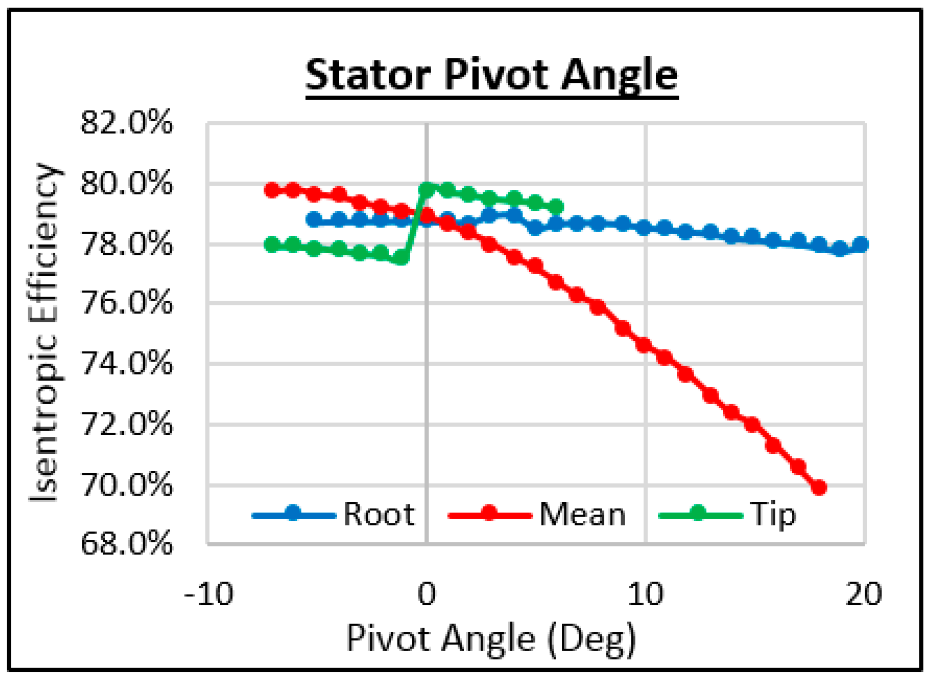
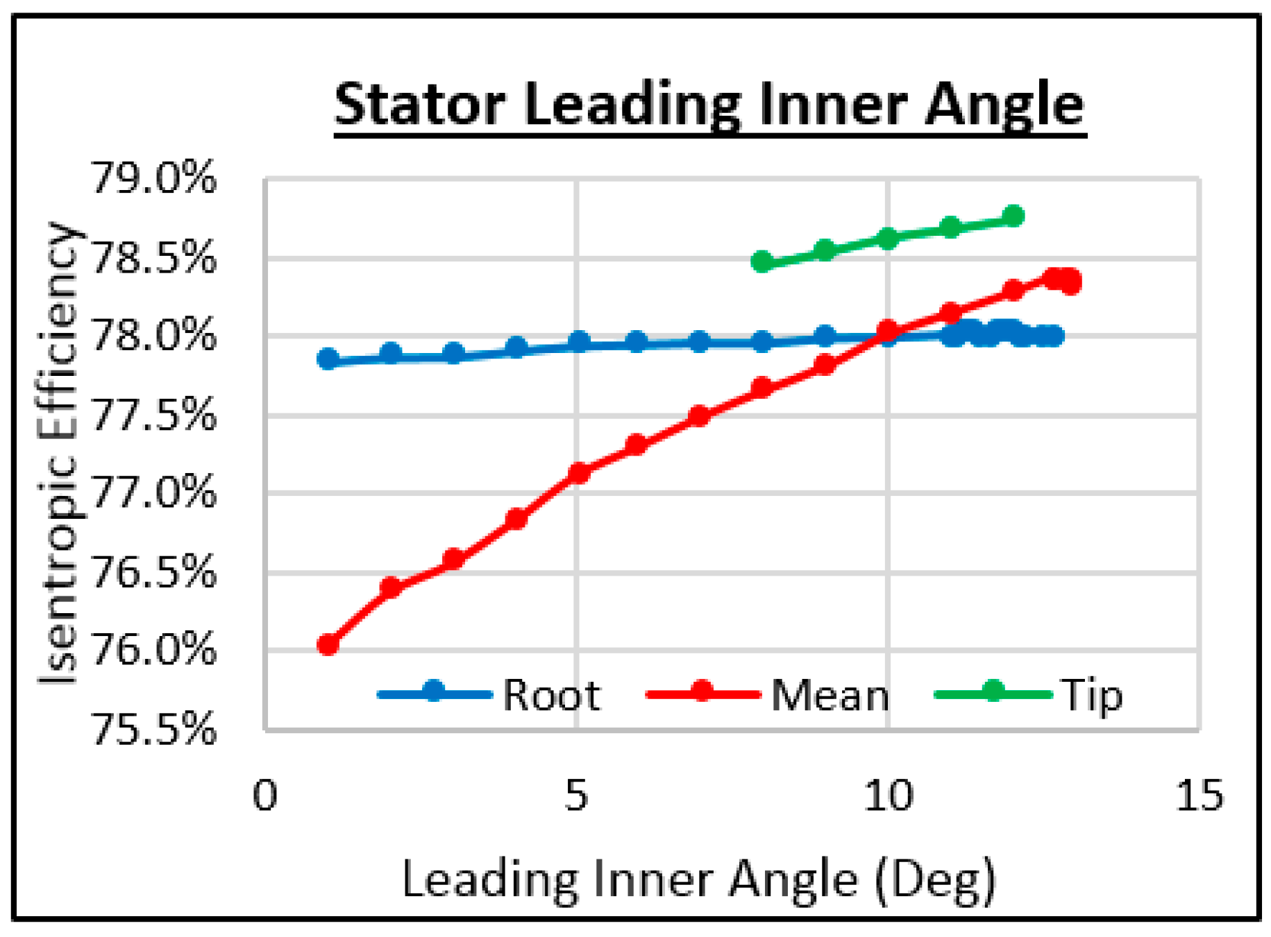
The blade pivot angle optimisation was completed before the blade angle optimisation due to the restriction that this would pose on the area-to-chord ratio. The mean pivot angle illustrated the largest variance of efficiency with a range of 10% (Figure 20). The highest efficiency was 78.89% at 3 degrees. The leading inner angle showed a similar trend with the mean profile illustrating the largest variance; this was due to the majority of the flow path entering the mid-section of the blade as opposed to the root or the tip (Figure 21). The optimum value for that angle was 12 degrees with an efficiency of 78.02%.
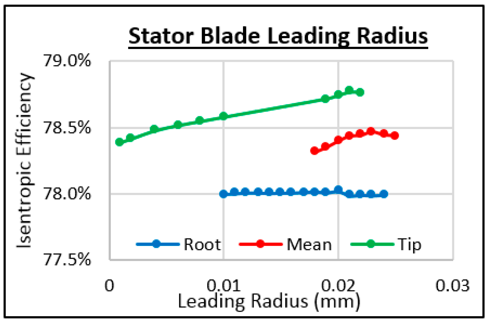
The outer angle however showed only a slight variance in isentropic efficiency indicating that the characteristics of the flow were influenced more by the inner surface which determines the direction of the flow with respect to the axial direction. Additionally a slightly larger surface area of the leading edge based on the increase in the stator’s radius improved efficiency, this would be as a result of a less abrupt flow separation at this location, reducing turbulent characteristics of the flow (Figure 22 and Figure 23).
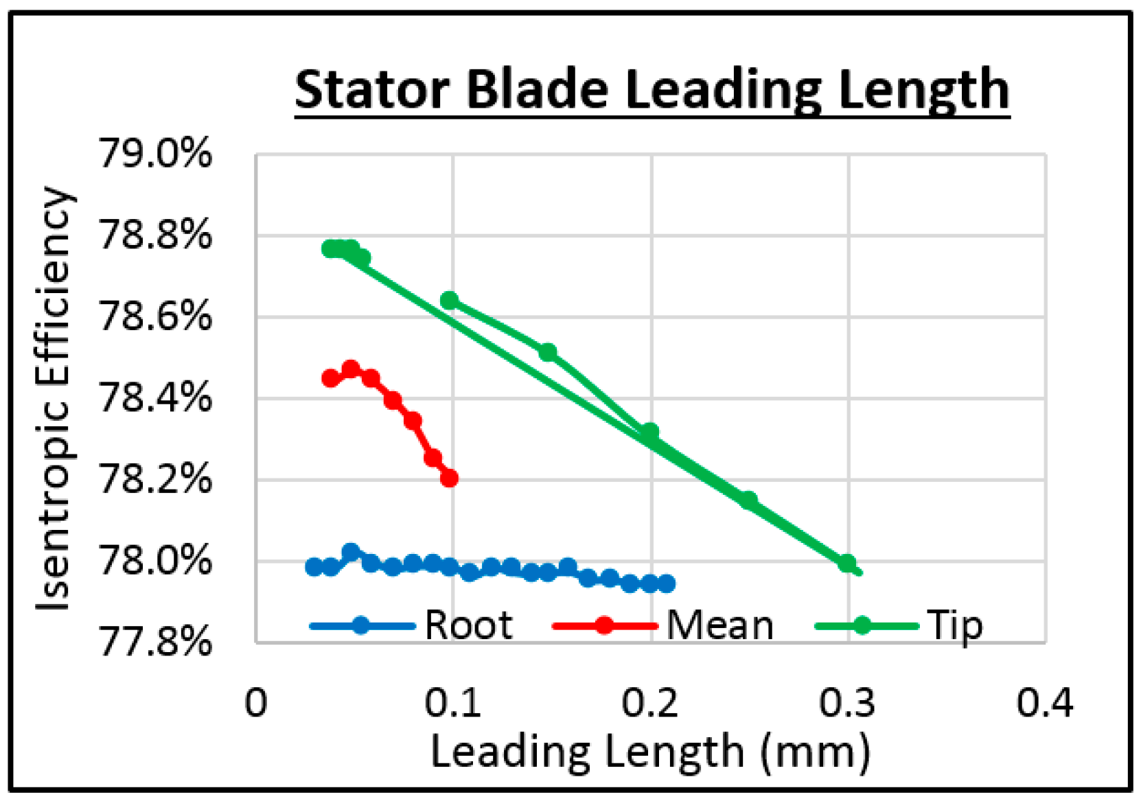
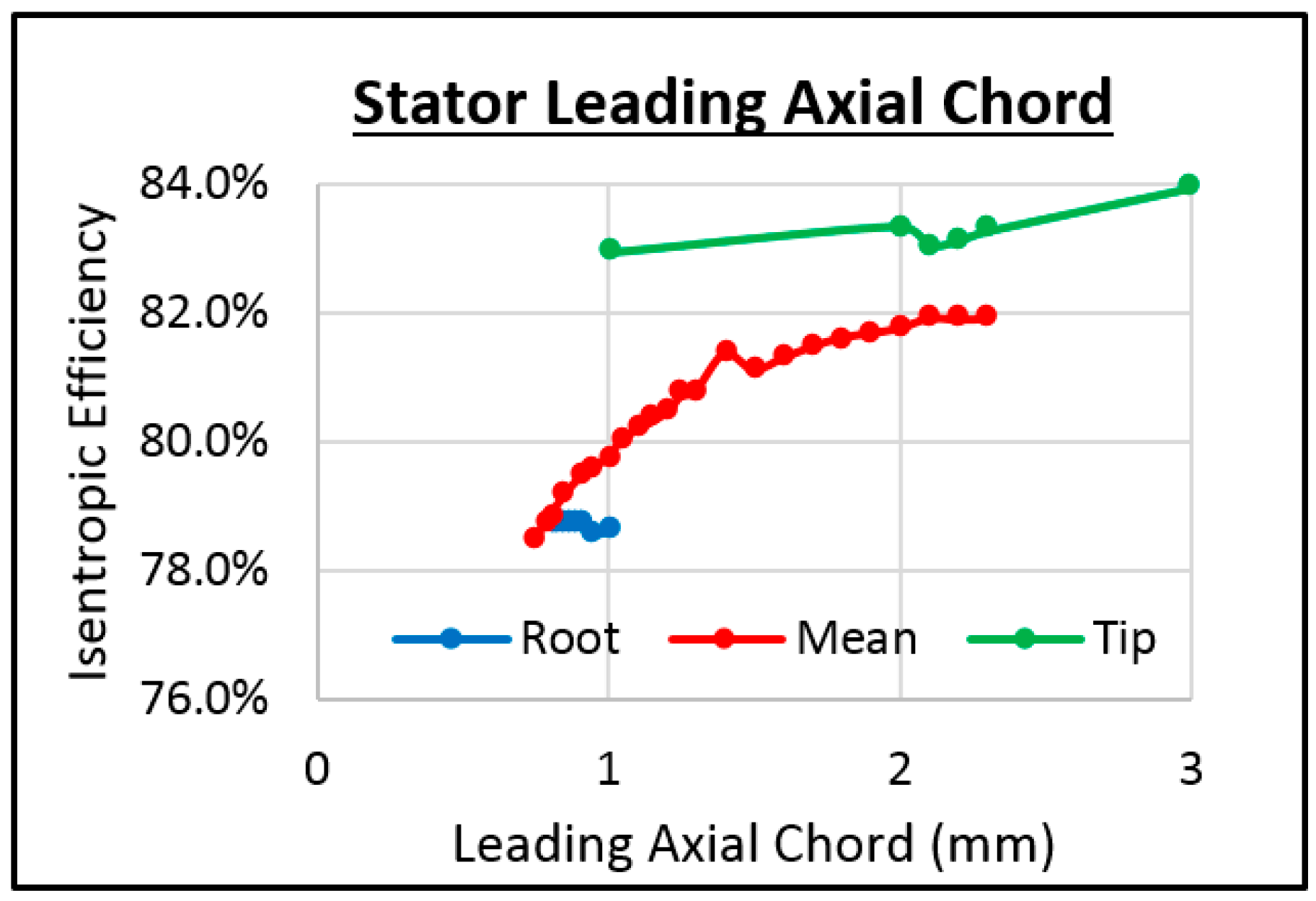
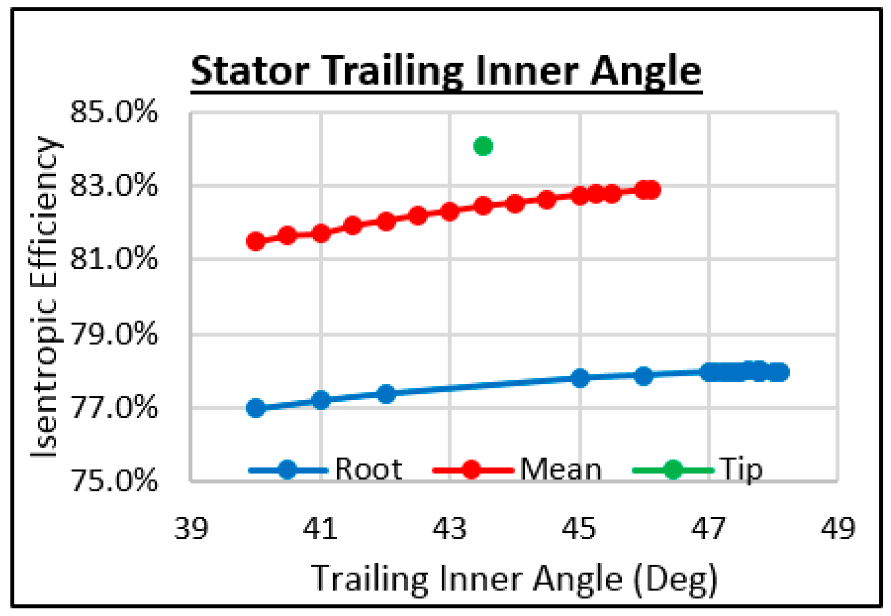
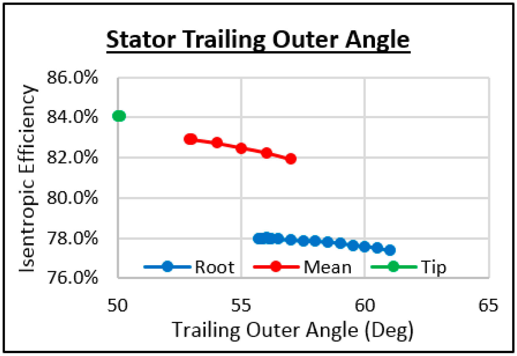
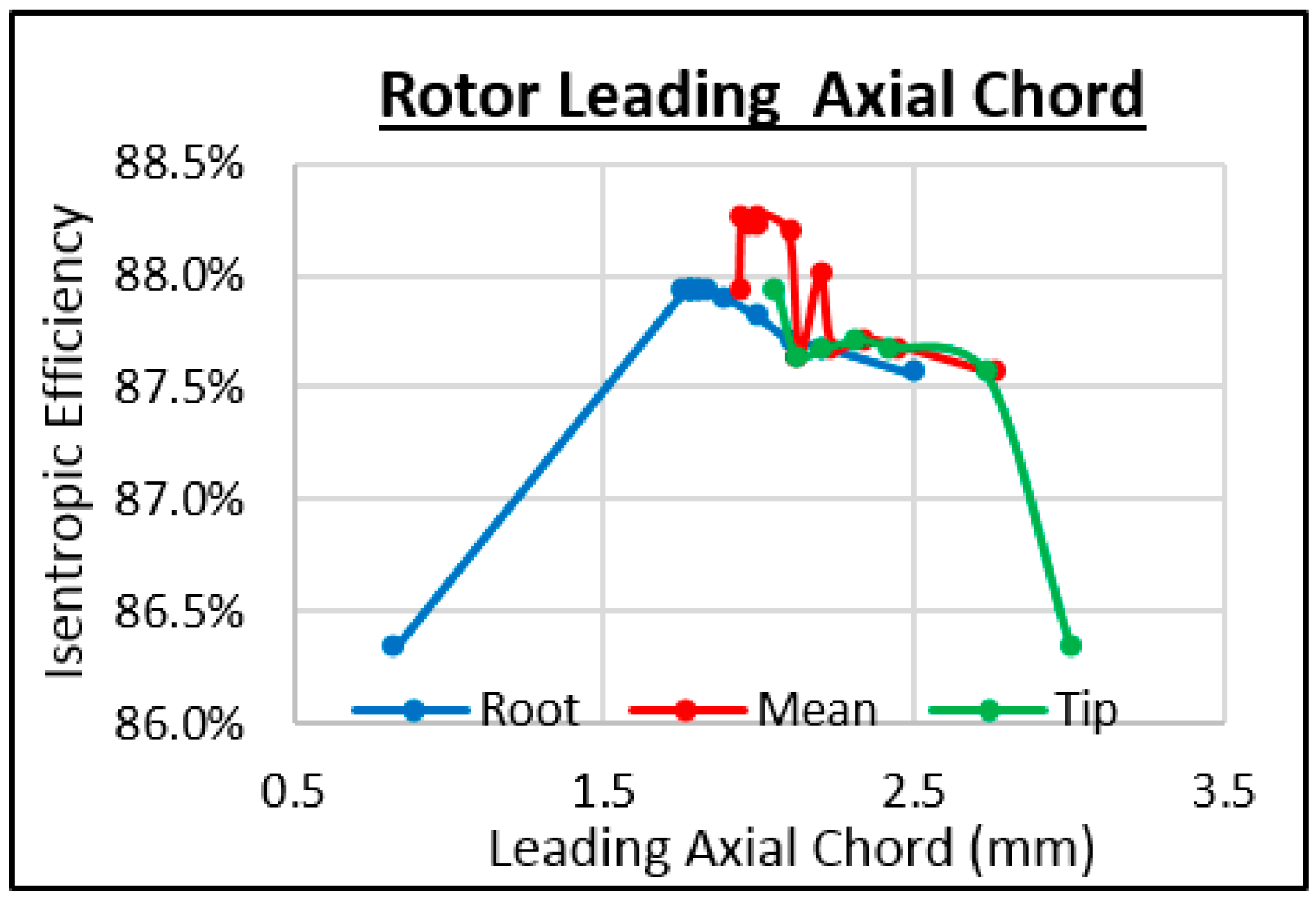
Furthermore the rate of flow separation can be translated to the leading length at both the mean and tip profile (Figure 24). Increasing this length generated a smoother transition from the leading to trailing edge section, preventing a large magnitude of flow recirculation which was previously simulated. The extension of the blade’s axial chord at both these regions also displayed an additional increase in the isentropic expansion efficiency of the axial-inflow turbine. This meant that the flow was attached to the blade for longer before entering the rotor wheel (Figure 25). Optimisation of front chord W1 at 0.84 mm provided an increase in efficiency up to 78.78%. After this every parameter which was optimised before was checked again to make sure maximum efficiency is achieved. Once all parameters were checked, rear chord W2 was optimised and efficiency was raised to 84.1% at 0.383 mm (Figure 26 and Figure 27).
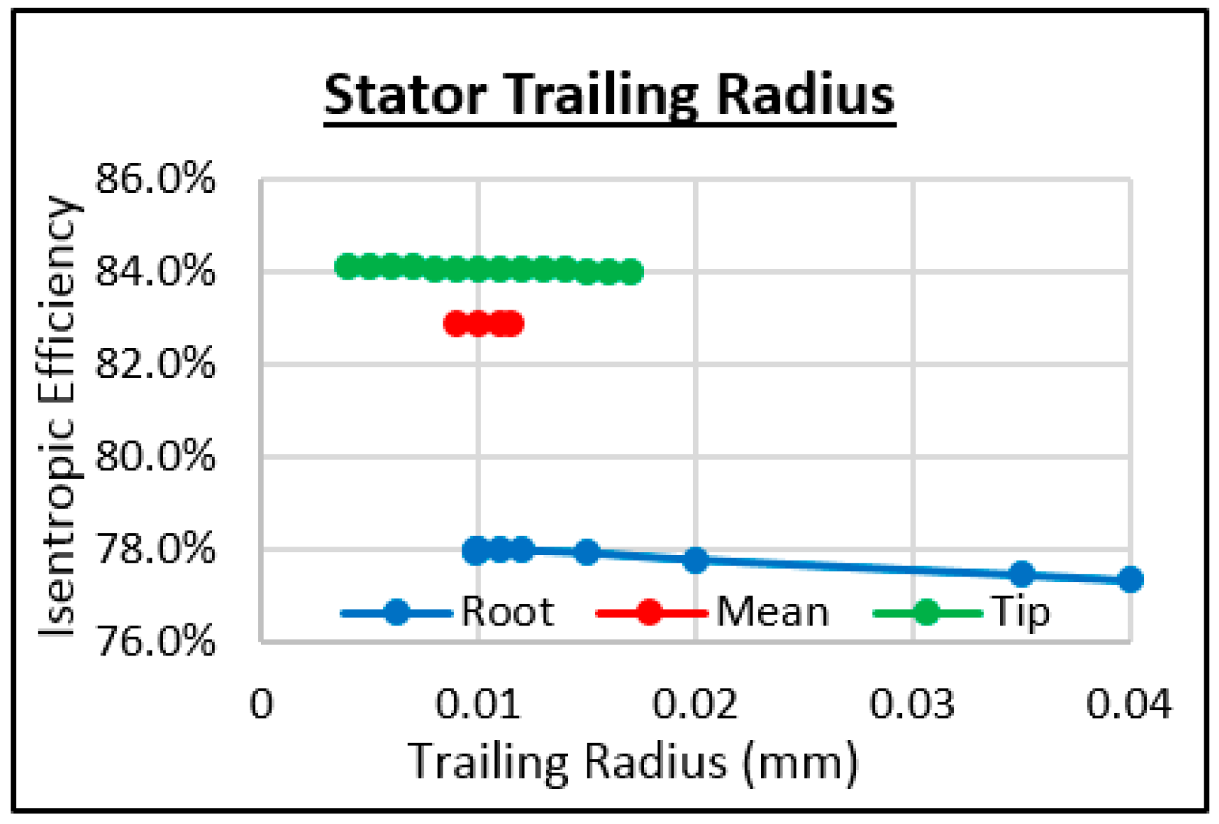
The procedure for the trailing chord was completed as a combination of all three profiles rather than individually as with the previous parameters, due to an extension of the stator mesh domain which would have impacted on the accuracy of the results if completed separately. Other than the pivot angle, the next largest improvement in efficiency was experienced by the trailing chord at 2%, directing the flow and maintaining the acceleration experienced by the fluid flow. Once all the stated parameters had been optimised, they were reviewed to update any measurements that could have been influenced by the alteration of the overall profile orientation (Figure 28 and Figure 29). Table 9, Table 10 and Table 11 provide the corresponding stator geometries.
8.4. CFD Rotor Optimisation
Each parameter of the rotor blade was optimised at all three profiles to reduce optimisation time. The axial chord was split into two sections to simplify the optimisation process, as the mesh of the rotor blade had to be moved for each new chord value to match with the stator mesh. This was done prior to optimisation of any rotor parameters.
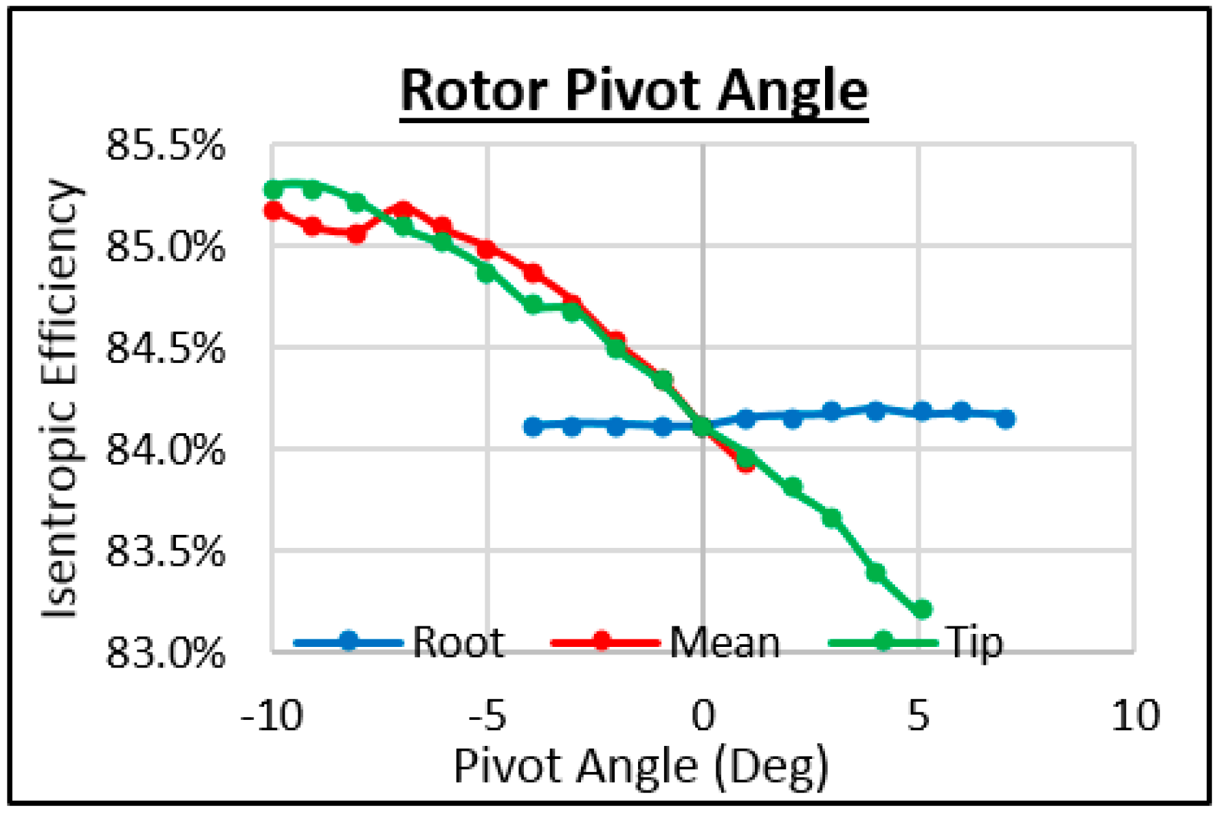
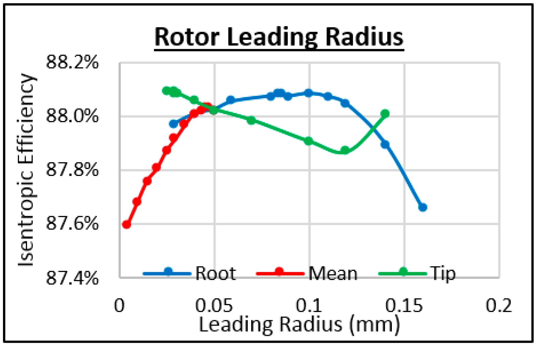
The pivot angle simulation was completed in sequence, prior to other simulations. The rotor pivot shows a similar characteristic to that of the stator but over a range of approximately 2.5% (Figure 30). The pivot angle of the profile was optimised first and the highest efficiency was 84.21% at 4 degrees. This was applied to the blade geometry to optimise the next parameter. Both angular regions of the rotor’s leading edge at the root and tip of the blade have a similar impact on the flow efficiency at an improvement of 0.4% (Figure 31 and Figure 32). The effect of the rotor leading radius maximized performance between 0.05 and 0.1 mm with the latter figure adopted (Figure 33).
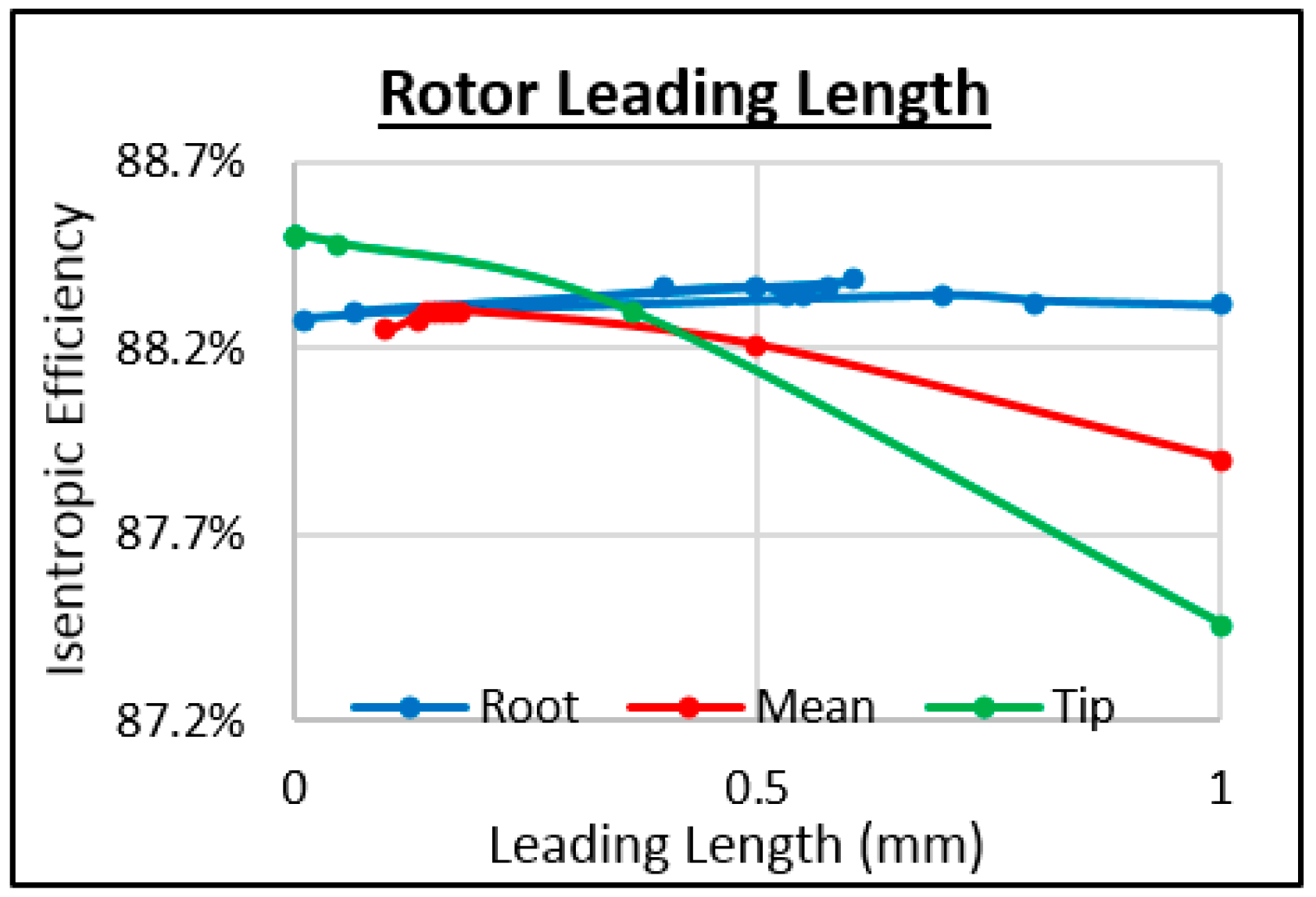
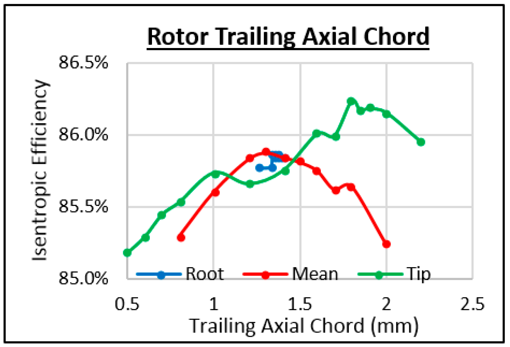
Exceeding the effect of the other simulations, the leading length (Figure 34) and axial chord (Figure 35), and indeed the trailing axial chord (Figure 36 and Figure 37) were the most important parameters during this procedure. For the leading chord this determined the positioning between the leading and trailing radiuses of the stator and rotor, respectively. Thus the effects of the magnitude of boundary layer separation could be appreciated at both regions and if incorrectly approximated, recirculation of the flow would occur at the tip surface at the root. Due to the rotation of the rotor blades, the inner angle respective to the aerofoil’s origin of rotation was transformed in order to lower the magnitude of static pressure within this region, ultimately improving the acceleration of the flow to its maximum potential (Figure 36). The outer angle on the other hand was focused on reducing the level of flow separation from the stator blades (Figure 37).
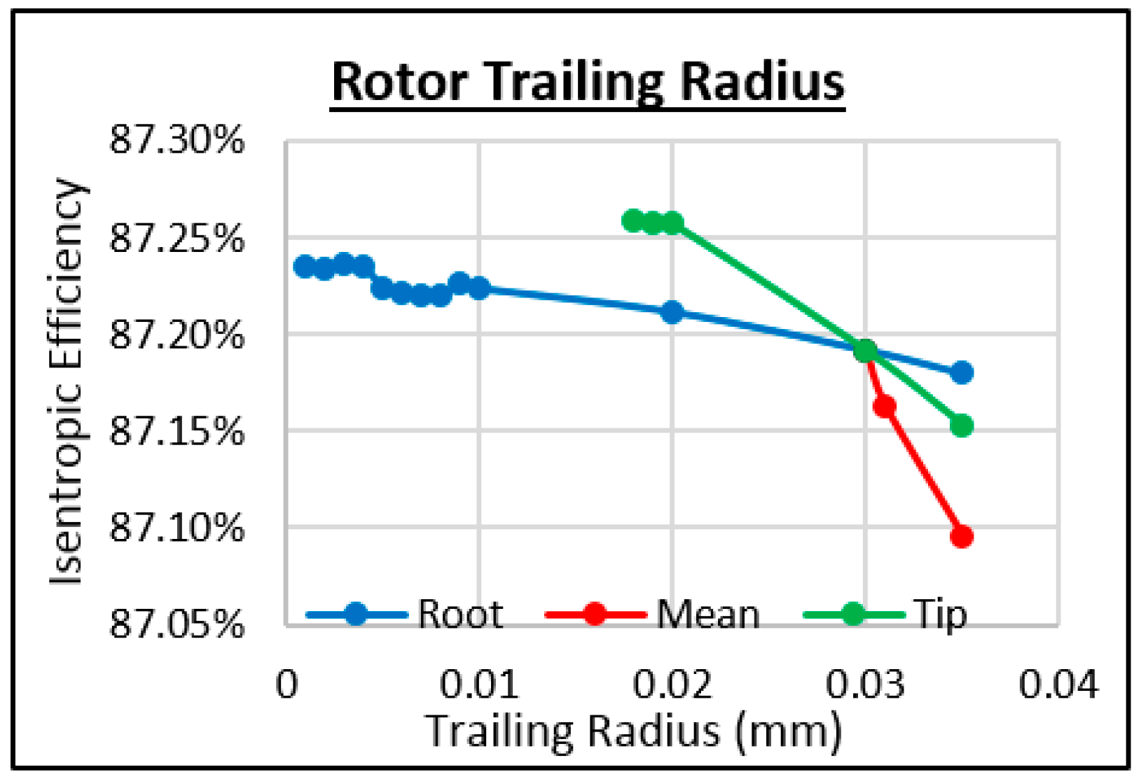
Finally, the trailing parameters were assessed as well. A trailing radius of 0.02 mm was considered to offer an acceptable compromise (Figure 38) and a trailing axial chord length of 1.5 mm was found to be the optimum length (Figure 39).
A summary of the final optimized rotor parameters is numerically provided in Table 12, Table 13 and Table 14 in terms of rotor leading and trailing lengths and root, mean and tip angles.
The final blade design through to the completion of the optimisation simulations displayed an overall total-to-total isentropic efficiency of 88.5% detailing an overall improvement of 9.8% from the initial blade design calculated, and therefore providing an input of the final design for the next stage of the simulation which was the finite element analysis for the assessment of the structural integrity of the rotor.
8.5. Variable Geometry System Optimisation
This section details the impact of changing the effective aspect ratio within the axial-inflow turbine to improve the efficiency at specific operating conditions as a result of discrete VGT operation. This aspect ratio will be analysed to provide the optimum boost pressure within this operating range. Initially, the cross-sectional area of the axial-turbine was calculated and integrated into this procedure to determine how the alteration of area would also change specific parameters illustrated at these design points (Table 15).
The main procedure investigated five separate design points corresponding to different operating points of the engine. These boundary conditions were inserted into the simulation setup and maximum turbine wheel speeds without VGT were obtained, initially, for all five design points (D.P.) (Table 16).
The detailed profiling of the VGT stator vanes and their effect on the respective efficiency of the turbine for each of the five chosen engine operating points is provided in Table 17. The regions around the optimums for each angle are shown only at increments of 1° degree.
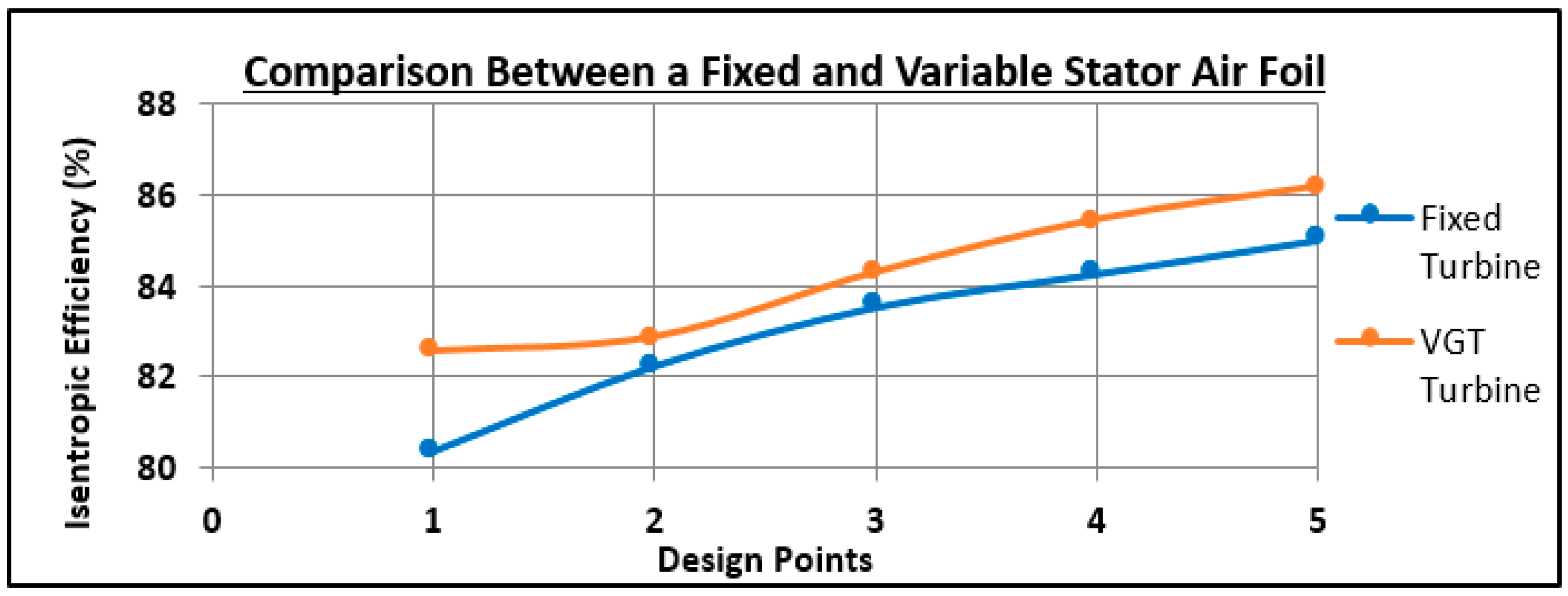
Data outside the range highlighted in Table 17 were obtained but generated a reduction in expansion efficiency. However from the analysis the maximum mass flow rate (at D.P. 5) displays an identical stator orientation to the lowest design point (D.P. 1), this was mainly due to the decrease in inlet flow velocity, characterised by the decrease in the flow temperature leading to higher density effects on the fluid. Although a frozen rotor model was used for the simulations within CFX, the fluid flow around both the stator and rotor blade profiles was taken into account. This would impact the overall efficiency of each aerofoil, allowing for an accurate comparison to be made. An additional improvement in turbine efficiency was made in each of the respective design points compared to the same axial turbine without VGT (fixed geometry or FGT configuration, Figure 40).
The most noticeable improvement of the isentropic efficiency within the turbine depicted from the computation simulations was obtained at D.P. 1 (lowest mass flow rate condition). This design point exhibited an improvement of 2.22% showing a clear advantageous approach to integrating a variable geometry system at part-load conditions. All remaining operating conditions also confirmed an improvement with an overall average of 2%. An additional investigation highlighted the ability of the VGT to accelerate the turbine to higher rotational speeds (Table 18).
While maintaining similar isentropic expansion efficiencies as the original FGT turbine, the rotor blades are able to increase in speed at all mass flow rates, thereby increasing the range at which the turbine is able to operate at its most efficient. For these specific calculations the turbine was loaded using the CFX software where the boundary conditions mentioned previously (Table 16), were inserted in order to generate an accurate representation of the turbine’s operating conditions at these five allocated design points.
9. Conclusions
The motivation behind this research project was the ability of modern heavily downsized engine and boosted engines to respond to transient engine operating point demands. Therefore for this investigation a Ford EcoBoost 1.6 L engine was selected and for which an innovative axial-inflow turbocharger turbine was designed.
The preliminary design was conducted using the researched literature of conventional axial turbines, and was based on the geometric parameters of a conventional radial turbine (GT1548). This radial turbine’s performance maps were obtained experimentally through hot-gas stand testing and allowed the boundary conditions for the axial-inflow turbine to be established. Subsequently, a velocity triangle analysis was carried out, which established the initial profile of each blade row in terms of the required blade angular geometry required, providing the basis for a 3D CFD model analysis to be carried out.
The results obtained from the CFD investigation of the axial-inflow stator and rotor blades improved the efficiency established from the preliminary design by 9.8%, through the effective alteration of blade parameters such as the pivot angle and leading and trailing angles of the blade edge. This increased the effective operating range of the axial-inflow turbine and allowed the maximum rotational velocity of the rotor established at 90,000 rpm to be increase to 102,000 rpm. The VGT operation clearly established a superiority over both the original radial turbine and the original fixed geometry axial turbine operation.
Structural analysis of the stator and rotor blades was investigated through the loading conditions established in the CFD investigation. The general levels of deformation were not considered significant and primarily focused in the trailing tip region. Where the highest deformation occurred. The modal analysis displayed no risk to the rotor failing through vibrational effects of its rotational velocity.
Finally, to determine the increase in power output now capable of the EcoBoost engine, two 1D engine models were generated using the Ricardo WAVE software. The first model represented the EcoBoost engine with the original GT1548 turbocharger and the second with the same internal combustion engine however with the Axial-Inflow VGT now attached. An equal number of simulations were run for both engine models, each at an increment of 1000 rpm. The implementation of this axial-inflow turbine provided the EcoBoost engine with the ability for an increased power output of up to 16.1 hp equating to a total power output of 186.1 hp. Therefore the combination of VGT and axial-inflow proved to provide higher engine performance in terms of power and torque (with corresponding fuel consumption reduction ramifications) compared to the baseline turbocharger turbine installed. Additionally, transient response benefits follow the implementation of such a rotor as the axial turbine rotor was a smaller device compared to the original radial turbine but the improvement in transient response and the corresponding benefits in drivability and fuel consumption reduction were outside the scope of the current work.
Acknowledgments
The author’s would like to acknowledge the contribution of the National Laboratory for Engine Turbocharging Technology (NLETT), China and its director Hua Chen in the testing of the radial turbine turbocharger.
Author Contributions
Apostolos Pesyridis conceived and designed the experiments and put forward the research concept ideas behind the project; Jordan Bradshaw and Anna Minasyan performed the experiments and analysed the data.
Conflicts of Interest
The authors declare no conflict of interest.
References
- Regulation 333/2014 Amending Regulation (EC) No 443/2009 to Define the Modalities for Reaching the 2020 Target to Reduce CO2 Emissions from New Passenger Cars OJ L 103/15, 2014. Available online: http://eur-lex.europa.eu/legal-content/EN/TXT/?uri=uriserv%3AOJ.L_.2014.103.01.0015.01.ENG (accessed on 23 March 2016).
- Pesiridis, A. Automotive Exhaust Emissions and Energy Recovery; Nova Science Publishers, Inc.: Hauppage, NY, USA, 2014. [Google Scholar]
- Reducing CO2 Emissions from Passenger Cars. 2017. Available online: http://ec.europa.eu/clima/policies/transport/vehicles/cars/index_en.htm (accessed on 6 December 2016).
- Knoema. Crude Oil Price Forecast: Long Term 2017 to 2030. 2017. Available online: https://knoema.com/yxptpab/crude-oil-price-forecast-long-term-2017-to-2030-data-and-charts (accessed on 6 December 2016).
- Zhao, H. Advanced Direct Injection Combustion Engine Technologies and Development, 1st ed.; Woodhead Publishing: Cambridge, UK, 2009; ISBN 9781845693893. [Google Scholar]
- Feneley, A.J.; Pesiridis, A.; Andwari, A.M. Variable Geometry Turbocharger Technologies for Exhaust Energy Recovery and Boosting—A Review. Renew. Sustain. Energy Rev. 2017, 71, 959–971. [Google Scholar] [CrossRef]
- Terdich, N.; Martinez-Botas, R.; Pesiridis, A.; Romagnoli, A. Mild Hybridization via Electrification of the Air System: Electrically Assisted and Variable Geometry Turbocharging Impact on an Off-Road Diesel Engine. J. Eng. Gas Turbines Power 2013, 136, 031703. [Google Scholar] [CrossRef]
- Ferrara, A.; Chen, H.; Pesiridis, A. Conceptual design of an axial turbocharger turbine. In Proceedings of the ASME TURBO EXPO 2017, GT2017-64825, Charlotte, NC, USA, 26–30 June 2017. [Google Scholar]
- Pesiridis, A.; Saccomanno, A.; Tuccillo, R.; Capobianco, A. Conceptual Design of a Variable Geometry, Axial Flow Turbocharger Turbine. In Proceedings of the 13th International Conference on Engines & Vehicles, Napoli, Italy, 10–14 September 2017. [Google Scholar]
- Cardle, R.; Giebert, D.; Mohamed, A.; Pees, S.; Oakes, M. Ultra High Efficiency Two-Stage Turbocharging System. In Proceedings of the 12th International Conference on Turbochargers and Turbocharging, Institution of Mechanical Engineers, London, UK, 17–18 May 2016. [Google Scholar]
- Stone, R. Introduction to Internal Combustion Engines, 4th ed.; Palgrave Macmillan: London, UK, 2012. [Google Scholar]
- Boyce, M.P. Axial-Flow Turbines. In Gas Turbine Engineering Handbook; Gulf Professional Publishing: Houston, TX, USA, 2011; pp. 337–350. [Google Scholar]
- Baskharone, E.A. Axial-Flow Turbines. In Principles of Turbomachinery in Air-Breathing Engines, 1st ed.; Cambridge University Press: New York, NY, USA, 2006; pp. 250–253. [Google Scholar]
- Dixon, S.L.; Hall, C. Fluid Mechanics and Thermodynamics of Turbomachinery; Butterworth-Heinemann: Oxford, UK, 2013. [Google Scholar]
Figure 1.
Velocity diagram of a turbine nozzle inlet and exit as well as as the turbine rotor exit [12].
Figure 1.
Velocity diagram of a turbine nozzle inlet and exit as well as as the turbine rotor exit [12].

Figure 2.
Stator (left) and Rotor (right) blade profiles with calculated angles.

Figure 3.
Front and side view of stator (left) and rotor (right) in TurboGrid.
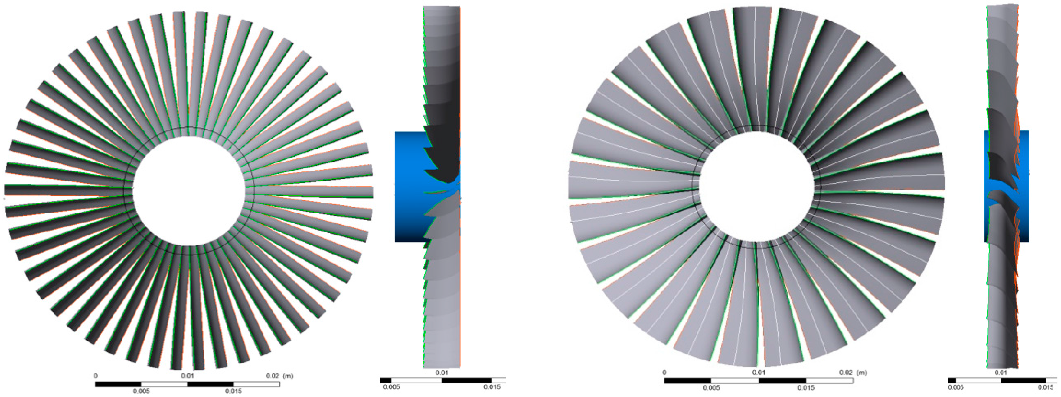
Figure 4.
Rotor blade mesh, inner walls of the domain (left) and outer walls (right).

Figure 5.
CFX setup for rotor blade and stator blade meshes.

Figure 6.
First volute design.

Figure 7.
Second volute design.
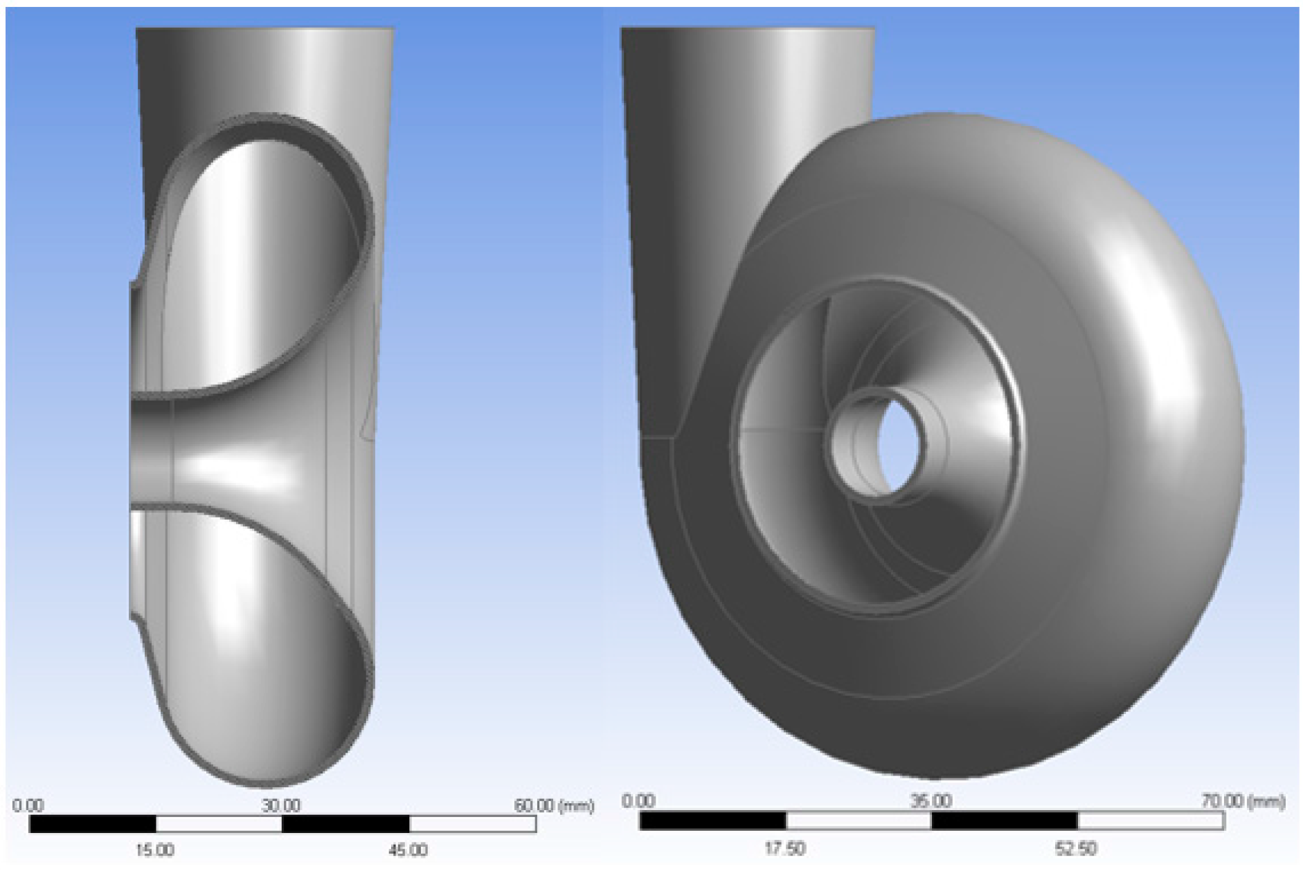
Figure 8.
Third volute design.
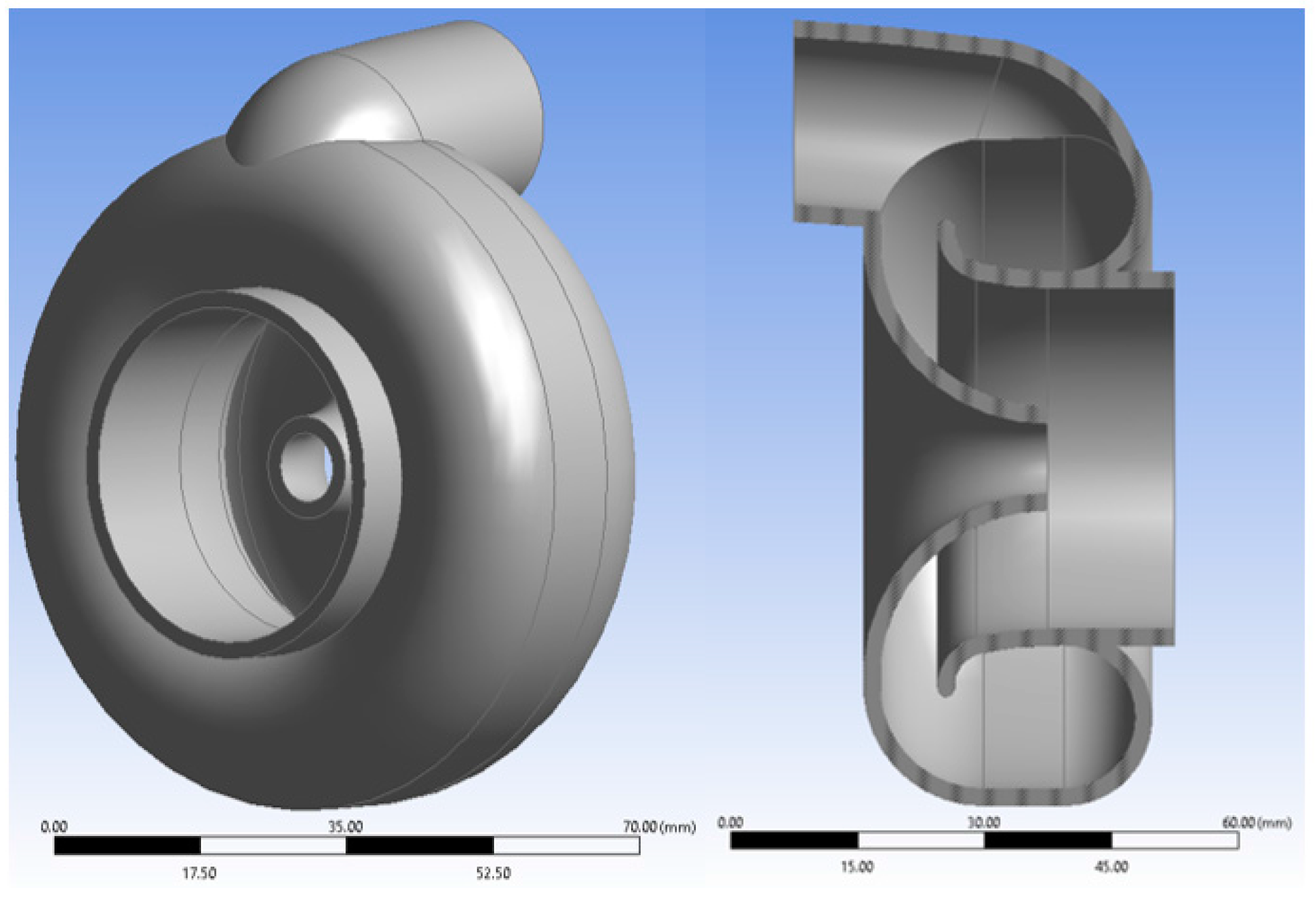
Figure 9.
Third volute design.
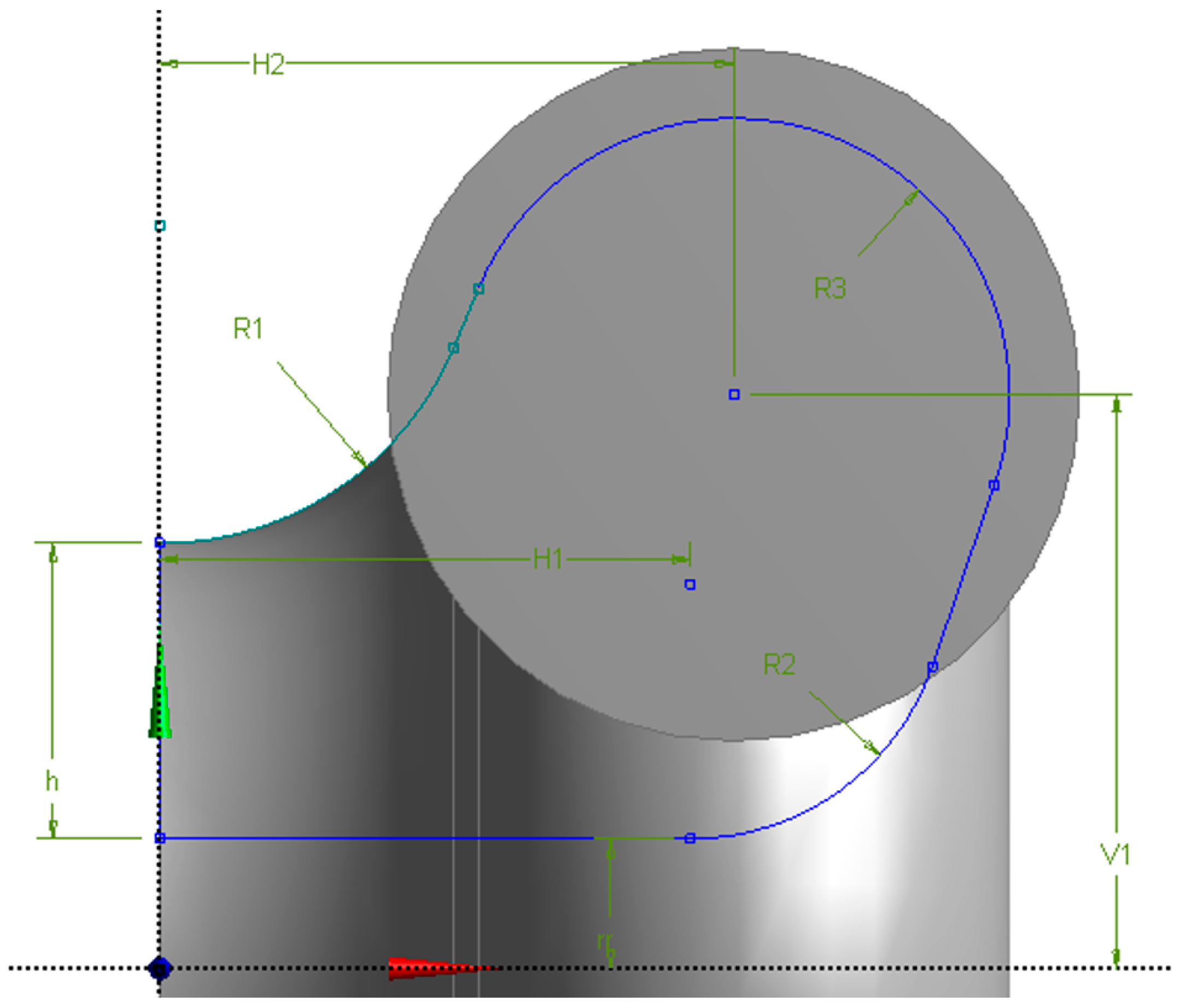
Figure 10.
Results of the first stage of the parametric volute optimisation process.
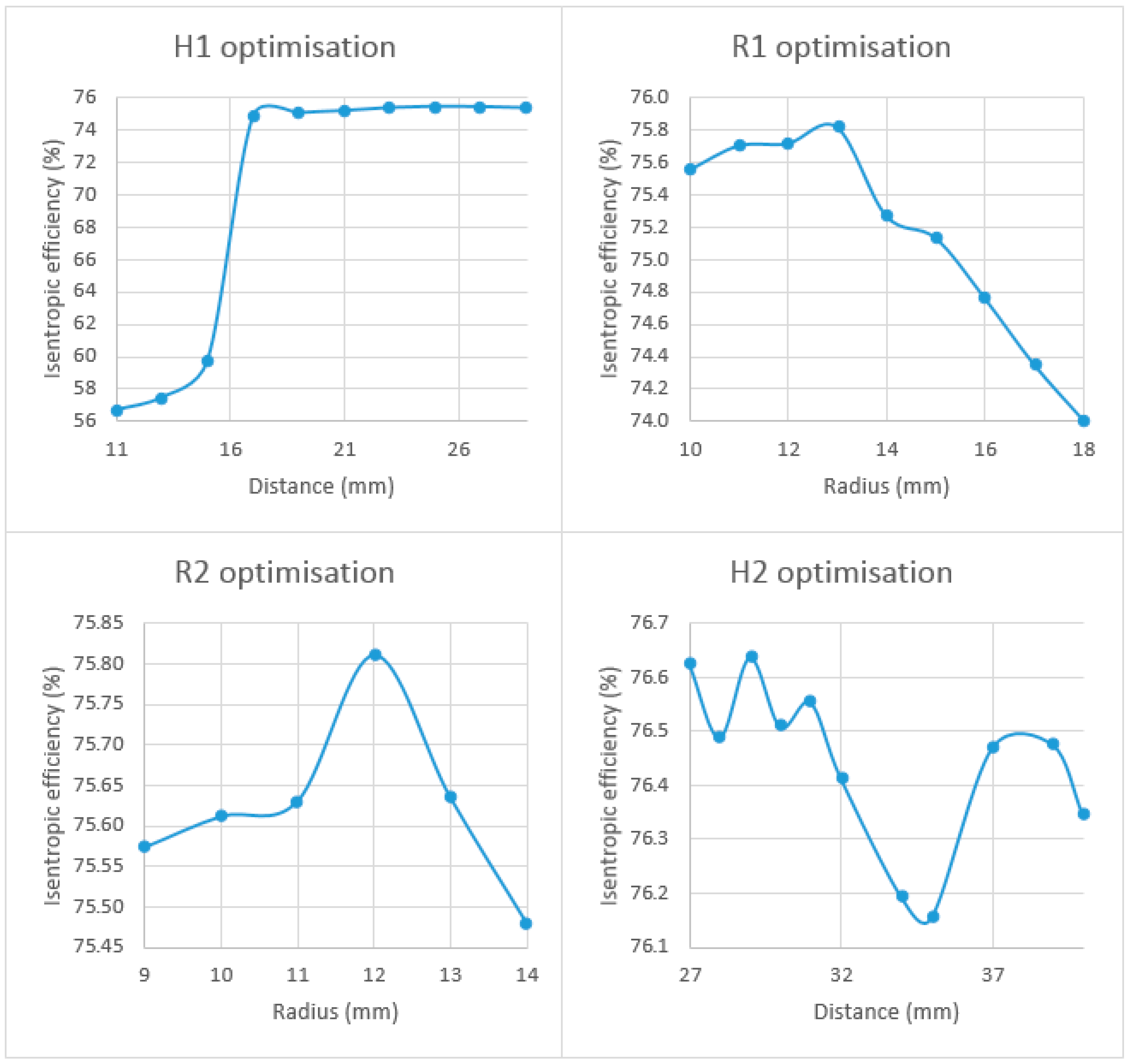
Figure 11.
Results of the second stage of the parametric volute optimisation process.
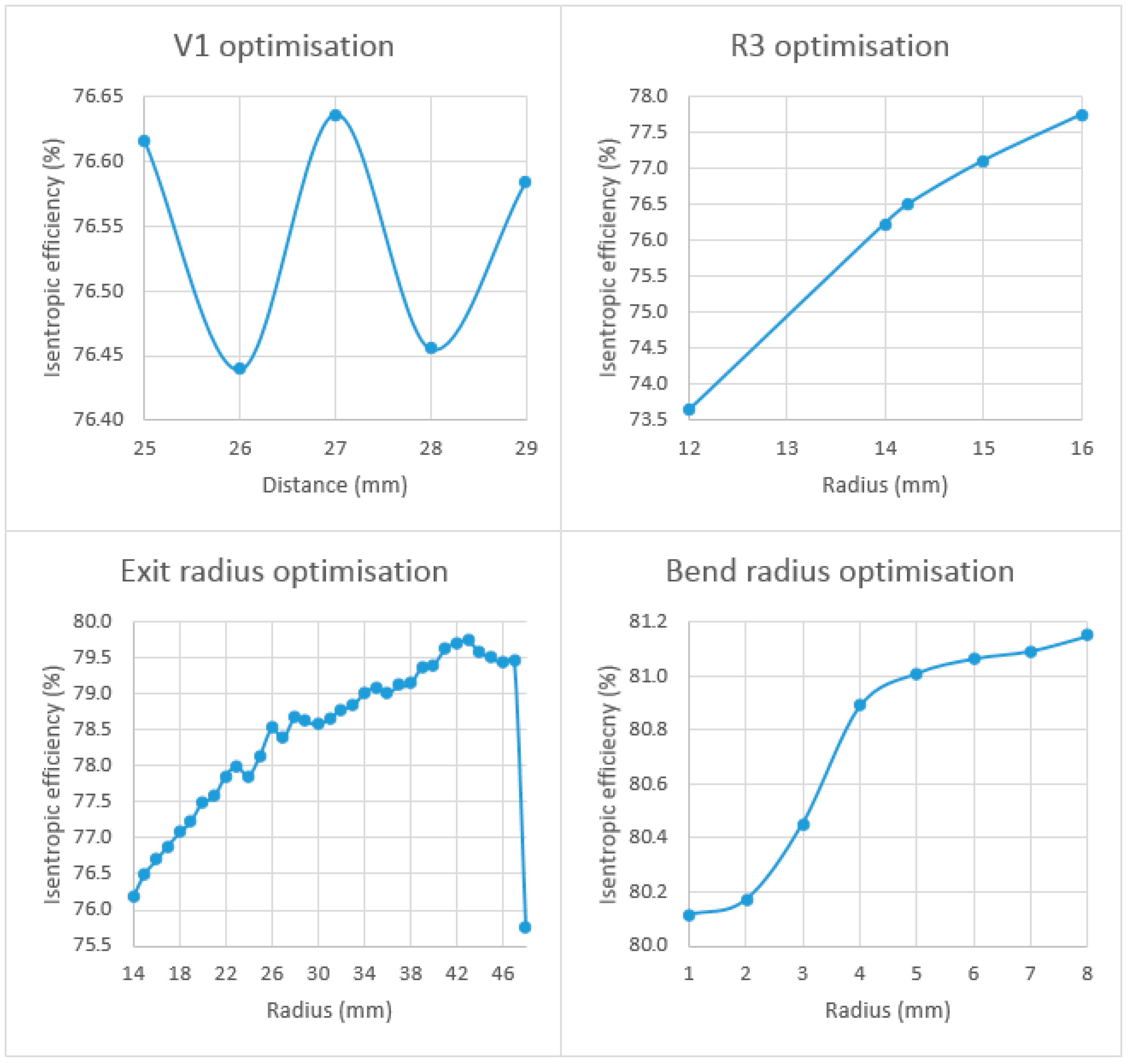
Figure 12.
Volute exit parameters.

Figure 13.
3D model of the optimised volute.

Figure 14.
Original volute, velocity streamlines.

Figure 15.
Optimised volute, velocity streamlines.
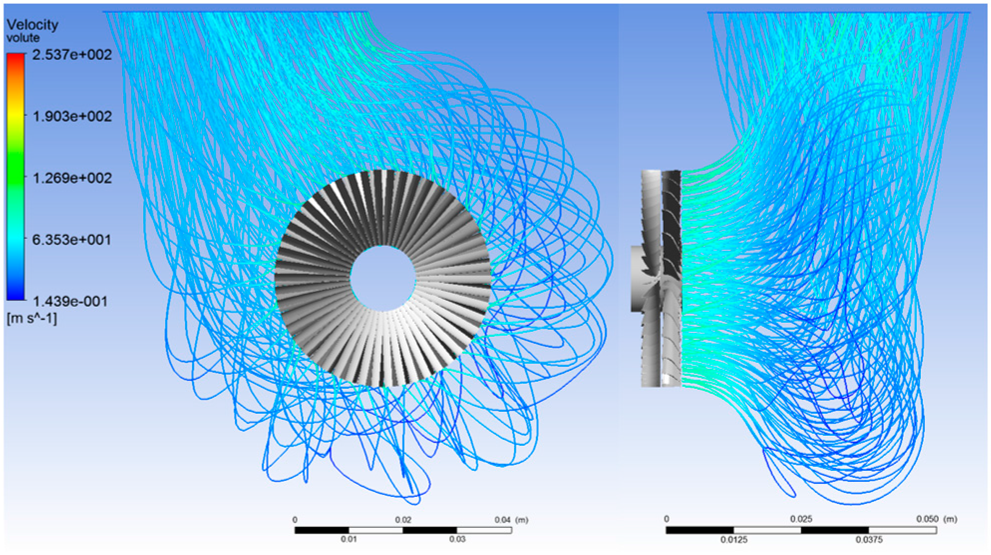
Figure 16.
Preliminary design velocity triangles at root (left) mean (centre) and tip (right).

Figure 17.
CFX results contour illustrating the translational flow path through the turbine.

Figure 18.
Data regarding the optimisation of the allocated blade numbering.
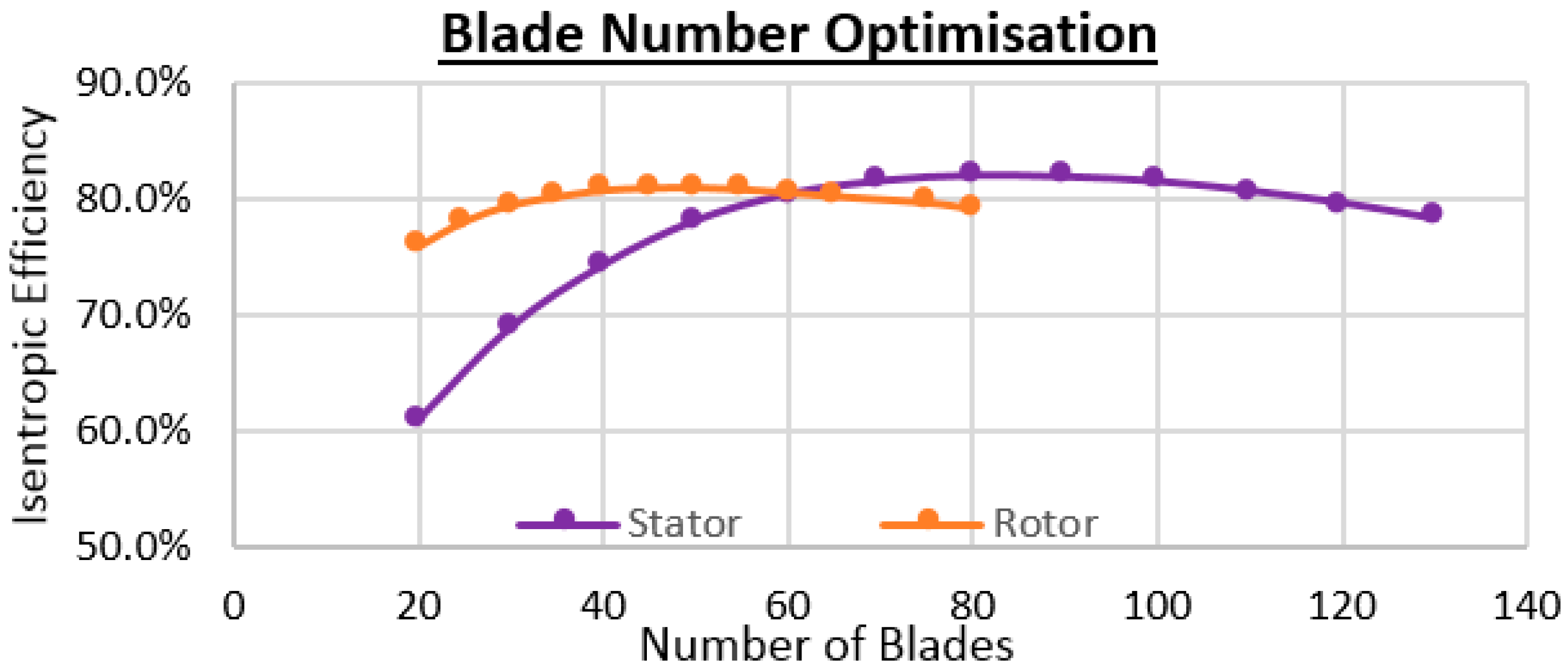
Figure 19.
Root sketch for the stator (left) and rotor (right) illustrating blade constraints.

Figure 20.
Study of the stator pivot angle.

Figure 21.
Study of the stator leading inner angle.

Figure 22.
Study of the stator leading outer angle.

Figure 23.
Study of the stator leading radius.

Figure 24.
Study of the stator leading length.

Figure 25.
Study of the stator leading axial chord.

Figure 26.
Study of the stator trailing inner angle.

Figure 27.
Study of the stator trailing outer angle.

Figure 28.
Study of the stator trailing radius.

Figure 29.
Study of the stator trailing axial chord.
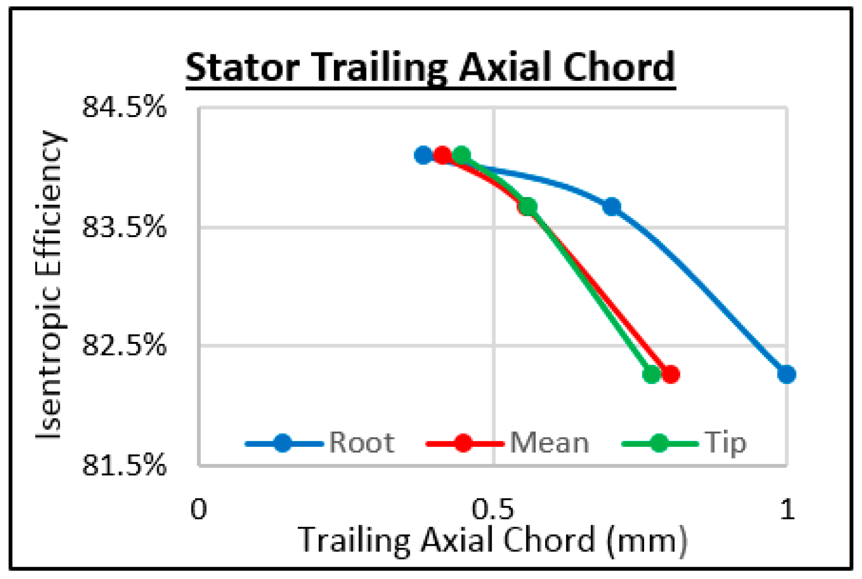
Figure 30.
Study of the rotor pivot angle.

Figure 31.
Study of the rotor leading inner angle.
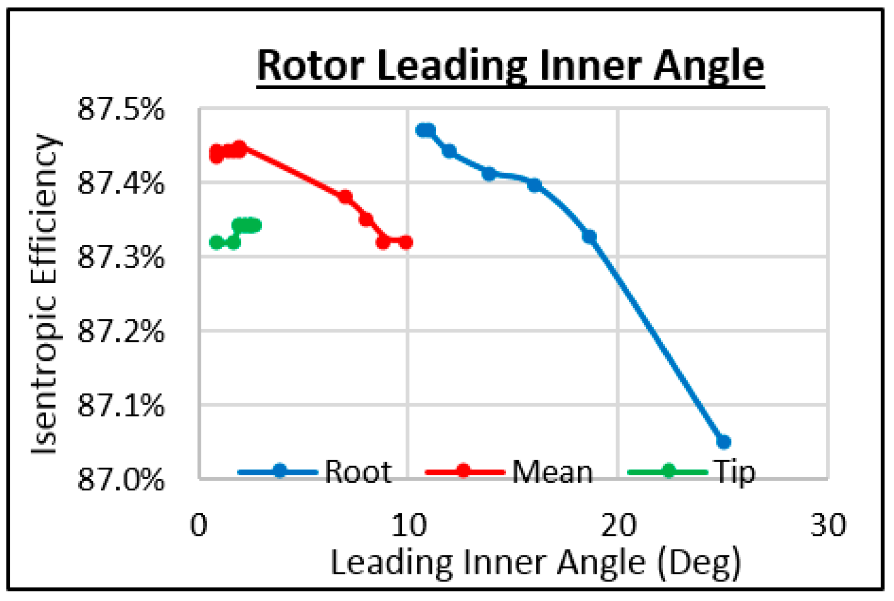
Figure 32.
Study of the rotor leading outer angle.
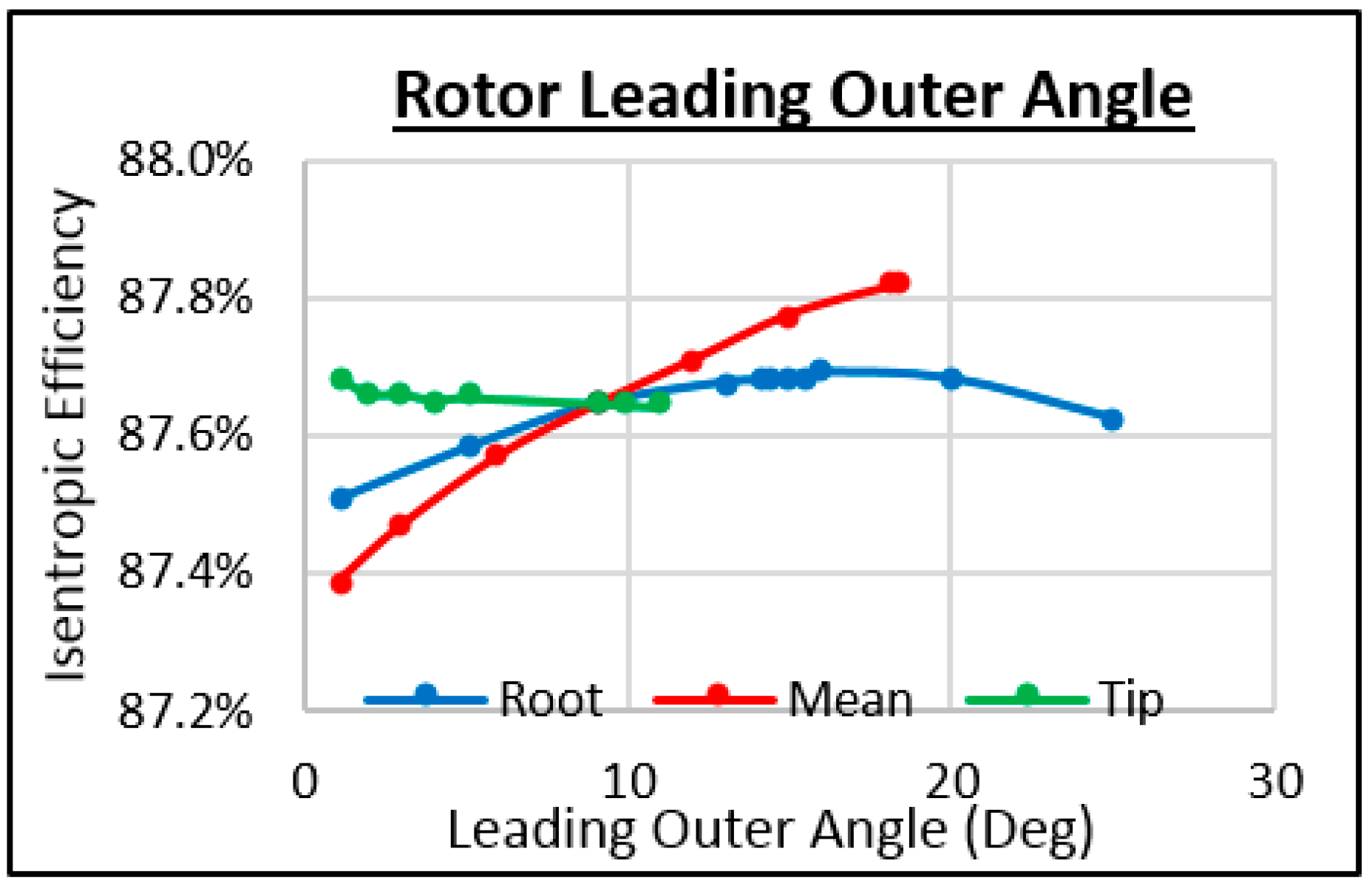
Figure 33.
Study of the rotor leading radius.

Figure 34.
Study of the rotor leading length.

Figure 35.
Study of the rotor leading axial chord.

Figure 36.
Study of the rotor trailing inner angle.
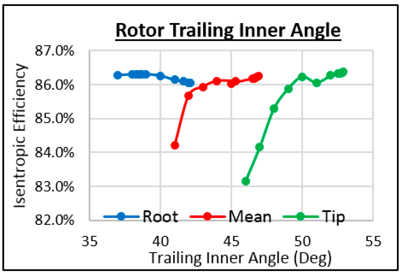
Figure 37.
Study of the rotor trailing outer angle.
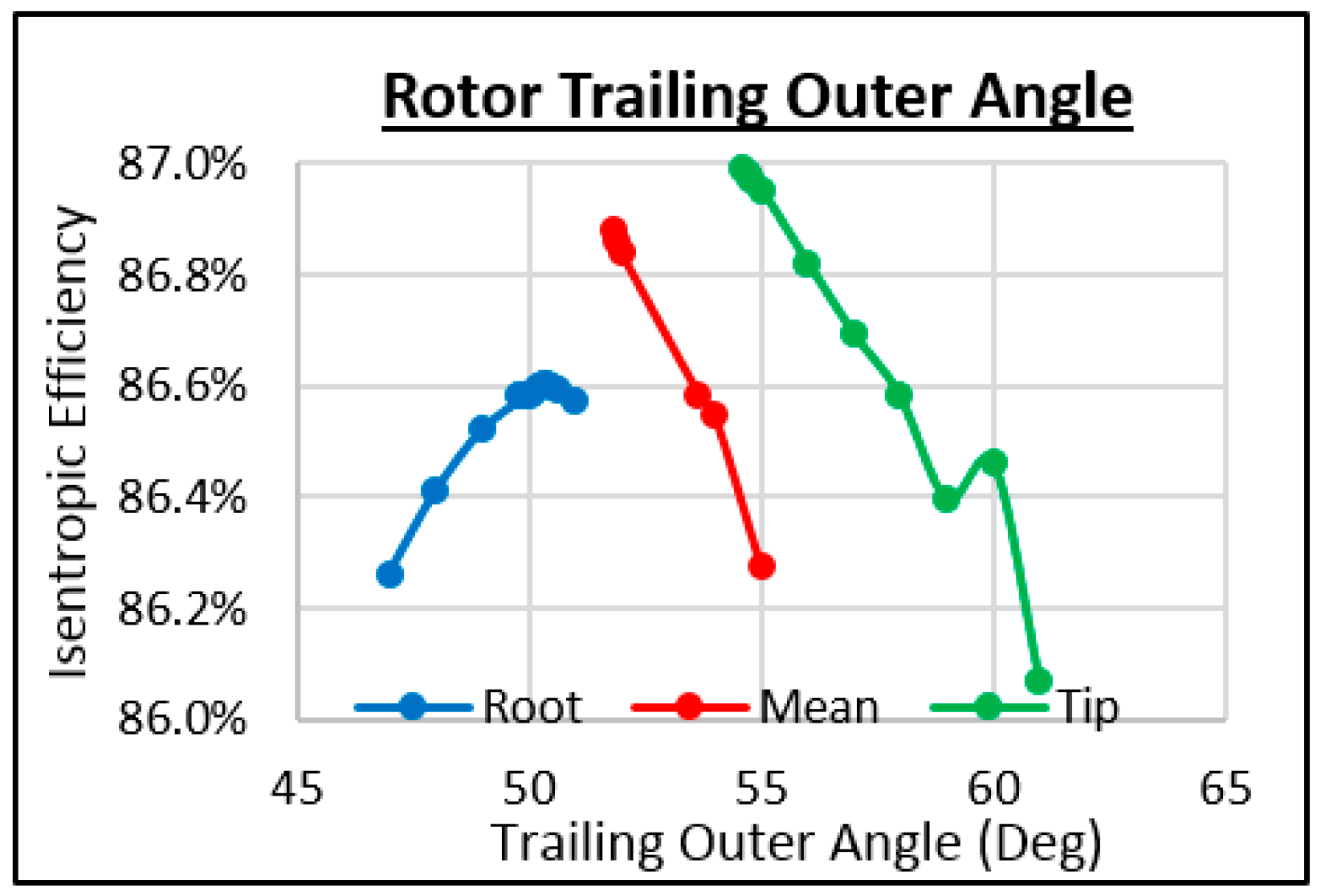
Figure 38.
Study of the rotor trailing radius.

Figure 39.
Study of the rotor’s trailing axial chord.

Figure 40.
Graphical representation of the improvement of efficiency through variable geometry.


Table 1.
Baseline turbocharger data.
| Parameter | Value |
|---|---|
| Mass flow rate (kg/s) | 0.2 |
| Inlet temperature (K) | 881 |
| Inlet pressure (kPa) | 504.554 |
| Outlet pressure (kPa) | 101.627 |
| Turbine speed (rpm) | 123,142 |
Table 2.
Assumptions for preliminary design.
| Parameter | Value |
|---|---|
| Temperature drop (K) | 60 |
| Blade speed (m/s) | 220 |
| Nozzle loss coefficient | 0.5 |
| Flow coefficient | 1.2 |
| α3 (degrees) | 10 |
Table 3.
Test data used for calculations of VGT boundary conditions.
| Inlet Parameters | Mass Flow Rate (kg/s) | ||||
|---|---|---|---|---|---|
| 0.048 | 0.079 | 0.119 | 0.153 | 0.2 | |
| Pressure (kPa) | 155.7 | 209.6 | 309.8 | 394.6 | 503.9 |
| Temperature (K) | 906 | 857 | 908 | 915 | 881 |
Table 4.
Turbine dimensions.
| Parameters of Turbine Inlet | Baseline | Axial Inflow |
|---|---|---|
| Outer radius (mm) | 0.02 | 0.02 |
| Inner radius (mm) | 0.0045 | 0.006 |
Table 5.
Preliminary design parameters for stator and rotor blades.
| Stator | Rotor | |||||
|---|---|---|---|---|---|---|
| Profile | A1 = A3 (deg) | A2 (deg) | r (mm) | B2 (deg) | B3 (deg) | r (mm) |
| root | 12.67 | 47.77 | 19.5 | 18.67 | 41.62 | 16.7 |
| mean | 10.00 | 45.27 | 21.2 | 10.00 | 45.28 | 21.2 |
| tip | 8.25 | 42.98 | 23.0 | 1.66 | 49.57 | 25.8 |
Table 6.
Measurements regarding the initial and final blade profile heights and axial chords.
| Root (mm) | Mean (mm) | Tip (mm) | Axial Chord (mm) | |
|---|---|---|---|---|
| Stator (Initial) | 19.5 | 21.25 | 23 | 1.2 |
| Stator (Final) | 6 | 13 | 20 | 1.2 |
| Rotor (Initial) | 16.7 | 21.25 | 25.8 | 3.1 |
| Rotor (Final) | 6 | 13 | 20 | 3.1 |
Table 7.
Velocity vector data collected from preliminary design.
| (m/s) | U | C2 | V2 | C3 | V3 | ||
|---|---|---|---|---|---|---|---|
| Root | 77.28 | 130.51 | 89.83 | 96.64 | 89.91 | 117.34 | 19.72 |
| Mean | 167.44 | 124.64 | 117.98 | 88.55 | 89.07 | 124.67 | 15.46 |
| Tip | 257.61 | 119.90 | 196.53 | 81.74 | 88.64 | 135.26 | 12.74 |
Table 8.
Initial angular profile of the stator and rotor blades calculated.
| Ca (m/s) | α1 (°) | α2 (°) | β2 (°) | β3 (°) | |
|---|---|---|---|---|---|
| Root | 87.72 | 12.67 | 47.77 | 18.67 | 41.62 |
| Mean | 87.72 | 10 | 45.27 | 10 | 45.28 |
| Tip | 87.72 | 8.25 | 42.98 | 1.66 | 49.57 |
Table 9.
Final parameters of the stator’s leading edge blade profiles.
| Pivot Angle (°) | Leading Inner Angle (°) | Trailing Outer Angle (°) | Trailing Radius (mm) | ||||||||
|---|---|---|---|---|---|---|---|---|---|---|---|
| R | M | T | R | M | T | R | M | T | R | M | T |
| 3 | –6 | –9 | 12 | 12.6 | 12 | 13 | 11 | 9.3 | 0.016 | 0.002 | 0.004 |
Table 10.
Final parameters of the stator’s leading length and trailing edge blade profiles.
| Leading Axial Chord (mm) | Trailing Axial Chord (mm) | ||||
|---|---|---|---|---|---|
| Root | Mean | Tip | Root | Mean | Tip |
| 0.84 | 2.10 | 3.00 | 0.383 | 0.414 | 0.447 |
Table 11.
Final parameters of the stator’s leading and trailing axial chords.
| Leading Length (mm) | Leading Inner Angle (°) | Trailing Outer Angle (°) | Trailing Radius (mm) | ||||||||
|---|---|---|---|---|---|---|---|---|---|---|---|
| R | M | T | R | M | T | R | M | T | R | M | T |
| 0.06 | 0.7 | 1.16 | 48 | 46 | 43.5 | 56 | 53 | 50 | 0.01 | 0.009 | 0.004 |
Table 12.
Final parameters of the rotor’s leading edge blade profiles.
| Pivot Angle (°) | Leading Inner Angle (°) | Trailing Outer Angle (°) | Trailing Radius (mm) | ||||||||
|---|---|---|---|---|---|---|---|---|---|---|---|
| R | M | T | R | M | T | R | M | T | R | M | T |
| 4 | –3 | –9 | 10.8 | 2 | 2.5 | 16 | 18.5 | 1 | 0.09 | 0.045 | 0.03 |
Table 13.
Final parameters of the rotor’s leading length and trailing edge blade profiles.
| Leading Length (mm) | Trailing Inner Angle (°) | Trailing Outer Angle (°) | Trailing Radius (mm) | ||||||||
|---|---|---|---|---|---|---|---|---|---|---|---|
| R | M | T | R | M | T | R | M | T | R | M | T |
| 0.55 | 0.15 | 0.001 | 38.5 | 46.9 | 52.9 | 50.4 | 51.8 | 555 | 0.0025 | 0.025 | 0.018 |
Table 14.
Final parameters of the rotor, leading and trailing axial chords.
| Leading Axial Chord (mm) | Trailing Axial Chord (mm) | ||||
|---|---|---|---|---|---|
| Root | Mean | Tip | Root | Mean | Tip |
| 1.8 | 2.0 | 2.33 | 1.365 | 1.3 | 1.8 |
Table 15.
Data comparison of the cross-sectional area of the GT1548 and axial-inflow turbines.
| GT1548 Radial | Axial-Inflow | |
|---|---|---|
| Outer Diameter Frontal Area (mm2) | 1.257 × 10⁻³ | 1.257 × 10⁻³ |
| Shaft Frontal Area (mm2) | 0.064 × 10⁻³ | 0.113 × 10⁻³ |
| Cross-Sectional Area (mm2) | 1.193 × 10⁻³ | 1.144 × 10⁻³ |
Table 16.
Inlet boundary conditions with maximum turbine speeds.
| Design Point | D.P. 1 | D.P. 2 | D.P. 3 | D.P. 4 | D.P. 5 |
|---|---|---|---|---|---|
| Speed without VGT (rpm) | 52,000 | 71,000 | 85,000 | 89,000 | 90,000 |
| Mass flow rate (kg/s) | 0.048 | 0.079 | 0.119 | 0.153 | 0.200 |
| inlet temperature (K) | 905.5 | 856.7 | 908.3 | 915.2 | 880.7 |
| inlet velocity (m/s) | 70.05 | 81.05 | 87.55 | 89.07 | 87.72 |
Table 17.
VGT analysis of each mass flow rate against the respective change in the stator profile.
| Root Angle | Mean Angle | Tip Angle | D.P. 1 Efficiency | D.P. 2 Efficiency | D.P. 3 Efficiency | D.P. 4 Efficiency | D.P. 5 Efficiency |
|---|---|---|---|---|---|---|---|
| 9° | 0° | −3° | 82.56% | 82.87% | 84.22% | 84.68% | 86.19% |
| 8° | −1° | −4° | 82.39% | 82.78% | 84.18% | 84.69% | 86.07% |
| 7° | −2° | −5° | 82.28% | 82.87% | 84.29% | 85.46% | 85.82% |
| 6° | −3° | −6° | 81.92% | 82.65% | 84.19% | 85.12% | 85.61% |
| 5° | −4° | −7° | 81.73% | 82.42% | 83.87% | 84.87% | 85.46% |
| 4° | −5° | −8° | 81.34% | 82.21% | 83.69% | 84.49% | 85.32% |
| 3° | −6° | −9° | 80.33% | 82.22% | 83.52% | 84.26% | 85.01% |
Table 18.
Comparison between the original FGT rotational speed and the rotational speed obtained with VGT.
Table 18.
Comparison between the original FGT rotational speed and the rotational speed obtained with VGT.
| D.P. 1 | D.P. 2 | D.P. 3 | D.P. 4 | D.P. 5 | |
|---|---|---|---|---|---|
| Original FGT (rpm) | 52,000 | 71,000 | 85,000 | 89,000 | 90,000 |
| VGT (rpm) | 57,000 | 75,000 | 90,000 | 97,000 | 102,000 |
© 2018 by the authors. Licensee MDPI, Basel, Switzerland. This article is an open access article distributed under the terms and conditions of the Creative Commons Attribution (CC BY) license (http://creativecommons.org/licenses/by/4.0/).
Share and Cite
MDPI and ACS Style
Minasyan, A.; Bradshaw, J.; Pesyridis, A. Design and Performance Evaluation of an Axial Inflow Turbocharger Turbine. Energies 2018, 11, 278. https://doi.org/10.3390/en11020278
AMA Style
Minasyan A, Bradshaw J, Pesyridis A. Design and Performance Evaluation of an Axial Inflow Turbocharger Turbine. Energies. 2018; 11(2):278. https://doi.org/10.3390/en11020278
Chicago/Turabian StyleMinasyan, Anna, Jordan Bradshaw, and Apostolos Pesyridis. 2018. "Design and Performance Evaluation of an Axial Inflow Turbocharger Turbine" Energies 11, no. 2: 278. https://doi.org/10.3390/en11020278
Note that from the first issue of 2016, this journal uses article numbers instead of page numbers. See further details here.