Application of H∞ Robust Control on a Scaled Offshore Oil and Gas De-Oiling Facility


Department of Energy Technology, Aalborg University, Esbjerg Campus, Niels Bohrs Vej 8, 6700 Esbjerg, Denmark
*
Author to whom correspondence should be addressed.
Energies 2018, 11(2), 287; https://doi.org/10.3390/en11020287
Submission received: 21 December 2017
/
Revised: 13 January 2018
/
Accepted: 22 January 2018
/
Published: 24 January 2018
(This article belongs to the Section L: Energy Sources)
Abstract
:The offshore de-oiling process is a vital part of current oil recovery, as it separates the profitable oil from water and ensures that the discharged water contains as little of the polluting oil as possible. With the passage of time, there is an increase in the water fraction in reservoirs that adds to the strain put on these facilities, and thus larger quantities of oil are being discharged into the oceans, which has in many studies been linked to negative effects on marine life. In many cases, such installations are controlled using non-cooperative single objective controllers which are inefficient in handling fluctuating inflows or complicated operating conditions. This work introduces a model-based robust H control solution that handles the entire de-oiling system and improves the system’s robustness towards fluctuating flow thereby improving the oil recovery and reducing the environmental impacts of the discharge. The robust H control solution was compared to a benchmark Proportional-Integral-Derivative (PID) control solution and evaluated through simulation and experiments performed on a pilot plant. This study found that the robust H control solution greatly improved the performance of the de-oiling process.
1. Introduction
Since the late 1960s, the North Sea has been home to a booming Oil and Gas industry and has provided substantial quantities of petroleum products [1]. Reservoirs that are located beneath the ocean seabed were initially pressurized with high concentrations of oil and gas and relatively small amounts of water. The long period of oil exploration has had its toll on the reservoirs, wherein natural water leakage into the reservoirs and water re-injection have changed the balance of oil, gas and water concentrations [2]. Presently, the fluids pumped from the reservoirs has in many cases a water fraction, and, due to conveyance costs, the water must be separated from the product on the offshore facilities [3,4,5]. In the Danish sector, the water fraction has increased by over the period of 2005 to 2015 resulting in an increasing strain on the separation facilities who must adhere to discharge regulations [6]. The current regulation for the Oil in Water (OiW) concentration in the discharge into the North Sea is 30 mg/L [7]. In most cases, the OiW discharges from the North Sea operators can be maintained far below the required limits; for example, the average OiW concentration for the year 2011 in the Danish sector of the North Sea was 4.8 mg/L [8]. The limit is exceeded occasionally, for example, in 2008, there were 25 instances where the monthly average limit was exceeded in the Danish sector of the North Sea, although the number of such instances has fallen drastically and the limit was exceeded just once in 2012 [8]. It is, however, vital to keep in mind that the OiW in the discharge is measured offline using a Gas Chromatography with Flame-Ionization Detection (GC-FID) instrument, where at least two samples per day in accordance with the OSPAR Convention’s OSPAR reference method (ISO 9377-2 GC-FID) are taken [9,10], and that above exceptions is a monthly average. Thus, statistically, the number of discharges that exceeded the limits is potentially greater and could be very high OiW concentrations at times. Another important factor is not merely the oil discharge concentration but the total bulk of oil discharged, which is increasing due to the increase in the total liquid volume that is produced. In 2015, the total mass of oil discharged into the North Sea was 193 tonnes, whereas the limit set by the Danish Government is 202 tonnes per annum [11]. It is thus of high importance to continually improve the de-oiling facilities and their operation and control, to have a steady discharge and keep the OiW concentration below the required limit and approach a zero discharge. This article focuses on improving the performance of a de-oiling facility using a novel control solution.
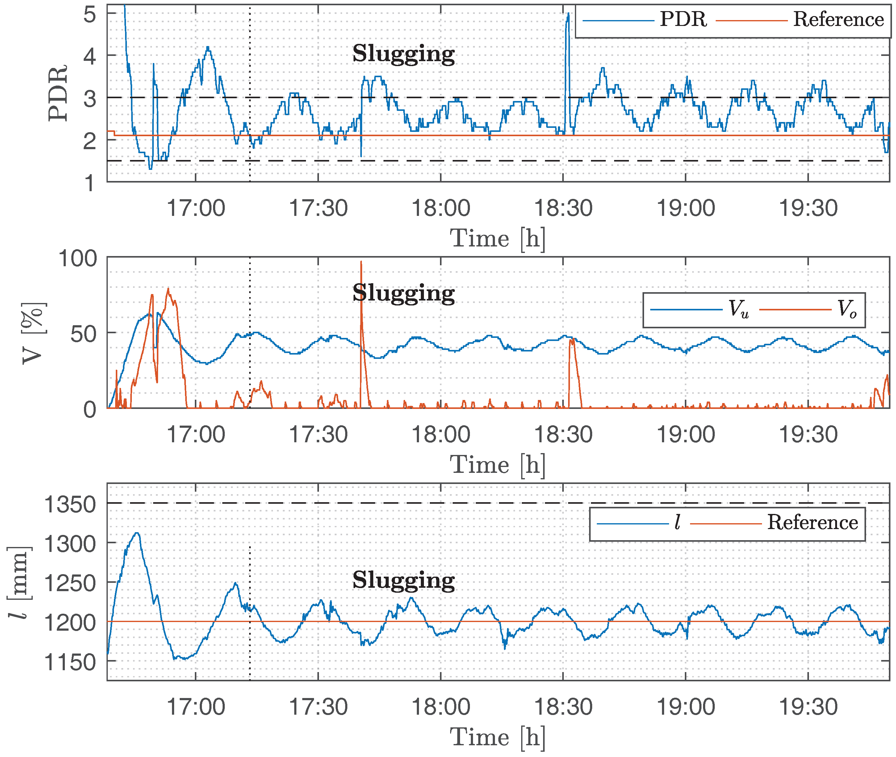
The most common units of a de-oiling unit process are a three-phase gravity separator followed by a de-oiling hydrocyclone separator [12,13,14,15,16,17]. The control of such a conventional de-oiling system is performed by two Proportional-Integral-Derivative (PID) controllers that control the level in the gravity separator and the pressure drop ratio (PDR) across the hydrocyclone. A Piping and Instrumentation Diagram (P&ID) of the de-oiling system that is considered in this study can be seen in Figure 1. In previous work, it was shown that such a system is sensitive towards fluctuating inlet flow rate [15,18,19,20], which is a re-occurring phenomenon in such installations and in most occasions it is caused by slugging flow regime in the upstream pipeline system [21,22,23]. An investigation of the offshore data, as shown in Figure 2, shows a typical performance of a conventional de-oiling controller, consisting of two individual PID controllers, a level and a PDR controller, as shown in Figure 1, during a fluctuating inlet flow rate.
Here, the fluctuations are directly transmitted into an actuation of the underflow valve which aims a maintaining the level, and by doing so disrupts the PDR value, which in many cases exceeds its boundary, as indicated in Figure 2 by the horizontal dashed lines. Due to the relatively larger physical size of the underflow valve and the physical coupling in the system, it dominates the overflow valve that is used to control the PDR [24]. This leads to the overflow valve chattering at almost fully closed position for long periods of time, which results in excess oil being sent through the underflow along with the water, and if this is not recirculated through the de-oiling system, the oil will be discharged into the ocean. In the opposite case when the overflow valve is fully open, excess water will be sent through the overflow, which, again, necessitates recirculation in order to purify the overflow. It was shown in [14,25] that a hydrocyclone operates at a high efficiency as long as the pressure drop ratio (PDR) and the inlet flow rate to the hydrocyclone are kept within certain boundaries—1.5–3 with respect to the PDR [26]—and the boundary of the inlet flow rate to the hydrocyclone is specific to each individual hydrocyclone set-up [25]. Furthermore, it was shown that the PDR has an insignificant effect on the separation efficiency as long as it is kept above 1.7 PDR [27], and that the inlet flow rate to the hydrocyclone must be kept above a system specific threshold in order to ensure high separation efficiency [27], which in some cases has been reported to be as high as 99% [25]. It is also noteworthy that the inlet flow rate to the hydrocyclone has no influence on the PDR, as was shown in [27], and in most cases only the PDR is controlled, and the inlet flow rate, neither to the gravity separator nor to the hydrocyclone, is controlled. In addition, the explicit reference tracking of the PID, and especially the level control structure, amplifies the disturbance transmission through the system, i.e., the inlet flow rate to the gravity separator is transmitted to the hydrocyclone, which affects the de-oiling systems performance as discussed in [24,27,28]. Thus, as in most cases, the inlet flow rate is not directly measured, and the flow rate in some cases is only a part of a secondary objective, the flow through the hydrocyclone varies with the gravity separator inlet flow rate [18]. We believe that the performance of the de-oiling system can be improved upon by introducing a new control solution that addresses some of the aforementioned challenges.
The conventional de-oiling system consists of a multiple input and multiple output (MIMO) layout, but it is in most cases controlled by a set of single input single output (SISO) PID controllers that may or may not be governed by some sort of function based controller strategy [15]. Most of these controllers are designed and tuned in an ad-hoc manner. This type of system would greatly benefit from an advanced model based MIMO control strategy, where the two control objectives are explicitly handled. As reference tracking in the de-oiling system results in poor overall system performance, we aim at reducing the emphasis on the reference tracking while ensuring that the system stays within its boundary. As was proposed in [27], a robust H control solution is employed, as it promises to handle the first objective and enables the relaxation of the reference tracking and meanwhile ensures that the system is kept within a boundary. The development of such a control strategy requires a process MIMO model of the system, and as such models are currently unavailable, a MIMO model was developed as part of this study. The article is organized as follows. The MIMO process model is described in Section 1. Section 2 describes the development of the robust control solution based on this MIMO model. A description of the PID benchmark controller can be seen in Section 3. An analysis of the performance of both these controllers in simulations and as implemented on a scaled pilot plant is presented in Section 4 and Section 5, respectively. Section 6 and Section 7 contain a discussion of the results and conclusion of the study, respectively.
2. De-Oiling Process Model
The de-oiling process starts with a mixture of oil, water and gas entering the gravity separator at its inlet valve. Here, the gas and oil droplets larger than 150 m are separated and thereafter the effluent from the gravity separator flows into the hydrocyclone where the residual oil droplets up to 15 m are removed [29,30]. In the gravity separator, the oil, which is the lighter phase, collects on the surface of the water phase where the floatation time of the oil droplets is governed by stokes law. The residence time of the liquid in the gravity separator is controlled by the level of the interface between the oil and the water as shown in Figure 1, which is controlled by the flow of liquid through the underflow valve located on the hydrocyclone see Figure 1. As the level in the separator and the opening of the underflow valve are the main variables in the control loop that controls the gravity separator, these are included in our model. For more detailed information on the operations of the gravity separator, refer to [13,28,31]. The hydrocyclone works on the principle of centripetal/centrifugal force, which is created by the cyclic motion of the liquid inside the hydrocyclone. The centripetal force pushes oil droplets towards the centre of the hydrocyclone and out through a narrow outlet on one side of the hydrocyclone called the overflow, and the water exits through a larger underflow valve [32,33,34,35]. The flow through the overflow is controlled by a valve referred to as the overflow valve , as shown in Figure 1. By adjusting this valve, the pressure drop over it is changed, and, consequently, the pressure drop ratio (PDR) of the hydrocyclone will change, which is defined below:
The PDR controller operates on the principle that the PDR is approximately linearly proportional to the flow split ratio , defined as , which is the ratio of the hydrocyclone’s inlet volumetric flow rate to the underflow volumetric flow-rate [15,19,25,36,37]. If it is assumed that the flow inside of the hydrocyclone is sufficient to create an strong centripetal force, thus forcing all of the oil into an oil core, then in theory controlling the flow through the overflow will control the flow of oil through the hydrocyclone. The reason for the use of PDR control and not simply controlling the flow of liquid or oil through the overflow is the lack of flow measurements. In addition, steady state analyses have related the to the hydrocyclone’s efficiency , defined as () [15,25,34,36], where is the concentration of oil in the inlet to the hydrocyclone and is the concentration of oil in the underflow of the hydrocyclone. Due to the common use of the PDR as the controlled variable, and the influence of the underflow and overflow valves on the hydrocyclone’s dynamics, they were chosen as the controlled and manipulative variables in our considered model.
2.1. Model Development
A simplified model of the gravity separator is obtained by applying mass balance equations adopted from [31].
where A is the cross sectional area of the separators water section, L is the length of the separators water section, l is the water phase’s height (interface level), is the liquid feed rate, is the valve coefficient, is the valve’s characteristics of the openness area related to the openness percentage u, is the pressure drop over control valve, and is the water phase density. As has a small impact on the total output flow from the gravity separator, it is omitted. Under the assumption that the separator pressure, interface level and the pressure downstream of the valve are insignificant to affect the water level dynamic, the nonlinear model is linearised around an operating point of 0.15 m. Due to the complicated hydrodynamics of the hydrocyclone, a black-box model via system identification was proposed; refer to [38,39], where the model is designed from the PDR perspective, as this is the sole observable parameter in most of current the installations. The hydrocyclone model is described as a set of two identified models where the first model describes the input–output relationship from the overflow valve to the PDR and the second model describes the input–output relationship from the underflow valve to the PDR. The two sets of hydrocyclone models are second order linear transfer function models. The data collected for the parameter identification were obtained at our scaled pilot plant, where the PDR was kept around an operating point of 2 PDR. The complete model of the considered system is a MIMO model, with two control inputs: , and two outputs: , presented in Equation (3). The identified model parameters for the hydrocyclone model are shown in Table 1, where the parameter of the separator model is also shown. The disturbance d, which represents the inlet volumetric flow rate (), is added to the system through a weighting matrix E, which is adjusted through an ad-hoc method to account for the algebraic conversion from valve openness to volumetric flow rate. This conversion is justified by the fact that within the narrow operating range of the linear model the valve openness is linearly proportional to the flow rate variation.
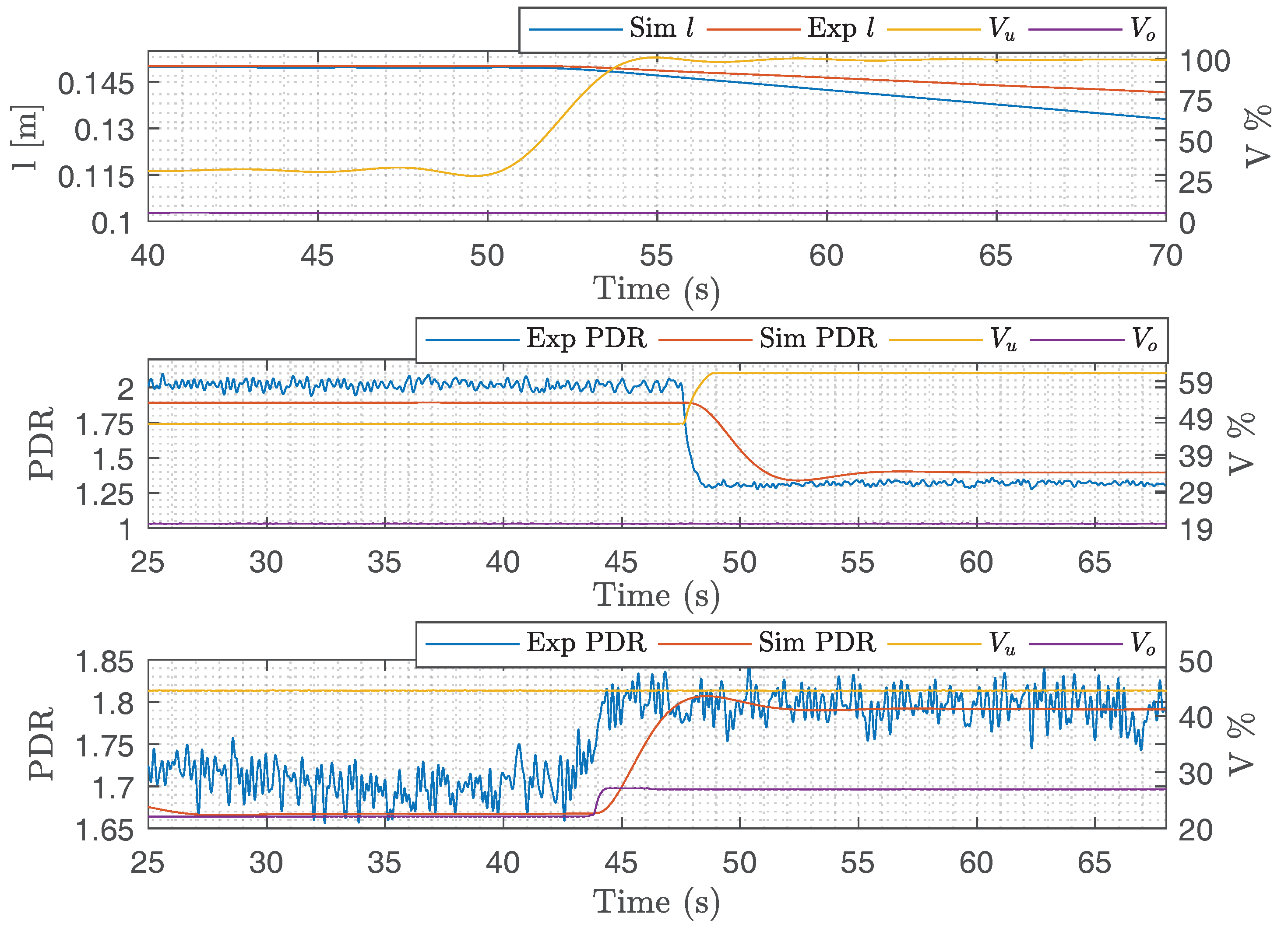
2.2. Model Validation
Figure 3 illustrates the validation of the de-oiling system’s model, divided into three plots, where the first plot represents the relationship between the underflow valve and the level, the second between the underflow valve and the PDR, and the third between the overflow valve and the PDR. The simulated l decreases linearly after the step input on as expected, although the model has a faster data dynamic than the experimental data One of the reasons for this is the natural drift in the pressure inside of the gravity separator, which slowly decreases with a full opening of the underflow valve. This part is neglected in the model development, as during nominal operation of the system the underflow valve will not be actuated to a fully open position for excessive periods and from this experiment we see that the deviation from the experimental data is small around the operating point but exceeds as we move away from the operating point. Both the hydrocyclone models that were identified have a good fitness to the real data, although the simulation has a slower dynamic than the real system, in particular the model describing the relationship between the underflow valve and the PDR. This is partially due to the linear model’s performance in wide operating ranges, as the underflow valve is set to actuate relatively more than the overflow valve with respect to its impact on the PDR. This is reflected in the large deviation in the PDR, from approximately 2 to approximately 1.4.
3. Synthesis of the Robust Control Solution
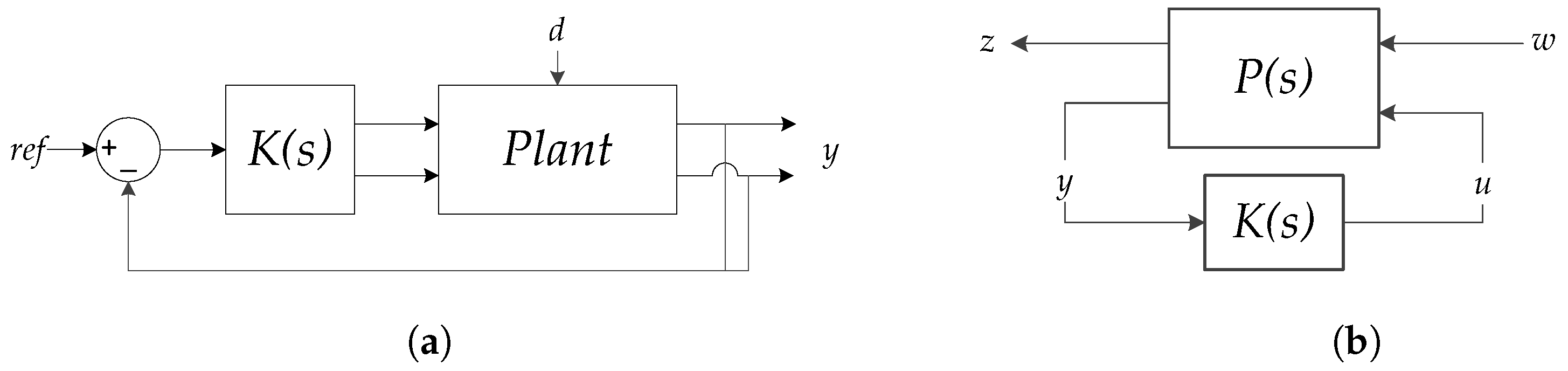
We aim at designing a controller , which governs the plant as shown in Figure 4a. Following the standard representation of the robust H control solution shown in Figure 4b, our system can be rearranged following this configuration, and the closed-loop inter-connected system is obtained based on the general definition shown in Equation (4).
The external inputs to the system defined by w, are the reference and the disturbance and the represents the linear model’s deviation from the linearized equilibrium value. The output signals are defined as z, and consist of l and PDR. The vector of control signals defined as u, consists of the input variables and . The vector of the available measurements defined as y, consists of the error signals and (). It can be denoted by:
where:
which leads to the matrix representation of our system’s interconnected system P in Equation (7).
3.1. Numerical Solvability
We intend to develop the robust control solution using methods provided in [40,41], where the interconnected system P has to satisfy several assumptions listed below:
3.1.1. Assumption 1
First, the linear system must be controllable from the control inputs u and observable from the measurement output y, which is a requirement to find a stabilizing controller K [42]. The dynamic system consisting of the pair must be controllable [43]. The rank of the controllability matrix has been calculated using the system matrices, and it leads to a full column rank, indicating that the system is controllable. The dynamic system consisting of the pair must be observable [43]. The rank of the observability matrix has been calculated using the system matrices, A and C, and this leads to a full row rank, indicating that the system is observable.
3.1.2. Assumption 2
and must be full column and row rank, which ensures that the controller is proper, in our case is full row rank, while is not. Thus, a control weighting matrix is added to ensure that is a full column rank only for design purpose.
3.1.3. Assumption 3
It must show that the matrix in Equation (8) has full column rank for all frequency range. The rank has been calculated for frequencies in the range 0–10 rad/s, with a step of 0.001 rad/s, and with respect to the considered system P the rank of matrix in Equation (8) is always full column rank, plus it is observed that this considered system doesn’t have any right half-plane transmission zero, thus this assumption is fulfilled.
3.1.4. Assumption 4
It must show that the matrix in Equation (9) has full row rank for all . The rank has been calculated for frequencies in the range 0–10 rad/s, with a step of 0.001 rad/s, and with respect to the considered system P the rank of matrix in Equation (9) is always full row rank; in addition, it is observed that this considered system does not have any right half-plane transmission zero, thus this assumption is fulfilled.
with all the above assumptions satisfied the controller K can be designed.
3.2. H Controller Synthesis
To ensure that an admissible controller exists for a given , such that , i.e., to ensure the existence of the H suboptimal controller, a test is done which ensures that the following three conditions hold:
- H with ;
- J with ; and
- .
If the conditions above are satisfied then all rational internally stabilizing controller K(s) satisfying are given by:
where:
The H controller solution is found by solving the two Riccati equations, i.e., finding the solutions to the Riccati equations and , refer to Equation (12), and the state feedback and output injection matrices F and L. For detailed definition of the Hamiltonian matrices and H, and F and L, refer to [40].
3.3. The Designed H Controller
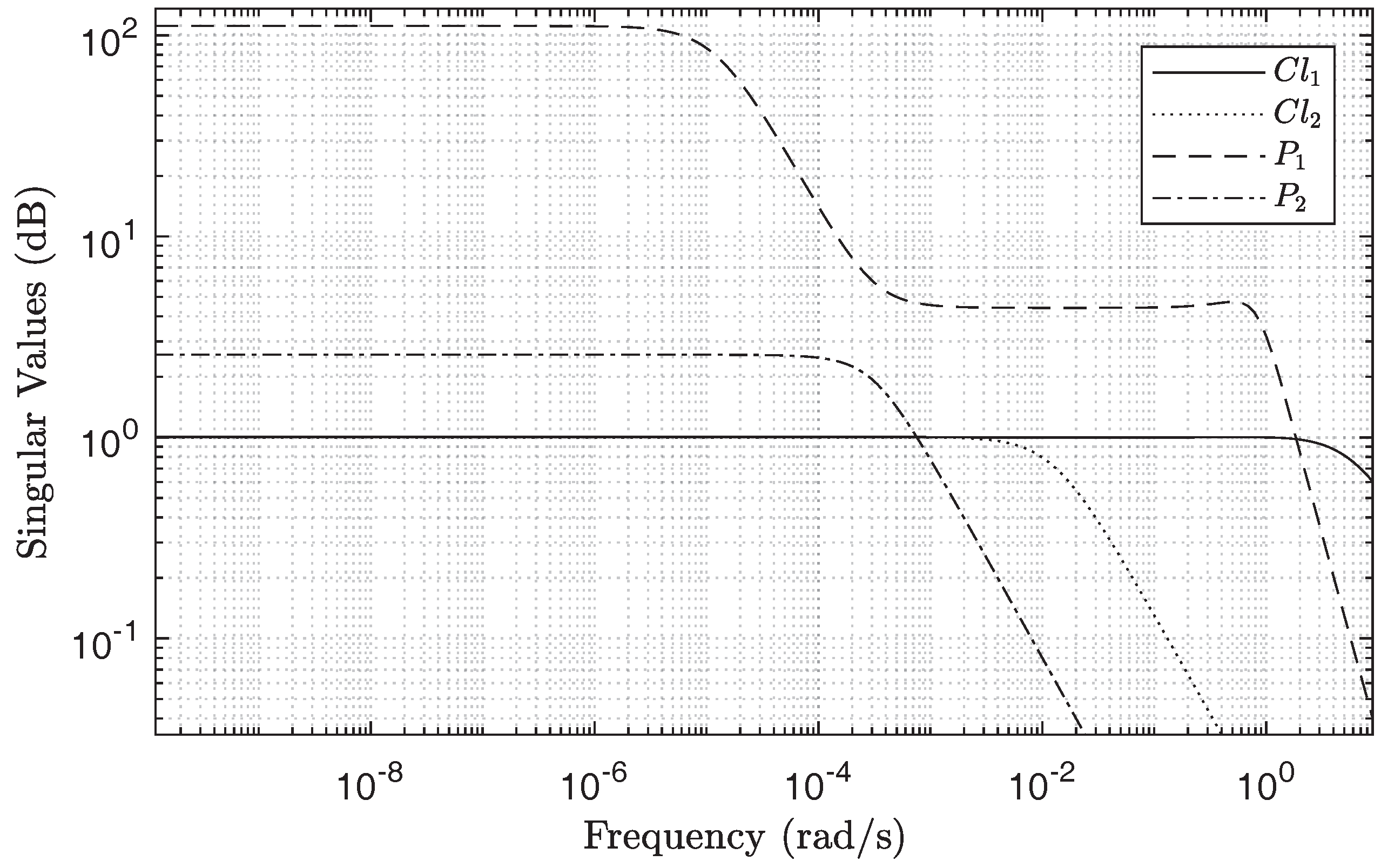
The numerically optimal upper bound value is calculated as 1.0059, and the singular values are plotted for both the open loop and closed loop systems from each of the two inputs, as shown in Figure 5. From the singular values shown in Figure 5, it can be seen that singular values are reduced for all frequencies with respect to both inputs. In addition, we see that the H controller gives a relatively flat response as it minimizes the peak of the frequency response.
4. Benchmark PID Control Solution
The PID control structure is designed to emulate the offshore scenario and thus to function as a benchmark control solution for evaluation of our newly developed H control solution. The most common control structure in the Danish sector of the North Sea is the one shown in Figure 1, where there are two individual PID controllers for the two manipulated variables, and , using the two feedback parameters, l and PDR. Following this control structure, the PID solution tested in this paper was manually tuned with an aim to emulate similar performance as was observed from the real-life scenarios (we have the real-life data from the cooperated operators collected from a specific North-sea field shown in Figure 2). In Table 2, the offshore PID controller performance during slugging regime is compared to the benchmark PID in simulations and in our experiments; the respective data are shown in Figure 2, Figure 6 and Figure 8.
From the pilot plant and offshore perspective the benchmark PID controller performs close to the offshore controller. The offshore system’s was saturated in a wide range of the data collected, which emphasizes the dominance of and the relatively small impact has on the amplitude of l and the PDR in comparison to the . In general, the behaviour of the benchmark PID controller with regard to the pilot plant implementation replicates the behaviour of the offshore PID controller well, for example the PDR oscillates heavily during fluctuating flow while the level stays relatively stable. The benchmark PID control solution is thus suitable to be used for evaluating the H, as it performs closely to the real offshore system.
5. Performance Analysis via Simulation
This section presents a comparison of the performances of the H control solution and the benchmark PID control solution in simulations. The comparisons were made for the following performance aspects: (a) reference tracking; and (b) disturbance rejection (both steady state and dynamic).
5.1. Description of the Testing Scenarios
Three test scenarios were performed, and the individual scenarios are shown in Table 3.
5.1.1. Scenario ①
This scenario aims at testing both the controllers’ step response and their steady state reference tracking performance, by stepping the reference of l.
5.1.2. Scenario ②
This scenario aims at investigating both the controllers’ step response and their steady state performance towards a step in the reference of PDR.
5.1.3. Scenario ③
This evaluates both controllers’ robustness towards additive disturbances, in this case the disturbance is set to emulate a severe slugging scenario which impacts the gravity separator’s l and thus affects both the valves due to the coupling. The aim of this test is to evaluate both controllers’ dynamic disturbance rejection and identify the controller that has an advantage in reducing the impact of fluctuating flows to the system.
5.2. Simulation Results
The results of the simulated PID and H control solutions, following the scenarios defined in Table 3, are plotted in two columns as shown in Figure 6. Each column consists of three individual plots where: the top plot shows the PDR and its reference, the second plot the valve positions in (%) and the bottom plot l and its reference in (mm). The minimum and maximum boundaries for the PDR and l are illustrated with horizontal dashed lines and each scenario is indicated by vertical dotted lines and labeled as ①, ② and ③. The simulations results were set to run for 3000 s to initialize the system and allow it to reach steady state before introducing scenario ①. The reference tracking of the PID control solution performs well both with respect to l and PDR as expected. The PID controller sacrifices valve excitation where both valves are being aggressively regulated by the individual PID control loops each tracking its individual reference. The less dominant PDR loop, suffers during the level step, where has a significant impact on the PDR as is expected and seen in the offshore data in Figure 2. The introduction of fluctuating disturbance, in scenario ③, has a direct impact on l and with respect to the PID control solution, similar to the offshore data. The impact on the PDR and is slightly different due to the saturation of in the offshore case. The reference tracking performance of the H control solution with respect to l, has a steady state offset from the reference, with an error of 35 mm, before and after the reference step in l; and a steady state offset error of 55 mm after the PDR step. The relatively large error after the step in the PDR reference occurs as the H control solution explicitly takes care of the trade-off between performances for set-point tracking and disturbance injection, while the PID controller (current one) is developed mainly for having a good set-point tracking performance. The reference tracking of the PDR with the H control solution, has a steady state offset with an negligible error in scenario ①. In scenario ②, an steady state error of 0.06 PDR occurs and it continues in scenario ③.
The performance of the H control solution is better in comparison to the PID control solution when a disturbance is added, in particular with respect to to the PDR in scenario ③, where the PDR fluctuations are insignificant. This is reflected in both and , whose actuation is reduced when compared to the PID control solution with respect to scenario ③, i.e., disturbance rejection.
6. Scaled Pilot Plant Implementation
A scaled pilot plant of an offshore de-oiling facility was designed and constructed at our laboratory in Aalborg University, Esbjerg, Denmark, for more information refer to [20,24,27,28,47,48]. The Benchmark PID control solution and the H control solution were implemented onto our pilot plant using Matlab’s Simulink Real-Time environment, which is interfaced with the pilot plant through National Instruments data acquisition cards.
6.1. Scaled Pilot Plant Experiment Description
The PID and the H controllers were implemented on the scaled pilot plant and tested under different operating conditions, similar to those tested during the simulations in Section 5. The experimental scenarios are presented in Table 4. The first three scenarios, ④, ⑤, and ⑥, are under nominal conditions and are similar to the ones made for the simulated controllers (see Table 3). An additional severe scenario ⑦ is included in this experiment. Scenario ⑦ differs from the rest with respect to the input which was designed to emulate severe offshore conditions. It is a generated sine wave with a frequency of 0.003 Hz multiplied with white Gaussian noise and the frequency spectrum of the signal is shown in Figure 7.
The goal of this experiment was to test the system’s robustness towards severe slugging emulated by manipulating the such that large fluctuations as experienced by offshore de-oiling systems were formed, refer to Figure 2.
The desired operating conditions of the two control parameters, the PDR and the l for the scaled pilot plant are presented in Table 5.
6.2. Results of Experiments Performed on the Scaled Pilot Plant
The result of scenarios ④ to ⑥ are plotted in Figure 8, and the result of scenario ⑦ is plotted in Figure 9.
6.2.1. Experiment Results for Scenario ④
The tracking performance of the PID control solution in the initialization phase is perfect, and during scenario ④ the steady state l reference is tracked perfectly. The sacrifice during scenario ④ is that the PID control solution fully chokes , which results in a rapid increase of the PDR reaching a peak value of 415. PDR reaches its reference after approximately 70 s.
Reference tracking of l is not managed by the H control solution, with a maximum steady state deviation of 28 mm before, and mm after ④ respectively. The PDR remains relatively steady, with a steady state error of approximately 0.12 PDR.
6.2.2. Experiment Results for Scenario ⑤
The reference tracking of the PDR during scenario ⑤ is perfectly managed by the PID control solution, where approximately 4% adjustment of (% to %) manages the reference step with relatively no delay and fast PDR dynamics. The effect on the l feedback loop is negligible.
The H control solution’s reference tracking of the PDR during the PDR step happens instantaneously, mostly to be attributed to the cooperative action of the two valves. Although the H control solution has a steady state error of approximately 0.1 PDR, the H control solution has less oscillations than the PID control solution, peak-to-peak amplitude of the two signals is 0.07 PDR and 0.23 PDR for the H and the PID control solution respectively. During scenario ⑤, the level drifts slowly by approximately 8.5 mm in the case of the H control solution and thus remains well within its safety boundary.
6.2.3. Experiment Results for Scenario ⑥
During scenario ⑥, l has minor oscillations with a steady state error of 1.4%, under the PID control solution. The consequence of this good reference tracking are oscillations of with a peak-to-peak amplitude of %. Which are directly translated into an oscillating PDR value which at times reaches PDR (steady state error of 2.1 PDR), with a peak-to-peak amplitude of PDR. The PDR feedback loop compensates by adjusting , which results in oscillations in with a peak-to-peak amplitude of %.
During scenario ⑥, the performance of the H control solution is barely affected by the oscillations in . The PDR continues unchanged from scenario ⑤ with a steady state error of 0.11 PDR (4.6%) and relatively low peak-to-peak amplitude of . Besides PDR, l is equivalently little affected by the disturbance, at it reaches a steady state error of 41 mm, which is still far from the boundary.
6.2.4. Experiment Results for Scenario ⑦
During scenario ⑦ (Figure 9), the PID control solution performs well with respect to tracking the l reference with a maximum steady state error of approximately 5.6 mm (approximately 3.7%), which is translated in an aggressive actuation of , between 0% and 60%. This has a direct impact on and the PDR, where experiences severe saturation in the fully open position, which accounts for 45% of the experiments duration with the longest period being 174 s. This has a severe impact on the PDR which oscillates with values as low as 1, during %, and as high as 21 PDR (outside the y-axis range, at 2087 s).
The actuation of is reduced with the H control solution, with a maximal peak-to-peak actuation of approximately 6%, which results in reduced reference tracking of l, which reaches a steady state error of approximately 130 mm (approximately 86%). In comparison, reference tracking of the PDR performs better with a maximal steady state error of 0.23 PDR (11.5%), and a relatively low oscillation, which is most likely an effect of measurement noise; is not severely actuated having a peak-to-peak amplitude of 34%, (staying within the range 25–59%).
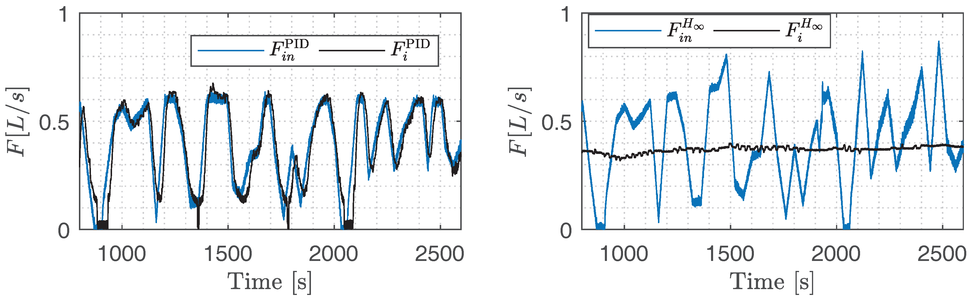
6.3. Transmission of Fluctuations in
In Figure 10, it can be observed that is conveyed directly to , which potentially could reduce the hydrocyclone’s performance as was shown in [20]. Reducing the transmission of these oscillations from to is therefore crucial. This has been successfully achieved using the H control solution, where the transmission has been filtered significantly.
7. Discussion
7.1. Simulation Results
A benchmark PID control solution was designed and tuned to emulate the performance of the offshore system, and in the simulations and experiments made on the scaled pilot plant it was possible to emulate the offshore performance. As seen throughout the simulation results, the H control solution has a reduced reference tracking which kept the controllable parameters and from saturating. The benchmark PID control solution saturated in favor of the PDR reference tracking in scenario ⑦. With the H control solution, the MIMO control structure leads to cooperation of both the controllable parameters. The result is a more relaxed valve actuation, which benefits the PDR, unlike the PID control solution where each valve is actuated independently and more aggressively as the two sub-systems work against each other resulting in a more oscillating PDR, same was observed in the offshore data in Figure 2. With respect to the scenario ⑥, the H control solution’s reference tracking is sacrificed which results in the controlled variables being within safe ranges. In comparison, the PID control solution saturates the . The sacrifice which the H control solution makes is a fluctuating l, which if kept within certain bounds, is inconsequential for this type of system as discussed in Section 1. The relaxed PDR response leads to a reduced actuation of the valves, especially of and thus results in a smoother and thereby an overall increased de-oiling efficiency. The saturation of valves, as in the case of the PID control solution, renders the system uncontrollable and l can as a result exceed its minimum or maximum level which would lead to eventual system instability.
7.2. Experimental Results
The reference tracking by the PID control solution and the lack of cooperation between the two sub-controllers affects the performance of the system. The reference tracking of l often results in saturation of which is of great consequence for the PDR, as the is less dominant and PID control solution cannot compensate for this effect due to the saturated . The result of this behaviour is specifically expressed during the oscillating , in the ⑥ scenario in Figure 8. During ⑥, the peak-to-peak amplitude of PDR with respect to the PID control solution was , reaching values as high as 21, which is comparable to the real offshore scenario shown in Figure 2, Section 1. This is far outside the operating range (see Table 5), and such performance will result in large concentrations of water in the overflow, which then necessitates recirculation through the separation process. Under the same conditions, the PDR with respect to the H control solution had a peak-to-peak amplitude , which is a considerable 22 times lower oscillating amplitude.
8. Conclusions
Slugging flow, which causes the gravity separator inlet flow rate into the offshore de-oiling facilities to fluctuate severely, is an unmeasurable disturbance and has negative effects on the de-oiling process. The controllable parameters in the de-oiling system are the level of the gravity separator l and the pressure drop ratio (PDR) of the hydrocyclone, which are controlled by the actuation of the underflow valve () and overflow valve () respectively. An initial investigation showed that the current PID control paradigm and the inherent coupling of the unit processes of the de-oiling facilities, the gravity separator and the hydrocyclone, results in a system which has poor disturbance rejection. Thus, fluctuating is observed to propagate to the downstream hydrocyclone, which in previous studies was shown to have a direct impact on the hydrocyclone’s de-oiling efficiency . It was therefore concluded that the de-oiling system would perform better if its disturbance rejection was improved. In this study, we have investigated the benefit of a robust H control solution in comparison to a benchmark PID control solution that is used for offshore de-oiling. A MIMO model of the de-oiling process was developed, based on which a robust suboptimal H control solution was designed. The H control solution was tested in simulations and then implemented and tested on the scaled pilot plant. In the simulations, where the H control solution was compared to a benchmark PID control solution, the H control solution facilitated disturbance attenuation and provided a more relaxed actuation of and . The conventional PID control solution, however, saturated the while trying to track the level reference, a scenario similar to what was observed in data from offshore facilities during slugging flow.
The results from the experiments performed on the scaled pilot plant further proved that the H control solution was better at handling the disturbance , and in all the circumstances that were tested, it kept the system stable. The benchmark PID control solution once again under certain circumstances saturated the controllable parameters. The reduced reference tracking of l by the H control solution, resulted in almost perfect damping of the transmission of the disturbance into . In addition, in real life scenarios, the reduced valve actuation by the H control solution could reduce the wear and tear on the system.
In future work, the model of the de-oiling system will be extended to include the de-oiling hydrocyclone efficiency in the model and control design.
Acknowledgments
The authors would like to thank the support from the Danish Innovation Foundation (via PDPWAC Project (J.nr. 95-2012-3)). Thanks also go to colleagues J. P. Stigkær, A. Aillos, K. G. Nielsen and T. I. Bruun from Mærsk Oil A/S; and colleagues P. Sørensen, A. Andreasen and Jakob Biltoft from Rambøll Oil & Gas A/S for many valuable discussions and supports. Thanks also go to AAU colleagues C. Mai, K. Jepsen, L. Hansen, M. Bram and D. Hansen for their contributions to this project.
Author Contributions
Petar Durdevic and Zhenyu Yang conceived and designed the experiments; Petar Durdevic performed the experiments; Petar Durdevic and Zhenyu Yang analyzed the data; and Petar Durdevic wrote the paper.
Conflicts of Interest
The founding sponsors had no role in the design of the study; in the collection, analyses, or interpretation of data; in the writing of the manuscript, and in the decision to publish the results.
References
- Bamberg, J. British Petroleum and Global Oil 1950–1975: The Challenge of Nationalism; British Petroleum Series; Cambridge University Press: Cambridge, UK, 2000. [Google Scholar]
- Ekins, P.; Vanner, R.; Firebrace, J. Zero emissions of oil in water from offshore oil and gas installations: Economic and environmental implications. J. Clean. Prod. 2007, 15, 1302–1315. [Google Scholar] [CrossRef]
- Stephenson, M. A survey of produced water studies. In Produced Water; Springer: Berlin/Heidelberg, Germany, 1992; pp. 1–11. [Google Scholar]
- Bailey, B.; Crabtree, M.; Tyrie, J.; Elphick, J.; Kuchuk, F.; Romano, C.; Roodhart, L. Water control. Oilfield Rev. 2000, 12, 30–51. [Google Scholar]
- Veil, J.A.; Puder, M.G.; Elcock, D.; Redweik, R.J., Jr. A White Paper Describing Produced Water From Production of Crude Oil, Natural Gas, and Coal Bed Methane; Technical Report; Argonne National Laboratory: Lemont, IL, USA, 2004; Volume 63.
- Danish Production of Oil, Gas and Water (Danish Energy Agency). Available online: https://ens.dk/en/our-services/oil-and-gas-related-data/monthly-and-yearly-production (accessed on 1 November 2016).
- Miljoestyrelsen. Status for Den Danske Offshorehandlingsplan Til Udgangen Af 2009. Miljoestyrelsen. Available online: http://www.ft.dk/samling/20101/almdel/MPU/bilag/66/903508.pdf (accessed on 1 October 2017).
- Miljoestyrelsen. Afsluttende rapport for de danske offshorehandlingsplaner 2005–2010. Miljoestyrelsen. Available online: http://mst.dk/media/91455/Bilag%203%20Statusrapport%20OHP%202013%20rev%20(2).pdf (accessed on 1 October 2017).
- Methodology for the Sampling and Analysis of Produced Water and Other Hydrocarbon Discharges. Available online: https://www.gov.uk/guidance/oil-and-gas-offshore-environmental-legislation (accessed on 3 November 2016).
- OSPAR Commission, About OSPAR. Available online: https://www.ospar.org/about (accessed on 10 January 2018).
- Miljoestyrelsen. Generel Tilladelse for MæRsk Olie Og Gas A/S (MæRsk Olie) Til Anvendelse, Udledning Og Anden Bortskaffelse Af Stoffer Og Materialer, Herunder Olie Og Kemikalier I Produktions-Og Injektionsvand Fra Produktionsenhederne Halfdan, Dan, Tyra Og Gorm for Perioden 1. Januar 2017-31. December 2018. Miljoestyrelsen. Available online: http://mst.dk/media/92144/20161221-ann-generel-udledningstilladelse-for-maersk-olie-og-gas-2017-18.pdf (accessed on 19 October 2017).
- Monnery, W.D.; Svrcek, W.Y. Successfully Specify 3-Phase Separators. Chem. Eng. Prog. 1994, 90, 29–40. [Google Scholar]
- Sayda, A.F.; Taylor, J.H. Modeling and control of three-phase gravilty separators in oil production facilities. In Proceedings of the American Control Conference, New York, NY, USA, 9–13 July 2007; pp. 4847–4853. [Google Scholar]
- Thew, M. Hydrocyclone redesign for liquid-liquid separation. Chem. Eng. (London) 1986, 427, 17–23. [Google Scholar]
- Husveg, T.; Rambeau, O.; Drengstig, T.; Bilstad, T. Performance of a deoiling hydrocyclone during variable flow rates. Miner. Eng. 2007, 20, 368–379. [Google Scholar] [CrossRef]
- Ditria, J.; Hoyack, M. The separation of solids and liquids with hydrocyclone-based technology for water treatment and crude processing. In SPE Asia Pacific Oil and Gas Conference; Society of Petroleum Engineers: London, UK, 1994. [Google Scholar]
- VORTOIL Deoiling Hydrocyclones. Available online: http://www.slb.com/~/media/Files/processing-separation/product-sheets/vortoil-ps.pdf (accessed on 20 October 2017).
- Husveg, T.; Johansen, O.; Bilstad, T. Operational Control of Hydrocyclones during Variable Produced Water Flow Rates—Frøy Case Study. SPE Prod. Oper. 2007, 22, 294–300. [Google Scholar] [CrossRef]
- Husveg, T. Operational Control of Deoiling Hydrocyclones and Cyclones for Petroleum Flow Control. Ph.D. Thesis, University of Stavanger, Stavanger, Norway, 2007. [Google Scholar]
- Durdevic, P.; Raju, C.S.; Bram, M.V.; Hansen, D.S.; Yang, Z. Dynamic Oil-in-Water Concentration Acquisition on a Pilot-Scaled Offshore Water-Oil Separation Facility. Sensors 2017, 17, 124. [Google Scholar] [CrossRef] [PubMed]
- Di Meglio, F.; Kaasa, G.O.; Petit, N.; Alstad, V. Model-based control of slugging: Advances and challenges. IFAC Proc. Vol. (IFAC PapersOnline) 2012, 1, 109–115. [Google Scholar] [CrossRef]
- Sausen, A.; de Campos, M.; Sausen, P. The Slug Flow Problem in Oil Industry and Pi Level Control; InTech Open Access Publisher: London, UK, 2012. [Google Scholar]
- Pedersen, S.; Durdevic, P.; Yang, Z. Review of Slug Detection, Modeling and Control Techniques for Offshore Oil & Gas Production Processes. IFAC PapersOnLine 2015, 48, 89–96. [Google Scholar]
- Durdevic, P.; Pedersen, S.; Yang, Z. Challenges in Modelling and Control of Offshore De-oiling Hydrocyclone Systems. J. Phys. Conf. Ser. 2017, 783, 012048. [Google Scholar] [CrossRef]
- Meldrum, N. Hydrocyclones: A Solution to Produced-Water Treatment. In SPE Production Engineering; University of Michigan: Ann Arbor, MI, USA, 1988; Volume 3, pp. 669–676. [Google Scholar]
- Thew, M.; Smyth, I. Development and performance of oil-water hydrocyclone separators: A review. In Proceedings of the IMM Conference on Innovation in Physical Separation Technologies, Southampton, UK, 1 January 1998. [Google Scholar]
- Durdevic, P.; Pedersen, S.; Yang, Z. Operational Performance of Offshore De-oiling Hydrocyclone Systems. In Proceedings of the 43rd Annual Conference of the IEEE Industrial Electronics Society (IECON), Beijing, China, 29 October–1 November 2017; Volume 43, pp. 6905–6910. [Google Scholar]
- Durdevic, P. Real-Time Monitoring and Robust Control of Offshore De-oiling Processes. Ph.D. Thesis, Aalborg University, Aalborg, Denmark, 2017. [Google Scholar]
- Mokhatab, S.; Poe, W.; Speight, J. Handbook of Natural Gas Transmission and Processing; Chemical, Petrochemical & Process, Gulf Professional Pub.: London, UK, 2006. [Google Scholar]
- Judd, S.; Qiblawey, H.; Al-Marri, M.; Clarkin, C.; Watson, S.; Ahmed, A.; Bach, S. The size and performance of offshore produced water oil-removal technologies for reinjection. Sep. Purif. Technol. 2014, 134, 241–246. [Google Scholar] [CrossRef]
- Yang, Z.; Juhl, M.; Lø hndorf, B. On the innovation of level control of an offshore three-phase separator. In Proceedings of the IEEE International Conference on Mechatronics and Automation, ICMA 2010, Xi’an, China, 4–7 August 2010; pp. 1348–1353. [Google Scholar]
- Rietema, K.; Maatschappij, S.I.R. Performance and design of hydrocyclones—III: Separating power of the hydrocyclone. Chem. Eng. Sci. 1961, 15, 310–319. [Google Scholar] [CrossRef]
- Wolbert, D.; Ma, B.-F.; Aurelle, Y.; Seureau, J. Efficiency estimation of liquid-liquid Hydrocyclones using trajectory analysis. AIChE J. 1995, 41, 1395–1402. [Google Scholar] [CrossRef]
- Thew, M.T. Cyclones for oil/water separation. In Encyclopaedia of Separation Science, 4th ed.; Academic Press: Cambridge, MA, USA, 2000; pp. 1480–1490. [Google Scholar]
- Kharoua, N.; Khezzar, L.; Nemouchi, Z. Hydrocyclones for de-oiling applications—A review. Pet. Sci. Technol. 2010, 28, 738–755. [Google Scholar] [CrossRef]
- Thew, M.; Silk, S.; Colman, D. Determination and use of residence time distributions for two hydrocyclones. In Proceedings of the International conference on Hydrocyclones, Cambridge, UK, 1–3 October 1980; pp. 225–248. [Google Scholar]
- Young, G.; Wakley, W.; Taggart, D.; Andrews, S.; Worrell, J. Oil-water separation using hydrocyclones: An experimental search for optimum dimensions. J. Petrol. Sci. Eng. 1994, 11, 37–50. [Google Scholar] [CrossRef]
- Bram, M.V.; Hassan, A.A.; Hansen, D.S.; Durdevic, P.; Pedersen, S.; Yang, Z. Experimental modeling of a deoiling hydrocyclone system. In Proceedings of the 20th International Conference on Methods and Models in Automation and Robotics, Miedzyzdroje, Poland, 24–27 August 2015; pp. 1080–1085. [Google Scholar]
- Durdevic, P.; Pedersen, S.; Bram, M.; Hansen, D.; Hassan, A.; Yang, Z. Control Oriented Modeling of a De-oiling Hydrocyclone. IFAC PapersOnLine 2015, 48, 291–296. [Google Scholar] [CrossRef]
- Zhou, K.; Doyle, J.C.; Glover, K. Robust and Optimal Control; Prentice Hall: Upper Saddle River, NJ, USA, 1996; Volume 40. [Google Scholar]
- Zhou, K.; Doyle, J.C. Essentials of Robust Control; Prentice Hall: Upper Saddle River, NJ, USA, 1998; Volume 104. [Google Scholar]
- Glover, K.; Doyle, J.C. State-space formulae for all stabilizing controllers that satisfy an H∞-norm bound and relations to relations to risk sensitivity. Syst. Control Lett. 1988, 11, 167–172. [Google Scholar] [CrossRef]
- Kalman, R.E. Mathematical description of linear dynamical systems. J. Soc. Ind. Appl. Math. Ser. A Control 1963, 1, 152–192. [Google Scholar] [CrossRef]
- Gu, D.; Petkov, P.; Konstantinov, M.M. Robust Control Design With MATLAB, 2nd ed.; Springer Science & Business Media: New York, NY, USA, 2005. [Google Scholar]
- Skogestad, S.; Postlethwaite, I. Multivariable Feedback Control: Analysis and Design; Wiley: New York, NY, USA, 2007; Volume 2. [Google Scholar]
- Balas, G.; Chiang, R.; Packard, A.; Safonov, M. Robust control toolbox. In For Use with Matlab. User’s Guide, Version 3; The Mathworks, Inc.: Natick, MA, USA, 2005; Volume 3. [Google Scholar]
- Yang, Z.; Pedersen, S.; Durdevic, P. Cleaning the produced water in offshore oil production by using plant-wide optimal control strategy. In Proceedings of the 2014 Oceans—St. John’s, St. John’s, NL, Canada, 14–19 September 2014; pp. 1–10. [Google Scholar]
- Yang, Z.; Pedersen, S.; Durdevic, P.L.; Mai, C.; Hansen, L.; Jepsen, K.L.; Aillos, A.; Andreasen, A. Plant-wide Control Strategy for Improving Produced Water Treatment. In Proceedings of the 2016 International Field Exploration and Development Conference (IFEDC), Beijing, China, 11–12 August 2016. [Google Scholar]
Figure 1.
Schematic Piping and Instrumentation Diagram (P&ID) of an offshore de-oiling facility, including the control loops.
Figure 1.
Schematic Piping and Instrumentation Diagram (P&ID) of an offshore de-oiling facility, including the control loops.
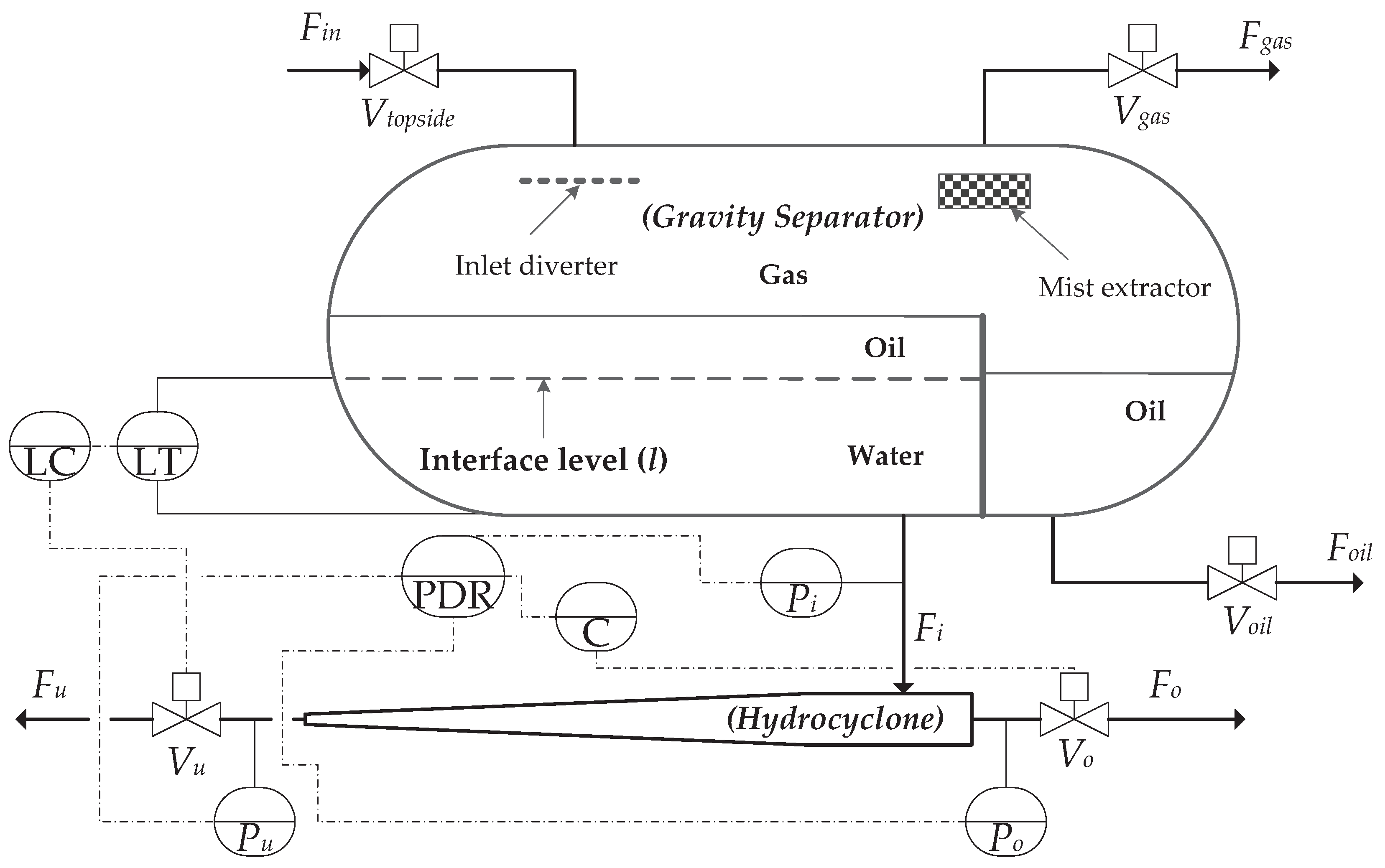
Figure 2.
Data collected from an offshore produced water treatment facility in the Danish sector of the North Sea; the set-points are (l mm & PDR ).
Figure 2.
Data collected from an offshore produced water treatment facility in the Danish sector of the North Sea; the set-points are (l mm & PDR ).

Figure 3.
Step response validation of the model, with respect to the gravity separator and the hydrocyclone.
Figure 3.
Step response validation of the model, with respect to the gravity separator and the hydrocyclone.

Figure 4.
(a) The closed loop system; and (b) the standard representation of the Robust H control solution.
Figure 4.
(a) The closed loop system; and (b) the standard representation of the Robust H control solution.

Figure 5.
Singular values of P, where the open-loop system , and the closed-loop system , where , for frequencies between 0 and the Nyquist frequency /.
Figure 5.
Singular values of P, where the open-loop system , and the closed-loop system , where , for frequencies between 0 and the Nyquist frequency /.

Figure 6.
Performance analysis of the H control solution in comparison to the PID control solution in simulations. The scenario changes are indicated by dotted lines, while the minimum and maximum limits are represented with dashed horizontal lines.
Figure 6.
Performance analysis of the H control solution in comparison to the PID control solution in simulations. The scenario changes are indicated by dotted lines, while the minimum and maximum limits are represented with dashed horizontal lines.

Figure 7.
Frequency spectrum of the input signal .
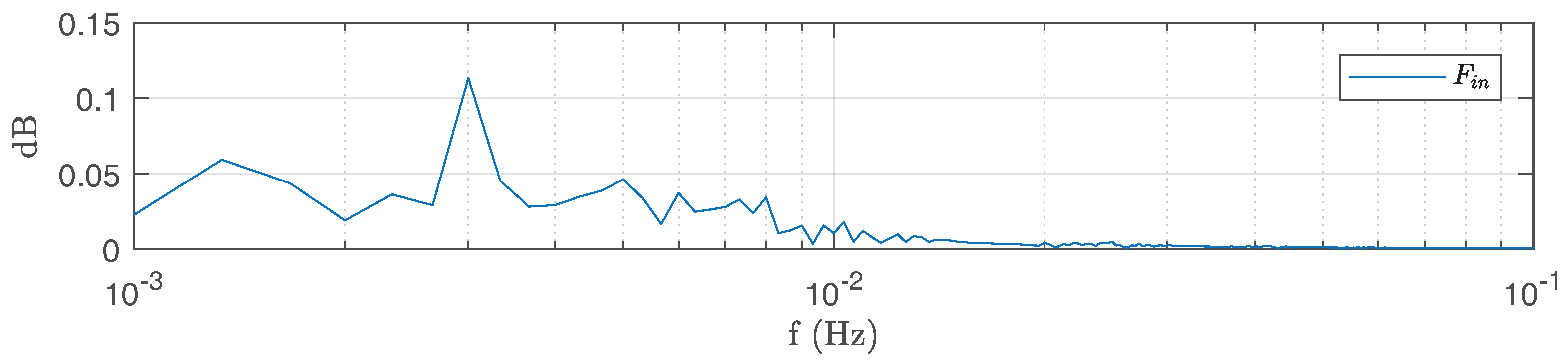
Figure 8.
Performance analysis of the H control solution in comparison to the PID control solution in the pilot plant experiments under Nominal operation; the scenario changes are indicated by dotted lines, while the minimum and maximum limits are represented with dashed horizontal lines.
Figure 8.
Performance analysis of the H control solution in comparison to the PID control solution in the pilot plant experiments under Nominal operation; the scenario changes are indicated by dotted lines, while the minimum and maximum limits are represented with dashed horizontal lines.

Figure 9.
Test results for severe operation ⑦, where is fluctuating in the range 0–0.8 L/s.
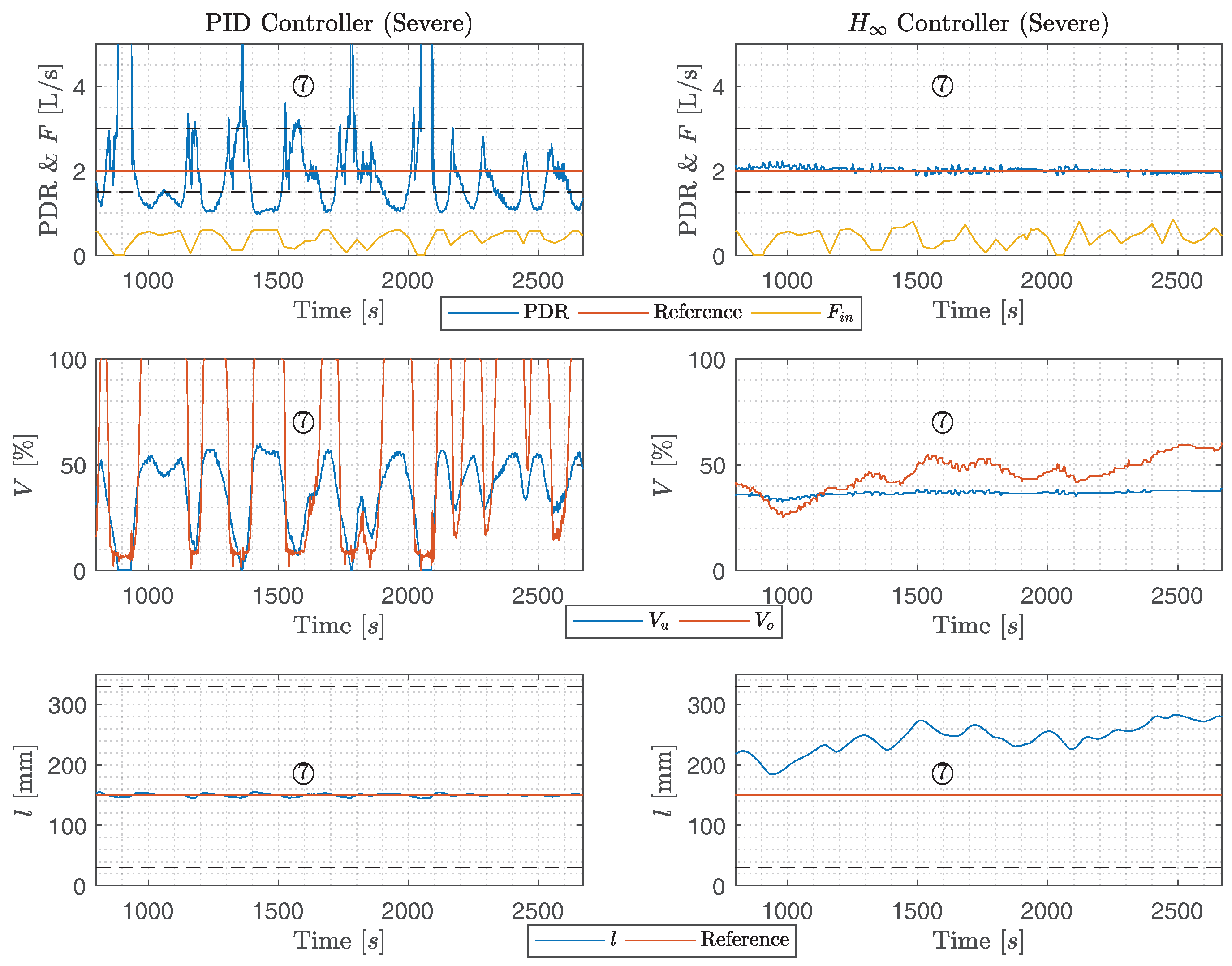
Figure 10.
Comparison of flow propagation through the de-oiling system, from to , with respect to the PID control solution (top plot) and the H control solution. Analysis is based on the experimental data from Figure 9, i.e., scenario ⑦.
Figure 10.
Comparison of flow propagation through the de-oiling system, from to , with respect to the PID control solution (top plot) and the H control solution. Analysis is based on the experimental data from Figure 9, i.e., scenario ⑦.

Table 1.
System parameters of the state space formulation relevant to Equation (3).
Table 1.
System parameters of the state space formulation relevant to Equation (3).
| A | B | C |
|---|---|---|
Table 2.
Benchmark PID control solution’s evaluation data. Maximal peak-to-peak oscillating amplitude of the valves and the maximum percentile error of l and the PDR.
Table 2.
Benchmark PID control solution’s evaluation data. Maximal peak-to-peak oscillating amplitude of the valves and the maximum percentile error of l and the PDR.
| Platform | l | PDR | ||
|---|---|---|---|---|
| Offshore | ||||
| Pilot Plant | ||||
| Simulation |
Table 3.
Description of the simulation scenarios.
| Scenario Name | Value & Time | Description |
|---|---|---|
| ① | l = [150 mm–170 mm] @ t = 3000 s | Step in l reference |
| ② | PDR = [2–4] @ t = 4000 s | Step in PDR reference |
| ③ | = 0.104 rad/s @ t = 5000 s | Sinusoidal disturbance input |
Table 4.
Experimental scenarios, the occurrence of the scenarios are marked with dotted vertical lines in the simulation plots.
Table 4.
Experimental scenarios, the occurrence of the scenarios are marked with dotted vertical lines in the simulation plots.
| Scenario Name | Value&Time | Description | Figure |
|---|---|---|---|
| ④ | l = [130 mm–150 mm] @ t = 1500 s | Step in l reference | Figure 8 |
| ⑤ | PDR = [2–2.4] @ t = 1800 s | Step in PDR reference | Figure 8 |
| ⑥ | = 0.104 rad/s = 0.6 L/s @ t = 2000 s | Sinusoidal input | Figure 8 |
| ⑦ | PDR = 2 | Severe scenario | Figure 9 |
Table 5.
System operating conditions.
| Parameter | Value | Unit | Alarm |
|---|---|---|---|
| PDR | 1.5–3 | PDR | No |
| l | 30–330 | [mm] | Yes |
| P | 7 | [bar] | No |
| P | 10.5 | [bar] | Yes |
| 10.5 | [bar] | Yes | |
| 1.5 | [L/s] | No |
© 2018 by the authors. Licensee MDPI, Basel, Switzerland. This article is an open access article distributed under the terms and conditions of the Creative Commons Attribution (CC BY) license (http://creativecommons.org/licenses/by/4.0/).
Share and Cite
MDPI and ACS Style
Durdevic, P.; Yang, Z. Application of H∞ Robust Control on a Scaled Offshore Oil and Gas De-Oiling Facility. Energies 2018, 11, 287. https://doi.org/10.3390/en11020287
AMA Style
Durdevic P, Yang Z. Application of H∞ Robust Control on a Scaled Offshore Oil and Gas De-Oiling Facility. Energies. 2018; 11(2):287. https://doi.org/10.3390/en11020287
Chicago/Turabian StyleDurdevic, Petar, and Zhenyu Yang. 2018. "Application of H∞ Robust Control on a Scaled Offshore Oil and Gas De-Oiling Facility" Energies 11, no. 2: 287. https://doi.org/10.3390/en11020287
Note that from the first issue of 2016, this journal uses article numbers instead of page numbers. See further details here.