Data Analytics Techniques for Performance Prediction of Steamflooding in Naturally Fractured Carbonate Reservoirs

Abstract

Thermal oil recovery techniques, including steam processes, account for more than 80% of the current global heavy oil, extra heavy oil, and bitumen production. Evaluation of Naturally Fractured Carbonate Reservoirs (NFCRs) for thermal heavy oil recovery using field pilot tests and exhaustive numerical and analytical modeling is expensive, complex, and personnel-intensive. Robust statistical models have not yet been proposed to predict cumulative steam to oil ratio (CSOR) and recovery factor (RF) during steamflooding in NFCRs as strong process performance indicators. In this paper, new statistical based techniques were developed using multivariable regression analysis for quick estimation of CSOR and RF in NFCRs subjected to steamflooding. The proposed data based models include vital parameters such as in situ fluid and reservoir properties. The data used are taken from experimental studies and rare field trials of vertical well steamflooding pilots in heavy oil NFCRs reported in the literature. The models show an average error of <6% for the worst cases and contain fewer empirical constants compared with existing correlations developed originally for oil sands. The interactions between the parameters were considered indicating that the initial oil saturation and oil viscosity are the most important predictive factors. The proposed models were successfully predicted CSOR and RF for two heavy oil NFCRs. Results of this study can be used for feasibility assessment of steamflooding in NFCRs.

1. Introduction

Consumption of liquid fuels, from both conventional and unconventional resources, will continue to be the primary source of energy in the decades to come. According to the International Energy Agency (IEA) in their World Energy Outlook 2015 report and some other reports from the U.S. Energy Information Administration (EIA) [1,2,3], global demand for oil is expected to grow from 85.7 × 10⁶ (barrel/day) [13.6 × 10⁶ m³] in 2008 to 103 × 10⁶ b/d [16.37 × 10⁶ m³] in 2030. The current global daily production rate is now 96.5 × 10⁶ b/d. This is mostly due to expected world population growth combined with increasing per capita demand in growing economies such as China and India. As the dominant trend, much of the demand for liquid fuels comes from the transportation sector, which is expected to grow at about 1.4% each year until 2035. To meet the demand for liquid fuels in 2030, additional production of 6.5 × 10⁶ b/d [1 × 10⁶ m³] will be needed. This is just a modest forecast as a reference scenario from the IEA and depending to the world economic conditions and other factors affecting the oil price and fuel consumption rate this figure is subject to change. The actual demand for oil could clearly be higher [1,2,3].

On the other hand, the sedimentary basins, especially the giant mostly carbonate fields in the Middle East, are drying fast and running out of cheap conventional oil with relatively easy production technology and in large volumes with the decline rates being on the range of 6–8% per year [4]. Obviously, there will be a growing gap between production and consumption. In the past decade, part of the gap was filled with contributions from unconventional resources. In this scenario, fossil petroleum liquids extracted from unconventional sources such as heavy oil, extra heavy oil, and bitumen will play a larger role in the decades ahead, as well. Development of non-conventional energy resources such as shale gas, shale oil and viscous oil (VO—including heavy oil, extra heavy oil, and bitumen) will fill part of the growing gap arising from a future decline in conventional oil production and the steady growth in demand for oil. However, due to large capital requirements and their relatively slow nature of development combined with technological, human capital, and economic challenges, a major and fast boost in their contribution to the global daily oil production is highly unlikely. Based on some EIA and IEA report, VO will comprise around 17% of the world daily oil production by 2035 and this also includes VO from NFCRs [1,2,3]. The current share of the VO to daily global oil production is about 8–10 × 10⁶ b/d [1.27–1.59 × 10⁶ m³/d]; roughly 10% of the total oil production, and this represents a doubling of VO production in about 25 years.

The temperature sensitivity of VO viscosity controls the flow rate in all thermal production processes. This makes the in situ oil viscosity a far more important parameter sin technical and economic assessment than API gravity. Definitions of heavy oils in the literature are inconsistent, but many including the authors recommend that heavy oils be specified as oils with viscosities >100 cP and <10,000 cP under reservoir conditions. “Bitumen” can be defined as oils having viscosity >10,000 cP in situ [5]. In this paper, VO refers to all crude oils with μ > 100 cP in situ; Heavy Oil (HO) refers to crude oil with 100 < μ < 10,000 cP in situ; Extra Heavy Oil (XHO) refers to crude oil with μ < 10,000 cP in situ but with ρ > 1.0 g/cm³; and bitumen refers to crude oil with μ > 10,000 cP in situ. A list of the various definitions and terms can be found in Dusseault and Shafiei [5] and Shafiei [6].

Almost 100% of the VO production from NFCRs comes from cold production operations in Oman, Iran, Iraq, Kuwait, Saudi Arabia, Turkey, and Mexico [6,7,8]. The VO in most of these reservoirs is mobile under reservoir conditions. Productive VO NFCRs are characterized by low matrix permeability and high fracture permeability, giving high early production that declines rapidly, leading to RFs below 3–5% in most cases [7]. Large-scale, early oil flux takes place through the high permeability and low volume fracture system, whereas the matrix-fracture interaction mainly controls the recovery efficiency and maintenance of longer-term smaller-scale production levels. VO production from NFCRs is in its very early days and is presenting major technical and economic challenges to the oil industry. These reservoirs are not yet widely commercialized and progress remains necessary for them to contribute a notable part of the daily worldwide oil production in the decades to come.

Several researchers have investigated important aspects of steamflooding (e.g., production mechanisms, productivity, wettability effects, process properties, feasibility) in homogeneous and heterogeneous porous media through experimental works, analytical modeling, and numerical modeling/simulations [9,10,11,12,13,14,15,16,17,18,19,20,21,22,23,24,25,26,27]. Most articles focus on steamflooding in unfractured (single porosity) systems. The interactive flux between the matrix block and fractures, and the consequent impact on the performance of steamflooding, are not well addressed in the literature.

Recovery Factor (RF) and Cumulative Steam to Oil Ratio (CSOR) are two critical economic parameters when evaluating an asset or designing a steamflood. Accurate determination of these key parameters is of paramount interest in predicting viability of the thermal operation. Empirical models or correlations have not been yet developed to estimate CSOR and RF for steamflooding in VO NFCRs. However, various models and correlations are reported for performance prediction and analysis of various steam injection processes for VO production from oil sands and other unconsolidated sandstone VO reservoirs [9,10,11,12,13,14,15,16,17,18,19,20,21,22,23,24,25,26,27]. Some smart models have also been developed and introduced to assess the performance of steamflooding in NFCRs [10]. Without modifications to account for the different production characteristics, such correlations or models cannot be used for VO NFCRs. Overall, it is wise to expect higher CSOR, lower RF, lower thermal efficiency, and lower ultimate profitability for VO NFCRs steam processes compared with typical oil sands or unconsolidated sandstone VO steam injection processes.

Herein, data based techniques in terms of multivariate regression are developed for rapid estimation of CSOR and RF in VO NFCRs during steamflooding based on experimental and real field data [28,29,30,31,32,33,34,35,36,37,38,39,40,41,42,43,44,45,46,47,48,49,50,51,52]. The relationships involve major parameters such as in situ fluid and reservoir properties, and process conditions (e.g., steam flow rate and quality). Previous modeling and experimental studies with the aid of a statistical methods were used to determine the key variables that most strongly affect the CSOR and RF in both homogeneous (i.e., no natural fractures such as oil sands) and fractured reservoirs experiencing steamflooding. The data used are mainly from field pilots and some experimental test runs of steaming VO NFCRs. Employing the required production history, the correlations were then examined by statistical analysis strategies such as ANOVA, residual plots, and correlation coefficient calculations. The correlations were also qualitatively compared with the exiting correlations reported for oil sands and unconsolidated sandstones.

2. Steamflooding

A quick look at EOR surveys published over the past two decades shows that steam-based processes, including steamflooding and other processes involving steam injection, are so far the single commercially successful viscosity reduction method. Steam-based VO recovery technologies have been widely successful and broadly used in VO sandstones. More than 70% of the global VO production involves steaming, and it is expected that this dominance will continue [53,54,55,56,57,58,59,60]. It should be noted here that we define commercially successful thermal operations as projects with production of at least 10,000 barrels per day for a reasonably long time. At the moment, this is only the case in oil sands and there is no commercial VO NFCR thermal operation.

Commercial VO thermal operations began in 1952 with vertical well steamflooding (SF) or steam drive (SD) (Figure 1) and their variants, mainly in California and then Venezuela [61]. These were generally implemented in thicker zones (>10 m), and almost always for VOs with μ < 5000 cP, since initial communication between the offset wells is easily achievable only in cases of sufficient mobility (usually, k/μ is higher than 0.1 mD/cP). Continuous steam injection at the base of an interval leads to creation of a slowly advancing and rising steam zone; the heat lowers the viscosity. While volumetric sweep processes (Δp) mobilize the fluids, displacing them to the production well.

CSOR values < 3 for SD, SF, and CSS might be attained in thicker, high quality reservoirs (k·h/μ values greater than ~0.25 mD·m/cP). However, RF is likely to be substantially lower than gravity dominated thermal methods because of reservoir heterogeneity and advective instabilities (e.g., fingering and override). Cyclic steam stimulation (CSS) and gravity methods should achieve substantially lower CSOR values for a similar RF.

Low matrix permeability (<100 mD), relatively low porosity (<20%) compared with a typical Canadian oil sand, medium to densely fractured media and fracture permeability ranging from low to very high are the most common characteristics of VO NFCRs. These, along with depth, represent major constraints for steam technology implementation. As a rough estimate, the VO volume in one cubic meter of oil sand (28–32% porosity) is about twice that of the typical VO carbonate reservoirs (10–20% porosity). Compared to oil. sands, steam processes in NFCRs will necessarily evidence higher CSOR and lower ultimate RF values, less thermal efficiency, and thus be economically less attractive. Permeabilities on the order of mD are very low when compared with a typical Canadian oil sand. Matrix permeability in some Canadian oil sands reaches up to 4000 to 5000 mD in some cases and in some fractured carbonates containing light oil permeabilities of few thousands mD is common. Heavy oil NFCRs are a poor type of reservoirs as they contain less oil and have lower effective permeability compared with oil sands. For the same volume of rock, NFCRs contain half the amount of oil in oil sands.

In several California fields (e.g., Kern River), RF > 70% and CSOR = 4.35 have been reported for steamflooding with very dense spacing (75–125 m) in a low tax and partly subsidized economic condition [62,63]. Using SF/SD techniques in highly favorable geological conditions (shallow, high k, and high initial oil saturation), high RF was achieved for Duri Field in Indonesia. However, a substantial heat losses, along with some steam breakthroughs to the surface and issues with steam override was reported [64,65]. Of course, all pressure-driven steam injection processes such as SF/SD and CSS experience advective and gravity instabilities (i.e., fingering, channeling, and gravity override) and therefore suffer from elevated heat losses. Hence, they are unlikely to be as efficient as gravity-dominated thermal extraction methods, where Δp~0 condition condition leads to diminution of all pressure-viscosity instabilities.

The screening criteria for SF/SD/CSS in oil sands and unconsolidated sandstones are presented in

Table 1. Screening criteria for SF/SD/CSS in oil sands [68].

Parameter	Steaming Criteria	Comments
Minimum thickness	8–12 m (depending on net pay to gross pay—N/G—ratios)	Continuous net pay (N/G > 0.95) needed for thinner zones
Net pay	8–10 m—>95% 15 m—can be 75–80% >15 m—<75% (high CSOR)	Shale is expensive to heat. CSS breaks through shales easier than SF/SD because of higher injection pressure
Shale beds	Beds < 2.5 m thick, lateral flow dominated process	CSS has more vertical flow requirement = better kv needed, comparatively
Porosity	20% (no known cases of commercial success at porosities less than 20%	At low porosities, there is too much mineral matter to heat, in comparison to oil content
Permeability	>500–1000 mD	CSS more affected by intact barriers to vertical flow than SD/SF which require lateral flow capacity
Oil viscosity	<2000–5000 cP for SD/SF 5000 for CSS	SD/SF must have good well-to-well communication, not so for CSS
Steam pressure	<20 MPa, although in CSS, higher pressures may be needed for fracture injection	Depth-dependent, CSS in high μ oil uses fracture injection conditions but lower pressure during production than SD/SF
CSOR at K ≈ 1 D (long term)	>10,000 cP > 3 to 4 >500 cP > 2	Dependent on reservoir quality and μ: higher μ = higher CSOR (slower process)
Recovery (RF)	40–70% (higher CSOR for high RF at the same viscosity)	RF strongly dependent on the full-cycle CSOR that the operator is willing to tolerate, but lower for higher viscosities
Active water	No CSS possible, SF/SD highly unlikely	Active water quenches steam (vacuum created) so significant barriers are needed

. One may refer to Dusseault and Shafiei [5], for a brief description and current status of application of steam technologies, and Boberg [66] and Butler [67] for production mechanisms involved in steam methods.

3. Production Mechanisms

Oil production from NFCRs using Δp processes generally occurs in two different stages: first, a pressure gradient within the fracture network acts as a driving force giving early (“flush”) oil production. Thereafter, oil is slowly displaced from within the matrix blocks by the pressure gradient from liquid and gas expansion, the pressure gradient enforced between wells, and aided somewhat by gravity drainage forces in the presence of a light (steam) phase. The oil slowly released and displaced from the matrix, flows via the fracture network to the production wells. Different driving mechanisms including solution gas liberation and expansion, distillation of steam, generation of carbon dioxide, capillary imbibition, and gravity drainage are active during continuous steaming of a VO NFCR [69]. The most effective recovery mechanism within the matrix blocks is thermally- and Δp-induced liquid and gas expansion, displacing the oil to the fractures. High temperatures reduce the oil viscosity, permitting these processes, including the fracture flow, to take place more quickly.

Hernandez and Trevisan proposed two numerical modeling/simulations to investigate heating process in rock matrix [69]. The first model describes the heating mechanism in a horizontal cross section of a matrix block surrounded by a fracture with steadily steam flow. The second model uses a vertical cross section to incorporate gravity effects due to phase density differences. These scientists concluded that steam distillation is the most effective oil recovery mechanism in NFRs. This is because the steam distillation allows full recovery of CH₄ along with the light and medium components in the oil phase (these vaporize and therefore are highly mobile and more easily recoverable). Solution gas expansion (+ΔT, −Δp) sustains the pressure difference between the matrix and the fracture and preferentially displaces the distilled phases. The high viscosity of the remnant oil, due to the liberation of light compounds, limits the contribution of capillary imbibition mechanisms to oil recovery from matrix.

The solution gases driven off and their expansion, as well as the liquid expansion, dominate the drive energy. Because the matrix block permeability in many NFCRs is less than 100 mD, gravity segregation within the blocks is slow to negligible, although very rapid in the vertical fracture network, maintaining high early Δp between fractures and matrix. Viscosity reduction is not an energy source in itself, although the associated temperature is the dominant agent in gaseous phase exsolution and fluid expansion. Because the gas expansion tends to displace the oil and the gravity effects tend to cause the gas to rise, especially in the fractures, oil recovery is somewhat earlier, and gas production somewhat delayed.

Generation of carbon dioxide is responsible for amelioration in recovery of distilled components from the oil phase and for the recovery of liquid fractions. A complete discussion of these complex and interacting production mechanisms can be accessed elsewhere, such as [70,71,72,73,74].

4. CSOR and RF Prediction

Cumulative Steam to Oil Ratio (CSOR) is the volume ratio of water injected as steam to oil produced at stock tank conditions. CSOR (or its inverse) is used to gauge steamflooding methods’ economic success. This is the most common way of expressing thermal efficiency. Recovery Factor (RF) is the other important economic parameter, though not in the absence of CSOR. There are various equations available in the literature for performance forecast of a variety of steam processes in oil sands or unconsolidated sandstone VO reservoirs [44,66,67,75]. Chu [20] proposed the following empirical correlations based on statistical analysis of 28 successful SF/SD operations in oil sands to estimate the CSOR:

If CSOR ≤ 5 (Metric units)

$$\mathrm{CSOR}=18.744+0.004767D-0.16693h-0.8981K-0.5915\mu -14.79S_o-0.0009767\frac{Kh}{\mu }$$

(1)

If CSOR ≥ 5 (Metric units)

$$\begin{array}{l}\mathrm{CSOR}=-0.011253-0.00009117D+0.0005180h-0.07775\phi \\ -0.007232\mu +0.00003467Kh/\mu +0.5120S_o\end{array}$$

(2)

In these correlative functions, D is the depth (m), h is the thickness (m), K is the permeability (mD), S_o is the oil saturation, T is the temperature in °C, μ is the viscosity in Pa·s, and φ is the porosity as a bulk volume fraction. The advantage of using such correlations is that they are based on well-known reservoir parameters and do not required simulation or iterative calculations. Chu (1985) [44] recommended using a CSOR of 10 as the cut off for economic feasibility of any steaming operations. Of course, this is highly dependent on the price of steam (generally from CH₄ combustion) and the price of oil.

Vogel [75] developed a model for steamflooding considering the steam over-ride effect (gravity segregation of gases and liquids). He also assumed that the injected steam overlays the formation immediately and then conducts heat upwards (vertically) to the overburden and downward into the reservoir. CSOR can be calculated using Vogel’s model as follows [75]:

$$\mathrm{CSOR}=\frac{62.4h_s\phi S{H}_t}{\Delta T[h_s{(\rho c)}_{\mathrm{s}}+2(K_{h1}\sqrt{t/\pi {\alpha }_1}+K_{h2}\sqrt{t/\pi {\alpha }_2})]}$$

(3)

where h_s is the thickness of steam zone (ft), (ρc)_s is the steam zone volumetric heat capacity (Btu/ft³–°F), ΔT = T_s − T_r (°F) is the difference between steam and initial reservoir temperature, α₁ and α₂ are the thermal diffusivity values of overburden and oil sand, respectively (ft²/h_r), t is the time of steam injection (h_r), and K_h1 and K_h2 are the thermal conductivity of overburden and oil sand layer, respectively (Btu/h_r–ft–°F). ΔS and H_t are defined as:

$$\Delta S=S_{oi}-S_{ors}, H_t=\overline{X_l}{H}_{WV}+H_{WS}-H_{Wr}$$

(4)

Here, S_oi is the initial oil saturation prior to steamflood (fraction), S_ors is the average steam zone oil saturation at breakthrough (fraction); and H_t is the total enthalpy energy injected (Btu/lb); H_WV is the latent heat of water vaporization at downhole injection pressure and temperature (Btu/lb), H_WS is the enthalpy of liquid water at downhole injection pressure and temperature (Btu/lb); and H_Wr is the enthalpy of liquid water at original reservoir conditions (Btu/lb) and ($\overline{X}$) is the average downhole steam quality during injection (lb/lb).

Boberg [66] proposed the following equation using Marx-Langenheim’s model for estimation of CSOR during steamflooding based on thermal efficiency calculations:

$$\mathrm{CSOR}=\frac{62.4\phi h{E}_h[({\overline{X}}_i{H}_{WV}(S_{oi}-S_{ors})]}{B_o{h}_t(T_s-T_r){(\rho c)}_{R+F}}$$

(5)

where T_s and T_r are the steam temperature and reservoir temperature (°F); B_o is the oil content of the reservoir; h_t is the reservoir net pay thickness (ft); and E_h is the thermal efficiency.

Butler [67] introduced the following relationship to predict CSOR of steamflooding in oil sands. He employed thermal efficiency computations for constant displacement rate steam drive, relating the cumulative displaced oil (φΔS_ohA) to the cumulative injected heat into the reservoir:

$$\mathrm{CSOR}=\frac{H_s\phi (S_o-S_{or})}{{\rho }_1{C}_1(T_s-T_r)}\left(\frac{1}{1+\frac{8}{3}\left(\frac{K_2}{{\rho }_1{C}_{1}h}\sqrt{t/\pi {\alpha }_2}\right)}\right)$$

(6)

Here, H_s is the enthalpy of steam (Btu/lb), α is the thermal diffusivity (ft²/d), and ρC is the volumetric heat capacity of the steamed reservoir (Btu/ft³–°F).

5. Data Collection

A limited number of steamflooding pilots can be found in the literature. The pilot operations are tried in France, Italy, Congo, Turkey, USA, Kuwait, and Saudi Arabia [28,29,30,31,32,33,34,35,36,37,38,39,40,41,42,43]. The first part of the data collected and used in this study is from field pilots of steamflooding in VO NFCRs reported in the literature.

The important parameters for SF field tests are summarized in

Table 2. Characteristics of the steamflooding field pilots conducted in NFRCs.

Field	Lacq Superieur, SW France	Ikiztepe, SE Turkey	Emeraude, Offshore Congo on the West African Coast		Yates Field, Permian Basin of West Texas
Reservoir	Lacq Superieur	Ikiztepe	R1	R2	San Andres dolomite
Geology	Heterogeneous and fractured calcareous or dolomitic formations	The Sinan vuggy and fractured limestone	A succession of siltstones and highly fractured low matrix permeability limestones		Fractured dolomite
OOIP (1 × 106 b)	125	127	5000		n/a
Depth (m)	600–700	1350	186–249	249–297	457
Thickness (m)	120	100–150	50	48	n/a
μ (cP)	17 (Medium heavy oil)	936 (Heavy oil)	100		6
Pro (MPa)	6	12.7	3.1		n/a
Tro (°C)	60	49	31		27
φm (Fraction)	0.12	0.15–0.30	0.2–0.3		0.15–0.17
Km (mD)	1	50–400	0.1–50	>50	100–170
Kf (mD)	5000–10,000	1000	>1000		>1000
Formation volume factor	1.04	1.056	1.01		n/a
Steam quality (%)	80	60–80	80		80
CSOR	5.5	3.1	1.45	3.98	8.8
Cumulative steam injected (MCWEB)	970	81	480	700	910
Cumulative oil production (b)	176	26	315	176	103
Field	Wafra, Neutral Zone (Saudi Arabia and Kuwait)		Naval Petroleum Reserve No. 3 (NPR-3), Teapot Dome Field, Wyoming
Reservoir	2nd Eocene		1B-South	1C-East	3A	4A
Geology	Dolomite		The Shannon, composed of the Upper and Lower Shannon sandstones
OOIP (1 × 106 b)	7000		0.748	0.748	1.48	1.46
Depth (m)	580–670		134–146	134–146	134–146	134–146
Thickness (m)	n/a		7–14	7–14	7–14	7–14
μ (cP)	30–250		10	10	10	10
Pro (MPa)	n/a		2.34	2.34	2.34	2.34
Tro (°C)	n/a		18	18	18	18
φm (Fraction)	n/a		0.16–0.2	0.16–0.2	0.16–0.2	0.16–0.2
Km (mD)	n/a		18–65	18–65	18–65	18–65
CSOR	5.55		9.42	9.5	13.38	10.9
Cumulative steam injected (MCWEB) *	1000		2011	1693	3679	1302
Cumulative oil production (1 × 103 b)	180		213	176	133.7	119

* MCWEB = 1000 Cold Water Equivalent Barrels.

. To increase the size of the database, some data from pilot plants executed in highly fractured light oil NFCRs and viscous oil highly fractured sandstone reservoirs were included [35,42,44]. In addition, some experimental data were taken from studies conducted on steamflooding in fractured media available in the literature [45,46,47,48,49,50,51,52]. The data available covers a range of fluid and reservoir properties under different operational conditions.

6. Methodology

Different experimental and numerical models were studied to understand the main parameters, their interactions, and trends during steamflooding process. The earlier correlations developed for prediction of CSOR in oil sands, for instance Chu [20] did not take into account all the major parameters and their interrelationships during steamflooding. The most important variables for statistical analysis were determined to be in situ viscosity, effective porosity, fracture permeability, matrix permeability, reservoir thickness, depth, steam flow rate, steam quality, and initial oil saturation.

Reliable field data and well-documented field trials are the foundation of developing statistical screening tools. However, a limited number of successful case histories (partially or marginally so in some cases) or field trials exist for steamflooding in VO NFCRs. All the field pilots of steamflooding in VO NFCRs available in the literature were studied to assemble a database, and as many of the critical parameters as we could were collected or calculated for this study (see Shafiei et al. [10] for the database). To enhance the value of statistical analysis, the database was extended to include steamflooding trials in highly (naturally) fractured sandstone viscous oil reservoirs, and some experimental data from similar cases was incorporated as well. We tried to make sure that all the data collected and used in this study are fully compatible with the physics of vertical well steamflooding in naturally fractured media.

To examine the results of multiple linear regression analysis and to determine the dependency of a given response variable on a special fluid or/and reservoir property, scatter plots are usually generated [76,77]. These plots can show the absolute effect of each independent variable on the response variables. This statistical analysis first assumes no interactions among the identified predictor variables (e.g., no interaction terms). In this case, the correlation equation would have the following form for “k” regressor variables:

$$y={\beta }_0+{\beta }_1{x}_1+{\beta }_2{x}_2+\dots +{\beta }_k{x}_k+e$$

(7)

The parameters “β₀ to β_k” are the regression coefficients; x₁, x₂, …, x_k are the independent variables, also known as dimensionless numbers; and “y” is the actual response variable. Some interaction terms also can be introduced to forecast the behavior of the reservoir during steam injection. The model connecting the regressor to the response, y_i, is as the following:

$$y_i={\beta }_0+{\beta }_1{x}_{i1}+{\beta }_2{x}_{i2}+\dots +{\beta }_k{x}_{ik}+e_{i}i=1,2,\dots ,n$$

(8)

For “n” number of observations (field data or/and experimental measurements), this represents a system of “n” equations which can be expressed in the matrix notation as the follwoing:

$$y=X\beta +e$$

(9)

where:

$$y=\left[\begin{array}{l}{y}_1\\ y_2\\ ⋮\\ y_n\end{array}\right],X=\left[\begin{array}{lllll}1& x_{11}& x_{12}& \cdots & x_{1k}\\ 1& x_{21}& x_{22}& \cdots & x_{2k}\\ ⋮& ⋮& ⋮& & ⋮\\ 1& x_{n1}& x_{n2}& \cdots & x_{nk}\end{array}\right],\beta =\left[\begin{array}{l}{\beta }_o\\ {\beta }_1\\ ⋮\\ {\beta }_k\end{array}\right],ande=\left[\begin{array}{l}{e}_1\\ e_2\\ ⋮\\ e_n\end{array}\right]$$

(10)

The least square estimate of “β” can be calculated as the follwoing:

$$\hat{\beta }={(X^{\prime }X)}^{-1}{X}^{\prime }y$$

(11)

The physics of steamflooding in VO NFCRs suggests that a set of dependent dimensionless terms control the magnitudes of the objective functions. Hence, regression models should accommodate the so-called “effect of interaction between the dependent terms”. Interaction between two dependent variables can be defined as a cross product term in the model:

$$y={\beta }_0+{\beta }_1{x}_1+{\beta }_2{x}_2+{\beta }_{12}{x}_1{x}_2+e$$

(12)

After the required parameters such as CSOR were collected from the pilot plant and laboratory studies, they were substituted in the corresponding equations to conduct a parametric sensitivity analysis to determine the proper relationships between the target function and key independent variable. The procedure to obtain scatter plots and the predictive equation for CSOR is given briefly as follows:

A systematic parametric sensitivity analysis should be conducted through the following steps to determine the proper relationships between the target function (s) and key independent variables:

• The CSOR values are obtained from the data;
• CSOR is plotted separately versus all key parameters with other variables kept constant;
• When all figures for CSOR are plotted, a general correlation for CSOR versus dependent variables with unknown coefficients of contributing terms can be obtained; and,
• Using Equations (7) through (10), regression coefficients are calculated (for this we used MATLAB™ and Excel™).
• This approach is also used for the other major economic assessment metric—recovery factor (RF).

Three main validity measures were employed when examining the suitability of multivariate linear regression analysis: residual analysis, ANOVA tables, and analysis of square of residuals:

Data from a standard sum of squares of the variance analysis are included in the ANOVA table. The ANOVA table contains the data for each of two deviation sources. This includes both the regression and the residuals (e.g., 1st column in

Table 3. Regression model of the CSOR (R² = 0.96; F = 196.6).

Coefficient	Numeric Value	Standard Error	Lower 95%	Upper 95%
a0	−15.5	2.85	−29.65	−5.0500
a1	−0.001	0.0003	−0.0018	−0.0002
a2	6.87	1.85	2.98	10.76
a3	4151.45	283.52	404	7898
a4	0.000005	0.0000001	0.000002	0.000008
a5	−221.21	18.59	−260	−182
a6	22.49	3.73	14.65	30.34
a7	−46,579	4306	−55,626	−37,532
a8	−2.54	0.11	−4.67	−0.97
a9	−7.14	1.17	−9.60	−4.68
a10	0.031	0.009	0.01	0.05
a11	151,755	14,188	121,947	181,563
a12	18,116	1349	15,282	20,950
a13	−1289	146.7	−2081	−498
a14	0.0053	0.0002	0.0008	0.009

and

Table 4. Information for the Linear Regression Model of the RF prediction (R² = 0.964; F = 79.317).

Coefficients	Numeric Value	Standard Error	Lower 95%	Upper 95%
a15	−85.8	26.52	−140.15	−31.50
a16	137.5	30.24	46.82	228.19
a17	0.02	0.01	0.0007	0.04
a18	0.21	0.04	0.12	0.31
a19	282.3	41.53	111.48	453.1
a20	−0.0009	0.0002	−0.001	−0.0004
a21	47	7.07	26.36	67.64
a22	−0.0003	0.0001	−0.0005	−0.00008
a23	−0.03	0.02	−0.07	0.015
a24	−213.1	80.3	−505.3	−2.89
a25	−0.16	0.03	−0.22	−0.09
a26	0.0006	0.0002	0.0002	0.12
a27	−0.49	0.01	−0.78	−0.20
a28	−0.01	0.003	−0.06	−0.007

). The total deviation is defined as the sum of regression and residuals. The source of variation is due to deviation of each forecasted data point either from its group mean value (e.g., regression) or from its observed value (i.e., residuals). The sum of these two sources of variance comprises the total variance. Four variance measures (e.g., columns 3–5 in Table 3 and Table 4) are introduced for each of the deviations sources as the following:

(a)

Degrees of freedom (e.g., DF, 2nd column of Table 3 and Table 4): DF can be defined as the number of correlation coefficients (N) for each special regression analysis with respect to the number of regressor variables implemented in the model.

(b)

Sum of the Squares (e.g., SS; 3rd column of Table 3 and Table 4): SS can be calculated using the observed data and the predicted results. SS is a measure of variance for each special regression analysis. The total SS can be calculated via summation of the squares of the residuals plus the sum of the squares of regression:

$${\displaystyle \sum _{i=1}^n}{(y_i-\overline{y})}^2={\displaystyle \sum _{i=1}^n}{({\hat{y}}_i-\overline{y})}^2+{\displaystyle \sum _{i=1}^n}{(y_i-{\hat{y}}_i)}^2$$

(13)

where y_i and ${\widehat{y}}_i$ are real (or observed) data and predicted data, respectively. n is the number of observations (data points). $\overline{y}$ refers to the average of all data points of dependent variable expressed by the following equation:

$$\overline{y}=\frac{{\displaystyle \sum _{i=1}^n}{y}_i}{n}$$

(14)

(c)

Mean squares (e.g., MS; 4th column of Table 3 and Table 4). MS is the sum of squares adjusted for the DF (Degree of Freedom).

(d)

F test (e.g., F; 5th column of Table 3 and Table 4): F is a statistical parameter related to variance, which compares two models with different regressor variables. The goal here is to check whether the more complex model is a better predictor or not. Normally, if the F is bigger than a standard tabulated value then the more complex equation is considered superior [76,77]. The significance level is usually set at 0.05.

7. Results and Discussion

Predictive tools for screening viscous oil reservoirs for a certain production technology can be valuable instruments when assessing technical feasibility and the potential performance of the process in a candidate reservoir. Two quick predictive models were developed here to estimate RF and CSOR in NFCRs that undergo steamflooding for heavy oil recovery. It is important to note that the steamflooding operation is generally ended when the cumulative steam oil ratio (CSOR) reaches the value of 60. Thus, the performance of steamflooding process is evaluated at this cut-off point.

7.1. Regression Analysis

Scatter plots (Figure 2, Figure 3, Figure 4, Figure 5, Figure 6, Figure 7, Figure 8, Figure 9, Figure 10 and Figure 11 for CSOR and Figure 12, Figure 13, Figure 14, Figure 15, Figure 16, Figure 17, Figure 18, Figure 19, Figure 20 and Figure 21 for RF) show the dependency of a special response variable on a special fluid or/and reservoir property. 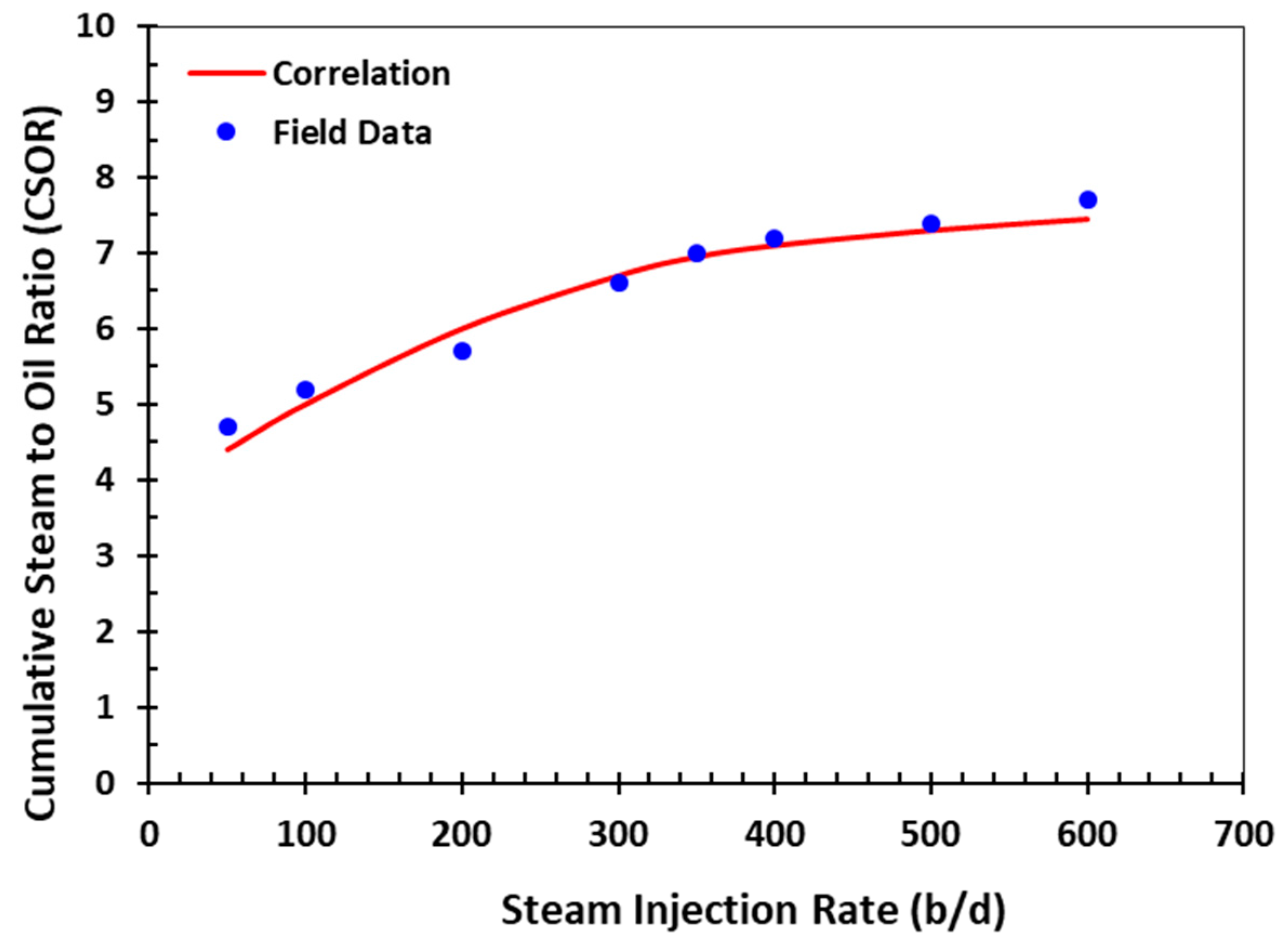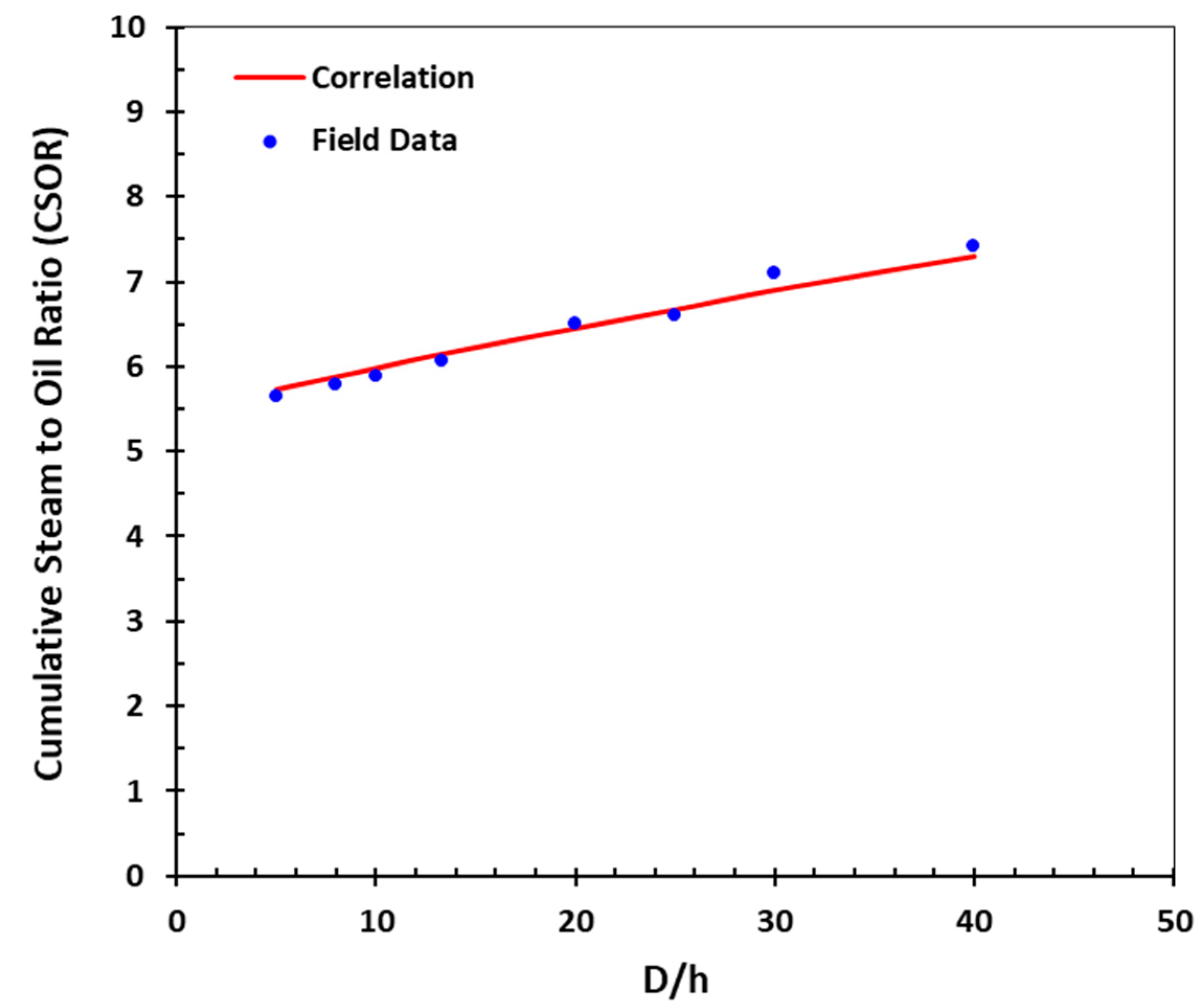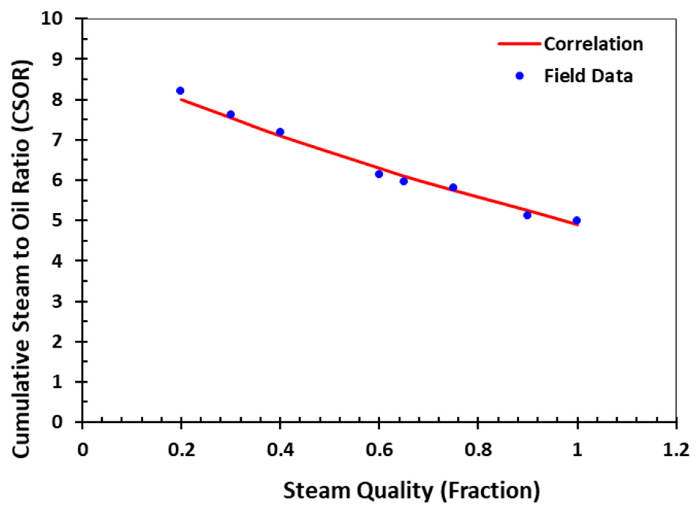Figure 2, Figure 3, Figure 4, Figure 5, Figure 6 and Figure 7 and Figure 12, Figure 13, Figure 14, Figure 15, Figure 16 and Figure 17 are obtained for the physical models with the same pattern (in shape and number of fractures) and the same dimensions in most cases. In addition, it is clear that all properties for steamflooding processes demonstrated on each figure except those on x and y-axes are the same when investigating effect of an independent variable on target functions. This conveys the message that these figures just present a limited volume of data used in this study to point out the important trends in performance of reservoirs during steamflooding according to a comprehensive parametric sensitivity analysis. 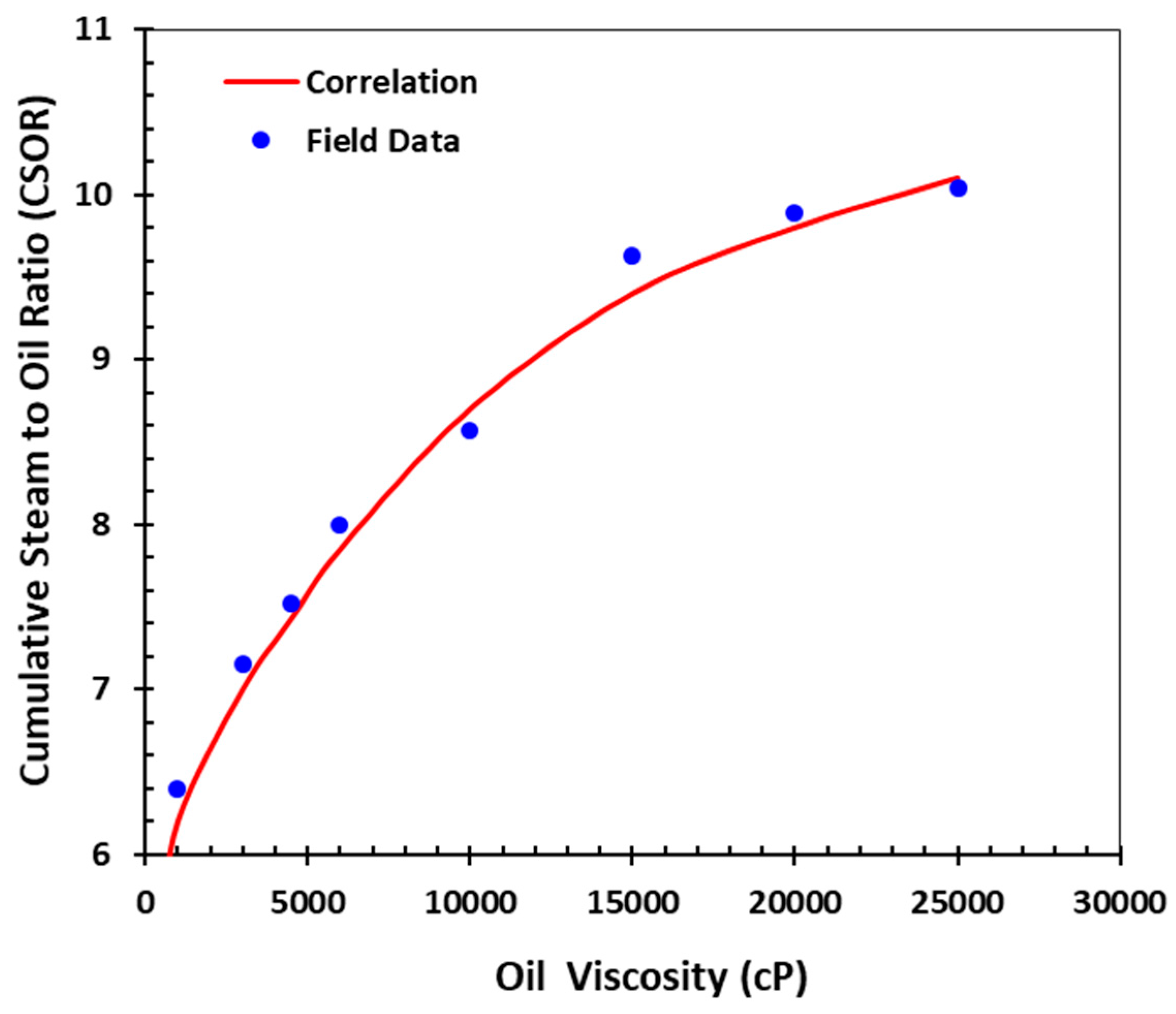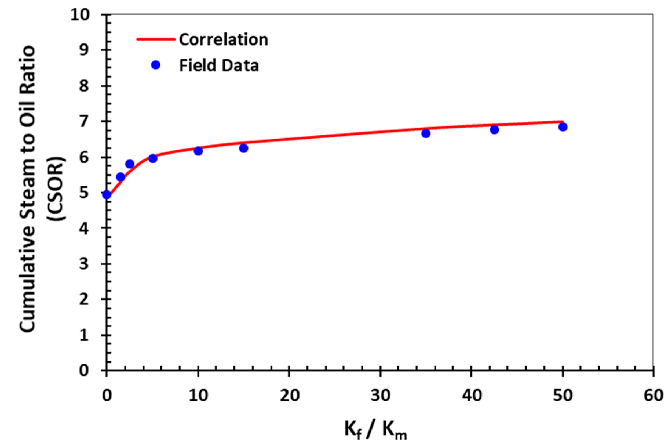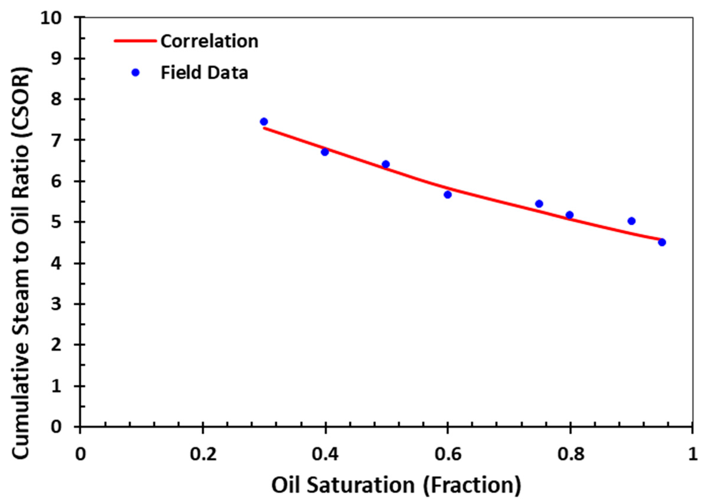Based on Figure 2, Figure 3, Figure 4, Figure 5, Figure 6 and Figure 7, CSOR increases with an increase in oil viscosity, steam injection rate, fracture to matrix permeability, and gross to net reservoir thickness. However, high steam quality and high initial oil saturation lead to reductions in CSOR, indicating better response to steam injection. 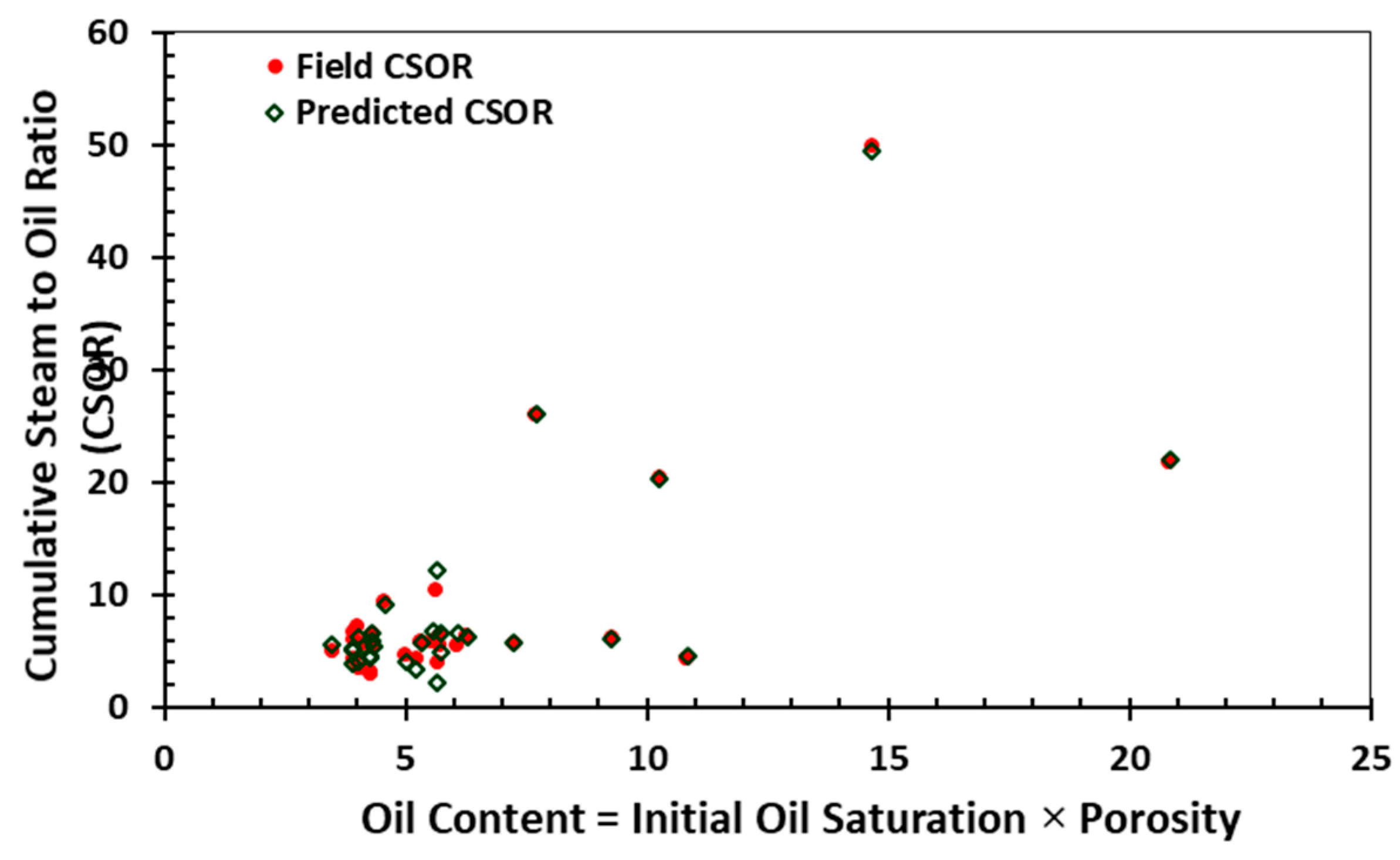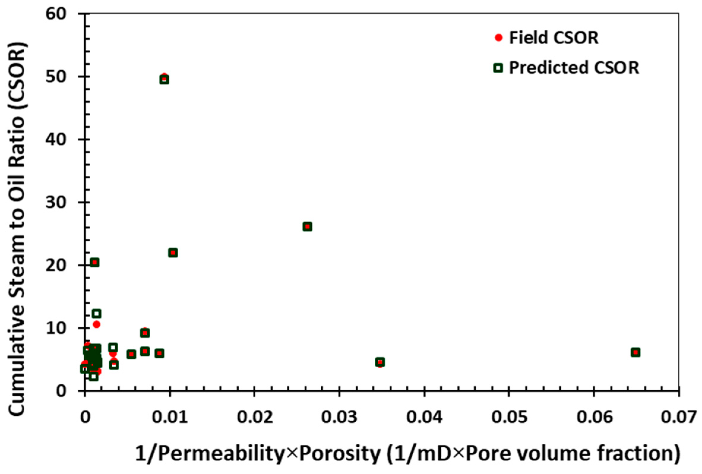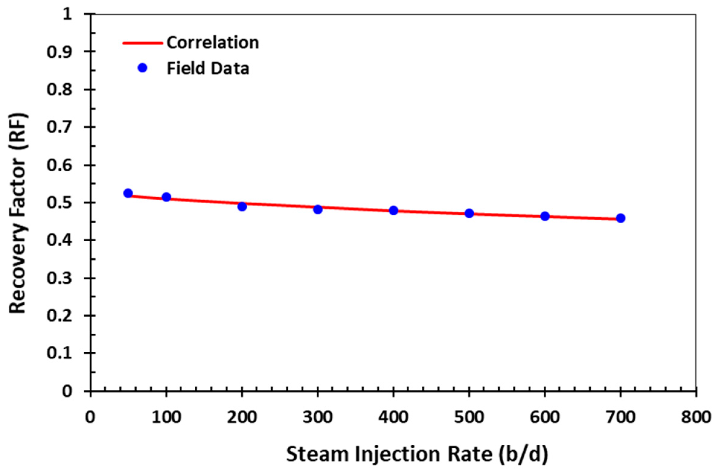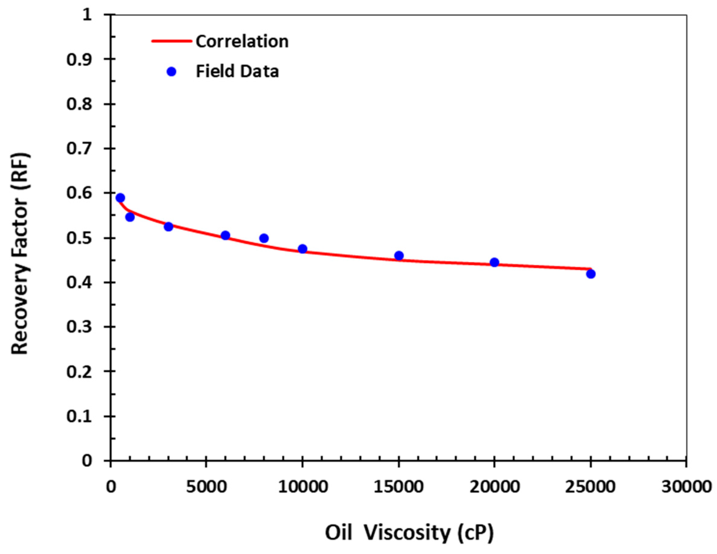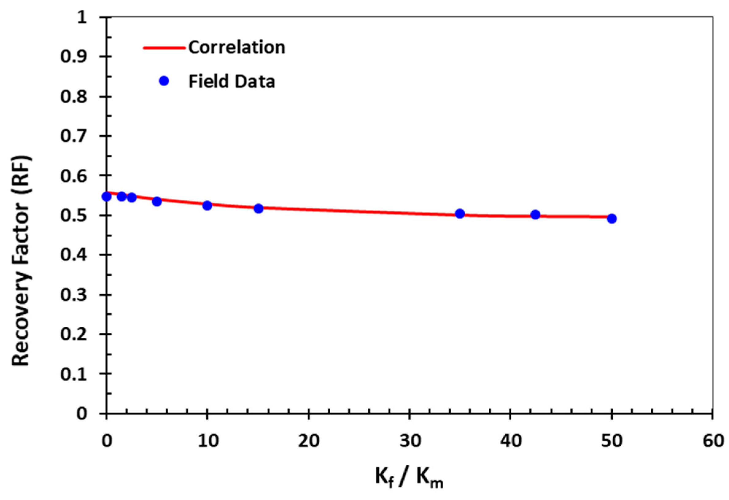In addition, Figure 2, Figure 3, Figure 4, Figure 5, Figure 6, Figure 7, Figure 8, Figure 9, Figure 10 and Figure 11 for CSOR indicate acceptable agreement between the field data and the predictions. It is clear that increase in steam injection rate improves the recovery rate but lowers the RF before steam breakthrough in fractured media (particularly highly fractured ones), as presented in Figure 12. Furthermore, if the reservoir contains oil with high viscosity, some areas can be bypassed during steamflooding, resulting in early breakthrough and consequently lower RF, as demonstrated in Figure 13. The same effect may occur when there are many fractures with high permeability in the reservoir (see Figure 14). Although the presence of fractures can cause an increase in the rate of oil production, a high density of fractures may have undesired effects on the overall performance of steamflooding, as depicted in Figure 14. 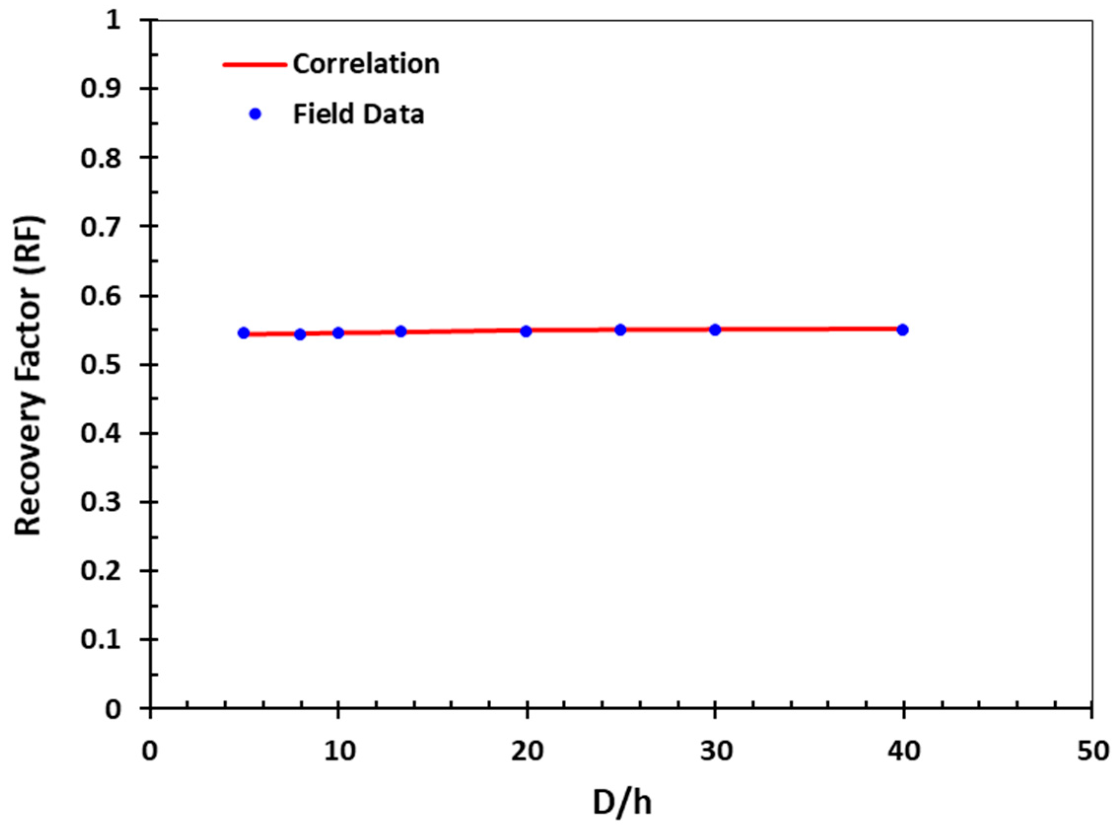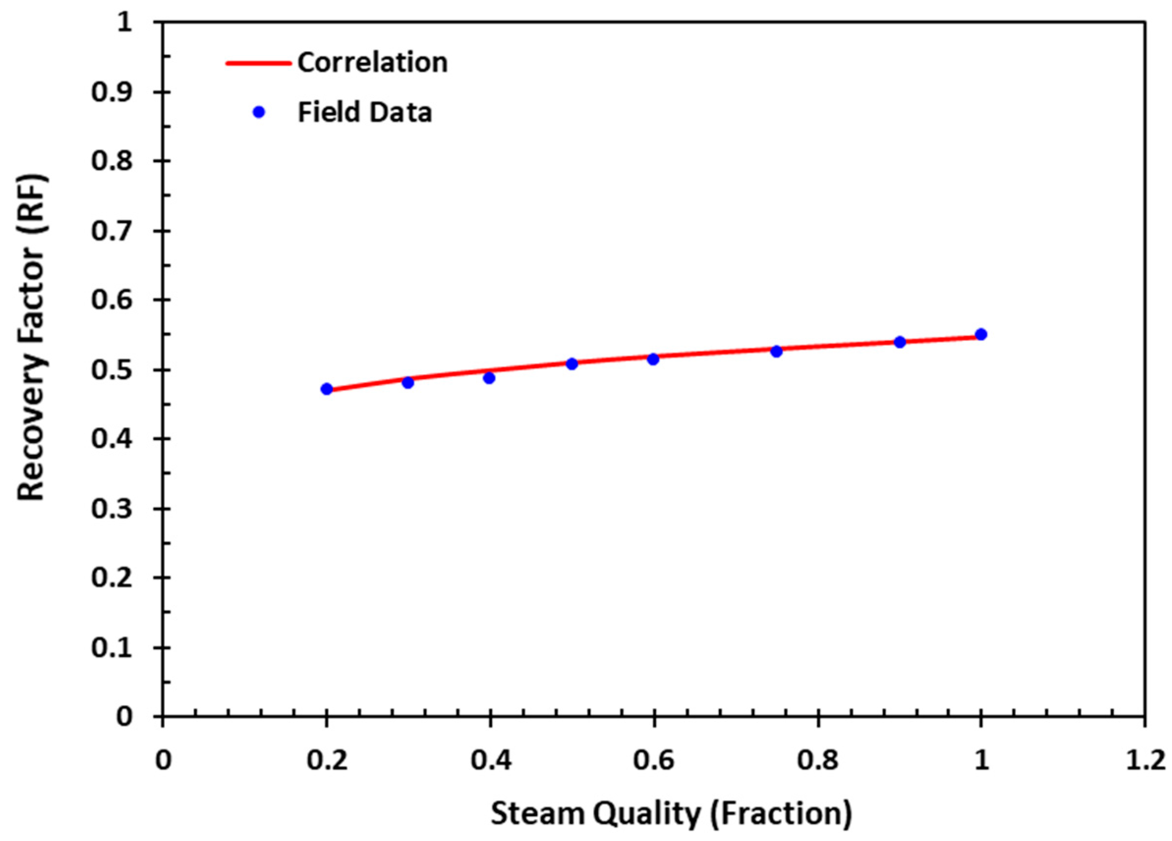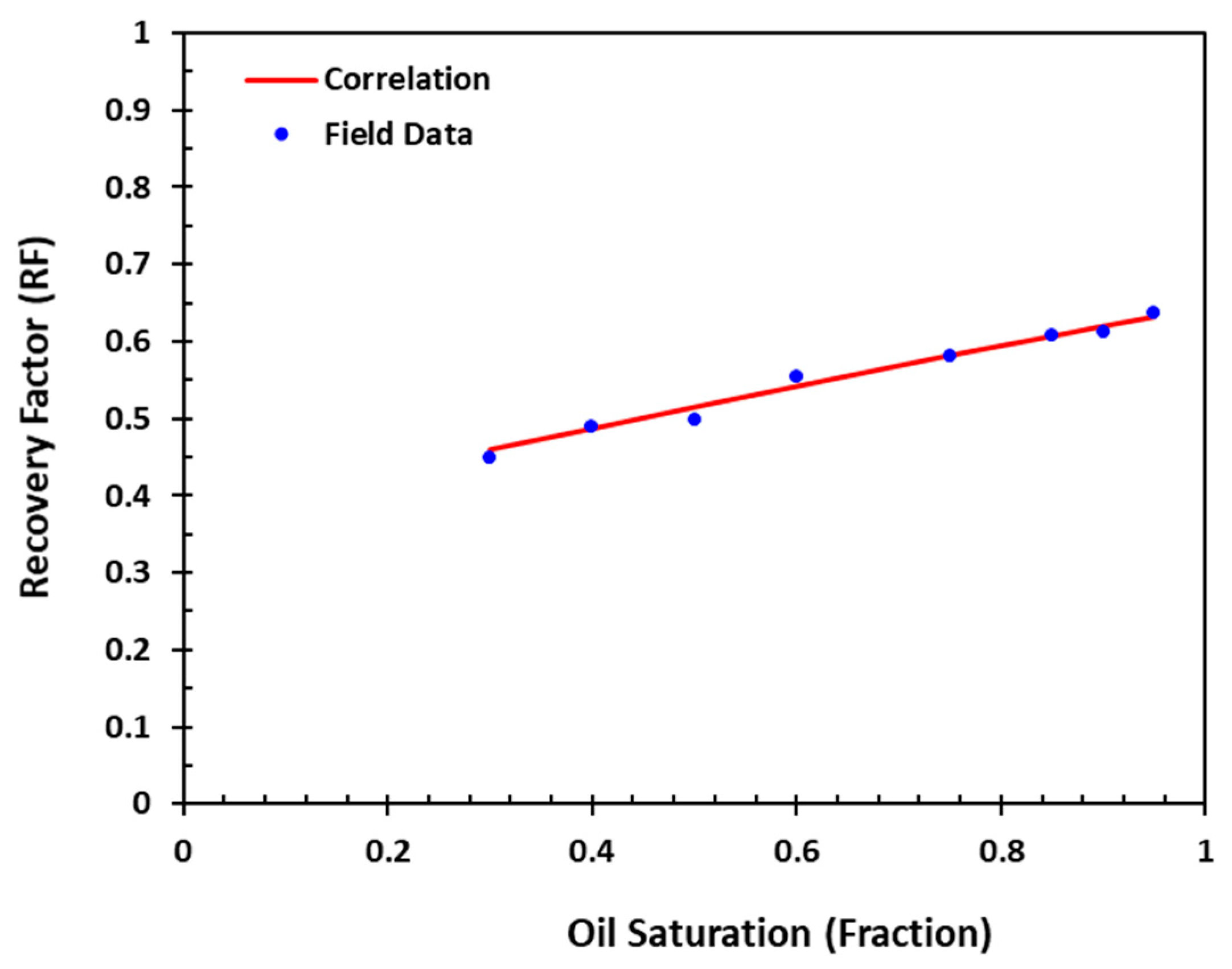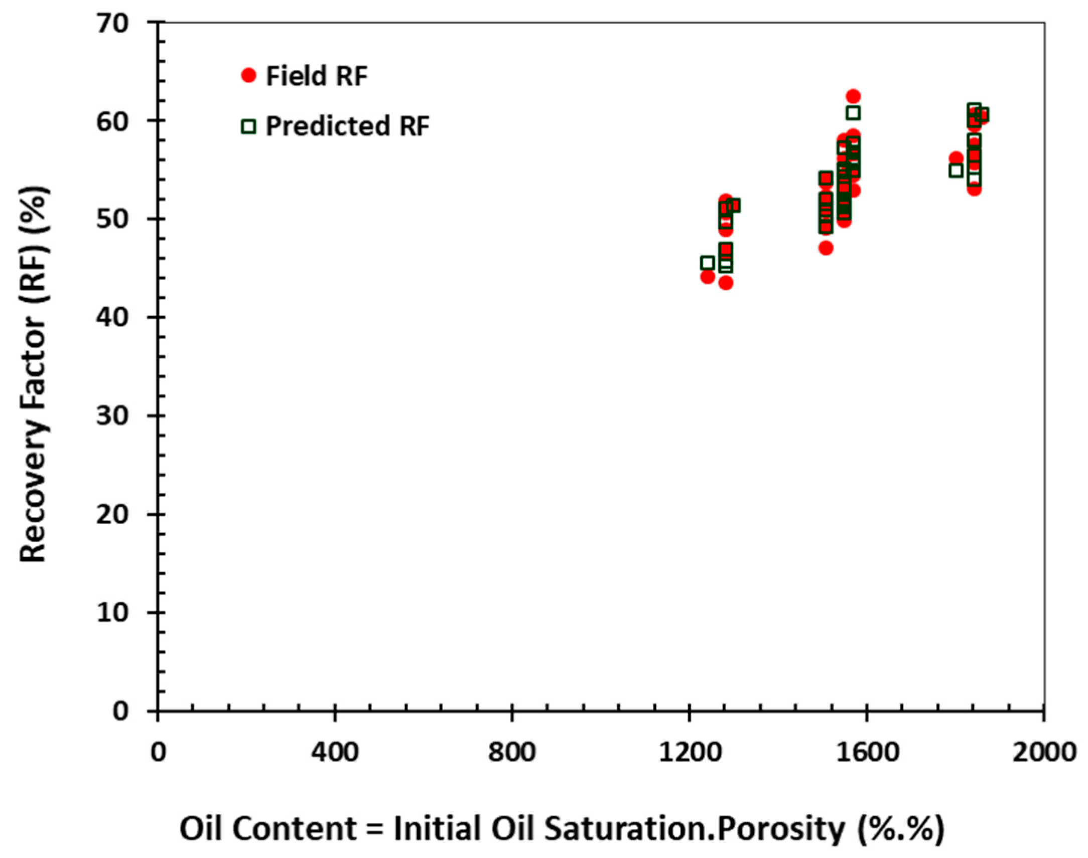Figure 15 shows that the ratio of the reservoir depth to the reservoir thickness does not have a noticeable impact on RF during steamflooding. As expected, steam quality and initial oil saturation have direct impacts on magnitude of RF. 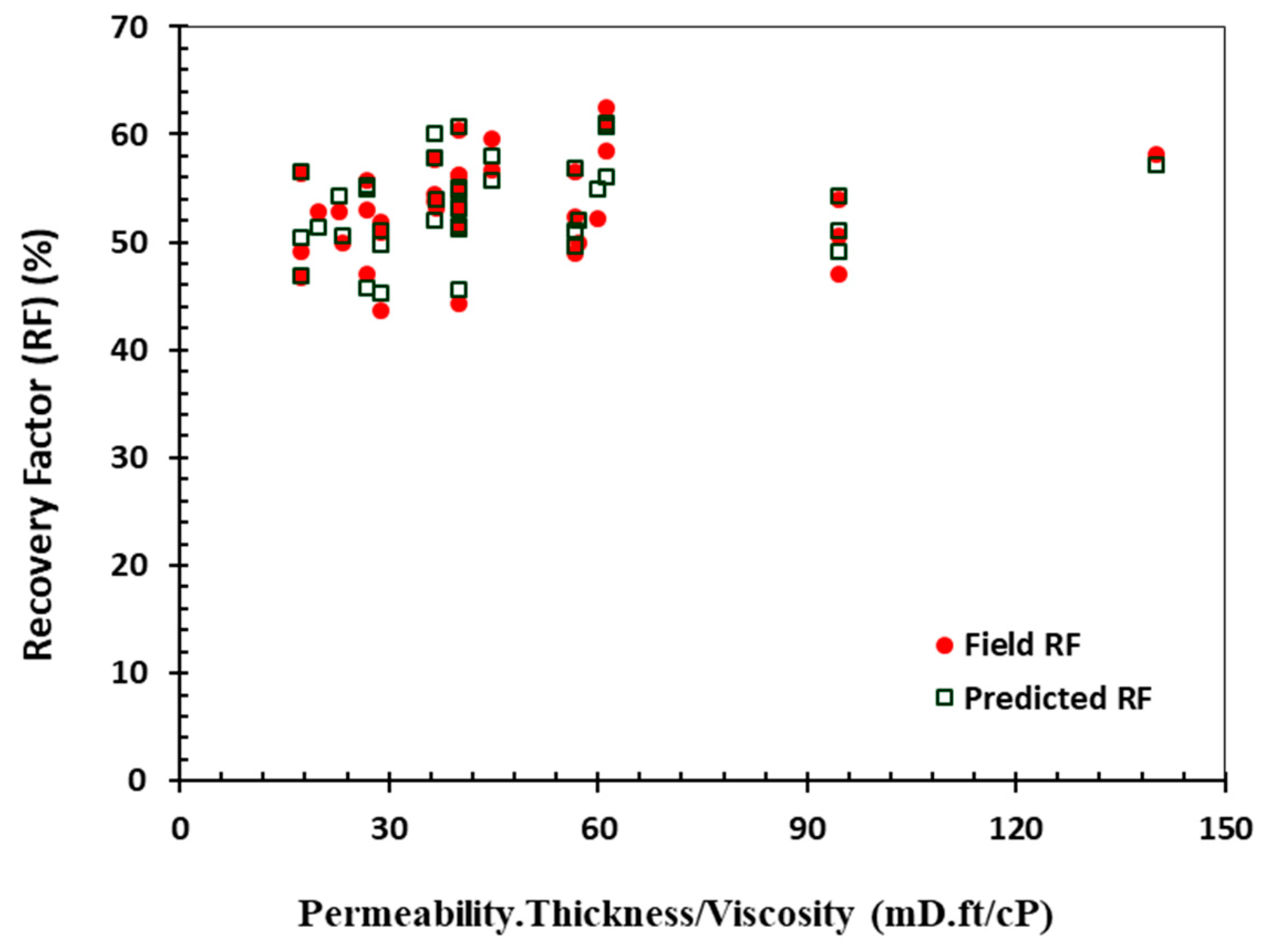Increase in these two parameters can improve the performance of the steamflood (see Figure 16 and Figure 17). Clearly, steam injection with higher quality steam enters more heat into the reservoir leading to an increase in temperature. Hence, it causes viscosity reduction that enhances the oil recovery. The figures related to RF again confirm the effectiveness of the statistical approach adopted in this study as a good match was observed between the field data and the results obtained from the correlations.

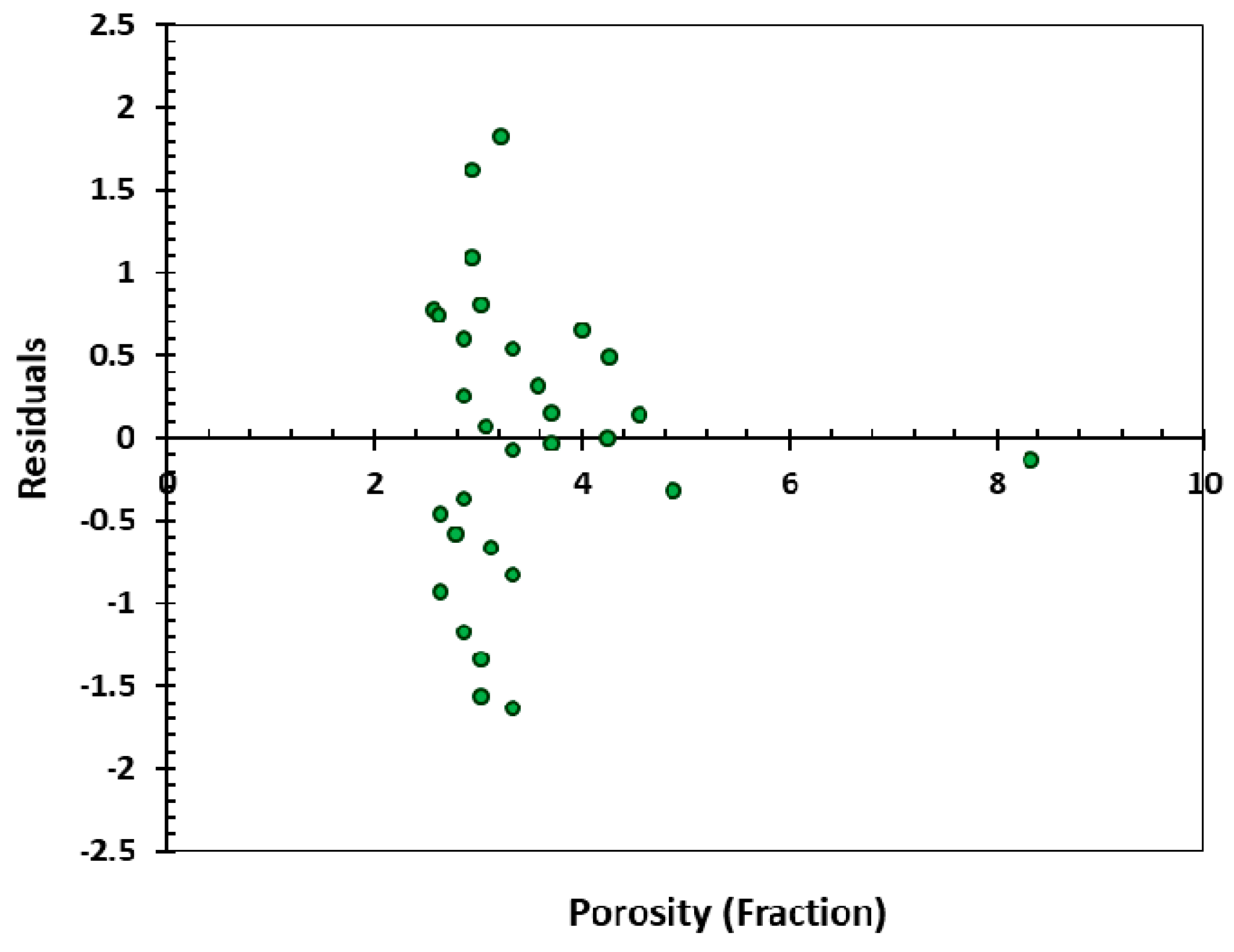
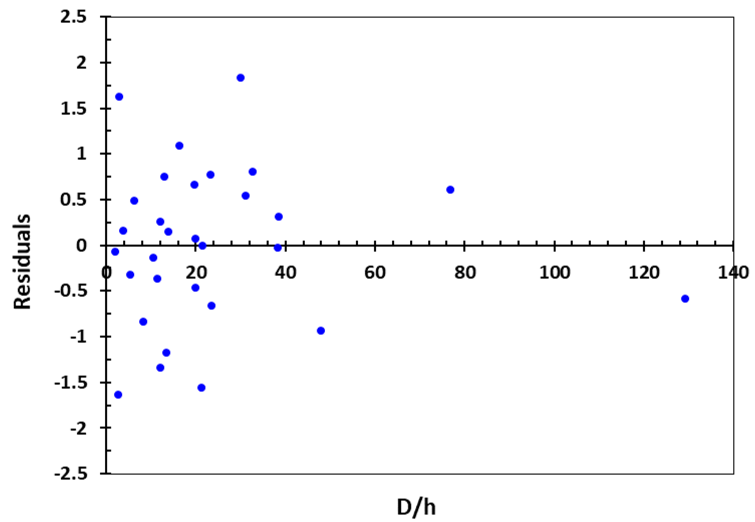
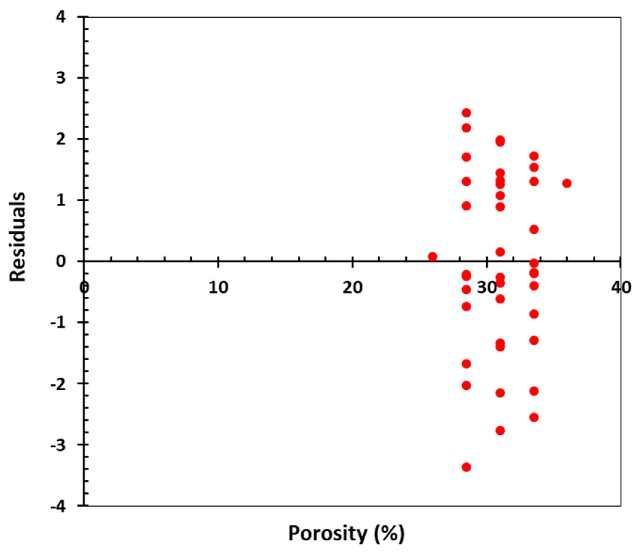
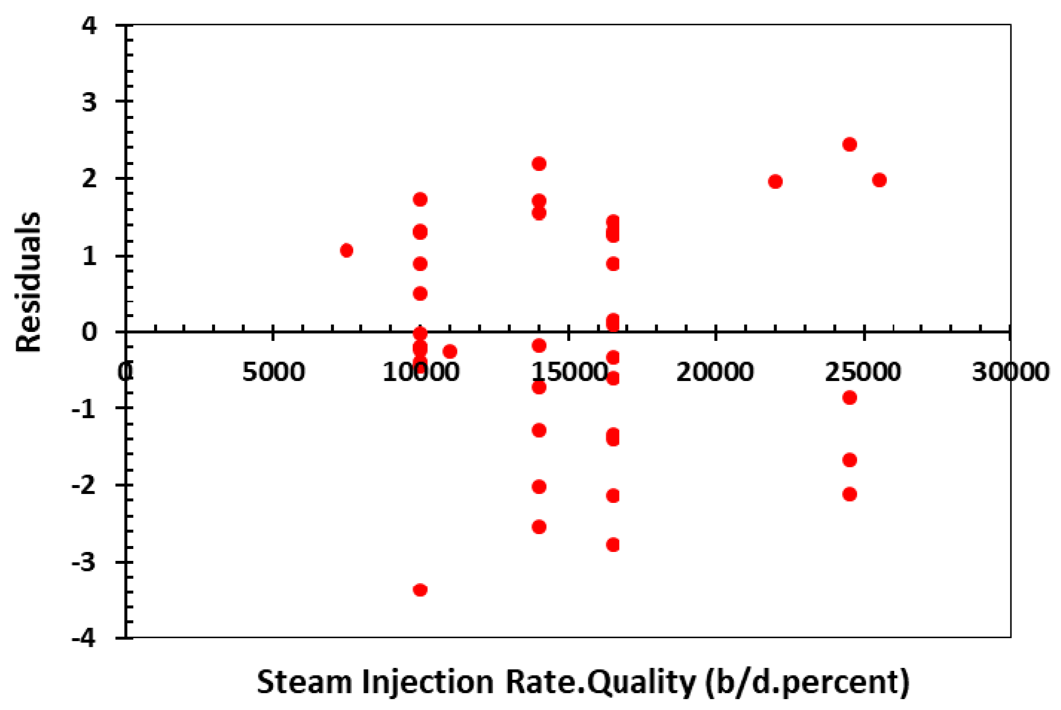
Figure 10 and Figure 11 are the residual plots for the CSOR with respect to porosity and a combined interaction component (including formation depth and thickness), respectively. In addition, residual plots for RF versus porosity and “steam quality multiplied by steam injection rate” are presented in Figure 20 and Figure 21, respectively, as two samples of the analysis of the residuals. For these four residual plots, the residual data shows random distribution all along the horizontal axis. In other words, the proposed linear regressions are valid for CSOR and RF in terms of the particular dependent variables shown on x-axis.

These results show that CSOR values for viscous oil extraction from NFCRs and some highly naturally fractured sandstone reservoirs can be correlated with reservoir and oil characteristics such as permeability, porosity, thickness, viscosity, and oil saturation. The following empirical relationship predictive function was developed in this study to estimate the CSOR during vertical well steamflooding in a NFCRs:

$$\begin{array}{l}\mathrm{CSOR}=a_0+a_{1}D+a_2\frac{1}{{\phi }_e}+a_3\frac{1}{K_m}+a_4{K}_f+a_5\frac{1}{{\mu }_o}+a_6\frac{1}{S_o}+a_7\frac{1}{q_s}+a_8{x}_s+a_9\frac{1}{S_o{\phi }_e}+a_{10}\frac{D}{h}+\\ a_{11}\frac{D}{h{\phi }_e{K}_m{\mu }_o{S}_o{q}_s}+a_{12}\frac{1}{{\phi }_e{q}_s}+a_{13}\frac{1}{{\phi }_e{K}_m}+a_{14}\frac{K_f}{K_m}\end{array}$$

(15)

Table 3 presents the values for the correlation coefficients, standard errors, and the ranges for the coefficients involved in the equation for the CSOR. Needless to mention that definitions of all parameters introduced in Table 3, Table 4 and

Table 5. ANOVA table for CSOR regression analysis.

Source	DF	SS	MS	F
Regression	14	2598.98	185.64	128.76
Residual	15	21.63	1.44	-
Total	29	2620.61	-	-

are presented in Section 4 of this paper. Since the variables such as K_m (mD), K_f (mD), (φ) porosity (%), S_o (%) have high magnitudes, their coefficients must be 4 to 6 digits significant while using regression correlations.

Recovery Factor (RF) is also an important asset assessment parameter, and a reliable tool to predict RF, even if only in a statistical manner, it would be valuable for first-order screening. Estimation of production performance is possible with initial and residual oil saturation data. The irreducible oil saturation is normally not known until the end of the thermal operation. Nevertheless, a correlation was established for RF prediction in terms of formation, steam, and oil properties considering the production history of some field pilots and laboratory tests data. To derive the following equation, a similar method as that for CSOR was implemented using statistical regression analysis:

$$\begin{array}{l}\mathrm{RF}=a_{15}+a_{16}{S}_o+a_{17}h+a_{18}{q}_{\mathrm{s}}+a_{19}{\phi }_e+a_{20}{K}_m+a_{21}{x}_s+a_{22}{\mu }_o+a_{23}\frac{K_{m}h}{{\mu }_o}+\\ a_{24}{S}_o{\phi }_e+a_{25}{q}_s{x}_s+a_{26}\frac{S_o{\phi }_{e}h{K}_m{q}_s}{{\mu }_o{x}_s}+a_{27}{q}_s{\phi }_e+a_{28}\frac{K_f}{K_m}\end{array}$$

(16)

The product of fracture permeability and matrix permeability and the interaction of all contributing parameters affect the RF in the form of “combinatory effects”. Table 4 contains data on the statistical correlation coefficients.

The corresponding ANOVA for CSOR is presented in Table 5. The F observed for CSOR (196.645) exceeds the critical value (2.31). Hence, all of the parameters considered in multivariable linear regression analysis of CSOR and their attributed effects are significant and cannot be ignored to simplify the statistical model.

There is a vigorous dependence between the objective function (RF) and the process variables implemented in the statistical analysis. This is evident considering the high values of the observed “F” compared with the tabulated critical value (

Table 6. ANOVA Table for RF during steamflooding.

Source	DF	SS	MS	F
Regression	13	657.68	50.59	70.60
Residual	27	19.34	0.72	-
Total	40	677.03	-	-

). It is also evident from Table 6 that the regression analysis for RF has an acceptable accuracy.

The magnitudes of the squared residuals (

Table 7. Summary of the Statistical Linear Regressions.

Objective Function	Multiple R	R2	Standard Error	Number of Observations
CSOR	0.97	0.96	0.01	30
RF	0.98	0.96	0.08	41

) can be used to check the accuracy of a linear regression. The results obtained in this research suggest a reasonable compatibility between the measured (field pilots and experimental data) and the forecasts (regression analysis). The proposed model and the associated curves can be implemented to forecast CSOR and RF in any given VO NFCRs given the limitations of the database.

Based on this study, the in situ oil viscosity and the initial oil saturation are the most significant factors influencing CSOR and RF. This was expected because of the nature of the steam processes.

According to the statistical information provided in Table 7 and

Table 8. Performances of previous predictive models and statistical correlations obtained in the current study.

Statistical Parameter	Chu [20]		Vogel [75]		Boberg [66]		Butler [67]		New Models
	RF	CSOR	RF	CSOR	RF	CSOR	RF	CSOR	RF	CSOR
R2	0.97	0.94	0.92	0.93	0.91	0.93	0.93	0.91	0.98	0.97
MSE	0.09	0.09	0.14	0.15	0.15	0.16	0.15	0.11	0.06	0.08
MIPE (%)	7.69	9.87	7.69	10.58	9.11	10.78	9.12	10.41	5.35	6
MAPE (%)	12.64	14.54	13.48	15.17	14.52	16	14.45	15.54	10.32	11.12

, there is an admissible match between the predicted and measured RF and CSOR. As shown in Table 8, the statistical parameters (e.g., R², minimum percentage error (MIPE), maximum percentage error (MAPE), and mean squared error (MSE)) for the new models obtained in this study and the relationships developed by other researchers such as Chu [20], Vogel [75], Boberg [66], and Butler [67] were obtained and compared. The statistical models developed, presented, and examined in this paper are more accurate in estimation of RF and CSOR as they appreciate from higher R² and lower MIPE, MAPE, and MSE.

The viscosity of cases analyzed ranges from 6 to 936 cP, thus the reservoirs are heavy oil reservoirs except for one medium heavy and one light oil reservoir in a NFR. The reservoir depth for the studied cases varies from 134 to 1350 m. This range covers the lower and upper limits of applicability of steamflooding. Matrix porosity and permeability vary from 0.12 to 0.35 and 1–4 D. In addition, the fracture “permeability” is between 1 and 1,000 D. These ranges represent an acceptable coverage for variation in parameters expected in such heterogeneous reservoirs despite small number of field pilots of steamflooding in NFCRs.

7.2. Screening of a Heavy Oil Field for Steamflooding

The Kuh-e-Mond heavy oil field, the largest on-shore heavy oil field in Iran, is a giant anticline located in the southwest of the country with a NW-SE trend. The field is 90 km long and 16 km wide with an estimated minimum heavy oil resource base of 10 × 10⁹ barrels OOIP. The heavy oil is found in three separate layers with depths ranging from 400 to 1,200 m and oil viscosities of 550 to 1120 cP in situ [78,79,80]. The trap structure formed during the main phase of Zagros folding in the late Miocene and Pliocene, as shown by the relatively constant thickness of the lower Miocene succession [78,79,80]. According to petrophysical evaluations, the Jahrum Formation limestone is a poor reservoir. Only part of it has a good porosity (φ) in the range of 0.24 to 0.31 and water saturation (S_w) around 0.20. This formation contains immobile heavy oil. The OOIP has been estimated at about 3 × 10⁹ barrels [78,79,80]. The Sarvak Formation, Cenomanian in geological age, is predominantly composed of intensely fractured marly limestone with some shale interbeds. The formation is divided into three main units in the study area: upper, middle, and lower units. The upper unit is composed of limestone with some weakly argillaceous impurities. Shale and marls are main rocks types in the middle Sarvak. Finally, the lower Sarvak predominantly consists of marly limestone with shale. Considering the intensely fractured nature of the Sarvak formation, heavy mud losses were reported during the drilling. The heavy oil resource in the Sarvak reservoir (OOIP) is estimated at 3.6 × 10⁹ barrels [78].

Lithostratigraphic information and fluid properties for the heavy oil reservoirs at the study area were collected, assessed, and summarized as presented in

Table 9. Reservoir and fluid properties of reservoirs at the Kuh-e-Mond heavy oil field.

Reservoir Abbreviation	Jahrum	Sarvak
Lithology	Dolomite and Dolomitic Limestone	Limestone
Depth (m)	680–900	1100–1200
Thickness (z) (m)	320	100
Net to Gross Ratio (%)	31	47
Net Pay Thickness (m)	99	47
Oil Viscosity (In situ) (cP)	1160	570
Temperature (T) (In situ) °F	70	110
Matrix Permeability (mD)	1	0.2–1.4
Fracture Permeability (mD)	300–500	350–500
Porosity (φ) (Fraction)	0.19	0.16
Oil Saturation (Fraction)	0.66	0.46

. In assembling this database, data from various sources such as drilling logs, geophysical logs, and field and laboratory test data were used. The average magnitudes of reservoir and fluid properties were determined for each reservoir using the available data. Single values reported for some properties of the reservoirs here are the average values of the reservoirs’ parameters; while, the properties may change with respect to the location within the field.

Based on the predictive regression models, if 200 to 250 b/d of steam with 80% to 90% quality is injected into the formation then CSOR and RF will be in the ranges of 6 to 7.2 and 41% to 49%, respectively, for the Jahrum HO reservoir. These ranges will be 6.3 to 8 and 37% to 44% for CSOR and RF in Sarvak HO reservoir. The screening results imply that Jahrum reservoir is technically recoverable by using steamflooding despite an average rock matrix porosity of 19%. This is mainly because of other commendatory factors such as depth, thick net pay, and relatively high oil saturation. The Sarvak reservoir met the technical screening criteria but the Jahrum reservoir is considered a moderately better candidate. Very low matrix permeability and low oil saturation (<50% PV) lead to lower RF and higher CSOR in the Sarvak reservoir. However, under current economic conditions, HO exploitation from these reservoirs remains economically unattractive.

We examined the developed correlations for estimation of CSOR and RF in oil sands and unconsolidated heavy oil sandstone reservoirs and compared the results with the CSOR estimations predicted by a correlation proposed by Chu [20]. The results suggest that the new correlations also can be used reliably to estimate CSOR and RF in oil sands and unconsolidated heavy oil sandstone reservoirs. The developed correlations can be considered a general from of correlations to be utilized for wide ranges of reservoir properties from NFCRs to oil sands and unconsolidated heavy oil sandstone reservoirs.

During utilization of steam injection in any given heavy oil reservoir, laboratory experiments and field interposition can serve the operator to avoid or rectify high CSOR by selecting an appropriate production rate and/or steam injection rate. The recovery and injection rates affect thermodynamic conditions, steam/oil ratio, and composition of the liquid phase, which is mobilized and moving to the production well. Hence, utilizing experiments and statistical modeling (i.e., using different flow rates as various dynamic conditions) which is much inexpensive and yet faster compared with field trials will be definitely beneficial in systematic assessment of the performance of steamflooding in any given HO NFCR. Estimation of vital process performance indicators such as CSOR and RF can provide invaluable directions for optimum design of a recovery technology in terms of flow rate and thermodynamic status of the fluids. Furthermore, accurate prediction of RF and CSOR for a given HO NFCR can enable process engineers with reasonable rules of thumb to minimize heat loss, which can lead to notable steam condensation in the reservoir.

7.3. Limitations and Assumptions for the Correlations of CSOR and RF

Table 10. Range of variables to estimate RF and CSOR.

	Parameter	Min	Max
Input	Depth (m)	134	1350
	Matrix porosity (Fraction)	0.12	0.35
	Matrix permeability (mD)	1	400
	Fracture permeability (D)	1	1000
	Oil viscosity (cP)	6	936
	Initial oil saturation (Fraction)	0.3	0.9
	Steam quality	0.3	1
Output	Recovery factor, RF, (Fraction)	0.4	0.7
	Cumulative steam oil ratio (CSOR)	3.0	10.0

presents the range of variables contributed in the correlations developed to forecast of RF and CSOR in NFCRs.

We have identified and acknowledged the following sets of limitations for the proposed statistical models. However, in practice they remain as appropriate and accurate predictive tools:

(1)

Porous medium is non-deformable (constant porosity assumption).

(2)

For mass, there is no source term except for the steam.

(3)

A majority of the experimental data used in this research study have been obtained from the experiments in two-dimensional (2-D) porous systems.

(4)

The correlations are only valid in the range of parameters used in the current study. Ranges of fluid and porous media properties in oil fields are almost the same as in the experimental studies considered in this statistical investigation.

(5)

The Darcy law is valid throughout the EOR process. Flow in porous media is mostly laminar (i.e., Re < 1) during steamflooding.

(6)

RF and CSOR forecasts are not affected greatly by the geometry of the physical models (experimental data taken from the literature) used in the experimental works (taken from the literature). It only influences the residual oil saturation, moderately. This is because the geometry dominates the shape of the corners and the end points in a porous system. In addition, in these experiments no changes was observed for a high capillary threshold and permeability with regard to geometry variations in the porous system.

(7)

There were a certain number of porous media with specific fracture patterns selected for this statistical study. The proposed statistical models are very accurate for these fracture configurations. Thus, the only major limitation here is the type of fracture configuration. Nevertheless, if the effective fracture permeability is known for a porous system with unknown fracture configuration then the developed statistical models can be used to forecast the RF and CSOR with an acceptable accuracy.

Steamflooding and its variants utilizing either vertical, inclined, or horizontal wells can be used for any type of reservoirs regardless of the reservoir rock type if the oil viscosity is less than 5000 cP. This also includes conventional reservoirs containing light oil. In this case, steam and the resultant heat in the reservoir serve as stimulant rather than sweeping the oil or lowering down the oil viscosity (the well-known piston model). The only exception would be highly porous rocks such as diatomite and chalk which are also structurally very weak when exposed to heat [81,82]. In addition, the correlations introduced in this paper can be used to assess the performance of steamflooding in non-fractured reservoirs, as well. In fact, both fractured and non-fractured media are considered in the correlations and in the case of non-fractured media where there is no natural fractures, those parameters will be cancelled from the equations and the remaining terms can be used to evaluate the performance of the process in non-fractured systems (single porosity systems). The proposed correlations can be used as a proxy to assess the feasibility of the process in the candidate reservoirs. However, CSOR is a strong indicator of economic feasibility of any thermal operations under the current economic climate. For example, in Canada any thermal operations with CSORs below 3 are considered economic. Considering decades of experience in thermal operations in Canada especially for well-known and commercialised technologies such as SAGD and HCS, wealth of available field data, and advanced process optimization practices, the CSOR is now down to less than 2. Considering the case study presented here, this heavy oil field is a poor candidate for steamflooding. However, utilizing long horizontal wells will increase the oil recovery and will reduce the CSOR in the case studied. In addition, adopting cyclic steam stimulation processes can reduce the steam requirements, lower down the CSOR, and increase the RF and oil production rate. Nevertheless, the correlations developed and presented here can only be used for estimation of RF and CSOR in thermal heavy oil operations utilizing vertical wells. Clearly, new sets of correlations or models will be needed to predict performance of steam processes utilizing horizontal wells. Such projects still do not exist (therefore no filed data is available at the moment) when it comes to carbonate reservoirs. Some steam injection variants such as HCS process are being tried in bitumen saturated Devonian carbonates in Alberta, Canada.

8. Conclusions

This article presents new statistical models to forecast cumulative steam to oil ratio (CSOR) and recovery factor (RF) in naturally fractured reservoirs under steamflooding. The CSOR and RF were statistically correlated in terms of physical properties of the oil, reservoir fluid and rock properties, and steam properties. The following conclusions seem reasonable, despite a modest database:

(1)

The correlations developed in this study are derived from data obtained from field and laboratory tests. High correlation coefficients (R²) show that the multivariable regression method used is a strong predictor of the economic assessment factors CSOR and RF.

(2)

The errors involved in even the worst cases were less than 10%, giving confidence that first-order economic decisions can be made with these relationships.

(3)

The parameters considered for regression analysis are not able to forecast the oil production characteristics of steamflooding in NFCRs if they are used alone. Combination terms for the main variables were used that led to a reliable outcome.

(4)

Initial oil saturation and oil viscosity have the greatest impact on predictor models for CSOR and RF. Nevertheless, all of the chosen parameters have a significant influence on the predictions. Therefore, none of them should be abandoned in the search for a simpler model.

(5)

Comparison of statistical correlations developed in this paper, and the previous correlations shows that the newly defined equations can predict steamflooding efficiency in heavy oil NFCRs with high accuracy such that the maximum error percentage is lower than 12% for the equations obtained in this study.

(6)

The proposed correlations were applied to predict CSOR and RF in two fractured heavy oil reservoirs, with apparently good results. This supports the use of these relationships for initial technical feasibility assessment of VO NFCRs for vertical well steamflooding.