Economic Optimal HVAC Design for Hybrid GEOTABS Buildings and CO2 Emissions Analysis

1
Department of Mechanical Engineering, University of Leuven (KU Leuven), Celestijnenlaan 300-box 2421, 3001 Leuven, Belgium
2
EnergyVille, Thor Park 8310, 3600 Genk, Belgium
*
Author to whom correspondence should be addressed.
Energies 2018, 11(2), 314; https://doi.org/10.3390/en11020314
Submission received: 21 December 2017
/
Revised: 14 January 2018
/
Accepted: 19 January 2018
/
Published: 1 February 2018
(This article belongs to the Special Issue Geothermal Heating and Cooling)
Abstract
:In the early design phase of a building, the task of the Heating, Ventilation and Air Conditioning (HVAC) engineer is to propose an appropriate HVAC system for a given building. This system should provide thermal comfort to the building occupants at all time, meet the building owner’s specific requirements, and have minimal investment, running, maintenance and replacement costs (i.e., the total cost) and energy use or environmental impact. Calculating these different aspects is highly time-consuming and the HVAC engineer will therefore only be able to compare a (very) limited number of alternatives leading to suboptimal designs. This study presents therefore a Python tool that automates the generation of all possible scenarios for given thermal power profiles and energy load and a given database of HVAC components. The tool sizes each scenario properly, computes its present total cost (PC) and the total CO emissions associated with the building energy use. Finally, the different scenarios can be searched and classified to pick the most appropriate scenario. The tool uses static calculations based on standards, manufacturer data and basic assumptions similar to those made by engineers in the early design phase. The current version of the tool is further focused on hybrid GEOTABS building, which combines a GEOthermal heat pump with a Thermally Activated System (TABS). It should further be noted that the tool optimizes the HVAC system but not the building envelope, while, ideally, both should be simultaneously optimized.
1. Introduction
In the early design phase, a design engineer will typically firstly estimate the energy profile necessary to heat and cool the future building based on a few parameters such as the building conditioned volume, its floor surface area, the type of occupancy, its windows-to-wall ratio, whether the structure is light or heavy, and typical weather conditions at the given location. Based on the energy profile and optionally some additional constraints set by the client, the design engineer will then propose a combination of properly sized heat and cold production and emission systems (further referred to as the Heating, Ventilation and Air-Conditioning (HVAC) scenario) able to deliver the required powers and energy loads. Finally, the investment, running, maintenance and replacement costs can be estimated along with the total CO emission or another indicator for environmental impact. Ideally, several alternative HVAC scenarios are compared with each other to choose the most appropriate one. However, since the presented work flow is highly time-consuming, the number of considered alternative scenarios remains (very) limited leading to suboptimal designs. This work presents therefore a Python tool that automates the generation of all possible scenarios for given thermal power profiles and energy load and a given database of HVAC components. The tool further sizes each scenario properly, computes its present cost (PC) based on the investment, running, maintenance and replacement costs, and the total CO emission associated to the building energy use. Finally, the different scenarios can be searched and classified to pick to the most appropriate scenario. The tool is based on static calculations based on standards, manufacturer data and basic assumptions similar to those made by engineers in the early design phase. It should further be noted that the tool optimizes the HVAC system but not the building envelope while, ideally, both should be simultaneously optimized.
This paper is structured as follows. Firstly, Section 2 describes common methods used to improve or optimize HVAC systems of buildings. Secondly, Section 3 introduces the methodology proposed in this work, Section 4 clarifies its assumptions, and Section 5 lists the considered HVAC components and summarizes their characteristics. Finally, Section 6 compares the Present Cost (PC) and the CO emissions of conventional, (pure) GEOTABS, and economic optimal HVAC designs for different boundary conditions, and Section 7 concludes and proposes some further improvements.
2. Existing Methods
In Europe, buildings are responsible for 40% of the total energy use from which half is used for heating and cooling [1]. In accordance to the European Union’s Directive 2010/31/EN [2], the energy requirements for buildings are becoming increasingly stringent. Not only should the buildings become more energetically efficient through a better design of the building envelope (insulation, shading, etc.) and the use of more efficient HVAC devices, but buildings are also obliged to use a minimum of renewable energy sources. Both requirements put building designers and installers under pressure to be innovative and up-to-date with the various and rapidly improving available technologies. Furthermore, systems are becoming increasingly complex. Where a standard gas- or oil-fired boiler and a compression cooling machine connected to radiators and ventilation units used to be installed everywhere, buildings using a combination of production systems such as gas boilers, heat pumps, etc., emission systems such as radiators, fan coil units, chilled beams, TABS, etc., and additional renewable energy sources such as photovoltaic panels, solar boilers, borefields, etc. are becoming common in Europe. With this increase in system complexity and the lack of knowledge about these new and rapidly improving technologies, design tools are becoming highly necessary to help designers and installers to optimize both the design and the control of buildings. According to Ellis and Mathews (2002) [3], researchers believe that design tools based on an integrated approach where the system efficiency is optimized taking the interactions between the various factors and their constraints into account could lead to savings around 70%.
According to the American Society of Heating, Refrigerating and Air-Conditioning Engineers (ASHRAE), three types of equipment related programs exist to help HVAC designers: (i) electronic catalogues that simply list available components respecting given constraints, (ii) equipment optimizers that propose a range of possible equipment alternatives for given design criteria, and (iii) equipment simulation programs that can take the interactions and constraints of different devices connected to each other into account [3]. While only equipment simulation programs can truly help the design engineer to optimize the system, such a tool is confronted to an intricate problem. Firstly, the number of design variables (type, size and combination of systems) is usually very high. Secondly, the operation efficiency of each system is very dependent on its components and how they interact, and, finally, the design is heavily based on the building’s energy demand, which is difficult to predict in the early design phase.
In the literature, building and HVAC designs are typically optimized by heuristic methods such as genetic algorithms. Due to their slow convergence, generally only a limited number of parameters are optimized while the control is fixed or optimized over a short period of time. Another popular approach is to formulate the optimal design problem as a mixed integer linear programming (MILP) problem, allowing many variables to be solved in a reasonable computing time. However, a MILP formulation requires linear models that prevents its use in simulation based building design optimization. Nguyen et al. [4] provide an extensive literature study on building optimization. Examples of optimization using genetic algorithms can be found in e.g., Ooka and Komamura (2009) [5], who used a genetic algorithm to optimize the equipment capacity and operation planning of buildings, and, in Seo et al. (2014) [6], who used a multi-island genetic algorithm to optimize the HVAC system of apartments. The MILP approach has been used by, e.g., Ashouri et al. [7] to simultaneously optimize HVAC equipment, sizing and operation, and by Patteeuw and Helsen [8], who developed a similar method but also included multiple temperature levels to represent energy storage and conversion efficiencies in a more realistic way, and the explicit modelling of the electricity generation side. Heuristic and MILP optimization methods can also be combined. Evins [9] simultaneously optimized the building envelope of an office building, its HVAC, and its control, using a multi-objective, multi-level optimization scheme. At the top level, a genetic algorithm optimizes some building envelope parameters and the choice and size of the HVAC system by running an EnergyPlus model. At the lower level, a MILP algorithm is used to optimally control the HVAC with minimization of the running cost as objective. Due to the huge problem formulation, the author used a combination of a workstation with twin eight-core processors and 64 Gb RAM and additional 960 computing cores each with 4 Gb RAM to solve the MILP problems in parallel.
On the more practical and political sides, EU’s Directive 2010/31/EN compels the EU countries to limit the energy used by the building sector but leaves each country the freedom to develop its own legislative framework to reach the energy goals. In Belgium, a software called EPB (in Dutch and PEB in French) (version 9.0.0, Vlaamse energieagentschap (VEA), Belgium) is used to compute an energy level indicator. The energy level is evaluated based on quasi static energy loss computations and on a point table to grade different HVAC systems. The Flemisch Energy Agency (VEA) publishes every second year a report that investigates for which energy level the building would also be cost optimal with respect to the sum of the investment, running and replacement costs [10]. While the results are very instructive for decision makers of Flanders, the method is not practical for designers as it is difficult to relate the energy indicator to real energy use and the designer is restricted to the initial assumptions made by the program. Furthermore, the EPB software is not able to calculate dynamic aspects, system integration and control correctly.
The drawback of the presented methods is that they require intensive computer power, specialized software, and intensive modelling and set up work. The results are further difficult to analyse as they are influenced by numerous optimization parameters and assumptions/approximations made by the tools. Therefore, this work proposes to go back to the straightforward, but time-consuming method used by engineering offices and to automate it. The method should be based on a limited set of parameters, and it should remain intuitive to be usable in the early design phase. The starting point of the method is the heating and the cooling load duration curves (LDC) of the building, which represent the thermal powers required to condition the building. The thermal powers are furthermore ordered and each power is plotted with a width equal to the sum of hours that it is used, such that the integral of the LDC represents the yearly energy load of the building. The developed method proposes then all possible HVAC scenarios composed of the devices present in the database, which can provide the powers and the energy load of the LDC and computes the scenarios PC (including the investment, running, maintenance and replacement costs) and CO emissions (see Section 3). The method has the main advantage to automatically generate and size, and to return the necessary information about each possible HVAC scenario such that design engineers can make the optimal choice, while the method complexity is sufficiently low such that the results can be easily manually verified.
It should be noted that optimizing building and HVAC designs goes hand in hand with its control. For example, GEOTABS buildings can be energetically very efficient, but they are difficult to control due to the slow reaction of TABS [11,12,13,14,15] and their potentially conflicting behaviour with the fast reacting emission systems such as ventilation, radiators, etc. [16,17,18]. While this control aspect is beyond the scope of the paper, readers interested in (optimal) control of GEOTABS buildings are referred to [12,19,20,21,22,23] for rule-based controllers and to [24,25,26,27,28,29,30,31]) for optimal control.
3. Methodology
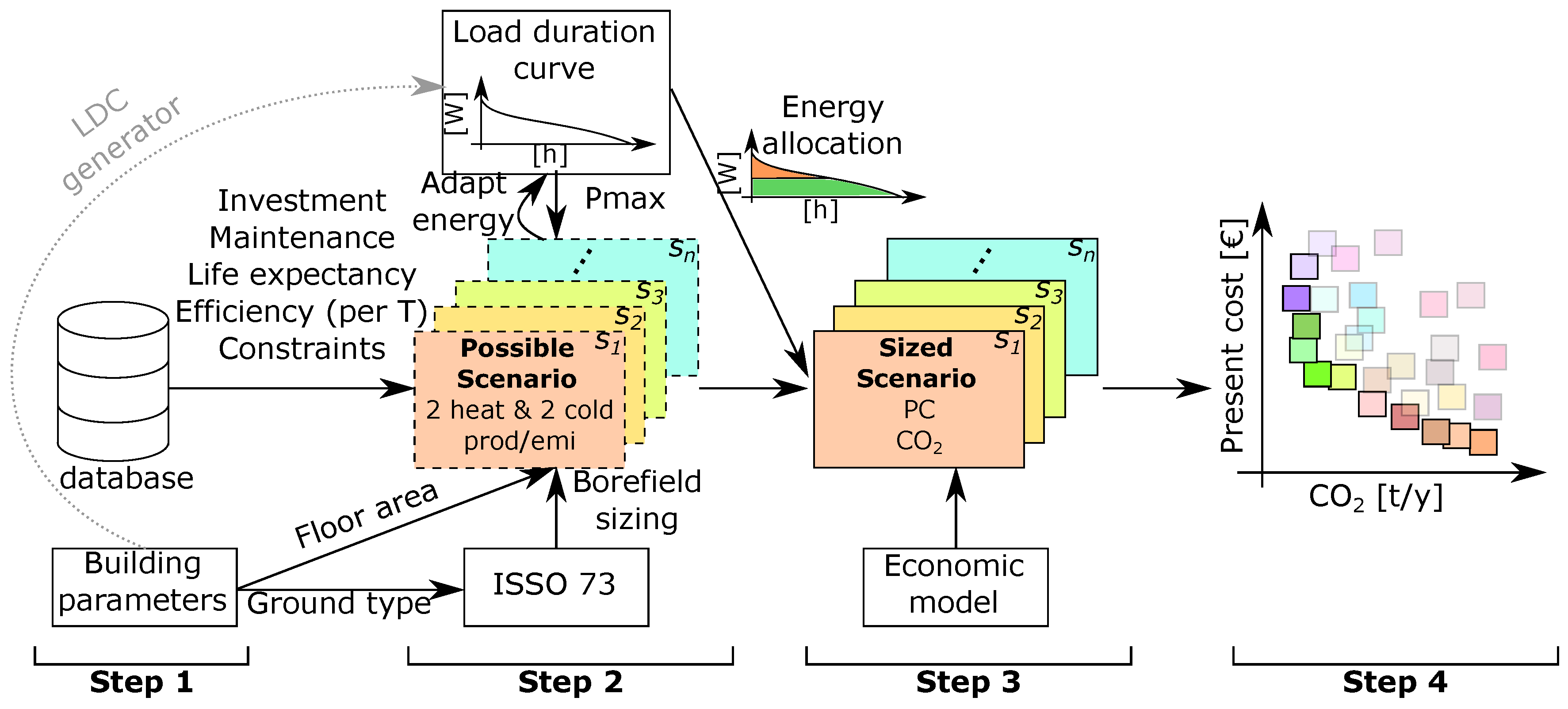
The methodology used by the developed tool to optimize the HVAC system for a given building is schematically represented in Figure 1, which shows the four steps that are consecutively carried out.
Step 1: Gather building and components data
Firstly, a database of HVAC components is created containing for each component (see Section 5): its cost function returning its price as a function of its size (kW, m, etc.), its maintenance cost, and its life expectancy (see Table 1 and Figure 3). If the component is a production device, the energy efficiency is given for different temperatures (for heat production: 30, 45, 60 C, and for cold production: 10, 15, 20 C, see Table 2) and if the component is an emission device, its nominal supply and return temperatures are specified (see Table 3). The database also contains the component constraints (e.g., ground source passive cooling (GSPC) cannot deliver water colder than 15 C). Additionally, a number of building parameters are required such as its total floor area (used to size the Concrete Core Activation (CCA) system) and the ground characteristics that influence the borefield design. In its final state, the tool should also be able to estimate the energy profile of the building based on its parameters in the form of load duration curves (LDC). However, this is not yet implemented and the building’s LDCs are thus now assumed to be given.
Step 2: Generate and size all possible HVAC scenarios
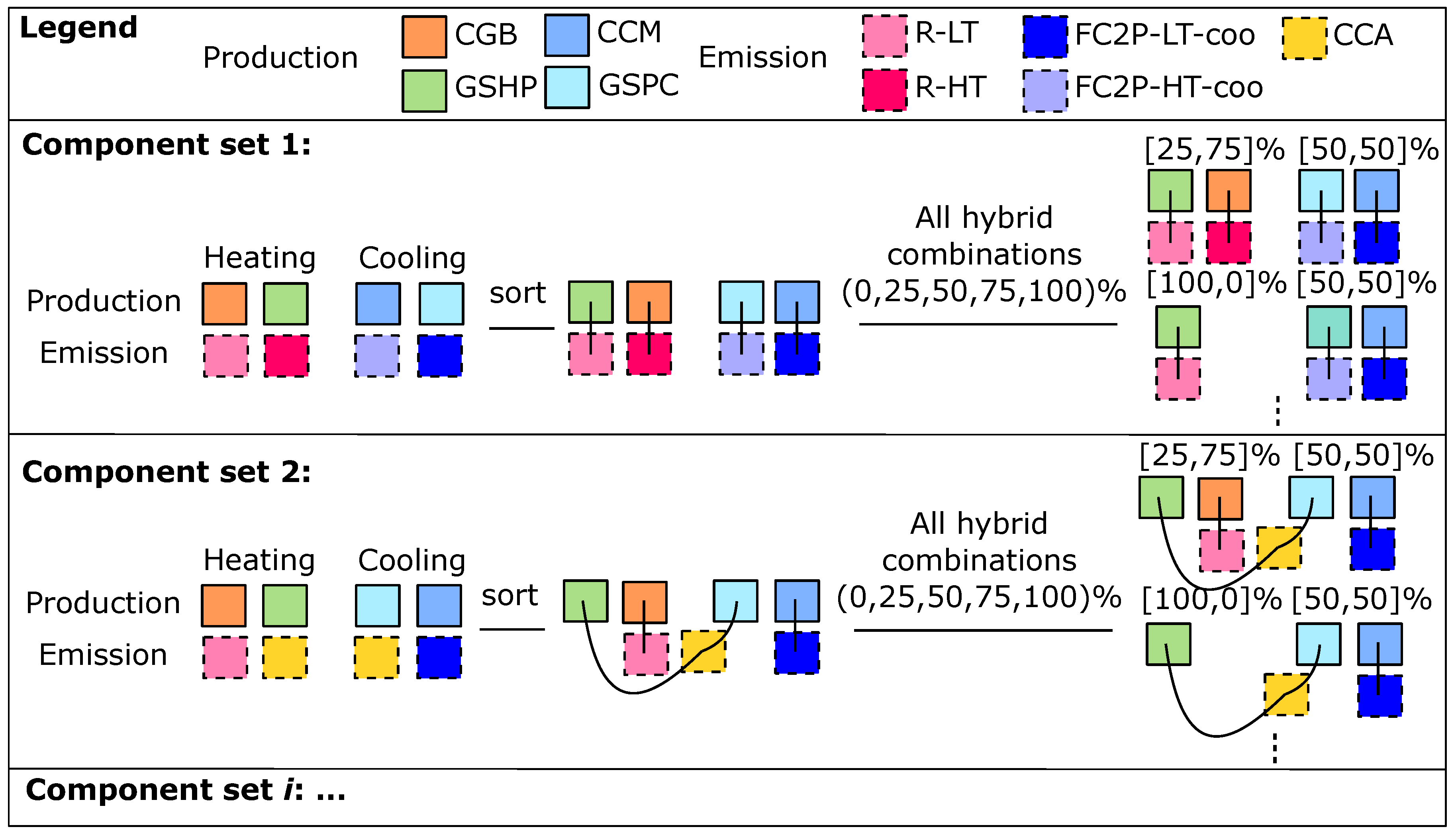
The second step is to generate all possible HVAC scenarios composed of the devices present in the database, which can deliver the energy and thermal powers of the given LDC using the HVAC components of the database. In order to limit the number of possible scenarios, a scenario can contain a maximum of two heat and two cold production systems, each coupled to its own emission system. Note that reversible components count for two: one for heating, one for cooling. Figure 2 illustrates how the different scenarios are generated. Firstly, a set of production and emission systems is taken from the available components of the database. Secondly, the production systems are sorted by decreasing efficiency and the heat (cold) emission system with the lowest (highest) supply temperature is coupled to the most efficient heat (cold) production system. The maximum heating (cooling) power present in the LDC can now be divided between the two heat (cold) systems according to predefined hybrid fractions (currently set as [0, 25, 50, 75, 100]%). Note that both the heating and the cooling hybrid fractions can vary independently, that coupled production and emission systems are sized together, and that, when a 0% hybrid fraction is allocated, this means that the component is not installed. When a reversible system is installed, it will be sized by the maximum of its heating and cooling powers, taking its cooling to heating power conversion factor (see Table 3) into account. This is necessary as, for example, the cooling power of a high temperature 4 pipes fan coil unit (FC4P-HT) at its nominal conditions is only 60% of its heating power due to the smaller temperature difference between the air of the zone and the fan coil supply water for cooling than for heating.
While most of the components are sized according to their nominal power, CCA and Floor Heating (FH) are sized to a realistic fixed 80% of the building floor surface area and the ground heat exchanger (i.e., the borefield) is automatically designed according to the standard ISSO73 [32]. Standard ISSO73 returns the number of boreholes and their depth necessary to deliver a given maximum thermal power and a given amount of yearly energy and it takes into account the regeneration level, the ground and grout characteristics, the borefield configuration, the borehole type, the maximum borehole depth, and the minimum allowed ground temperature (). The standard was originally developed to size heating dominated borefields based on the results returned by the Energy Earth Design (EED) software [33] with an accuracy of ±10%. In this work, the work flow proposed by the standard has been translated in the Python tool to automatically size the borefield and the method is extended as follows to allow cooling dominated cases. When the borefield is heating dominated, its sizing depends on the temperature difference between the initial ground temperature () and . In Belgium, this temperature difference is typically around 10 C as is typically around 10 C and is here chosen equal to 0 C to avoid freezing of the ground. When the borefield is cooling dominated, the borefield is sized such that the ground temperature does not exceed a maximum value (), which is chosen in this work to be 17 C, to ensure that passive cooling with the ground can always be used. The same work flow can then be applied to size cooling dominated borefields by simply using the cooling energy and power instead of the heating ones and by choosing so that , which means C for the mentioned assumptions.
Finally, the original energy of the LDC, which corresponds to the building energy needs for space heating and cooling, is corrected to include the emission system efficiency as specified by the standard NBN EN15316-2-1:2007 [34] (see Section 5 and Table 3).
Step 3: Compute energy use, costs and emissions
Once the type and the size of each HVAC component of a scenario are defined, the energy from the LDC can be allocated to the different production components such that the most efficient component delivers the base load. Notice that Figure 1 shows only one LDC while actually two LDCs are needed: one for heating, one for cooling. The scenario present cost (PC) can now be computed as:
with the initial investment cost calculated as the sum of the different component cost functions (see Table 1), N the number of years during which the system will be used (in this work, 20 years is assumed), , , and the energy, maintenance, and replacement costs computed using the efficiencies, maintenance percentages, and life expectancies of Table 1, Table 2 and Table 3 and a given electricity and gas price of 0.1466 and 0.0534 €/kWh [35,36], and the remaining value of the system after N years. Note that the investment cost of the components and the energy prices are assumed to stay constant over the years and no inflation is considered. This assumptions are chosen due to the too high uncertainty on those factors and in order to keep the computations more transparent. However, the different costs are discounted with discount factor with j the number of years counted from the investment time and i the discount rate. An interest rate of 4% is used in this work. is further calculated linearly with the number of years the device can still be used except for radiators, CCA and the ground heat exchanger (GHEX-V) for which is zero as they cannot be easily dismantled and re-used.
Besides the PC, the total CO emissions caused by the energy use of the building are computed using the primary energy conversion factor of 0.056 kg/MJ for gas and 0.179 kg/MJ for electricity [10].
Step 4: Choose the most appropriate HVAC system
The final step compares the PC and the total CO emission of each scenario over a realistic 20 years lifetime of the building such that the design engineer can make the most appropriate choice.
4. Assumptions and Limitations
The main assumption/limitation of the presented methodology is that the LDC of the building is assumed given and therefore no dynamic simulations have been carried out. In the future, the method should include an LDC generator. The powers and energy of the LDC furthermore depend on the chosen HVAC scenario, which is taken into account by the emission efficiencies from NBN EN 15316-2-1:2007 [34]. However, the accuracy of such efficiencies should be investigated by dynamic simulations. Finally, as no dynamic simulations are carried out, comfort cannot be explicitly checked. The method assumes that, if the HVAC system can provide the thermal load defined by the LDC, comfort will be guaranteed and it is up to the designer to choose the most comfortable HVAC system, while taking into account the energy use, costs and emissions returned by the method.
The following assumptions are also made:
- While different efficiencies for different supply temperatures are used, the nominal power of production devices does not depend on their supply temperature. This might cause an over or underestimation of the device investment cost when it is used in different nominal conditions.
- For geothermal systems, only the most common vertical ground heat exchangers (GHEX-V) are considered. Furthermore, it is assumed that Ground Source Heat Pumps (GSHP) are not reversible and that cooling can only be done passively using a GSPC. This assumption might cause an overestimation of the investment cost of GSHP systems.
- If CCA or FH is installed, it is assumed that it will be installed for the whole building and cover a fixed 80% of the building floor surface area.
- So far, the ventilation system and the building climate controller are not included in the HVAC design optimization while they may have a significant impact on the investment cost, energy use and achieved comfort. In addition, the number of considered HVAC components is limited (see Table 1).
- No inflation is taken into account due to its large uncertainty, but all costs are discounted as described in Section 3.
5. Components Information
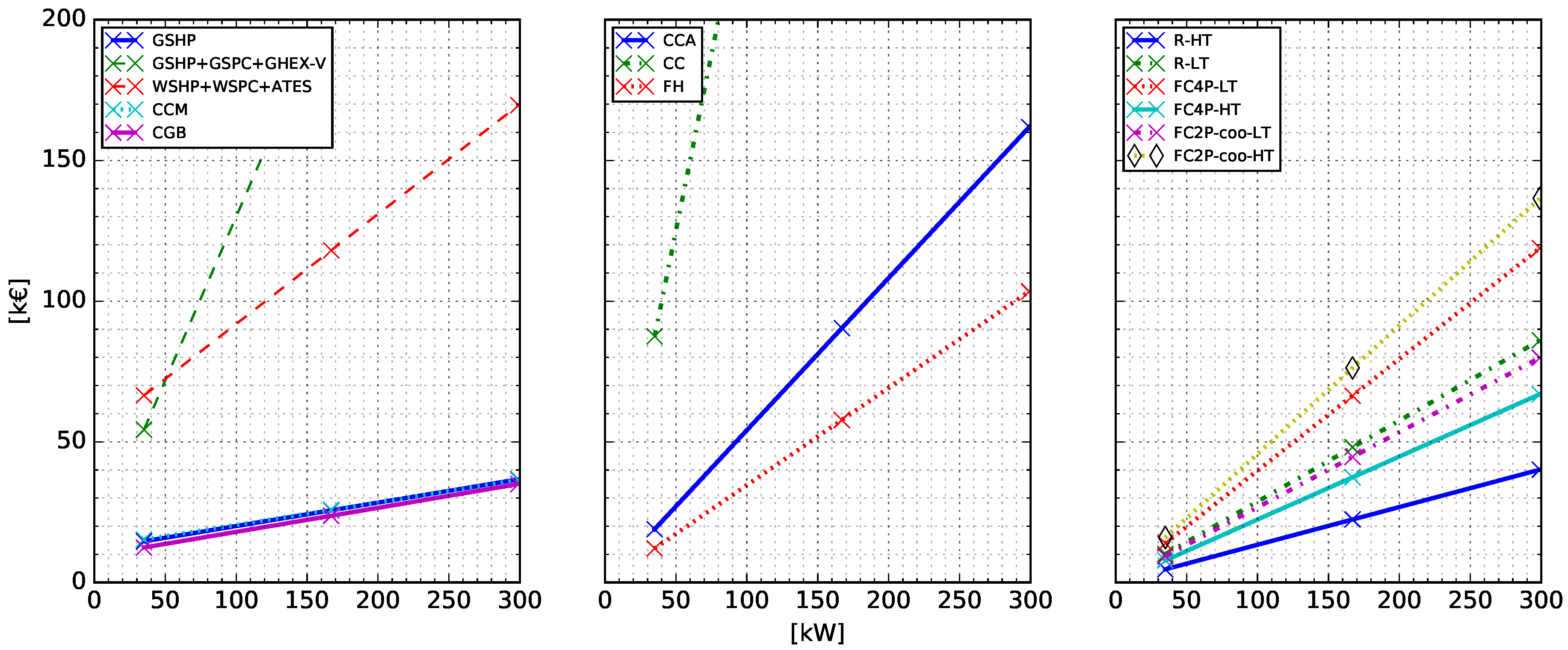
As described in Section 3, the first step to optimize the HVAC system is to gather the necessary information about its components. The nomenclature, the cost function, the maintenance cost, and the life expectancy of each considered HVAC component are listed in Table 1 and the cost functions are also represented in Figure 3. The cost functions are derived from the (installed) cost data of 18 recently built buildings from two different Belgian engineering offices. The maintenance costs, expressed as a percentage of the investment cost, and the life expectancies are retrieved from the standard NBN EN 15459 [37]. The database can easily be extended with new components and the required parameters are known.
Table 2 contains the assumed energy conversion efficiencies of the different heat and cold production components for different supply temperatures, based on the average of values found in technical sheets of different manufacturers and in the Annex 48 report [39]. When the efficiency is not given, it means that the component cannot supply water at that particular temperature. For the emission components, Table 3 indicates their nominal conditions for heating and cooling, the ratio between their cooling and their heating power and their efficiency. The emission system effiencies are taken from NBN EN15316-2-1:2007, and they represent the system additional heat losses. These heat losses are due to the non-uniform internal temperature distribution in the conditioned zones (caused by stratification, heat emitters along outside wall/window, differences between air temperature and mean radiant temperature), the non-ideality of the operative temperature control (causing temperature variations and drift) and the extra heat losses of heat emitters embedded in the building structure towards the outside.
6. Results
In this section, two types of scenarios are considered: (i) the so-called minimum scenarios (M-Sce) that are composed of one single production system for heating and one for cooling, each coupled to its own emission system (see Section 6.1), and (ii) so-called hybrid scenarios (H-Sce) composed of two heating and two cooling systems (see Section 6.2). For both M-Sce and H-Sce, their PC over 20 years and their yearly CO emissions are compared for different parameter values. In the case of M-Sce, the PC only depends on the maximum heating () and cooling () powers, and on the total yearly amount of heating () and cooling energy () delivered to the building. Additionally, the building floor surface area () and the ground thermal conductivity () can influence the scenarios PC if it uses CCA and a GSHP. In the case of H-Sce, the shape of the LDC is also important as it defines the ratio between the energy covered by the base load system and the energy covered by the peak load system.
In order to limit the degrees of freedom, the parametric space is represented in this work by five parameters: , FLHh, , , and . FLHh is the number of full load hours that the heat production system runs per year. Multiplying FLHh with gives thus . The parameter is defined as and its value indicates whether the building is heating (%) or cooling dominated (%) or in thermal balance (%). Note that a GEOTABS-scenario (GEOTABS-M-Sce) (i.e., a scenario only composed of a GSHP, a GSPC and CCA) with % does not have a borefield with a balanced heating and cooling load as a fraction of the heat comes from the electricity use of the GSHP and not from the ground. In this work, is varied by changing the ratio while the number of full load hours of the cold production device () is always kept equal to FLHh. The influence of is represented by the maximum specific power per unit floor area: . Finally, is used as an indicator of the ground suitability for GSHP systems. The values of these five parameters are taken from realistic ranges for large Belgian buildings (see Table 4). The range for is further chosen such that the cost functions of the production components are always evaluated within their validity ranges, even when hybrid systems are installed (see Section 6.2), and is kept equal to 27 for M-Sce to ensure that the maximum heating and cooling powers can be provided by CCA without auxiliary emission systems, even for the maximum value of %.
For the reader’s convenience, the meaning of the different symbols and abbreviations used thoroughout this chapter are summarized in Table 1, Table 4 and Table 5. Figures 5–10 furthermore use the following convention for the legend entries: each keyword separated by ’/’ represents an HVAC component installed in the scenario, and the number following the keyword indicates its nominal power as a fraction of for heating devices and for cooling devices. For example, for a LDC with kW, GSHP0.75/CGB0.25/GSPC1/R-HT0.25/CCA means that the scenario is composed of a GSHP of 112.5 kW, a CGB of 37.5 kW, R-HT with a total power of 37.5 kW and CCA (for which no fraction is given as CCA is assumed to always cover the whole building floor surface area).
6.1. Results for Single Production/Single Emission Scenarios
In this section, scenarios (M-Sce) composed of a single heat and single cold production system, each coupled to its own emission system, are considered.
Figure 4 plots the PC of each M-Sce for the different parameter values of Table 4. Each row assumes a different FLHh and , each column a different while the x-axes specify , and each line represents a different M-Sce. The lines representing GEOTABS-M-Sce are plotted in green with square markers and the lines referring to the most conventional scenario type (Conv-M-Sce) (composed of a CGB, a CCM and FC4P-HT) are plotted in red with diamond markers. Finally, the background of the graphs is set in blue if GEOTABS-M-Sce extract more heat from the ground than they inject (i.e., the borefield is heating dominated) and in orange otherwise.
From Figure 4, it appears that, in general, Conv-M-Sce are the most cost efficient M-Sce that can be installed. When only a low cooling load is required (%), Conv-M-Sce are a factor 1.0 to 1.7 cheaper than GEOTABS-M-Sce and for cooling dominated buildings (%), the factor varies between 1.2 to 1.8. Only the cases when the cooling and heating loads of the borefield are in balance (i.e., % for a COP = 5.6) and when the building uses a minimum of 1750 FLHs, GEOTABS-M-Sce are financially advantageous (up to a factor 1.1 for the highest and FLH). Interestingly, the lines representing the different M-Sce do not cross each other for different which means that the cost optimal M-Sce (M-Sce*) for the investigated parameter values do not depend on . The cooling dominated columns of Figure 4 (%) further indicate that other M-Sce than Conv-M-Sce can be cost optimal. This is illustrated in Figure 5.
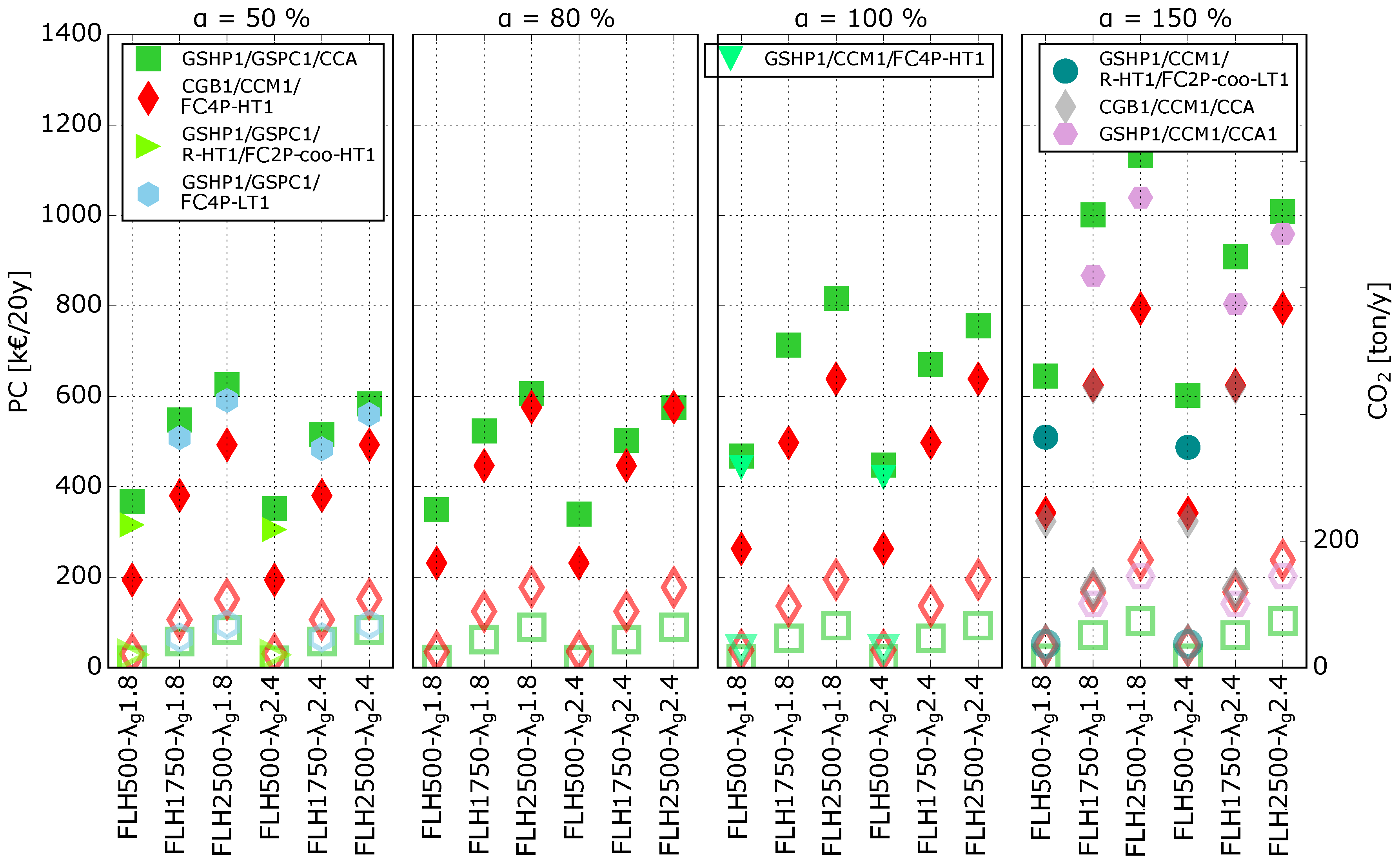
Figure 5 contains the same information as Figure 4 evaluated at kW, but the CO emissions are added to the figure. The left y-axis represents the PC (filled markers) of the M-Sce (in €/20y) and the right y-axis returns the CO emissions (unfilled markers) in ton/1y, the x-axes indicate the number of FLHh and , and each subplot corresponds to a different value. For each condition, the GEOTABS-M-Sce and the Conv-M-Sce are plotted with green square markers and red diamond markers, respectively. Additionally, M-Sce* and the cost optimal geothermal scenario (Geo-Sce*) are also included if they differ from GEOTABS-M-Sce and Conv-M-Sce. Finally, the CO emissions of each plotted scenario are represented by the same (but unfilled) marker, and their value is to be read on the right axis.
Figure 5 shows that, when a large amount of cooling is required ( is high), GEOTABS-M-Sce are systematically (much) more expensive than Conv-M-Sce despite the fact that cooling with GEOTABS-M-Sce is more energy efficient (EER = 20) than with Conv-M-Sce (EER = 3.9). This is due to the fact that the borefields of GEOTABS-M-Sce with % are sized according to the cooling load, which leads to larger, thus (much) more expensive, borefields. By sizing the borefield only for the heating load and covering the cooling load with a CCM (GSHP1/CCM1/CCA1 markers in Figure 5), the scenario price could be decreased by a factor up to 1.3. The cost of the Geo-Sce can further be reduced by allowing a hybrid design such that the borefield would deliver only a fraction of the cooling load (see Section 6.2). Similarly, the FC4P-HT are becoming very expensive when they are used for unbalanced loads. The scenarios GSHP1/CCM1/CCA1 and those combining GSHP, GSHPC, R-HT, and FC2P-coo-HT can therefore become cheaper as the use of the expensive FC4P-HT can then be avoided. In the case of a thermally balanced borefield (%), the GEOTABS-M-Sce become very advantageous and their PC drops below those of Conv-M-Sce for buildings using at least 1750 FLH while they emit 58% less CO2. Finally, the use of R-LT and FC4P-LT instead of their high temperature equivalent appears not to be advantageous to be coupled to the condensing gas boiler and cooling machine as their additional investment costs are not compensated by the realized energy savings.
While GEOTABS-M-Sce are in general more expensive than Conv-M-Sce, Figure 5 also shows that GEOTABS-M-Sce emit between 64% (for %) and 55% (for %) less CO than Conv-M-Sce.
6.2. Results for Hybrid Scenarios
This section is similar to Section 6.1, but hybrid scenarios (H-Sce) are now allowed with a maximum of two heat and two cold production systems, each coupled to its own emission system (see Section 3). H-Sce depend on the same parameters as M-Sce (see Table 4), but the shape of the LDC now also influences their PC and CO emissions. Therefore, two types of LDC are used, i.e., triangular and logarithmic, as represented in Figure 6. Furthermore, two different values of are considered in this section (27 and 70 W/m, see Table 4), as the CCA can now be complemented with a second emission system both for heating and cooling.
The following figures representing the PCs and CO emissions of H-Sce for the different boundary conditions contain the following information. Firstly, as H-Sce can become a M-Sce if only 0% and 100% hybrid factions are used, green squares and red diamonds still represent GEOTABS-M-Sce and Conv-M-Sce, respectively. Note, however, that, when W/m, H-Sce will not contain any GEOTABS-M-Sce as the CCA cannot provide the thermal power without an auxiliary emission system. Secondly, the cost optimal geothermal scenario (Geo-Sce*) is also plotted in each figure. Finally, if the overall cost optimal H-Sce (H-Sce*) does not coincide with an already plotted scenario, H-Sce* is added to the figure.
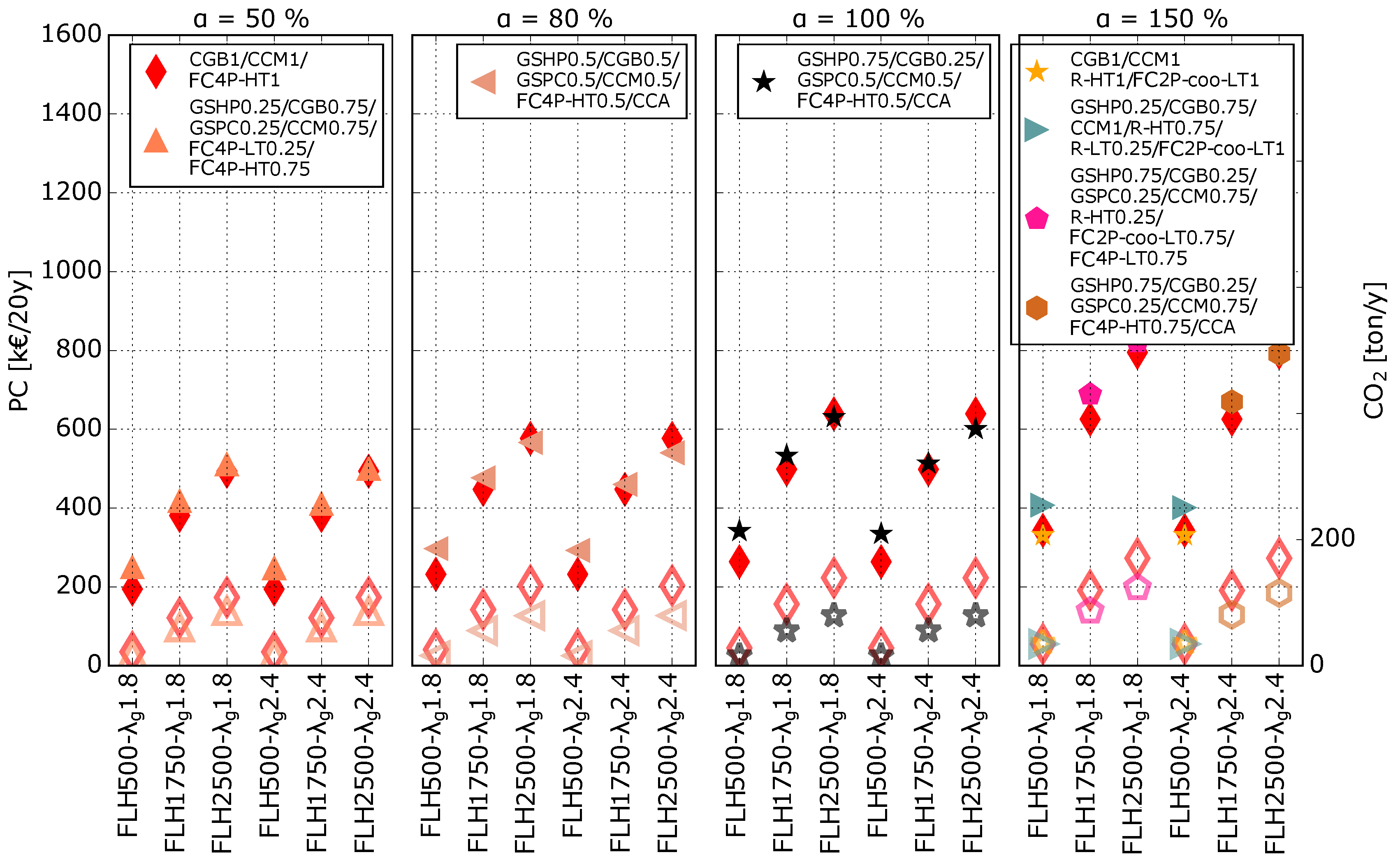
6.2.1. Triangular LDCs
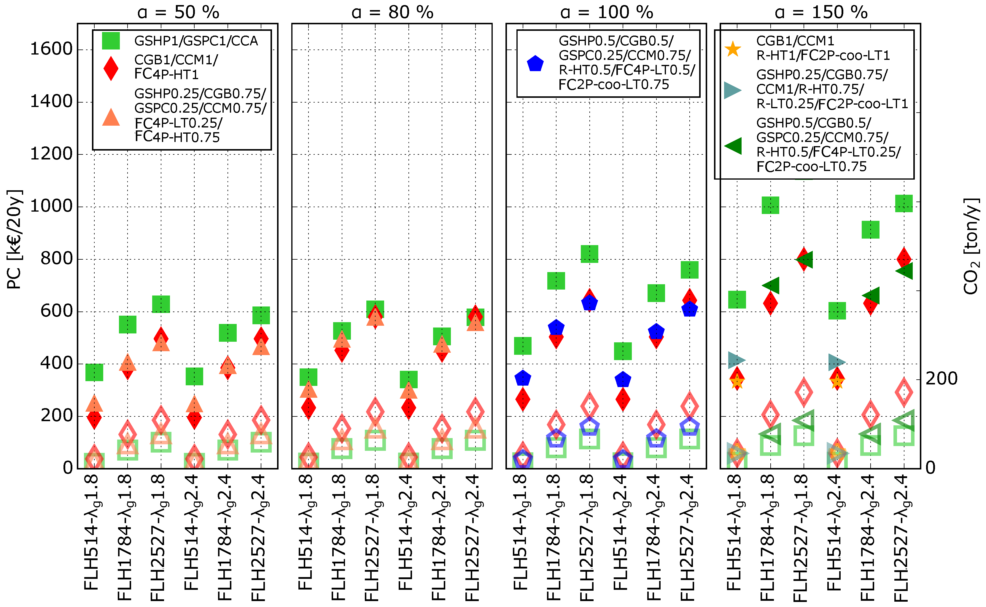
The shapes of the triangular LDCs are chosen such that they correspond to the , FLHh, and values of Table 4. Figure 7 and Figure 8 assume a of 27 W/m and 70 W/m, respectively, resulting in different optimal scenarios as the CCA (if installed) is a factor 2.6 cheaper for the latter (CCA are assumed to cover a fixed 80% of the building floor surface area), but it needs to be complemented with an auxiliary emission system to provide enough thermal power.
In the case when W/m, the results for Conv-M-Sce and GEOTABS-M-Sce are the same as in Section 6.1. Figure 7 shows that, for heating dominated buildings, Geo-Sce* are generally composed of a combination of a GSHP (25%) and a GSPC (25%) coupled to FC4P-LT and of a CGB (75%) and a CCM (75%) coupled to FC4P-HT. Here, the Geo-Sce* remain a factor 1.03 to 1.28 more expensive than the Conv-M-Sce but emit 20% less CO than Conv-M-Sce. For cooling dominated cases, installing a GSPC covering only a fraction of the required cooling power (25 to 50%) significantly reduces the PC cost differences between Conv-M-Sce and Geo-Sce* to such an extent that Geo-Sce* become the H-Sce* for buildings with large energy loads (2500 FLH). Furthermore, Geo-Sce* systematically reduce the CO emission by more than 50% compared to Conv-M-Sce.
As illustrated by Figure 8, in the case when W/m, Geo-Sce coupled to CCA and FC4P-HT are the optimal scenarios H-Sce* when and have similar cost as Conv-M-Sce for %. For example, Geo-Sce* can be up to 1.1 cheaper than Conv-M-Sce when % and up to 1.2 when % while Geo-Sce* save in both situations around 50% of the CO emissions.
6.2.2. Logarithmic LDCs
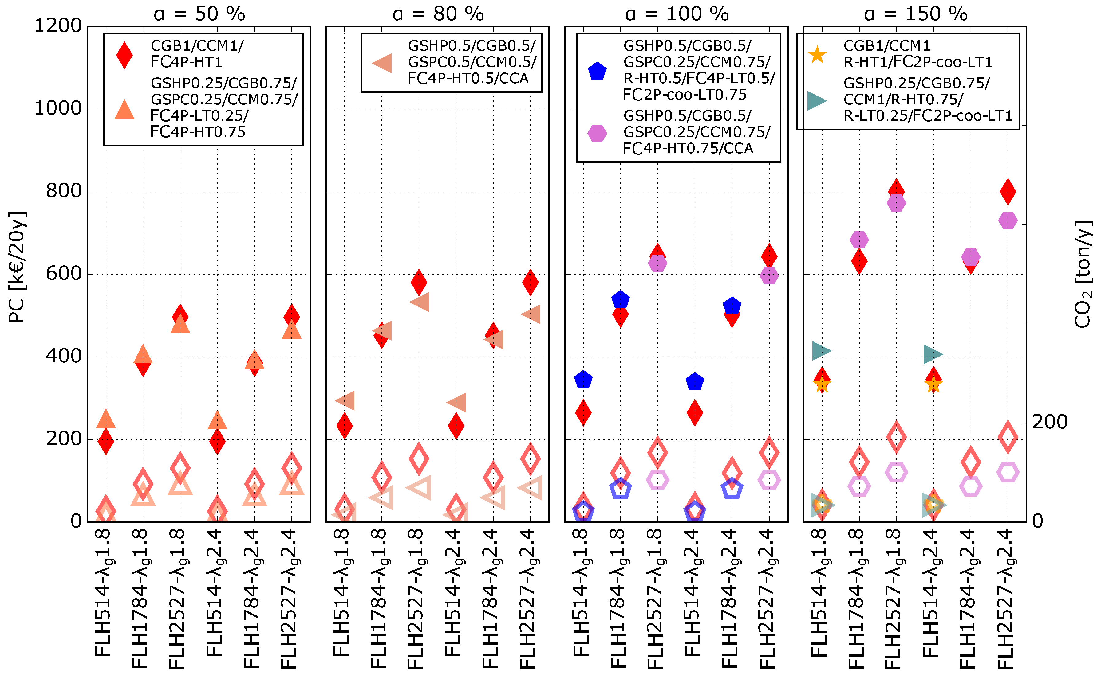
LDCs have rather an (inverted) logarithmic shape than a triangular shape, and this paragraph therefore investigates the cost optimality of HVAC scenarios for LDCs described by with x the number of hours and the heating power. The parameter influences the steepness of the curve and and are calculated such that the different LDCs correspond to the parameter values of Table 4, and such that the LDCs tail is cut at (see Figure 6). The results are again analysed for and 70 W/m(see Figure 9 and Figure 10).
The results for logarithmic LDCs are very similar to those for the triangular LDCs. However, where the Geo-Sce* from the triangular LDCs would most of the time size its GSHP to 75% and its GSPC to 50 or 25%, the Geo-Sce* from the logarithmic LDCs would rather size them to 50% and 25%, respectively. This is a logical result as the number of FLH for the higher thermal powers decreases faster for logarithmic LDCs than for triangular ones. This also results in a lower PC for the Geo-Sce with logarithmic LDC while Conv-M-Sce and GEOTABS-M-Sce remain the same. For example, the Geo-Sce* is 1.25 times cheaper than Conv-M-Sce when FLH=2527 h, W/(m K) and W/m and still saves 50% of the CO emissions.
7. Conclusions
This chapter presents a tool developed in Python to automatically compute the present cost (PC) and CO emissions of all possible HVAC designs of a given building composed of the devices contained in the database. The tool was used to investigate when HVAC systems using a vertical ground heat exchanger (GHEX-V) become economically interesting and to compare their CO emissions to those of a conventional HVAC system which uses a condensing gas boiler, a compression cooling machine and reversible high temperature four pipes fan coil units.
It was found that pure GEOTABS systems (i.e., an HVAC system composed of a GSHP system coupled to CCA) for buildings with a thermal power between 150 and 250 kW are generally 1.0 to 1.8 times more expensive than a conventional HVAC system when the GHEX-V is not in thermal balance but that pure GEOTABS systems have the lowest PC of all possible scenarios when ground thermal balance is reached and the building uses its GSHP system for at least 1750 full load hours (FLH) per year. For all cases, pure GEOTABS systems save more than 50% of CO emissions compared to a conventional one.
It was further shown that, instead of installing pure GEOTABS systems, combining a GSHP system with TABS to cover the base load of the building and a condensing gas boiler and a cooling machine with fan coil units and/or radiators, results in hybrid GEOTABS systems with a PC that is lower than or similar to the PC of a conventional system, while still between 20% to more than 50% of CO emissions are saved. Hybrid GEOTABS concepts can thus be very advantageous both economically and for the environment.
Acknowledgments
The authors gratefully acknowledge the financial support by the IWT and WTCB in the frame of the IWT-VIS Traject SMART GEOTHERM focusing on integration of thermal energy storage and thermal inertia in geothermal concepts for smart heating and cooling of (medium) large buildings. The authors also acknowledge the funding of their research work by the EU within the H2020-EE-2016-RIA-IA programme for the project ‘Model Predictive Control and Innovative System Integration of GEOTABS;-) in Hybrid Low Grade Thermal Energy Systems - Hybrid MPC GEOTABS’ (grant number 723649 - MPC-; GT). The authors would further like to thank Boydens Engineering (Zedelgem, Belgium) and Ingenium N.V. (Brugge, Belgium) for sharing their cost data.
Author Contributions
Damien Picard designed the methodology, performed the calculations, analyzed the results and wrote the paper. Lieve Helsen provided guidance during the research work and reviewed the manuscript.
Conflicts of Interest
The authors declare no conflicts of interest.
Abbreviations
The following abbreviations are used in this manuscript:
| HVAC | Heating Ventilation and Air Conditioning |
| PC | Present Cost |
| MILP | Mixed Integer Linear Programming |
| LDC | Load Duration Curve |
| GSPC | Ground Source Passive Cooling |
| GSHP | Ground Source Heat Pump |
| GHEX-V | Vertical Ground Heat Exchanger |
| CCA | Concrete Core Activation |
| FH | Floor Heating |
| TABS | Thermally Activated Building Structure |
| FC4P | Fan Coil Unit 4 pipes |
| HT | High Temperature |
| LT | Low Temperature |
| CGB | Condensing Gas Boiler |
| CCM | Compression Cooling Machine |
| R | Radiator |
| TS | Technical Sheet |
References
- Perez-Lombard, L.; Ortiz, J.; Pout, C. A review on buildings energy consumption information. Energy Build. 2008, 40, 394–398. [Google Scholar] [CrossRef]
- European Parliament. Directive 2010/31/EU of the European Parliament and of the Council of 19 May 2010 on the energy performance of buildings (recast). Off. J. Eur. Union 2010, 18, 2010. [Google Scholar]
- Ellis, M.; Mathews, E. Needs and trends in building and HVAC system design tools. Build. Environ. 2002, 37, 461–470. [Google Scholar] [CrossRef]
- Nguyen, A.T.; Reiter, S.; Rigo, P. A review on simulation-based optimization methods applied to building performance analysis. Appl. Energy 2014, 113, 1043–1058. [Google Scholar] [CrossRef]
- Ooka, R.; Komamura, K. Optimal design method for building energy systems using genetic algorithms. Build. Environ. 2009, 44, 1538–1544. [Google Scholar] [CrossRef]
- Seo, J.; Ooka, R.; Kim, J.T.; Nam, Y. Optimization of the HVAC system design to minimize primary energy demand. Energy Build. 2014, 76, 102–108. [Google Scholar] [CrossRef]
- Ashouri, A.; Fux, S.; Benz, M.; Guzzella, L. Optimal design and operation of building services using mixed-integer linear programming techniques. Energy 2013, 59, 365–376. [Google Scholar] [CrossRef]
- Patteeuw, D.; Helsen, L. Combined design and control optimization of residential heating systems in a smart-grid context. Energy Build. 2016, 133, 640–657. [Google Scholar] [CrossRef]
- Evins, R. Multi-level optimization of building design, energy system sizing and operation. Energy 2015, 90, 1775–1789. [Google Scholar] [CrossRef]
- Vergaert, V.; Parys, W.; Marten, D. Studie Naar Kostenoptimale Niveaus van de Minimumeisen Inzake Energieprestaties van Niet-Residentiële Gebouwen; Technical Report for Vlaams Energieagentschap: Geel, Belgium, 2015. [Google Scholar]
- Henze, G.P.; Felsmann, C.; Kalz, D.E.; Herkel, S. Primary energy and comfort performance of ventilation assisted thermo-active building systems in continental climates. Energy Build. 2008, 40, 99–111. [Google Scholar] [CrossRef]
- Kalz, D.E. Heating and Cooling Concepts Employing Environmental Energy and Thermo-Active Building Systems, System Analysis and Optimization. Ph.D. Thesis, University of Karlsruhe, Stuttgart, Germany, 2011. [Google Scholar]
- Bockelman, F.; Plesser, S.; Soldaty, H. Advanced System Design and Operation of GEOTABS Buildings: Design and Operation of GEOTABS Systems; Rehva: Brussels, Belgium, 2013. [Google Scholar]
- Sourbron, M.; Helsen, L. Thermally activated building systems in office buildings: Impact of control strategy on energy performance and thermal comfort. In Proceedings of the International Conference on System Simulation in Buildings, Liege, Belgium, 13–15 December 2010. [Google Scholar]
- Sourbron, M.; De Herdt, R.; Van Reet, T.; Van Passel, W.; Baelmans, M.; Helsen, L. Efficiently produced heat and cold is squandered by inappropriate control strategies: A case study. Energy Build. 2009, 41, 1091–1098. [Google Scholar] [CrossRef]
- Tian, Z.; Love, J.A. Energy performance optimization of radiant slab cooling using building simulation and field measurements. Energy Build. 2009, 41, 320–330. [Google Scholar] [CrossRef]
- Treiber, M. Nutzenübergabe Thermoaktiver Decken. Ph.D. Thesis, University of Stuttgart, Stuttgart, Germany, 2007. [Google Scholar]
- Sourbron, M.; Helsen, L. Slow thermally activated building system and fast air handling unit join forces through the use of model based predictive control. In Proceedings of the CLIMA 2013 Congress, Prague, Czech Republic, 16–19 June 2013; pp. 1–10. [Google Scholar]
- Sourbron, M. Dynamic Thermal Behaviour of Buildings with Concrete Core Activation. Ph.D. Thesis, Department of Mechanical Engineering, KU Leuven, Leuven, Belgium, 2013. [Google Scholar]
- Olesen, B.W.; Liedelt, D. Cooling and heating of buildings by activating their thermal mass with embedded hydronic pipe systems. In Proceedings of the CIBSE Conference, Dublin, Ireland, 2000. [Google Scholar]
- Tödtli, J.; Güntensperger, W.; Gwerder, M.; Haas, A.; Lehmann, B.; Renggli, F. Control of concrete-core conditioning systems. In Proceedings of the 8th REHVA World Congress, Lausanne, Switzerland, 9–12 October 2005. [Google Scholar]
- Tödtli, J.; Gwerder, M.; Lehmann, B.; Renggli, F.; Dorer, V. TABS-Control: Steuerung und Regelung von Thermoaktiven Bauteilsystemen; Faktor Verlag: Zurich, Switzerland, 2009; Volume 86. [Google Scholar]
- Olesen, B.W. Radiant heating and cooling by embedded water-based systems. In Proceedings of the Congreso Climaplus 2011, Madrid, Spain, 1–2 March 2011. [Google Scholar]
- Picard, D. Modeling, Optimal Control and HVAC Design of Large Buildings Using Ground Source Heat Pump Systems. Ph.D. Thesis, Department of Mechanical Engineering, KU Leuven, Leuven, Belgium, 2017. [Google Scholar]
- Oldewurtel, F.; Parisio, A.; Jones, C.N.; Gyalistras, D.; Gwerder, M.; Stauch, V.; Lehmann, B.; Morari, M. Use of model predictive control and weather forecasts for energy efficient building climate control. Energy Build. 2012, 45, 15–27. [Google Scholar] [CrossRef]
- Gyalistras, D.; Gwerder, M. Use of Weather and Occupancy Forecasts For Optimal Building Climate Control (OptiControl), Two Years Progress Report; Technical Report; Terrestrial Systems Ecology ETH Zurich: Zurich, Switzerland, 2009. [Google Scholar]
- Sturzenegger, D.; Gyalistras, D.; Gwerder, M.; Sagerschnig, C.; Morari, M.; Smith, R.S. Model Predictive Control of a Swiss office building. In Proceedings of the 11th REHVA World Congress Clima, Prague, Czech Republic, 16–19 June 2013. [Google Scholar]
- Váňa, Z.; Cigler, J.; Širokỳ, J.; Žáčeková, E.; Ferkl, L. Model-based energy efficient control applied to an office building. J. Process Control 2014, 24, 790–797. [Google Scholar] [CrossRef]
- Prívara, S.; Široký, J.; Ferkl, L.; Cigler, J. Model predictive control of a building heating system: The first experience. Energy Build. 2011, 43, 564–572. [Google Scholar] [CrossRef]
- Michailidis, I.T.; Baldi, S.; Pichler, M.F.; Kosmatopoulos, E.B.; Santiago, J.R. Proactive control for solar energy exploitation: A german high-inertia building case study. Appl. Energy 2015, 155, 409–420. [Google Scholar] [CrossRef]
- Baldi, S.; Michailidis, I.; Ravanis, C.; Kosmatopoulos, E.B. Model-based and model-free “plug-and-play” building energy efficient control. Appl. Energy 2015, 154, 829–841. [Google Scholar] [CrossRef]
- ISSO. ISSO73: Ontwerp en Uitvoering van Verticale Bodemwarmtewisselaar; Kennisinstituut Bouw-en Installatietechniek: Rotterdam, The Netherlands, 2005. [Google Scholar]
- Hellström, G.; Sanner, B. Earth Energy Designer, User Manual, Version 2.0; Department of Mathematical Physics, Lund University: Lund, Sweden, 2000. [Google Scholar]
- Technical Committee CEN/TC 228. NBN EN 15316-2-1:2007: Heating Systems in Buildings—Method for Calculation of System Energy Requirements and System Efficiencies—Part 2-1: Space Heating Emission Systems; European Committee for Standardization: Brussels, Belgium, 2007. [Google Scholar]
- Eurostat. Electricity Prices Components for Industrial Consumers—Annual Data (From 2007 Onwards). Available online: http://appsso.eurostat.ec.europa.eu/nui/submitViewTableAction.do (accessed on 8 March 2017).
- Eurostat. Gas Prices for Industrial Consumers—Bi-Annual Data (From 2007 Onwards). Available online: http://ec.europa.eu/eurostat/web/energy/data/database (accessed 21 February 2017).
- Technical Committee CEN/TC 156. NBN EN 15459:2007: Energy Performance of Buildings—Economic Evaluation Procedure for Energy Systems in Buildings; Bureau voor Normalisatie: Brussels, Belgium, 2007. [Google Scholar]
- Verheyden. Boringen Verheyden Bvba. 2017. Available online: http://www.boringenverheyden.be (accessed on 14 August 2017).
- Bertagnolio, S.; Stabat, P.; Caciolo, M.; Corgier, D. IEA ECBCS Annex 48 Reversible Air-Conditioning: Review of Heat Recovery and Heat Pumping Solutions; International Energy Agency: Liege, Belgium, 2011. [Google Scholar]
- Riello. Systèmes à Condensation: Riello Tau N, Riello Tau Premix. 2017. Available online: http://sos-express.be/wp-content/uploads/2015/11/Riello-RIELLO-TAU-PREMIX.pdf (accessed on 16 February 2017).
- AlphaInnoTec. Brine/Water Warmtepompen, Warmtecentrale Brine—Instalatlatie- en Gebruikshandleiding. 2017. Available online: http://www.nathan.be/uploads/public/83053100bNL_BA_WZS_1.pdf (accessed on 16 February 2017).
- Carrier. Water-Sourced Liquid Chillers/Heat Pumps with or without Integrated Hydronic Module. 61 WG/30WG. 2017. Available online: http://carrierab.se/media/49347/16121_psd_02_2012_61wg_30wg_lr.pdf (accessed on 16 February 2017).
- Viessmann. Installation and Service Instruction, VITOCAL 300-G. 2017. Available online: http://www.viessmann.com/vires/product_documents/5600161VSA00002_1.PDF (accessed on 16 February 2017).
Figure 1.
Schematic representation of the optimal Heating, Ventilation and Air-Conditioning (HVAC) design methodology split in four consecutive steps. The generation of load duration curves (LDC) based on a limited set of building parameters is not yet implemented and is therefore represented as a dotted grey arrow.

Figure 2.
Illustration of how different HVAC scenarios composed of two heat and two cold production devices, each coupled to its own emission component.
Figure 2.
Illustration of how different HVAC scenarios composed of two heat and two cold production devices, each coupled to its own emission component.

Figure 3.
Cost function of each component included in the database. 30 W/m for the borefield and 40 W/m (heating) for Concrete Core Activation (CCA) are assumed to convert the cost function variable to kW. All powers correspond to the nominal heating power of the device, except for FC2P-coo-LT and FC2P-coo-HT for which the nominal cooling power is used instead. The meaning of the legend entries can be found in Table 1.

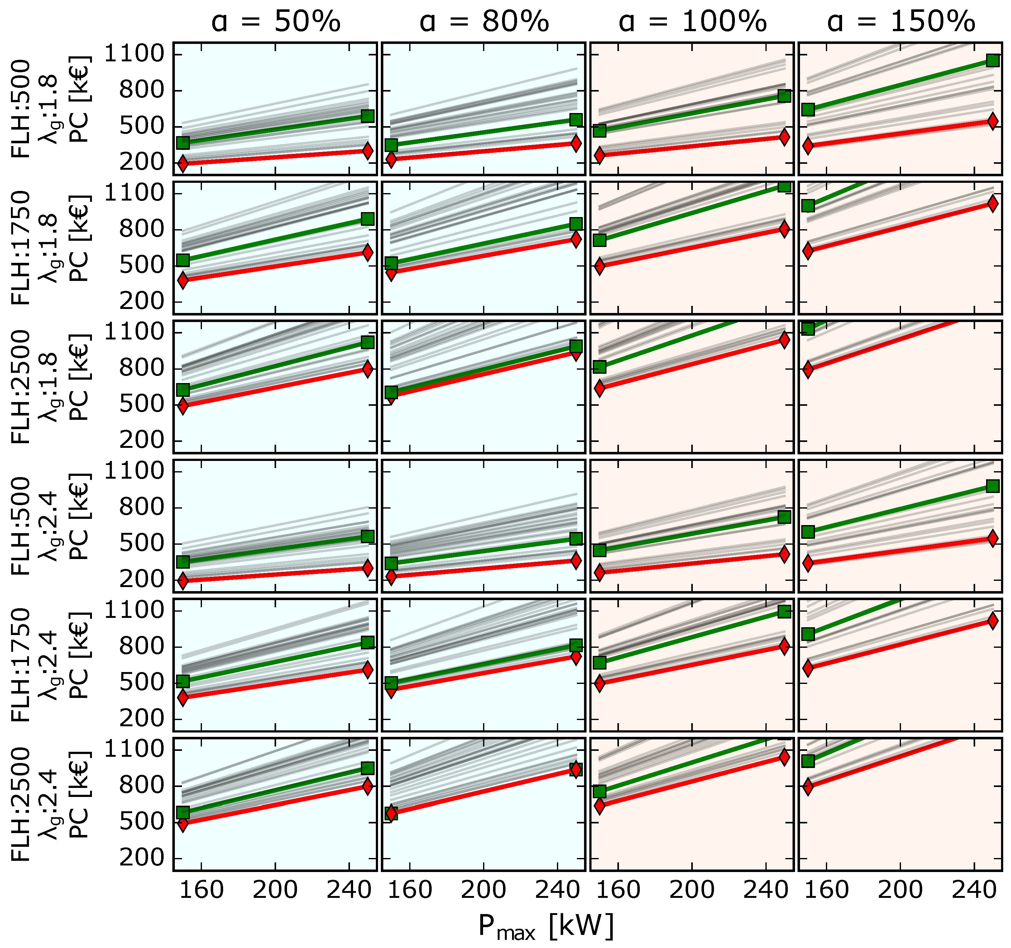
Figure 4.
Present Cost (PC) of HVAC scenarios (Geo-Sce) containing only one heat and one cold production system, each coupled to its own emission system for the different parameter values of Table 4. The blue backgrounds indicate that borefield of the Geo-Sce is heating dominated (more energy extracted than injected). The lines representing GEOTABS-M-Sce are plotted in green with square markers and the lines referring to the most conventional scenario type (Conv-M-Sce) are plotted in red with diamond markers.

Figure 5.
Present Cost (PC , filled markers) and CO emissions (unfilled markers) of HVAC scenarios (Geo-Sce) containing only one heat and one cold production system, each coupled to its own emission system for the different parameter values of Table 4 and kW. Only the GEOTABS (GEOTABS-M-Sce), the most conventional (Conv-M-Sce), the cheapest (M-Sce*) and the cheapest geothermal scenarios (Geo-Sce*) are plotted. The legend specifies the components of the HVAC scenario and the fraction of installed power they cover.

Figure 6.
Heating (left) and cooling curves (right) with triangular (top) and logarithmic (bottom) shapes. The represented cooling curves correspond to the heating curve with kW for different values.
Figure 6.
Heating (left) and cooling curves (right) with triangular (top) and logarithmic (bottom) shapes. The represented cooling curves correspond to the heating curve with kW for different values.

Figure 7.
Present Cost (PC , filled markers) and CO emissions (unfilled markers) of HVAC scenarios (Geo-Sce) containing maximum two heat and two cold production systems, each coupled to its own emission system for the different parameter values of Table 4 but kW, W/m and the Load Duration Curve (LDC) are of triangular shape. Only the GEOTABS (GEOTABS-M-Sce), the most conventional (Conv-M-Sce), the cheapest (M-Sce*) and the cheapest geothermal scenarios (Geo-Sce*) are plotted. The legend specifies the components of the HVAC scenario and the fraction of installed power they cover.
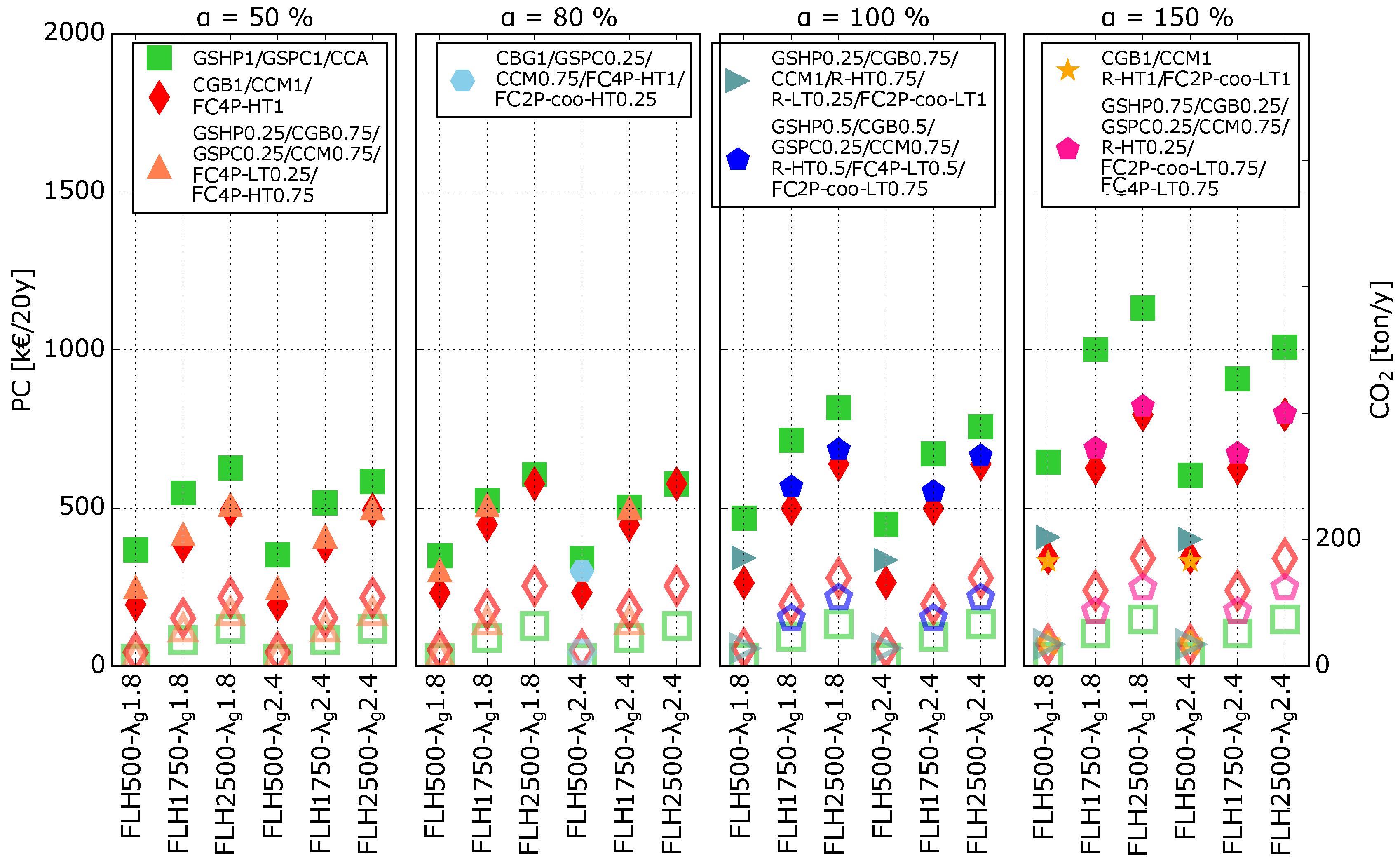
Figure 8.
Same as Figure 7 but W/m.
Figure 8.
Same as Figure 7 but W/m.

Figure 9.
Present Cost (PC , filled markers) and CO emissions (unfilled markers) of HVAC scenarios (Geo-Sce) containing maximum two heat and two cold production systems, each coupled to its own emission system for the different parameter values of Table 4 but kW, W/m and the LDC are of logarithmic shape. Only the GEOTABS (GEOTABS-M-Sce), the most conventional (Conv-M-Sce), the cheapest (M-Sce*) and the cheapest geothermal scenarios (Geo-Sce*) are plotted. The legend specifies the components of the HVAC scenario and the fraction of installed power they cover.

Figure 10.
Same as Figure 9, but W/m.
Figure 10.
Same as Figure 9, but W/m.


Table 1.
Abbreviation (Abb.,) name, cost function with its lower and upper bounds (∞ means that extrapolation is allowed), Maintenance (Maint.) cost in percentage per year of the investment cost and Life Expectancy (Exp.) of each Heating, Ventilation and Air-Conditioning (HVAC) component, currently included in the database.
| Abb. | Component | Cost Function [€] (*1) | Maint. Cost [%/y] | Life Exp. [y] |
|---|---|---|---|---|
| CGB | Condensing gas boiler | kW | 1.5% | 20 |
| GSHP | Ground source heat pump | kW | 3.0% | 20 |
| CCM | Compression cooling machine | kW | 4.0% | 15 |
| GSPC | Plate HEX for passive ground source cooling | kW | 2% (*2) | 20 (*2) |
| GHEX-V | Vertical ground heat exchanger | (*3) m | 0.25% | 50 |
| R-HT | High temperature radiator | kW | 1.5% | 35 |
| R-LT | Low temperature radiator | kW | 1.5% | 35 |
| FC2P-HT-coo | High temperature 2-pipes fan coil unit (cooling) | kW | 4.0% | 15 |
| FC2P-LT-coo | Low temperature 2-pipes fan coil unit (cooling) | kW | 4.0% | 15 |
| FC4P-HT | High temperature 4-pipes fan coil unit (reversible) | kW | 4.0% | 15 |
| FC4P-LT | Low temperature 4-pipes fan coil unit (reversible) | kW | 4.0% | 15 |
| CCA | Concrete core activation | m | 2.0% | 50 |
Table 2.
Efficiencies (i.e the ratio between the useful thermal energy and the used electrical energy) of production components based on values from technical datasheets (TS) and Annex 48 [39]. In the case of Ground Source Heat Pump (GSHP), the given efficiency corresponds to the Seasonal Performance Factor (SPF) assuming a circulation pump power of 2.5% of the heat pump thermal power. The Coefficient of Performance (COP) is given in brackets and it is evaluated for a source temperature of 5 C.
| Efficiencies [-] | |||||||||
|---|---|---|---|---|---|---|---|---|---|
| 30 | 35 | 45 | 60 | 10 | 15 | 20 | [C] | ||
| CGB | 1.06 | 1.06 | 1.02 | 0.98 | - | - | - | (*1) | |
| GSHP | 4.91 | 4.44 | 3.55 | 2.62 | - | - | - | (*2) | |
| (5.60) | (5.00) | (3.90) | (2.80) | ||||||
| GSPC | - | - | - | - | - | 20.00 | 20.00 | ||
| CCM | - | - | - | - | 3.90 | 4.30 | 4.70 | (*3) | |
Table 3.
Parameters of emission components (component abbreviations are explained in Table 1). Nominal conditions are given as with and the supply, return and zone air temperatures. The power ratio column indicates the ratio between cooling and heating powers for reversible systems and the last column introduces a correction factor () for the energy use of the emission system to represent the suboptimality of its control.
| Nominal Conditions (C) | Power Ratio | |||
|---|---|---|---|---|
| Heating | Cooling | Cooling/Heating | (*3) | |
| CCA | 30/-/- | 20/-/- | 125% (*1) | 0.83 |
| FH | 35/-/- | 20/-/- | 30% (*2) | 0.83 |
| HTR | 60/50/20 | - | - | 0.91 |
| LTR | 45/35/20 | - | - | 0.91 |
| FC4P-HT | 60/50/20 | 10/15/25 | 60% | 1 |
| FC4P-LT | 45/35/20 | 15/20/25 | 63% | 1 |
| FC2P-coo-HT | - | 15/20/25 | - | 1 |
| FC2P-coo-LT | - | 10/15/25 | - | 1 |
(*1) It is assumed that CCA can provide a maximum of 40 W/m for heating and 50 W/m for cooling; (*2) It is assumed that FH can provide a maximum of 100 W/m for heating and 30 W/m for cooling; (*3) Taken from NBN EN15316-2-1:2007 [34].
Table 4.
Symbol, units, description and possible values of the different parameters used in Section 6.
Table 4.
Symbol, units, description and possible values of the different parameters used in Section 6.
| Symbol | Units | Description | Considered Values |
|---|---|---|---|
| [kW] | Maximal heating power | ||
| FLHh | [h] | Full load hours (heating) | |
| [%] | Cooling to heating energy ratio | ||
| Ground conductivity | |||
| [W/m] | Maximum heating power per floor surface area | [27, 70 (*1)] |
(*1) this value is only used in Section 6.2, not in Section 6.1.
Table 5.
Description of the abbreviations used in Section 6. When the abbreviation is followed by a star (*), it indicates that the scenario is cost optimal compared to the scenarios of the same type.
Table 5.
Description of the abbreviations used in Section 6. When the abbreviation is followed by a star (*), it indicates that the scenario is cost optimal compared to the scenarios of the same type.
| Abbr. | Description |
|---|---|
| Sce | HVAC scenario(s) containing some heat/cold production and emission systems. |
| M-Sce | Minimal Sce: Sce containing only one heat, one cold production system, each coupled to its own emission system. (*1) |
| H-Sce | Hybrid Sce: Sce containing max two heat and max two cold production systems, each coupled to its own emission system. (*1) |
| GEOTABS-M-Sce | M-Sce only composed of GSHP/GSPC/CCA. |
| Conv-M-Sce | Conventional M-Sce only composed of CGB/CCM/ FC4P-HT. |
| Geo-Sce | Sce with at least one geothermal production system. |
(*1) In case of reversible emission system, one heat and one cold production system can be coupled to the same emission system.
© 2018 by the authors. Licensee MDPI, Basel, Switzerland. This article is an open access article distributed under the terms and conditions of the Creative Commons Attribution (CC BY) license (http://creativecommons.org/licenses/by/4.0/).
Share and Cite
MDPI and ACS Style
Picard, D.; Helsen, L. Economic Optimal HVAC Design for Hybrid GEOTABS Buildings and CO2 Emissions Analysis. Energies 2018, 11, 314. https://doi.org/10.3390/en11020314
AMA Style
Picard D, Helsen L. Economic Optimal HVAC Design for Hybrid GEOTABS Buildings and CO2 Emissions Analysis. Energies. 2018; 11(2):314. https://doi.org/10.3390/en11020314
Chicago/Turabian StylePicard, Damien, and Lieve Helsen. 2018. "Economic Optimal HVAC Design for Hybrid GEOTABS Buildings and CO2 Emissions Analysis" Energies 11, no. 2: 314. https://doi.org/10.3390/en11020314
Note that from the first issue of 2016, this journal uses article numbers instead of page numbers. See further details here.