Dynamic Analysis of a Hybrid Energy Storage System (H-ESS) Coupled to a Photovoltaic (PV) Plant

Abstract

Nowadays energy storage is strongly needed to allow grid safety and stability due to the wide penetration of renewable plants. Mainly economic and technological issues impede a relevant integration of conventional storage devices in the energy system. In this scenario, the hybridization of different storage technologies can be a techno-economic solution useful to overcome these issues and promote their diffusion. Hybridization allows multi-operation modes of the Energy Storage System (ESS), merging the positive features of base-technologies and extending their application ranges. This paper provides a dynamic analysis of a hybrid energy storage system (H-ESS) consisting of a flywheel and a battery pack coupled to a photovoltaic generation plant and a residential load up to 20 kW. A dynamic model of the overall micro-grid (MG) was developed implementing the H-ESS preliminary sizing and a suitable management algorithm. The instantaneous behavior of each component was evaluated. A brief summary of the MG performance at different weather and load conditions was provided together with a characterization of the impact of power fluctuations on the battery current and on the power exchange with the grid.

1. Introduction

Recent studies on renewable energy sources (RES) show complexity in controlling and offsetting over and under production events [1,2]. As described in [3], the main limitations of RES are due to their intermittent and fluctuating behaviour, especially for solar and wind power plants. For these reasons, RES are defined as non-programmable energy sources that negatively affect the stability and safety of the electric grid [4]. In fact, thermal power plants, with particular reference to combined cycles fed by natural gas, are forced to compensate continuously their power variations avoiding network imbalances. In particular, the conventional power plants cycling leads to a significant deterioration in their overall performance (e.g., efficiency, wear) [5,6,7,8,9].

Synchronization of network reserves and ESS integration in the electric grid can be seen as two effective and complementary solutions to overcome the above-mentioned RES technical limits. This is consistent with the objectives of the IEC T120 work program [10], where Energy Storage Systems (ESSs) are identified as a solution to efficiently deliver sustainable, economic and secure electricity supplies. Indeed, as discussed in [11,12,13], thanks to their excellent skills in terms of scalability and efficiency, ESSs represent one of the best solutions available for a better RES exploitation and penetration. Specifically, the most interesting energy storage technologies suitable to achieve RES penetration targets set by the EU (European Union) are presented in [11]. An interesting review is provided in [14] where the current technology readiness level of various ESS technologies is analysed.

In this context, the importance of storage systems also in micro-grids (MGs) to extend the RES penetration, especially in remote and rural areas, has to be carefully analyzed. A MG can be defined as “a network of low voltage power generating units, storage devices and loads capable of supplying a local area such as suburban area, an industry or any commercial area with electric power and heat” [15]. Therefore, an innovative systemic solution can be the integration of different energy storage systems into micro-grids that will permit to overcome the intrinsic limitations of individual storage technologies. In fact, in order to achieve future aims about the reduction of the greenhouse gas emissions and polluting species, future electricity network should be reliable, flexible, accessible and economically viable [16].

Flywheels represent a specific energy storage technology [12]. They can provide power in short time applications and are characterized by long lifetimes, high efficiency and fast response [17]. Flywheels are often used to reach energy quality and stability improvement [18,19,20], power smoothing [21], renewable energies integration support [22,23].

In the technical literature, several studies using flywheels in mobile applications are presented [24,25]. In particular, an in depth discussion about ESS for electric vehicle applications is provided in [26]. Moreover, broad comparative reviews of ESS for stationary applications are presented in [27,28]. In particular, in [29] an interesting solution, for residential applications, composed by a hybrid generation system was analysed. Specifically, it consists of a PV (photovoltaic)-wind power plant coupled with a flywheel-based storage system, aiming to clipping grid consumption by optimizing the RES exploitation. So dynamic power management strategy and algorithm were developed with the purpose to achieve a controlled power output in a generation stochastic system.

The integration of flywheels in wind power plants is also discussed in [30]. Specifically, a solution to maximize the extracted power characterized by a stochastic behavior, by coupling a flywheel with a wind generator is presented. The same authors in [21] highlighted the smoothing function of the flywheel in wind generation applications.

Flywheel hybridization with other technologies characterized by higher energy capacity can extend their application range. At the same time, hybridization provides, mainly thanks to the fast response of flywheels, beneficial effects towards the other base technologies. If batteries are considered, the potential enhancement of their duration due to the flywheel peak shaving function is highlighted. Currently, only one large-scale hybrid storage plant is planned thanks to a EU’s Horizon2020 project [31], while relative to small-sized plants only in [32] is the flywheel-battery hybrid configuration is addressed. Anyway, the management strategy is not described and the dynamic modelling and analysis of operating modes along the year are not investigated for both battery pack and flywheel.

For the above reasons, the present work aims to fill this gap providing a dynamic analysis of the power flow interaction among the components of a micro-grid (MG) characterized by a flywheel-battery hybrid storage system (H-ESS) coupled with a PV plant and a complex user load. In the investigation of the H-ESS behaviour also the environmental conditions under which the RES plant operates are taken into account.

In the chosen architecture, the battery pack is the main energy storage system while the flywheel has a peak shaving function. In particular, as anticipated, in order to investigate the dynamic interaction among the components of a micro-grid, a dynamic model was developed in the Matlab Simulink environment. Also a power flow management strategy was configured, in order to maximize the MG energy independence from the grid, and implemented in the Simulink model. Simulations were carried out under different operating and weather conditions to evaluate the energy performance of the MG and to characterize the dynamic interaction among plant devices and their working profiles. Simulations results, which will be the basis of further developments of plant components, confirm the flywheel peak shaving function, rising the quality of the battery exchanged current and of the power exchanged with the grid.

2. Micro-Grid Layout

The electrical architecture of the micro-grid here studied was picked out by comparing several alternatives among those proposed in the literature. In [33] different architecture models of the MG, with their advantages and disadvantages, were analysed. Also in [34] and [16] a performance comparison of Alternating Current (AC), Direct Current (DC), hybrid AC-DC micro-grids and other configurations was realized. In particular, in [16] authors assert how DC distribution systems present less power quality problems.

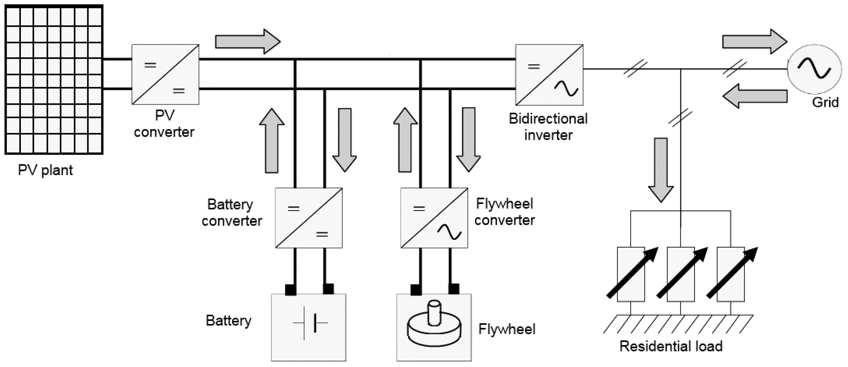
In this context, the architecture here analysed, depicted in Figure 1, can be divided into four sections: “Photovoltaic plant”, “Battery storage system”, “Flywheel storage system” and “Residential load”. Each parallel branch is connected to a common DC bus at 400 V_DC rated voltage. All branches interact with an inverter which brings the voltage conditions to those typical of residential users. DC/DC and AC/DC converters, with their efficiency and response delay, are not implemented in this dynamic model yet.

As said in the Introduction, in this configuration, the battery is the primary energy storage system and the flywheel helps in the load peak-shaving, providing or absorbing power peaks and reducing fluctuations of power from/to battery and grid.

Regarding the MG sizing, in a previous study [35], according to a multi-criteria sensitivity analysis on yearly base, PV plant, battery and flywheel sizes have been fixed. Specifically, a PV plant with a peak power of 11 kW, a battery of 10 kWh (a lithium iron phosphate pack is modelled in the present study) and a mechanical flywheel of 11 kW of maximum power and 2 kWh of capacity were identified.

The chosen PV plant size, as the others analyzed in [35] up to 20 kW, is compliant with the standard size of Italian plants. Indeed, at the end of 2016, about 91% of PV installed plants results in the power range up to 20 kW [36]. Consequently, in consideration of the PV sizing a complex residential load was selected.

3. Load Profile Analysis and Micro-Grid Dynamic Modelling

As mentioned in the Introduction, the Simulink dynamic model has allowed to simulate and, subsequently, analysed the MG operation at various working points. In particular, thanks to the dataset implemented, the dynamic model can reproduce the photovoltaic plant production for a chosen day, taking into account of seasonal and meteorological effects. At the same time, the model permits to evaluate the operative conditions of the hybrid storage system, in term of battery state of charge (SOC) and flywheel angular velocity. In the load management strategy, the above parameters (PV produced power, battery and flywheel SOC) are used in order to minimize the withdrawal from the electrical network. Figure 2 reports a global overview of the MG dynamic model.

As mentioned in the description of MG layout, the model was essentially divided into four interconnected blocks: “Load”, “Flywheel”, “Battery” and “Control Logic” (including QB block). In the “Load” section, the instantaneous power difference between current PV production (referred to a location in Central-Southern Italy) and load demand is calculated. This time dependent signal is central to understanding the MG operative functions. When it assumes a positive value, a surplus in energy production occurs together with the possibility to storage it in the hybrid ESS, according to the current energy and power limits. Vice versa, a negative value is indicative of a lack in PV production with respect to the load demand, which implies a power demand from the hybrid ESS. In the follow, the singular sections of the MG model are described.

3.1. Load Section

The user load demand was based on a measurements based dataset presented in [37]. Experimental data were sampled continuously for two years by 20 homes, with intervals of 8 s. The implemented residential load takes into account of programmable and non-programmable loads.

In this study the load relative to a complex residential user made up of three houses was considered. Specifically, a summer and a winter (Figure 3) daily profiles were extracted.

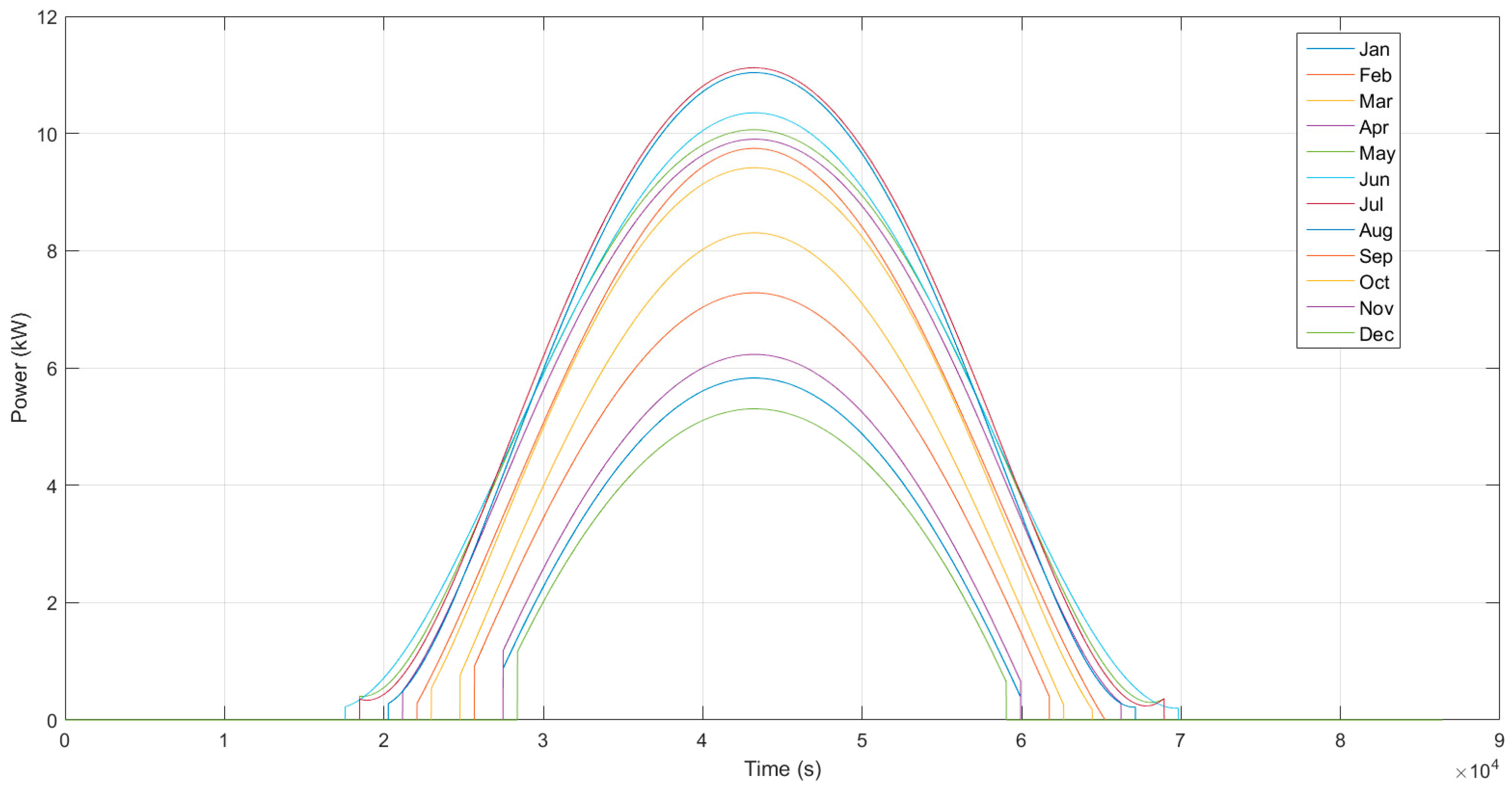
Concerning the renewable production, the photovoltaic power generation profile implemented in the model refers to a location in the Central-Southern Italy, with south facing panels with a tilt of 30°. Figure 4 shows the average monthly production for 11 kW PV plant.

As anticipated in the introduction, also the weather conditions for the evaluation of the PV production were taken into account. In particular four different meteorological conditions were considered through the implementation of the following mitigation coefficients [38]:

• 0%: no production, day with total cloud cover.
• 30%: very cloudy with temporary clear up.
• 50%: day with variable cloudiness.
• 100%: maximum production, clear sky.

3.2. Battery Model

In order to implement the most MG’s capabilities, an integrated dynamic model of the battery pack was developed to analyse its transient operation. In this model it was also evaluated how much power is possible to store or deliver to the MG.

Authors in a previous research works [39] have tuned the model for a Q (Ah) capacity battery with which the battery SOC (state of charge) was calculated taking into account battery datasheet characteristics. Specifically, the open circuit voltage (V_ocv), the change of internal resistance ($R_{bat}^{\mathrm{int}}$) during charging (R_ch) or discharge (R_dis) were used to characterize the battery behaviour.

Usually battery current (I_bat) and voltage (V_bat) can be characterized as:

$$I_{bat}=\frac{V_{ocv}-\sqrt{V_{ocv}^2-4R_{bat}^{\mathrm{int}}P}}{2R_{bat}^{\mathrm{int}}}$$

(1)

$$V_{bat}=V_{ocv}-R_{bat}^{\mathrm{int}}{I}_{bat}$$

(2)

where P is the power required/delivered to the battery and:

$$V_{ocv}=\left\{\begin{array}{ll}{V}_{ocvc}=f_1(SOC)& \mathrm{charge}\\ V_{ocvd}=f_2(SOC)& \mathrm{discharge}\end{array}\right\}$$

(3)

$$R_{bat}^{\mathrm{int}}=\left\{\begin{array}{ll}{R}_{ch}=f_3(SOC)& \mathrm{charge}\\ R_{dis}=f_4(SOC)& \mathrm{discharge}\end{array}\right\}$$

(4)

The Equations (3) and (4) were implemented by using look-up tables based on experimental data. In [39] the V_ocv trends of the LFP (Lithium iron phosphate) battery together with its internal resistance are shown. The determination of SOC was carried out as follows:

$$SOC=SO{C}_{ini}-{\displaystyle \int \frac{\eta I_{bat}}{Q}}$$

(5)

and:

$$\eta =\left\{\begin{array}{ll}{\eta }_{ch}=\frac{V_{ocv}}{V_{ocv}-I_{bat}{R}_{ch}}& \mathrm{charge}\\ {\eta }_{dis}=\frac{V_{ocv}-I_{bat}{R}_{dis}}{V_{ocv}}& \mathrm{discharge}\end{array}\right\}$$

(6)

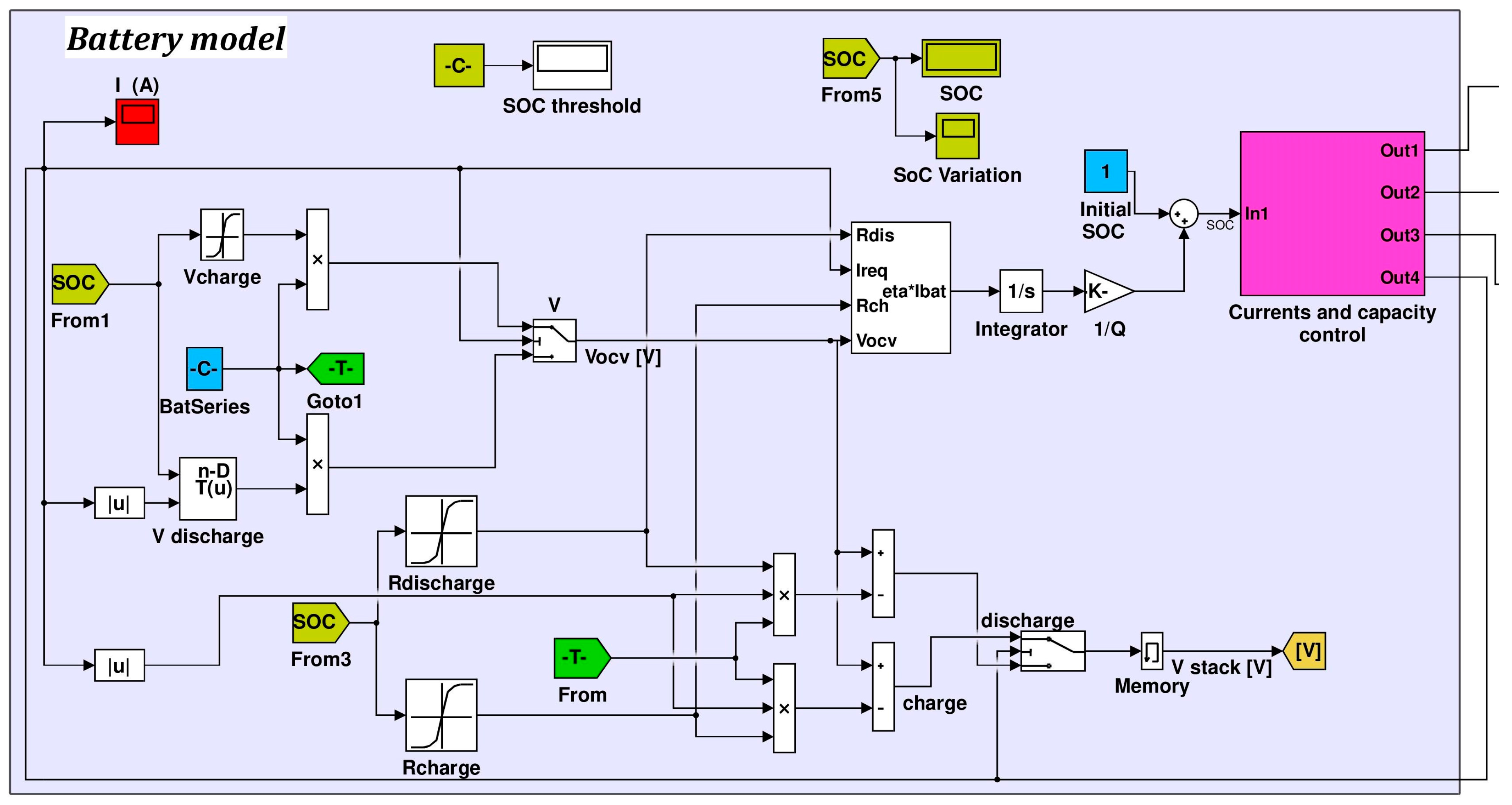
where SOC_ini is the initial value of SOC and Q (Ah) represents the battery capacity. In the present study battery capacity was set at 79.4 Ah (five modules in series) with a nominal storage power of about 10 kWh.

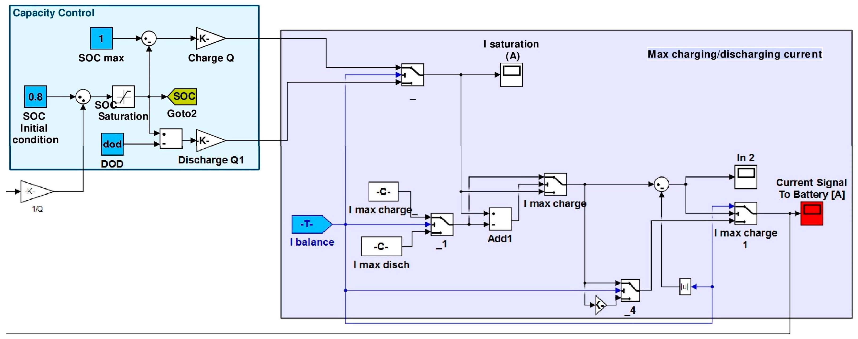
The Simulink battery model is shown in Figure 5. Specifically, the curves shown in [39] were implemented in the V_charge, V_discharge, R_charge and R_discharge blocks. In the “Current and capacity control” section (Figure 6) the current demand I_batt (out4 in Figure 5) was compared with the maximum charge/discharge (82/200 A) current as well as the instantaneous SOC. Therefore if I_batt exceeds the power and/or energy limits, the exceeding current was delivered/requested to the grid.

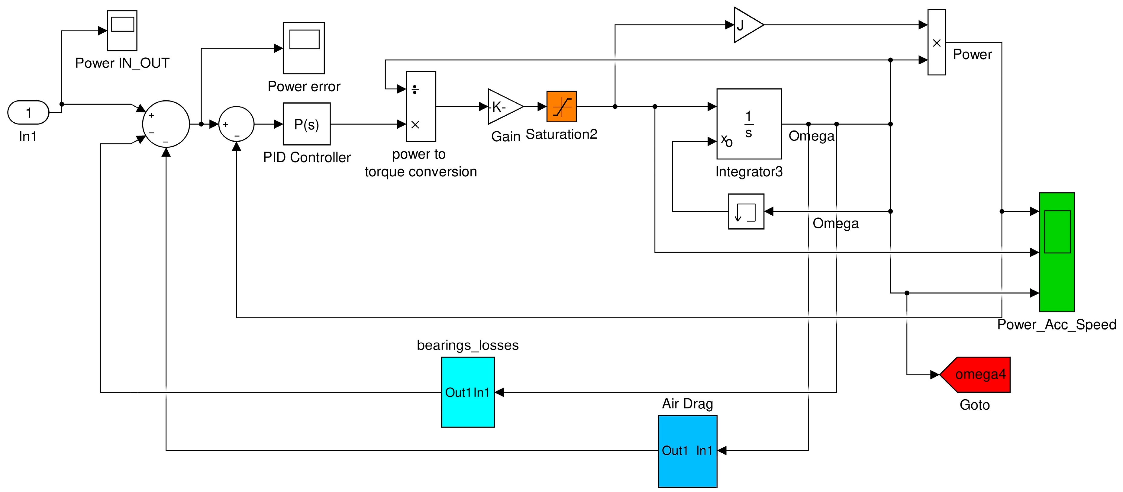
3.3. Flywheel Model

According to [23], a flywheel is able to store energy in the form of kinetic energy, rotating around its axis, and to quickly respond to energy peaks demand. Thanks to these features, in the MG model here presented, flywheel works in peak-shaving mode extending the battery lifetime.

Equations (7) and (8) show flywheel power P and shaft torque T, as reported in [25]:

$$P=T\omega$$

(7)

$$T=J\dot{\omega }+T_d+T_b$$

(8)

where: J is the rotational inertia, T_b denotes the frictional torque due to bearings, $T_d$ is the aerodynamic drag torque, $\dot{\omega }$ is the angular acceleration.

Mathematical models concerning mechanical (friction) and aerodynamic losses useful for the model development can be found in [40,41]. The power losses associated with the mechanical bearings are quantifiable by the following Equation (9):

$$P_{b,loss}=1.05\times {10}^{-4}M$$

(9)

where $P_{b,loss}$ indicates the power losses, $n$ denotes flywheel rotational speed and $M$ is the total bearing frictional moment, as detailed in [41].

Aerodynamic losses can be calculated by the following Equations (10) and (11):

$$P_w=M_C\omega$$

(10)

$$M_C=C_f\rho \pi {\omega }^2{r}^{4}L$$

(11)

In Equation (10) aerodynamic power losses are linearly related to windage frictional moment (M_C) and to flywheel rotational speed (ω). M_C for cylindrical flywheel is expressed by Equation (11), known cylinder torque coefficient $C_f$, fluid density $\mathsf{\rho }$ and the geometric features of the cylinder (i.e., radius r and length L). It is remarked that, in the investigated system, aerodynamic drag is negligible since the system is kept under vacuum.

The flywheel was modelled in the Simulink environment (Figure 7) implementing the following technical data:

• Max Power (kW): 11
• Energy (kWh): 2.1
• ω (rad/s): max 1131, min 314
• Radius (m): 0.4
• Length (m): 0.08
• Weight (kg): 160.6
• Material: Steel

The model input is a power load signal (In1). If this signal is negative, it corresponds to a power request, vice versa, to a power supply. The model provides as outputs the exchanged power with the grid and the battery, flywheel rotational speed and its angular acceleration.

On the basis of experimental data, the parameters of Equations (9)–(11) were evaluated and implemented in “bearing losses” and “air drag” subsystems (in light blue and blue, respectively) to determine mechanical and aerodynamic losses.

3.4. Models Integration

The integration of model sections was carried out according to Figure 2. Specifically the model core is the “Control Logic” block where the main output of the other subsystems are elaborated and used to determine the MG power flows. In particular the input parameters needed by the “Control Logic” subsystem are:

• “omega”: flywheel instantaneous angular speed. It is an output of “Flywheel” block.
• “diff”: difference between the electric load required by the user and the photovoltaic production. These signal can represent a power lack or surplus. It is an output of “Load” block.
• “P_pv”: photovoltaic instantaneous production. As the previous one, it is determined in “Load” block.
• “SOC”: instantaneous state of charge, determined in “Battery” subsystem.
• “qb” and “qb2”: two parameters determined in “QB” block on the basis of the difference values (the current one and the one relative to the previous calculation time step) between production and load. These parameters approximate the trend of “diff”, by excess or defect respectively (with reference to absolute values), according to step profiles characterized by a slow variation. In the follow a brief discussion on these parameters is provided.

The above listed parameters are elaborated in the “Control Logic” subsystem to define the energy amounts processed separately by the battery and the flywheel (“batt” and “Envol” output signals). These two values are directly sent, as input, to the “Battery” and “Flywheel” blocks.

4. Micro-Grid Management

As just anticipated above, the MG management was implemented in the Simulink model through a Matlab code in the “Control Logic” block. The designed management strategy of the MG (flowcharts are provided in Figure 8 and Figure 9) starts by evaluating the instantaneous difference between P_R (production from renewable) and P_L (power required by the electric load); subsequently, the two main cases can be distinguished:

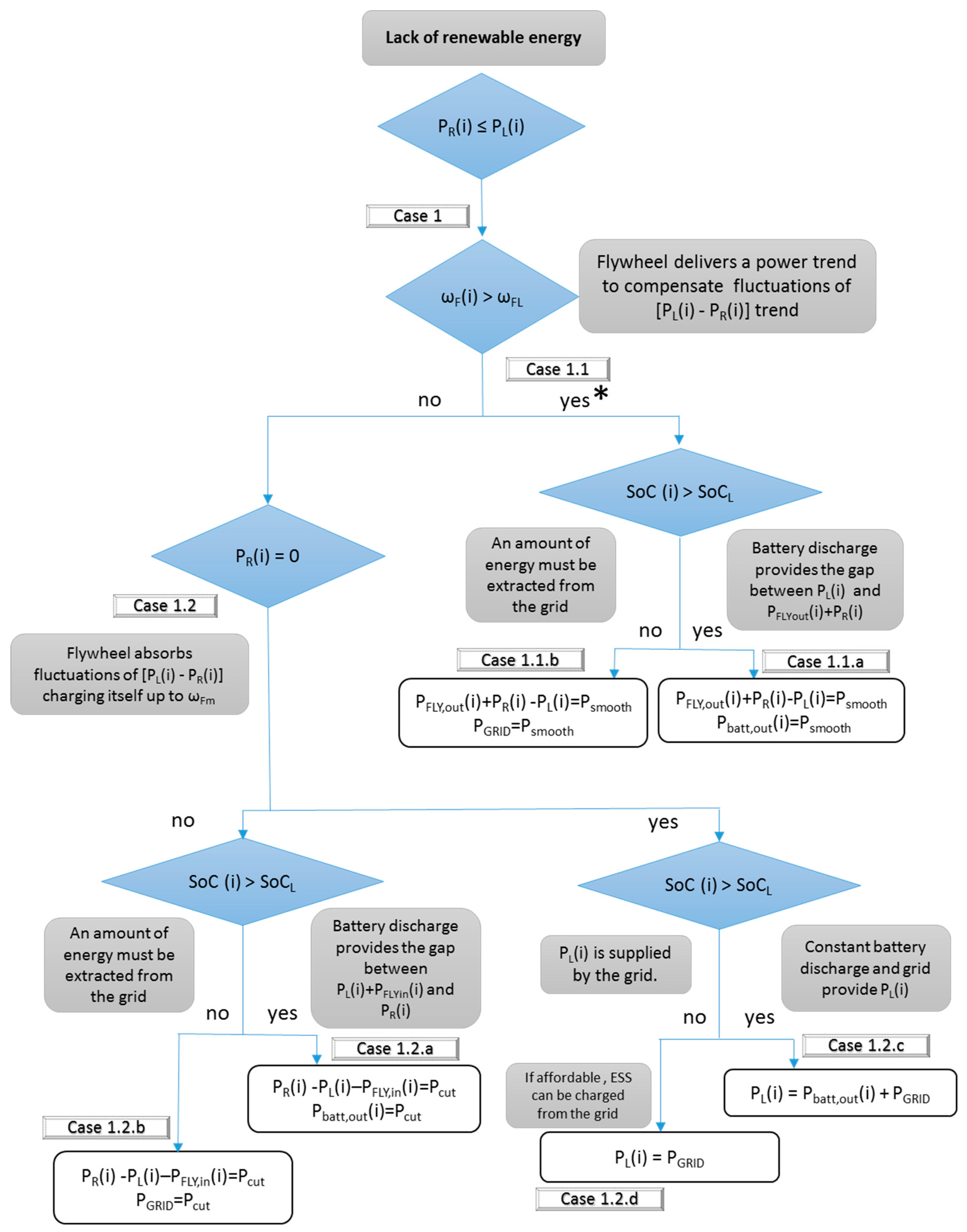
• CASE 1: Diff = P_R (i) − P_L (i) ≤ 0:

The renewable plant production is not sufficient to satisfy the electrical load and the flowchart of Figure 8 is followed; additional conditions (mainly battery state of charge, flywheel rotational speed, absence of PV production) lead to the identification of different sub-cases (1.1a, 1.1b, 1.2a, 1.2b, 1.2c and 1.2d).

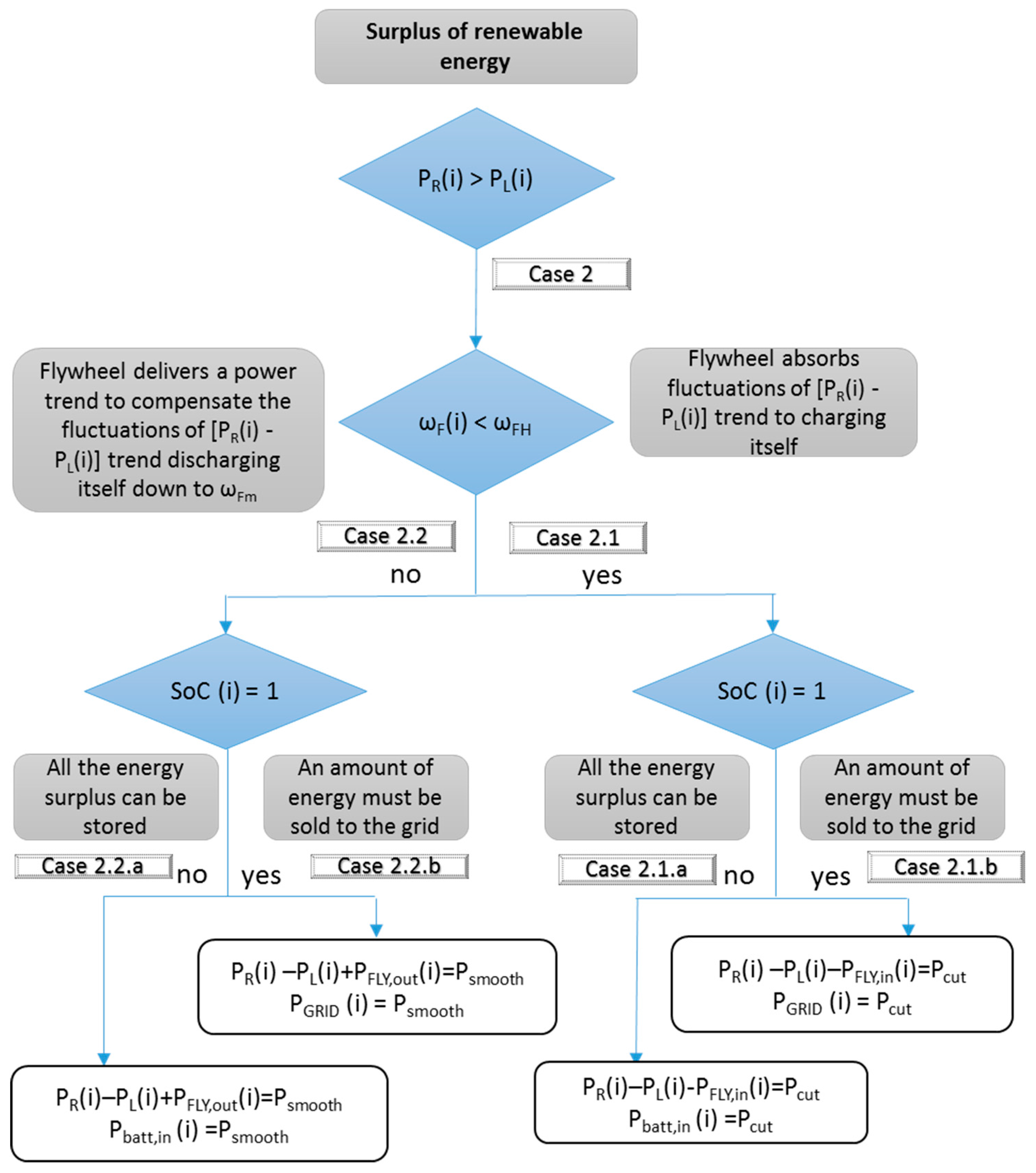
• CASE 2: Diff = P_R (i) − P_L (i) > 0:

There is a surplus of renewable production and the flowchart of Figure 9 is followed activating at each time step one of the 2.1a, 2.1b, 2.2a and 2.2b sub-cases.

In the following a brief discussion of all operating cases is done.

- Case 1.1

The difference between production and load assumes a negative value (lack of production, Diff < 0), so if the flywheel is capable to deliver energy (rotational speed greater than the minimum threshold ω_min) the software enters in sub-case 1.1. Moreover, after evaluating the battery SOC, one of the cases 1.1a (battery state of charge greater than the minimum limit, SOC > SOC_L) and 1.1b (the battery is not capable to deliver energy) is chosen.

In case 1.1a the difference between the energy produced by the renewable plant and energy required by the load is supplied partly by the battery, while the flywheel provides the amount to dampen load peaks. In the case the storage system is not able to completely satisfy the load, energy can be drawn also from the grid. In 1.1b the battery is discharged. Therefore, energy is partly provided by the grid and the flywheel releases the energy amount to provide a peak-shaving function towards the grid.

- Case 1.2

Also in this case, there is a lack of production, but the flywheel has already reached the minimum rotational speed ω_min. Depending on the energy renewable production and battery SOC, cases 1.2a (PR > 0 and battery able to deliver, SOC > SOC_L), 1.2b (PR > 0 and discharged battery), 1.2c (PR = 0 and SOC > SOC_L) and 1.2d (PR = 0 and discharged battery) can be detected.

In case 1.2a the renewable plant delivers energy. The battery supplies an energy amount, necessary to cover the electrical load increased of a share of energy relative to the oscillations absorbed by the flywheel. Thus, the flywheel is charged and increases its rotational speed starting from ω_min. This operation mode is aimed to guarantee a more constant profile of energy demand required to the battery.

In case 1.2b battery is discharged. Consequently, the grid supplies the energy amount to guarantee the complete satisfaction of the electric load and to partly recharge the flywheel. So, a peak-shaving function is provided towards the grid.

If RES production is zero the case 1.2c occurs where the electrical load request is covered by using the battery and the grid. The flywheel, considering the energy losses, progressively reduces its rotational speed under ω_min up to its stopping.

Finally, case 1.2d is characterized by no RES production and battery SOC equal to the minimum one. Therefore, the electrical load is satisfied by the grid, while the flywheel progressively reduces its rotational speed below its minimum rotational speed in order to avoid energy withdrawal to cover energy losses.

- Case 2.1

In this case a PV production surplus occurs. The flywheel is not fully charged (ω < ω_max) and, in relation to the battery SOC, it is possible to distinguish:

Case 2.1a with battery not fully charged: the surplus energy is stored both in battery and flywheel. Flywheel absorbs the fluctuations to provide an almost constant charging profile to the battery.

Case 2.1b with battery fully charged: flywheel absorbs energy fluctuations to deliver a constant energy profile to the grid.

- Case 2.2

In case 2.2, in the presence of a PV production surplus, the flywheel is saturated since it is already at its maximum rotational speed. In case the battery has a SOC < SOC_L (2.2a) an amount of energy is stored by the battery, since the flywheel releases to the battery the oscillations reducing its rotational speed. In this way the battery is operated under an almost constant charging profile. In case 2.2b, instead, because the battery is already fully charged, RES production is directed towards the grid. Specifically, the flywheel releases the oscillations towards the grid.

In all cases, energy fluxes processed by storage devices are reduced if not compatible with their energy and power capabilities.

5. Simulation Results

In this section, the simulation results of the analyzed MG are presented. In particular, taking into account of the variation of daily weather conditions and of the seasonal load demand, the battery and flywheel dynamic behaviors were determined. The time step used for daily simulation was set equal to 1 s.

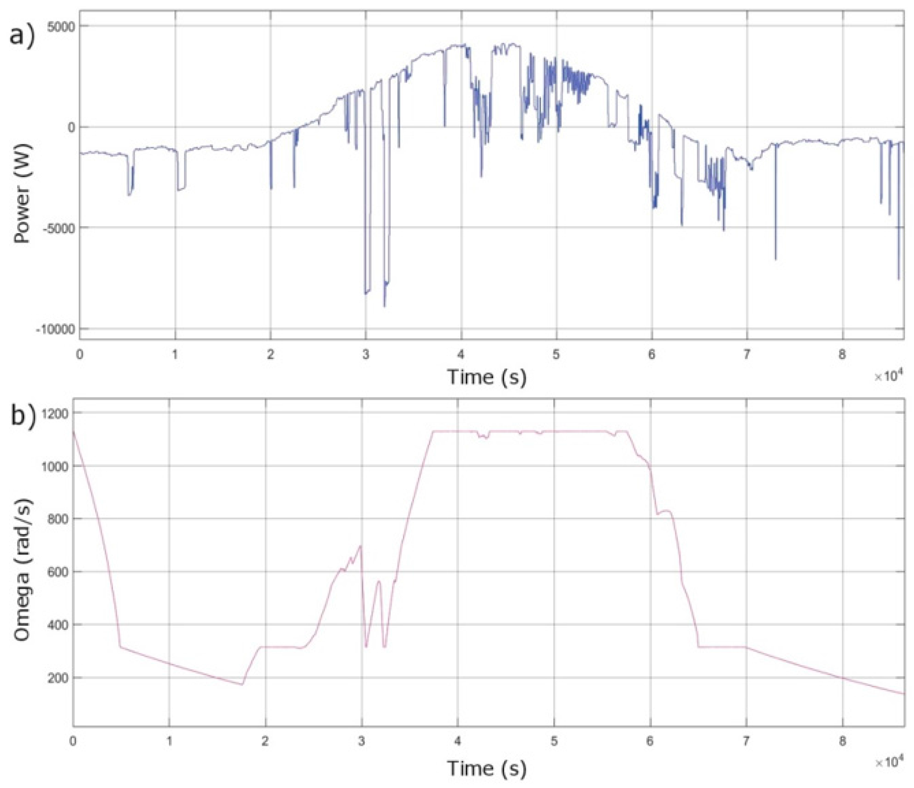
In order to improve the clarity of this section, only the results relating to the summer working operation (in terms of load demand and irradiation) and three weather conditions (100%, 50% and 30% of the nominal irradiation) are presented below. Aiming to appreciate the H-ESS daily performance, its initial condition was set as “fully charged”. This hypothesis is arbitrary and it is not representative of the actual conditions. The simulations, based on the actual load and the PV production profiles of a generic day, aim to analyze the dynamic interactions among MG components and with the grid (evaluating the beneficial effects of hybridization), without evaluating the MG energy performance. 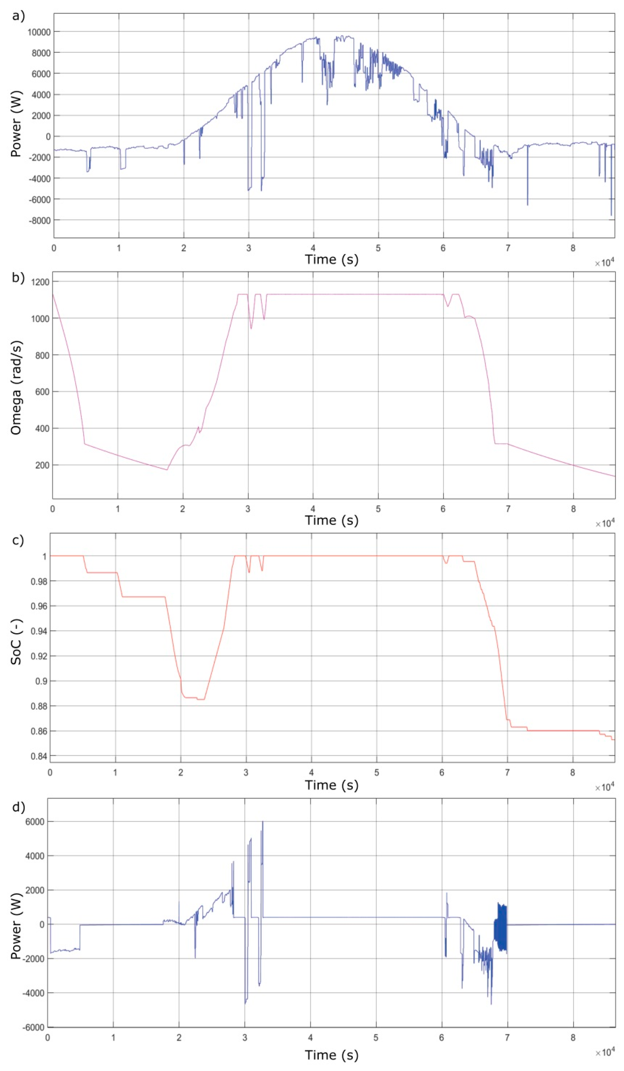To this last purpose, studies have already been conducted by the authors [35] on a yearly basis, leading to the sizing of the MG components. In the following figures, simulations results are shown in the order below:

(a)

the difference between PV production and load demand;

(b)

flywheel angular velocity (index of its state of charge);

(c)

battery SOC;

(d)

flywheel instantaneous exchanged power respectively.

It is emphasized that seconds were chosen as time unit because the studied phenomena are characterized by fast variations. However for clarity in each simulation 0 s stands for the day midnight, 43,200 s for midday and 86,400 for the next midnight.

Figure 10 shows the simulation results for a summer load profile with a completely clear sky (maximum PV production). At the simulation beginning the user load demand is totally covered by the H-ESS as the PV production is zero. Consequently, battery SOC and flywheel angular velocity fall down respectively to about 89% and 200 rpm (the flywheel is left free to rotate under the minimum angular velocity). With the start of PV production, the difference between production and energy demand becomes positive and the storage systems begins to charge up to 100%.

It is emphasized as in the case of extremely high demand peaks (at around 30,000 s of simulation, Figure 10a), storage devices react in a coordinated manner (Figure 10b,c) supplying energy while respecting the control logic, maximizing H-ESS lifetime and effectiveness.

As for the initial part of the simulation, after the sunset, the load demand is covered by battery and flywheel until the first reaches its minimum daily charge state (about 85%), while the second is fully discharged.

It is interesting to make a clarification regarding the power exchanged and provided by the flywheel. As it can be seen in Figure 10d, the flywheel, even when it is fully charged (constant velocity in Figure 10c) contrary to the battery, always needs of a small amount of energy to balance out the bearing losses. For this reason, only when a flywheel its totally discharged and it is left free to rotate under the minimum angular velocity, its power exchange is zero.

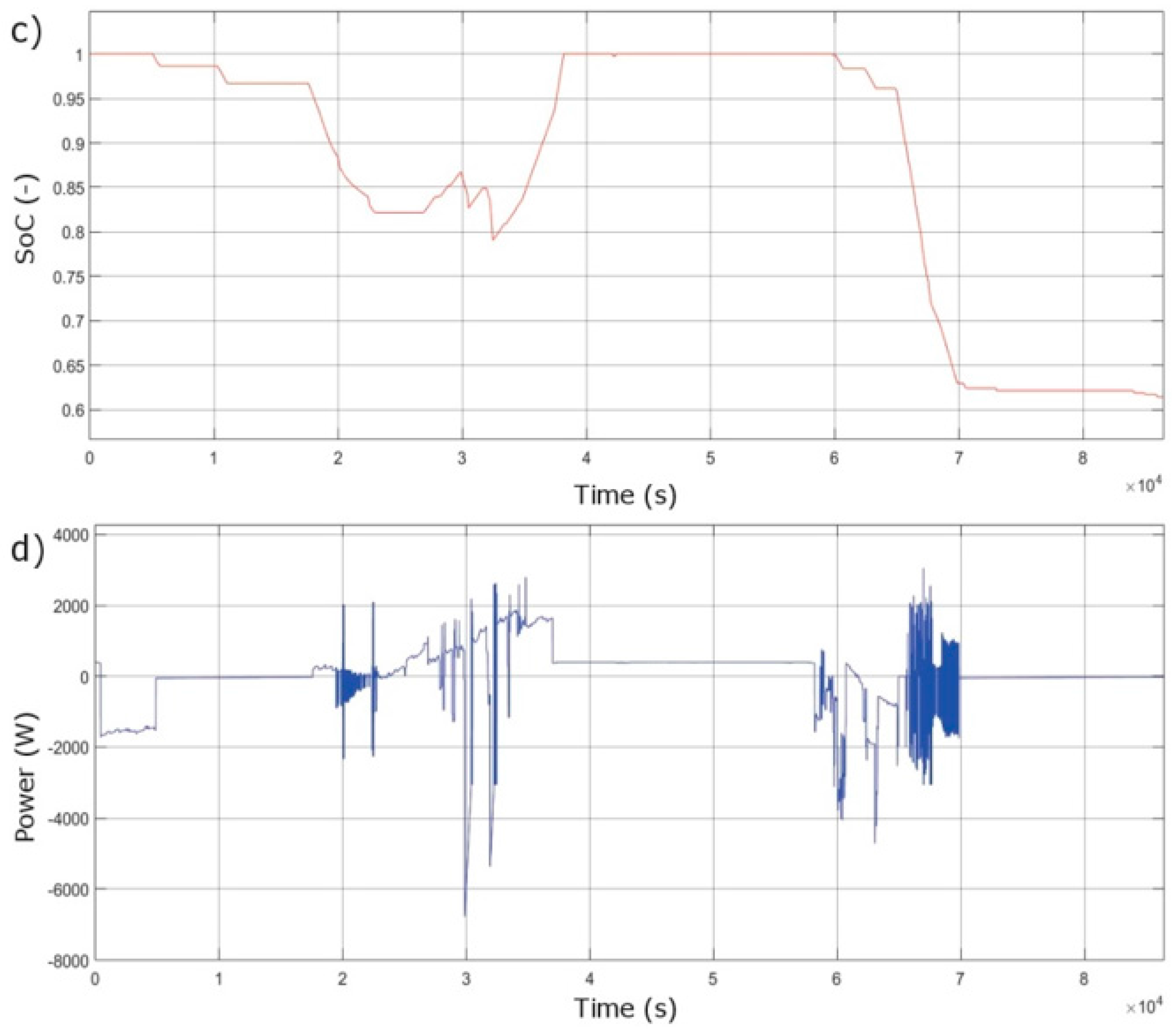
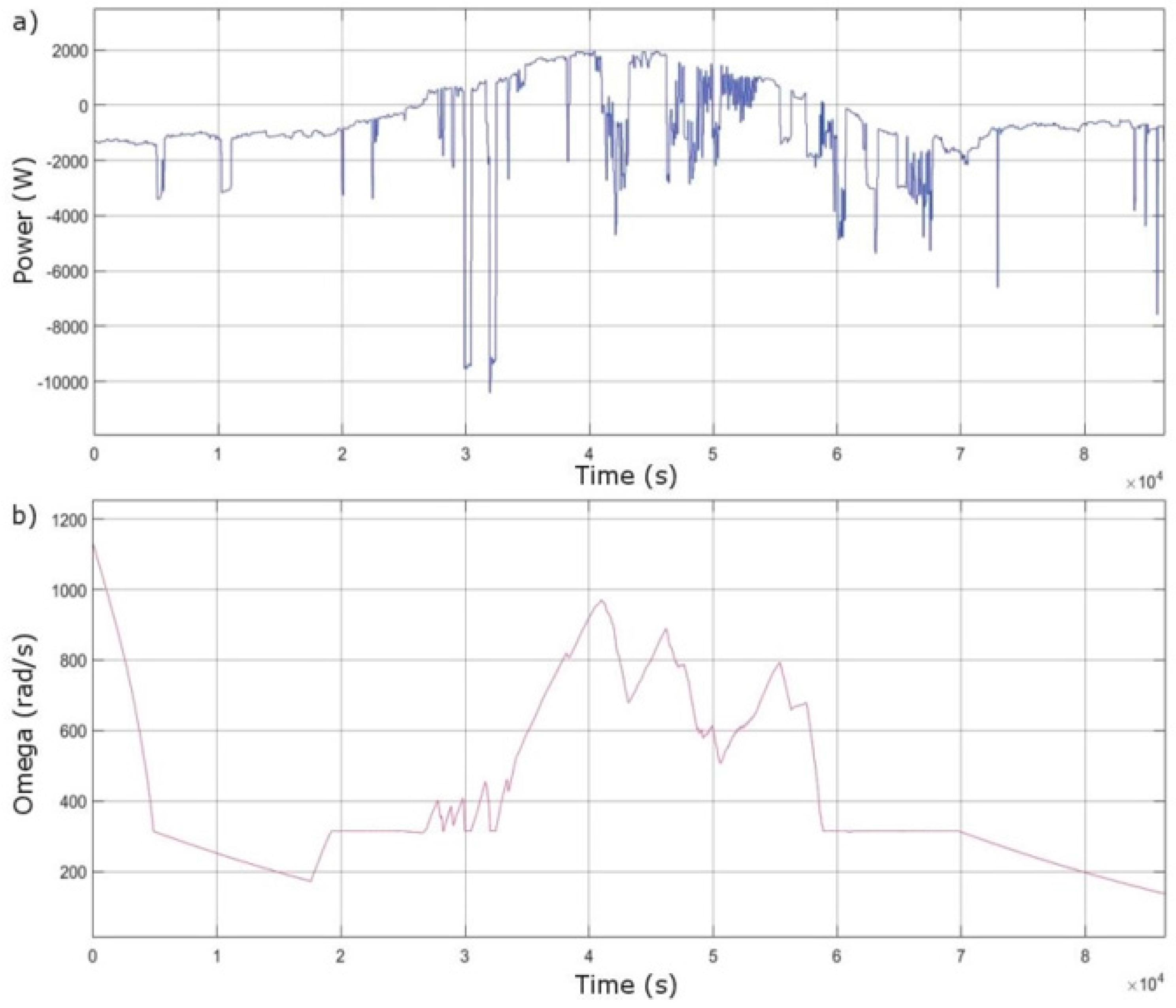
Figure 11 and Figure 12 show respectively the MG operating modes with a RES production characterized by an irradiation equal to 50% and 30% of the nominal one. As it can be seen, lowering the photovoltaic production, a greater exploitation of the stored energy occurs. At the beginning of simulation, as in the nominal case, H-ESS covers totally the users load demand. Then, when RES production begins, the difference between photovoltaic power and load demand becomes positive (panel a in Figure 11 and Figure 12). As the irradiation decreases, this condition occurs more and more later in the time. During the day, the difference surplus sent to H-ESS (maximum power at 40,000 s of simulation), in case of 30% irradiation, is not enough to increase the charge level of the flywheel and battery up to the maximum SOC while it is sufficient for 50% irradiation. During daytime hours, the minimum state of charge of flywheel and battery corresponds to the high demand peaks at about 30,000 s of simulation (i.e., respectively, 314 rad/s and 78% for 50% irradiation and 314 rad/s and about 52% for 30% irradiation). Indeed, as seen in Figure 12b,c), the battery and flywheel never reach their maximum storage capacity during the day, because the PV production is only used to cover the load required by residential utilities and it is not sent to the H-ESS. After the sunset, it can be noted that H-ESS energy falls down quickly: in case of 30% irradiation battery state of charge reaches the minimum allowed SOC (i.e., 10%) at about 70,000 s of simulation and flywheel, both for 30% and 50% irradiation, is left free to rotate below its minimum angular velocity up to the end of the day (see the null flywheel power exchange Figure 11d and Figure 12d).

Relevant considerations can be drawn from Figure 12d. Specifically, it is substantially shown the peak-shaving function of the flywheel towards the battery, in order to extend its lifetime, and the network. In fact, in Figure 11c and Figure 12c it is clear how the peak-shaving function acts on the charge and discharge battery process, avoiding harmful peaks entering or leaving the battery. The latter consideration becomes particularly understandable verifying how the MG reacts in case of absence or non-operation of the flywheel.

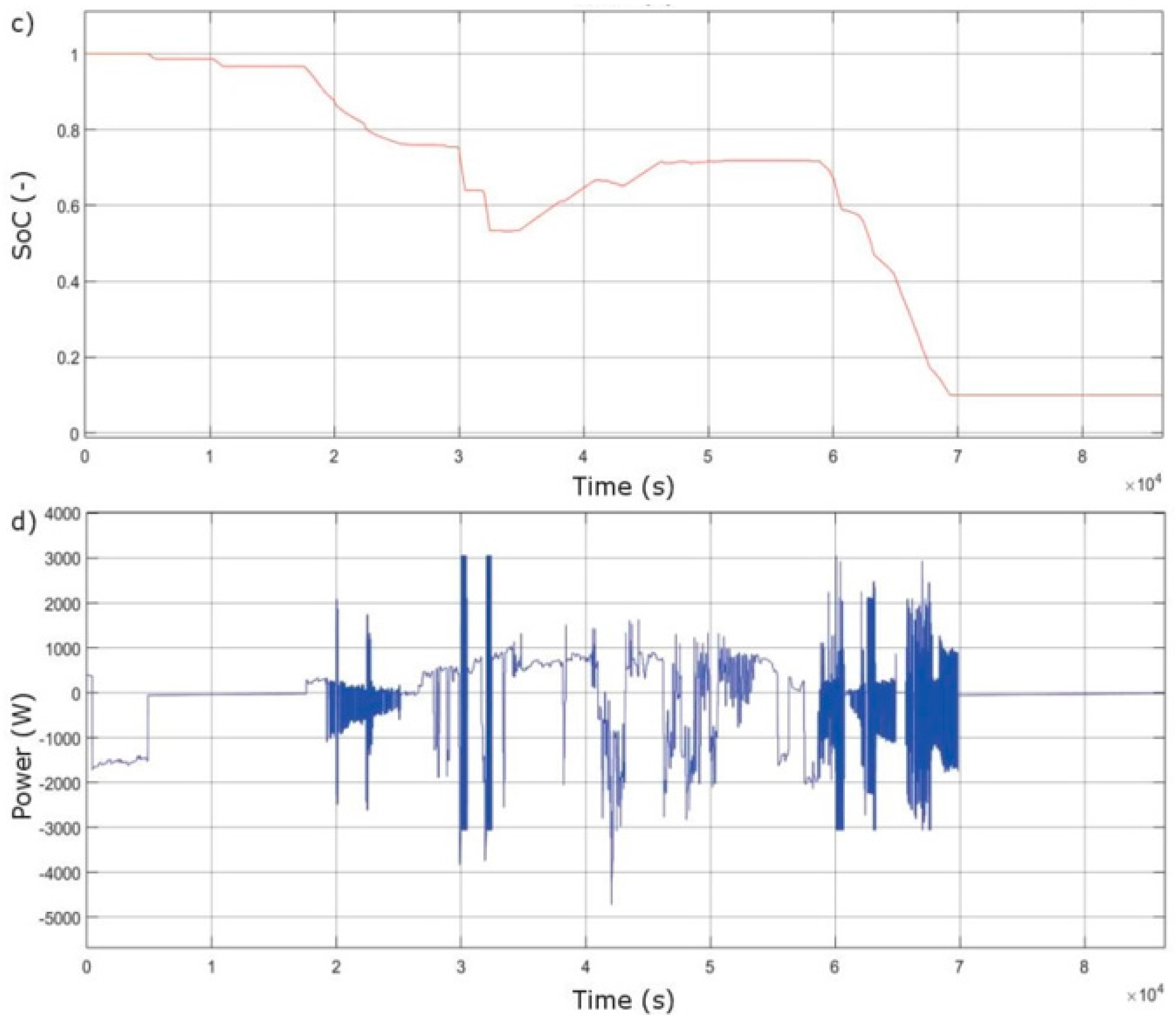
To this aim, Figure 13 shows the simulation results, as exemplified for 30% irradiation, in the case of flywheel absence. It is possible to observe, with respect to Figure 12, that the battery discharge profile is more fluctuating.

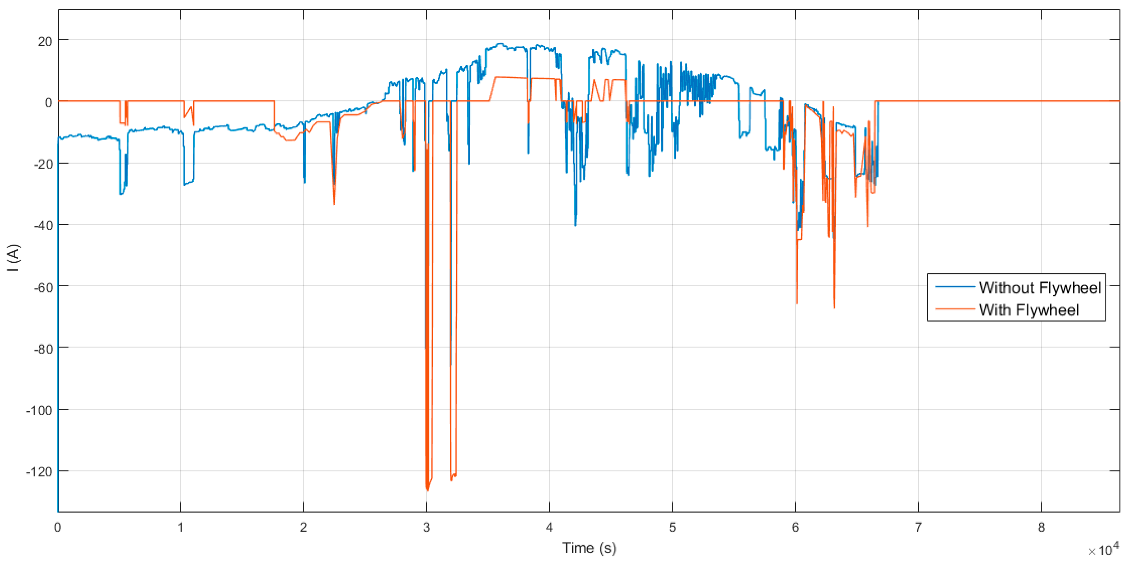
This is even clearer by comparing the profiles, with and without flywheel, of the current signal entering into the battery pack. In Figure 14, it is easy to notice that in case of flywheel absence, the battery current is characterized by a profile with higher oscillation, lacking the peak shaving function.

To quantify the oscillation reduction provided by the flywheel introduction towards both battery and grid, a comparison on fluctuation indexes between the operation with and without flywheel is done.

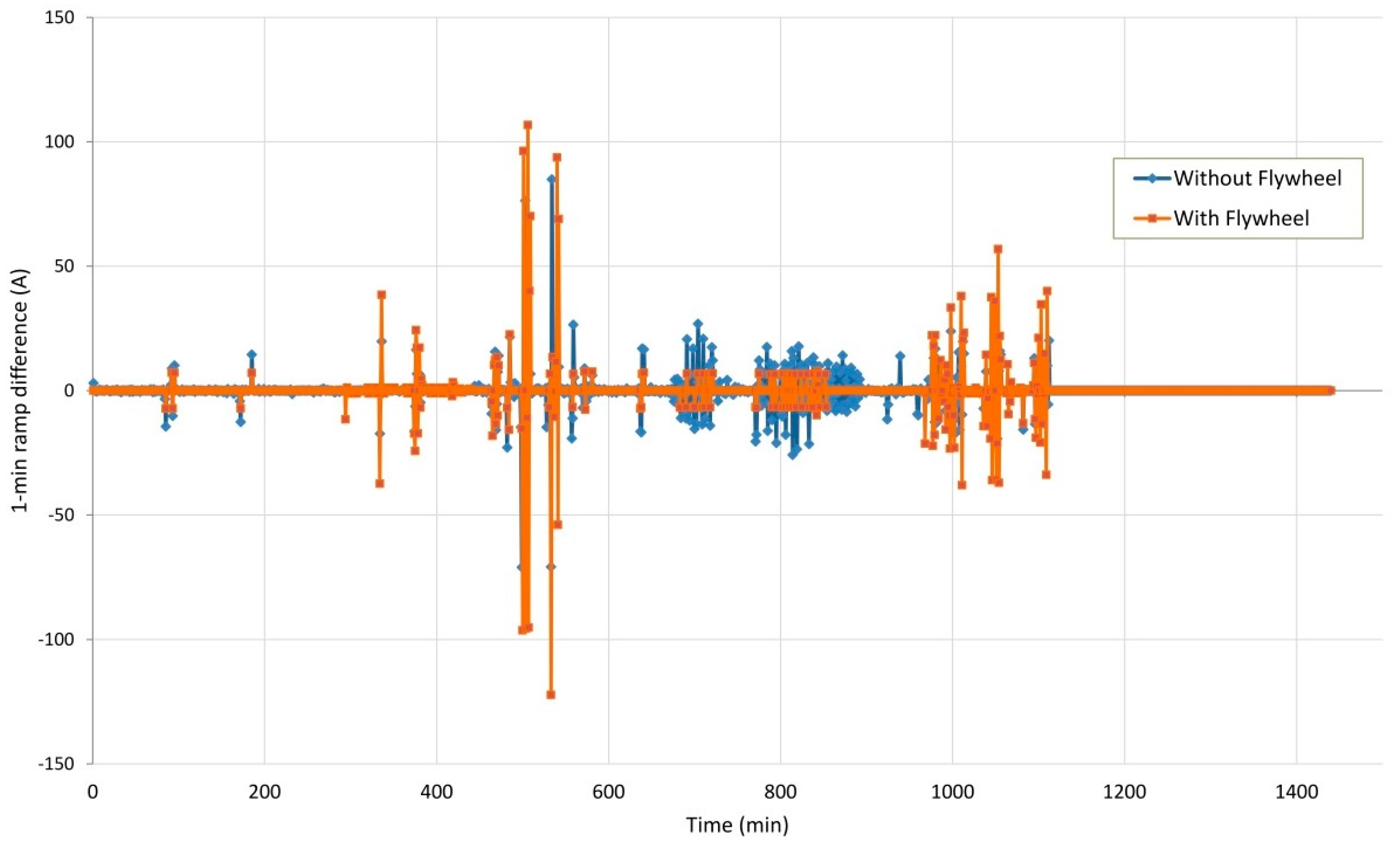
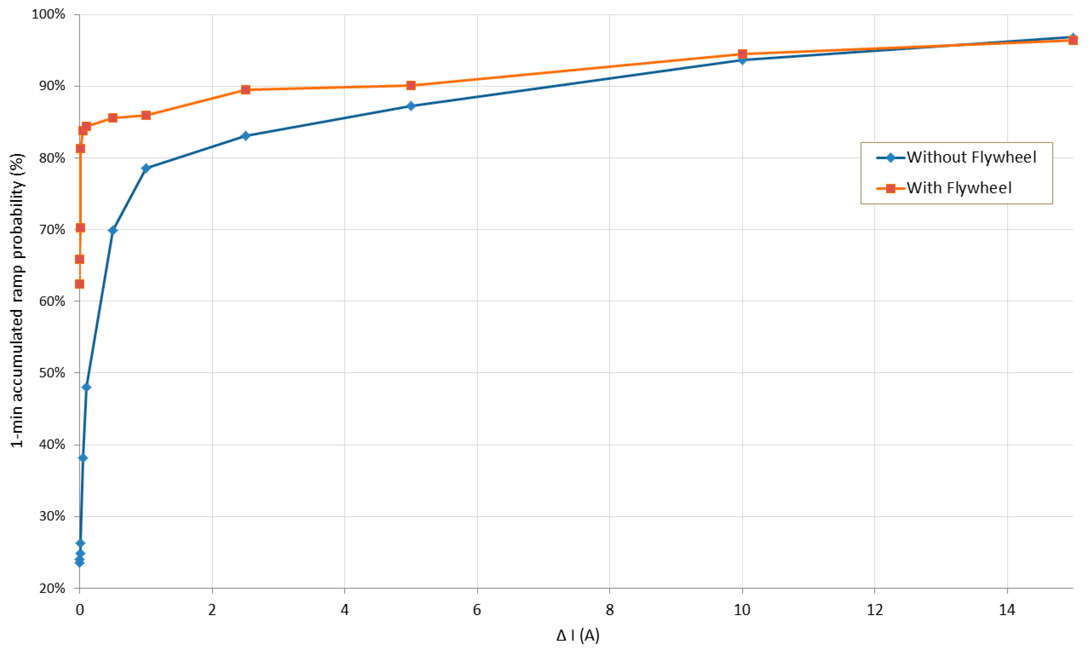
Firstly, the battery current profile was studied considering as example a 30% irradiation day. Figure 15 and Figure 16 represent the 1-min differential form of fluctuation and the accumulated ramp probability function respectively. Specifically to improve the results readability, Figure 16 provides a zoom of the 1-min ramp probability up to 15 A, anyway covering the 96% of samples. With reference to this figure, it is noted that for 90% of the day the oscillation, evaluated with a 1 min time step, is below 3 amps while this value rises to 7 A in the absence of the flywheel.

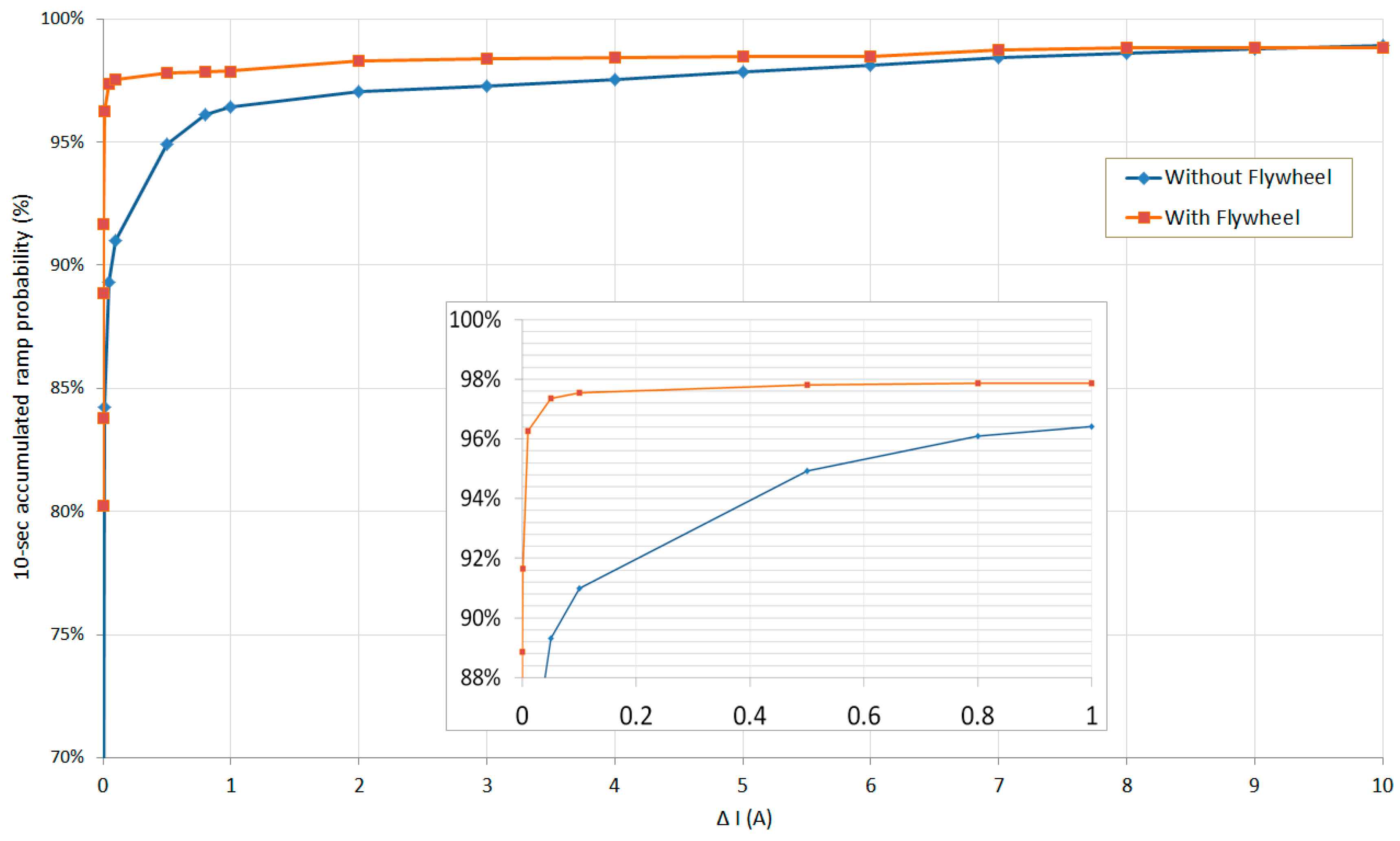
For completeness, Figure 17 and Figure 18 provide the ramp difference and the accumulated ramp probability for a 10 s time step. In confirmation of what already said, also in this case, it’s clear the advantage due to the flywheel introduction in a MG. In fact, in Figure 17a sensible reduction of the current can be identified. Moreover, in Figure 18 it is noted that for 96% of the day, the current oscillation is less than 0.01 A but it increases to 0.8 A without a H-ESS.

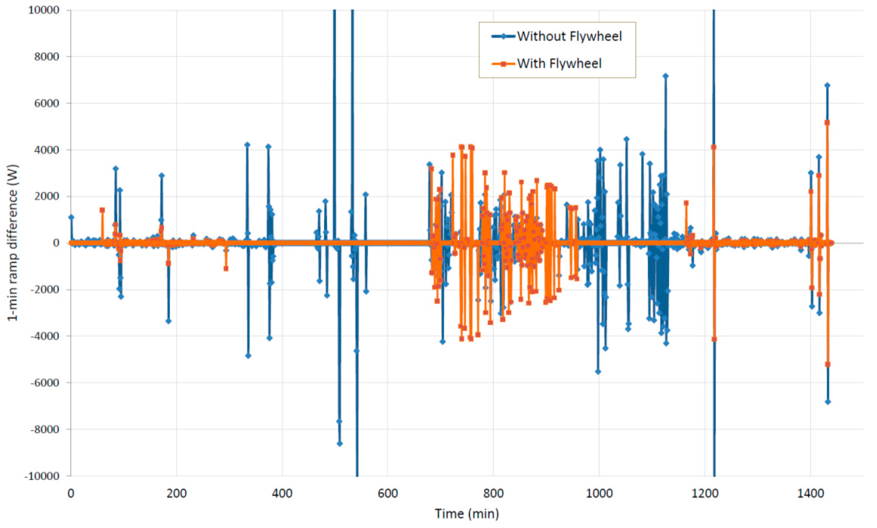
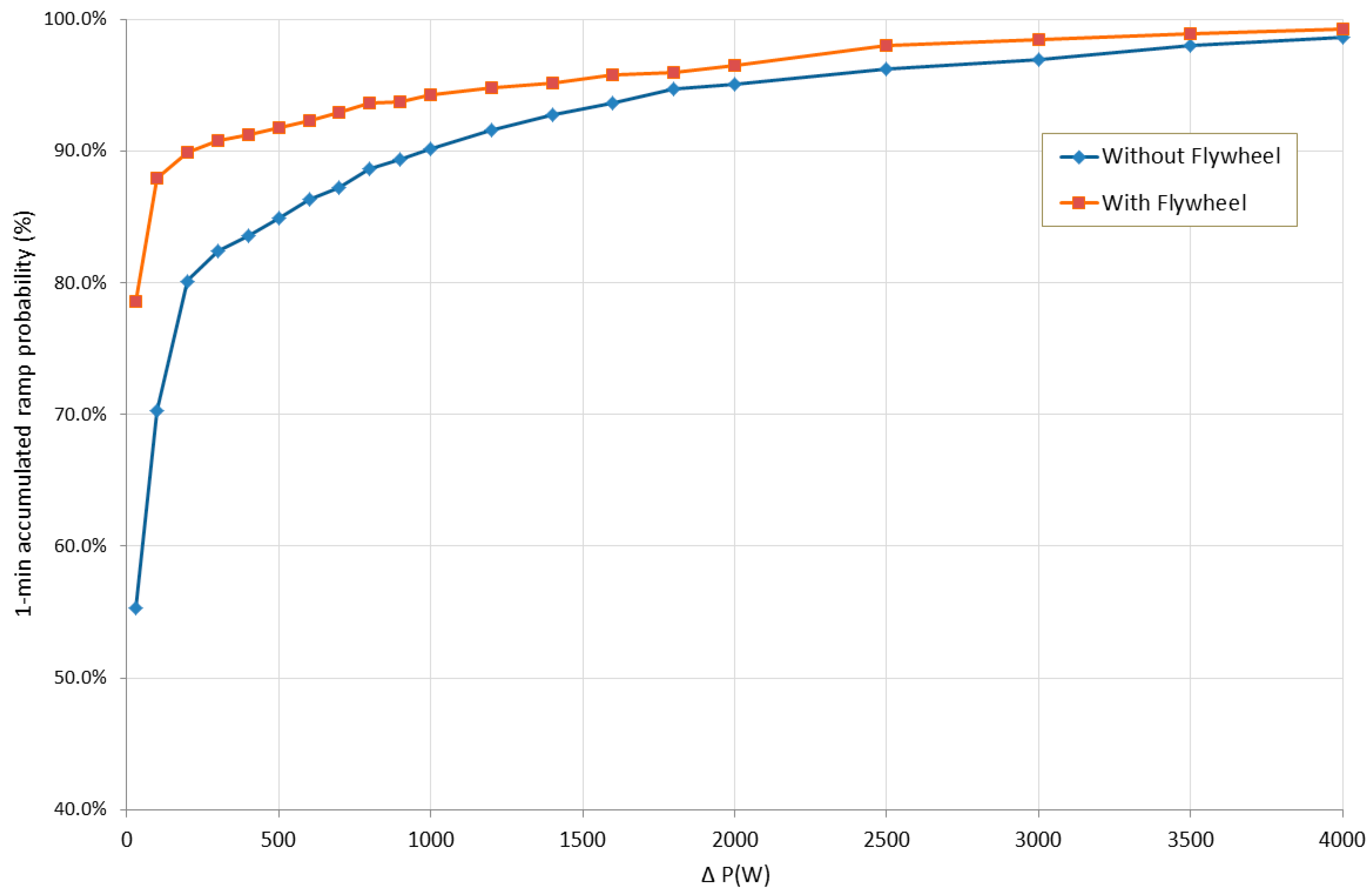
Relevant benefits were detected also in reference to the power exchanged with grid. Power variation was evaluated for both 1 min and 10 s time steps, on the basis of the power profile simulated for a 50% irradiation. This condition is needed to have a profile characterized by power sent to the grid comparable to power from the grid. Specifically, Figure 19 and Figure 20 show the ramp difference and the accumulated ramp probability of power variation for a 1 min time step. It is clear as in the H-ESS case the power fluctuations are reduced leading to, in the cumulated distribution, 90% of samples with amplitude at maximum of 200 W instead of 1000 W (without flywheel).

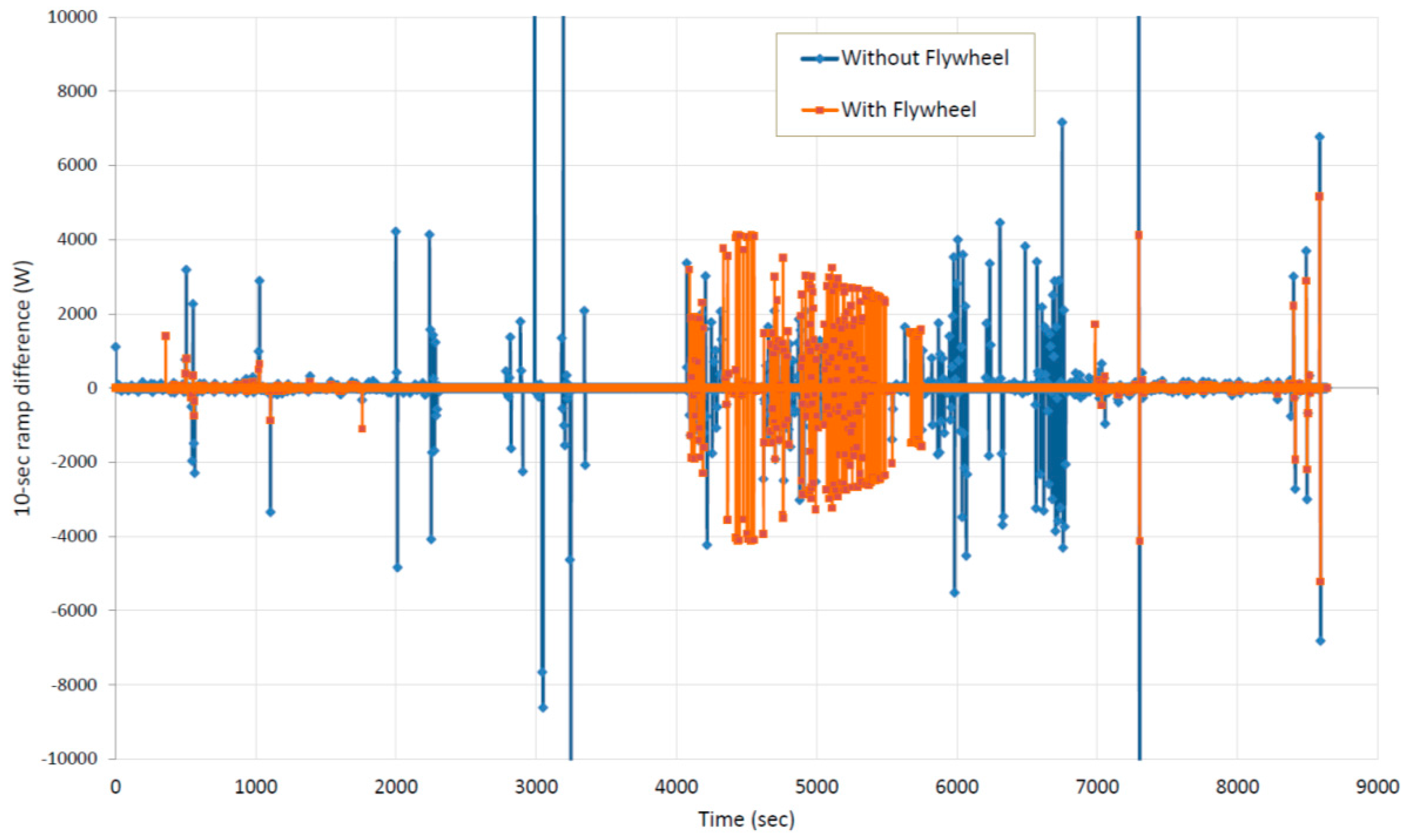
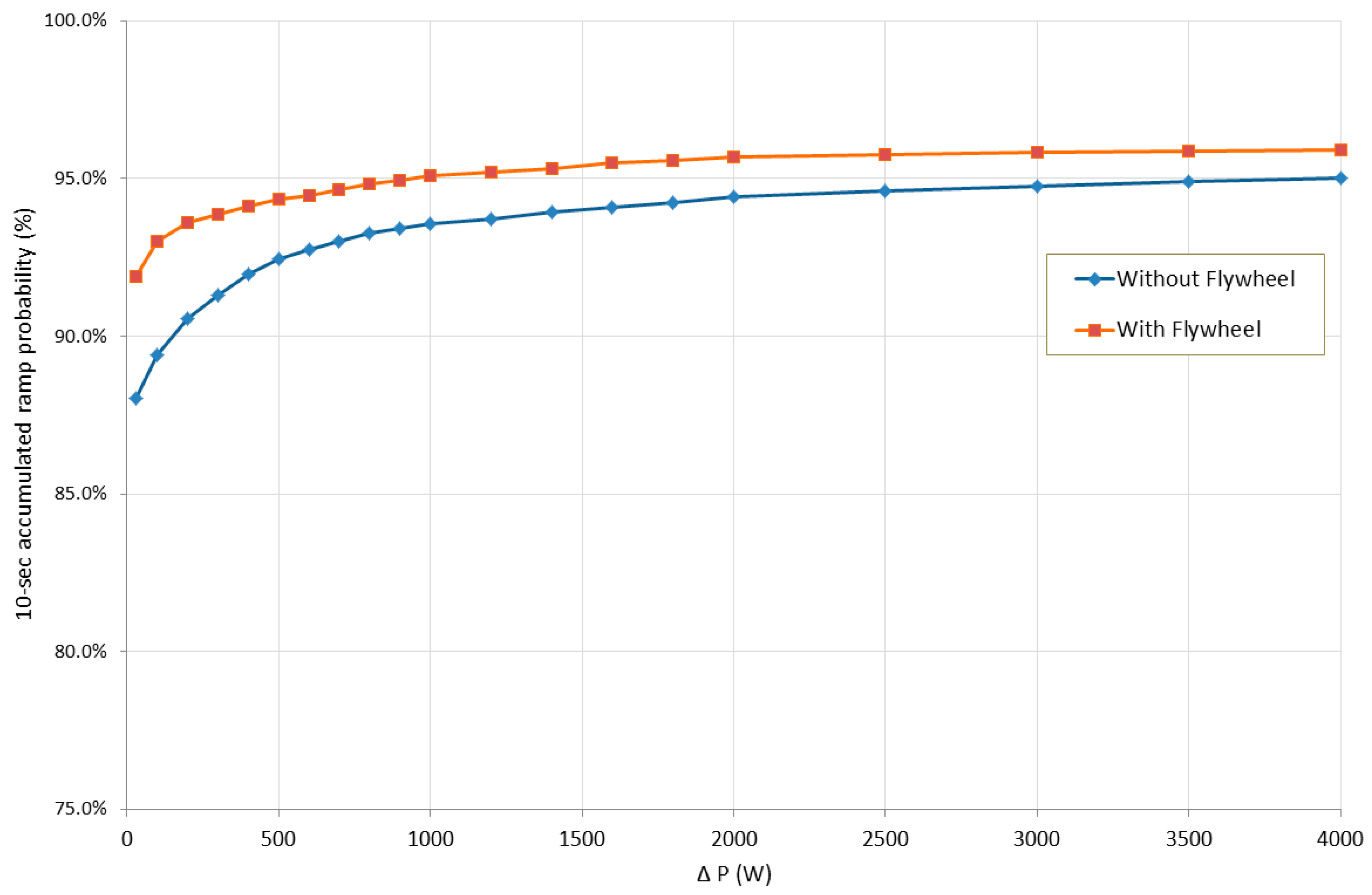
Figure 21 and Figure 22 present the same analysis with 10 s time step. Referring to the accumulated ramp probability plot, the hybridization allows to reduce, at 95% of samples, the power amplitude from 4000 W to 1000 W.

Concluding, as it can be seen from the profiles shown, flywheel works in a collaborative way with battery, shaving the load fluctuations towards both battery and grid, consequently with benefits in terms of battery durability and grid safety and stability.

6. Conclusions

This paper provides a dynamic analysis of a hybrid flywheel-battery energy storage system coupled to a photovoltaic generation plant and a residential load. Thanks to the development of a MG dynamic model, the instantaneous behaviour of each component and the mutual interconnections between the singular components are characterized. This analysis takes also into account of the effect of components sizing, power flow control strategy and weather conditions. This hybridization has allowed to merge the positive features of base storage technologies extending, in this way, their application ranges. Specifically, the flywheel peak-shaving function, typically usable in power quality applications, finds in H-ESS an implementation with a useful effect in energy storage applications. Enhanced performances of the overall H-ESS, as briefly listed below, are provided with respect to the case of battery storage systems:

- Enhanced duration. The issue related to the battery cycling is mitigated by the peak-shaving function of the flywheel as demonstrated in terms of the oscillation reduction of the battery load profile. In fact, with regard to the simulation conditions, it is quantified that this oscillation, valued with a 1 min time step, is maintained for 90% of the day below 3 A, while this value rises to 7 A in the case of only installed battery. Evaluating with a reduced time step of 10 s, for 96% of the day, the battery suffers extremely low current oscillation (0.01 A) that rises to 1 A in the absence of the flywheel. In [35] the effect of oscillation reduction on battery lifetime is quantified by applying rainflow algorithm.

- Improvement of the quality of the power exchanged with grid. Specifically, considering 1 min and 10 s time steps, the power fluctuations are reduced respectively five times, during the 90% of the day, and four times for 95% of daily samples.