A Steady-State Analysis Method for Modular Multilevel Converters Connected to Permanent Magnet Synchronous Generator-Based Wind Energy Conversion Systems

Abstract

Modular multilevel converters (MMCs) have shown great potential in the area of multi-megawatt wind energy conversion system (WECS) based on permanent magnet synchronous generators (PMSGs). However, the studies in this area are few, and most of them refer to the MMC used in high-voltage direct current (HVDC) systems, and hence the characteristics of the PMSG are not considered. This paper proposes a steady-state analysis method for MMCs connected to a PMSG-based WECS. In the proposed method, only the wind speed (operating condition) is required as input, and all the electrical quantities in the MMC, including the amplitudes, phase angles and their harmonics, can be calculated step by step. The analysis method is built on the proposed d-q frame mathematical model. Interactions of electrical quantities between the MMC and PMSG are comprehensively considered. Moreover, a new way to calculate the average switching functions are adopted in order to improve the accuracy of the analysis method. Applications of the proposed method are also presented, which includes the characteristic analysis of capacitor voltage ripples and the capacitor sizing. Finally, the accuracy of the method and the correctness of the analysis are verified by simulations and experiments.

1. Introduction

Wind energy, as one of the fastest growing renewable energy sources, is gradually becoming mainstream and competitive with conventional energy sources [1,2,3,4]. The installed capacity of wind energy has increased from 6100 MW in 1996 to 432,883 MW by 2015 [2]. The continuous growth in demand for wind energy promotes the development of larger wind turbines, because the large turbines can capture more wind power with lower installation and maintenance costs, compared to the group of small turbines [5]. The size and capacity of commercial wind turbines have exponentially increased over the past 30 years, and has currently reached the level of 10MWs [2,5].

In multi-megawatt wind energy conversion systems (WECS), permanent magnet synchronous generators (PMSGs) with full-scale power converters have been widely adopted, due to their salient features such as high-power density, no need of excitation, and high efficiency. However, as the power capacity of wind turbines has increased up to 10 MW, the traditional two- and three-level converters require a large amount of series or parallel connected power devices in order to achieve the required power, which reduces the reliability of WECS. Moreover, the traditional converters are not suitable for medium-voltage (3–33 kV) WECS, which is becoming popular for turbine power ratings greater than 3.0 MW [6,7]. These drawbacks lead to the studies of new full-scale power converters.

The modular multilevel converter (MMC), which became the most common type of voltage-source converter used in the high-voltage direct current (HVDC) applications, is also a suitable converter for PMSG-based WECS. In [8,9], MMC was used for medium-voltage motor drives, which opened up the study of MMC applied to variable-speed machines. The application of MMCs in PMSG-based WECS was first studied in [10]. That paper concluded that MMC should be considered a suitable option for transformerless 10 MW PMSG-based WECS, and performs well in the full system. In [11], the authors proposed an improved online fault identification scheme for the MMC applied to WECS, which avoided the use of extra sensors by only using the already available variables in detection, and therefore the maintenance cost of the distant offshore wind farms can be reduced. In [12], the complete control scheme of MMC applied to the PMSG-based WECS was proposed. Low voltage ride-through problems and capacitor voltage ripple problems were also studied in that paper. In addition, the increasing interest in all-dc wind farms, in recent years, will also enlarge the application of MMC in WECS [13,14,15].

Steady-state analysis can be used for component sizing and assessment of the impact of different parameters on the MMC performance. However, there is no reference available for the steady-state analysis of the MMC connected to a PMSG. Most of the analysis methods and techniques are referred to the MMC used in HVDC or motor drives. The MMC connected to the PMSG-based WECS is a complicated system. The electrical quantities in MMC and PMSG are coupled with each other. This means that the MMC and PMSG cannot be analyzed separately, and the characteristics of PMSG must be considered while analyzing the MMC. Moreover, different from the MMC used in HVDC, the output voltage of the MMC connected to PMSG is variable according to operating conditions (wind speed). Therefore, this paper proposes a steady-state analysis method for MMC connected to the PMSG-based WECS. There are previous papers, which draws the interests on the steady-state analysis of MMC used in HVDC. Paper [16] documented the interactions between arm currents and capacitor voltages, and derived the equations of circulating current and capacitor voltage harmonics. A study conducted in [17] proposed a circular interaction among the electrical quantities in an MMC, and deduced the formula of the unknown circulating current based on that circular interaction. An accurate capacitor voltage ripple estimation method was proposed in paper [18], where common-mode voltage injections and intentionally imposed circulating currents were taken into consideration. In [19], authors proposed a closed-loop analysis method and derived the harmonics of electrical quantities in MMC in detail. In comparison to the previous papers, the steady-state analysis method proposed in this paper has the following novel features:

• The analysis method is built on the proposed d-q frame mathematical model of MMC connected to a PMSG. Interactions of electrical quantities between the MMC and PMSG are comprehensively considered. In the d-q frame mathematical model, the time-varying quantities are transformed into constant quantities, which therefore simplifies the derivation. Due to this, the equivalent resistances in the MMC arms can be considered, and the algebraic solution of non-linear equations can be obtained to calculate the unknowns in the average switching functions.
• Only the wind speed (operating condition) is required as input, and all the electrical quantities in MMC, including the amplitudes, phase angles and their harmonics, can be calculated step by step, when the parameters, such as the capacitance and inductance in the MMC and the flux linkage in the PMSG, are set down.
• In order to improve the accuracy of the analysis, a new way to calculate the average switching functions in the mathematic model are adopted. In addition, the calculation results are obtainable at one stroke and no need for iteration. Therefore, the accuracy of analysis can be improved without sacrificing a lot calculation speed.
• Capacitor voltage ripple is one of the key problems in the MMC connected to variable-speed machines; this problem is further analyzed based on the proposed analysis method. The analysis results show that the MMC connected to PMSG has different characteristics from the MMC used for motor drives. A capacitor sizing method for MMC connected to PMSG is also proposed in this paper.

The rest of the paper is organized as follows: Section 2 builds the d-q frame mathematical model of a MMC connected to a PMSG. The equations of electrical quantities in the MMC are derived in Section 3. Section 4 presents the new method to calculate the average switching functions, and then provides the flow chart of the proposed steady-state analysis method. In Section 5, applications of the proposed method are presented, which includes the characteristic analysis of capacitor voltage ripples and the capacitor sizing. In Section 6 and Section 7, the simulations and experiments are carried out to validate the accuracy of the proposed method. Section 8 provides the conclusions of this work.

2. Modelling of MMC Connected to the PMSG-Based WECS

2.1. MMC Connected to the PMSG-Based WECS

Figure 1 shows the typical structure of a MMC connected to the PMSG-based WECS. At first, the wind energy is converted into mechanical power by blades. Then, the mechanical power is converted into electrical power via PMSG. Finally, the MMC rectifies the ac power into dc power, and transfers the electrical power from the PMSG to the dc bus.

During the wind energy conversion process, there is a strong coupling relationship between PMSG and MMC, which is shown in Figure 1 by the blue dashed lines. The wind energy ($P_{wind}$) determines the input mechanical power ($P_m$), which then affects mechanical torque ($T_m$) and rotor speed (${\omega }_m$). The rotor speed influences the output voltage of PMSG ($u_a$), which determines the phase current ($i_a$). The phase current is part of the arm current ($i_{arm}$) in MMC, and it affects the capacitor current ($i_{cap}$) and voltage ($u_{cap}$). The capacitor voltage determines the output voltage of sub-module ($u_{sub}$), which afterwards affects the phase currents by influencing the electromotive force (EMF) of MMC (not shown in Figure 1). Finally, the phase current in return determines the electromagnetic torque ($T_e$), and then the electromagnetic torque in return affects the rotor speed.

Because of this strong coupling relationship, the analysis of MMC connected to the PMSG-based WECS becomes complicated. Hence, in this section, the basic configuration of MMC is described first, and then the mathematical model of MMC connected to the PMSG-based WECS is built in the d-q frame. The established d-q frame mathematical model is the basement of the proposed steady-state analysis method, and it can also further help to understand the coupling relationship.

2.2. Basic Configuration of MMC

As shown in Figure 1, the three ac terminals of MMC are connected to the positive and negative dc bus bars through three upper and lower arms. There, $i_{arm.j.up}$ and $i_{arm.j.dn}$ (j = a, b, c, similarly hereinafter) denote the arm currents of upper and lower arms, respectively. $u_{cap}$ and $i_{cap}$ are capacitor voltage and current. C denotes the capacitor in submodules. $u_{sub}$ and $i_{sub}$ are submodule current and voltage. $L_{arm}$ is the arm inductor. $I_{dc}$ and $U_{dc}$ denote the dc-side current and voltage.

Different from the MMC connected to the power grid, the frequency in the MMC connected to PSMG varies with the mechanical angular speed of PMSG rotor and is also affected by the number of pole-pairs in the generator, which can be expressed as:

$$\omega ={\omega }_r=p{\omega }_m$$

(1)

where, $\omega$ is the angular speed of MMC; ${\omega }_r$ and ${\omega }_m$ denote the electrical and mechanical angular speed of the rotor in PMSG; $p$ is the number of pole-pairs.

Therefore, it is more convenient to take the d-axis of PMSG rotor flux as the datum line. In other words, the MMC model is built in the coordinate system of PMSG, and the phase angle of the ac-side voltage of MMC is no longer zero, as it used to be.

Taking phase A for example, the ac-side voltage of MMC can be defined as:

$$u_a(t)=U_s\cos (\omega t+\varphi )$$

(2)

where, $U_s$ and $\varphi$ are the amplitude and the phase angle of the output voltage.

According to the previous papers [17,18], the arm current of MMC is consisted of the dc component, phase current component and circulating current component, which can be expressed as:

$$i_{arm.a.up}(t)=\frac{I_{dc}}{3}-\frac{i_a(t)}{2}+i_{cir.a}(t)$$

(3)

$$i_{arm.a.dn}(t)=\frac{I_{dc}}{3}+\frac{i_a(t)}{2}+i_{cir.a}(t)$$

(4)

where:

$$i_a(t)=I_s\cos (\omega t+\phi )$$

(5)

$$i_{cir.a}(t)=I_{cir}\cos (2\omega t+{\theta }_{cir})$$

(6)

$I_s$ and $\phi$ are the amplitude and the phase angle of phase current. $I_{cir}$ and ${\theta }_{cir}$ denote the amplitude and the phase angle of 2nd harmonic circulating current.

It should be noted that although there are 4th and higher even-order harmonics in the circulating current, they are usually controlled to be small enough to be neglected [20]. Hence, only 2nd harmonics are considered in this paper.

The upper and lower arm voltages of MMC are defined as the sum of sub-module voltages $u_{sub}$ in their respective arm:

$$u_{arm.a.up}(t)={\displaystyle \sum _{i=1}^N{u}_{sub.a.up.i}(t)}$$

(7)

$$u_{arm.a.dn}(t)={\displaystyle \sum _{i=1}^N{u}_{sub.a.dn.i}(t)}$$

(8)

where, N is the number of submodules in one arm.

From Kirchhoff’s law and Equations (2)–(8), the following two equations can be obtained:

$$\frac{U_{dc}}{2}-u_a(t)=u_{arm.a.up}(t)+R_{eq}{i}_{arm.a.up}(t)+L_{arm}\frac{d{i}_{arm.a.up}(t)}{dt}$$

(9)

$$\frac{U_{dc}}{2}+u_a(t)=u_{arm.a.dn}(t)+R_{eq}{i}_{arm.a.dn}(t)+L_{arm}\frac{d{i}_{arm.a.dn}(t)}{dt}$$

(10)

Then, Equations (11) and (12) can be derived based on Equations (9) and (10):

$$u_a(t)=e_{MMC.a}(t)+\frac{R_{eq}}{2}{i}_a(t)+\frac{L_{arm}}{2}\frac{d{i}_a(t)}{dt}$$

(11)

$$\frac{U_{dc}}{2}-u_{com.a}(t)=\frac{R_{eq}{I}_{dc}}{3}+R_{eq}{i}_{cir.a}(t)+L_{arm}\frac{d{i}_{cir.a}(t)}{dt}$$

(12)

where, the EMF $e_{MMC.a}$ and the common-mode voltage $u_{com.a}$ are defined as:

$$e_{MMC.a}(t)=\frac{u_{arm.a.dn}(t)-u_{arm.a.up}(t)}{2}$$

(13)

$$u_{com.a}(t)=\frac{u_{arm.a.up}(t)+u_{arm.a.dn}(t)}{2}$$

(14)

The EMF consists of the fundamental component and the odd-order harmonics. However, the odd-order harmonics are usually less than a hundredth of the fundamental component, and hence can be ignored. The EMF of phase A can be defined as:

$$e_{MMC.a}(t)=E_{MMC}\cos (\omega t+\alpha )$$

(15)

where, $E_{MMC}$ and $\alpha$ are the amplitude and the phase angle of EMF.

Equation (11) reflects the external characteristic of MMC, and expresses the relationship between the output voltage and EMF. Equation (12) reflects the internal characteristic of MMC, and describes the relationship between the common-mode voltage and circulating current.

2.3. Modelling of MMC Connected to the PMSG-Based WECS

It is assumed that in the steady state, the time delay of phase B and C are T/3 and 2T/3 respectively with phase A as the reference phase, where T is the fundamental period of the electrical quantities. It should be noted that the 2nd harmonic quantities are negative sequence.

Using the standard model, the voltage equations of PMSG can be expressed in the d-q frame as follows [21,22]:

$$u_d(t)=-R_s{i}_d(t)+\omega L_q{i}_q(t)-L_d\frac{d{i}_d(t)}{dt}$$

(16)

$$u_q(t)=-R_s{i}_q(t)-\omega L_d{i}_d(t)+\omega {\lambda }_m-L_q\frac{d{i}_q(t)}{dt}$$

(17)

where, ${\lambda }_m$ represents the maximum flux produced by the permanent magnet; $L_d$ and $L_q$ are the d-axis and q-axis synchronous inductance respectively; $R_s$ is the stator resistance; $u_d$ and $u_q$ are the d-axis and q-axis output voltage of PMSG.

In order to obtain the MMC mathematical model in the d-q frame, the Equations (11) and (12) should firstly be rewritten into three-phase form:

$$\left[\begin{array}{c}{u}_a(t)\\ u_b(t)\\ u_c(t)\end{array}\right]=\left[\begin{array}{c}{e}_{MMC.a}(t)\\ e_{MMC.b}(t)\\ e_{MMC.c}(t)\end{array}\right]+\frac{R_{eq}}{2}\left[\begin{array}{c}{i}_a(t)\\ i_b(t)\\ i_c(t)\end{array}\right]+\frac{L_{arm}}{2}\frac{d}{dt}\left[\begin{array}{c}{i}_a(t)\\ i_b(t)\\ i_c(t)\end{array}\right]$$

(18)

$$\frac{U_{dc}}{2}-\left[\begin{array}{c}{u}_{com.a}(t)\\ u_{com.b}(t)\\ u_{com.c}(t)\end{array}\right]=\frac{R_{eq}{I}_{dc}}{3}+R_{eq}\left[\begin{array}{c}{i}_{cir.a}(t)\\ i_{cir.b}(t)\\ i_{cir.c}(t)\end{array}\right]+L_{arm}\frac{d}{dt}\left[\begin{array}{c}{i}_{cir.a}(t)\\ i_{cir.b}(t)\\ i_{cir.c}(t)\end{array}\right]$$

(19)

Based on the superposition theorem, the 2nd harmonic current is generated by the 2nd harmonic voltage [16]. Equation (19) can then be deduced as:

$$-\left[\begin{array}{c}{u}_{com.2\omega .a}(t)\\ u_{com.2\omega .b}(t)\\ u_{com.2\omega .c}(t)\end{array}\right]=R_{eq}\left[\begin{array}{c}{i}_{cir.a}(t)\\ i_{cir.b}(t)\\ i_{cir.c}(t)\end{array}\right]+L_{arm}\frac{d}{dt}\left[\begin{array}{c}{i}_{cir.a}(t)\\ i_{cir.b}(t)\\ i_{cir.c}(t)\end{array}\right]$$

(20)

where, $u_{com.2\omega .j}$ denotes the 2nd harmonic in the common-mode voltage.

By applying the d-q transformations to Equations (18) and (20), the following equations can be obtained:

$$\left[\begin{array}{c}{u}_d(t)\\ u_q(t)\end{array}\right]=T(\omega )\left[\begin{array}{c}{u}_a(t)\\ u_b(t)\\ u_c(t)\end{array}\right]=\left[\begin{array}{c}{e}_{MMC.d}(t)\\ e_{MMC.q}(t)\end{array}\right]+\frac{R_{eq}}{2}\left[\begin{array}{c}{i}_d(t)\\ i_q(t)\end{array}\right]+\frac{L_{arm}}{2}\left[\begin{array}{c}-\omega i_q(t)\\ \omega i_d(t)\end{array}\right]+\frac{L_{arm}}{2}\frac{d}{dt}\left[\begin{array}{c}{i}_d(t)\\ i_q(t)\end{array}\right]$$

(21)

$$\left[\begin{array}{c}{u}_{com.d}(t)\\ u_{com.q}(t)\end{array}\right]=T(2\omega )\left[\begin{array}{c}{u}_{com.2\omega .a}(t)\\ u_{com.2\omega .c}(t)\\ u_{com.2\omega .b}(t)\end{array}\right]=-R_{eq}\left[\begin{array}{c}{i}_{cir.d}(t)\\ i_{cir.q}(t)\end{array}\right]-L_{arm}\left[\begin{array}{c}-2\omega i_{cir.q}(t)\\ 2\omega i_{cir.d}(t)\end{array}\right]-L_{arm}\frac{d}{dt}\left[\begin{array}{c}{i}_{cir.d}(t)\\ i_{cir.q}(t)\end{array}\right]$$

(22)

where, $T(\theta )$ ($\theta$ = $\omega$, $2\omega$) is the d-q transformation matrix, and is shown in Equation (23):

$$T(\theta )=\frac{2}{3}\left[\begin{array}{c}\begin{array}{ccc}\cos (\theta )& \cos (\theta -\frac{2}{3}\mathsf{\pi })& \cos (\theta +\frac{2}{3}\mathsf{\pi })\end{array}\\ \begin{array}{ccc}-\sin (\theta )& -\sin (\theta -\frac{2}{3}\mathsf{\pi })& -\sin (\theta +\frac{2}{3}\mathsf{\pi })\end{array}\end{array}\right]$$

(23)

From Equations (16), (17), (21) and (22), the d-q frame mathematical model of MMC connected to the PMSG-based WECS can be expressed as:

$$\omega L_q{i}_q(t)-R_s{i}_d(t)-L_d\frac{d{i}_d(t)}{dt}=e_{MMC.d}(t)+\frac{R_{eq}}{2}{i}_d(t)-\frac{L_{arm}}{2}\omega i_q(t)+\frac{L_{arm}}{2}\frac{d{i}_d(t)}{dt}$$

(24)

$$\omega {\lambda }_m-\omega L_d{i}_d(t)-R_s{i}_q(t)-L_q\frac{d{i}_q(t)}{dt}=e_{MMC.q}(t)+\frac{R_{eq}}{2}{i}_q(t)+\frac{L_{arm}}{2}\omega i_d(t)+\frac{L_{arm}}{2}\frac{d{i}_q(t)}{dt}$$

(25)

$$u_{com.d}(t)=-R_{eq}{i}_{cir.d}(t)+2\omega L_{arm}{i}_{cir.q}(t)-L_{arm}\frac{d{i}_{cir.d}(t)}{dt}$$

(26)

$$u_{com.q}(t)=-R_{eq}{i}_{cir.q}(t)-2\omega L_{arm}{i}_{cir.d}(t)-L_{arm}\frac{d{i}_{cir.q}(t)}{dt}$$

(27)

Based on the mathematical model, the following equivalent circuit can be obtained. As shown in Figure 2, the upper two circuits are the d-axis equivalent circuits, which are built based on Equations (24) and (26). The lower two circuits are q-axis equivalent circuits, which are built based on Equations (25) and (27). In addition, Equations (24) and (25) describe the relationship between PMSG and MMC. Equations (26) and (27) represent the relationship between 2nd common-mode voltages and circulating currents in MMC.

It should be noted that the four equations are not independent. As is shown by the blue dashed line in Figure 2, the four equivalent circuits (or equations) are coupled with each other by the capacitors installed in MMC. This coupling relationship can be described as follows. The phase currents ($i_d$, $i_q$) and circulating currents ($i_{cir.d}$, $i_{cir.q}$) make up the ac components of arm currents. Then the arm currents will charge and discharge the capacitors, which causes the capacitor voltage ripple. The voltage ripple mainly contains fundamental frequency, 2nd order and 3rd order components, and will be delivered to the arm voltages.

From Equations (13) and (14), the EMF and common-mode voltage can be calculated based on the arm voltages. Consequently, on the one hand, the odd-components of arm voltages will cause changes in the phase angle and amplitude of EMF, and then change in EMF, in return, influence the phase currents. On the other hand, the 2nd components of arm voltages make up the 2nd components of common-mode voltages, and become the voltage sources of 2nd circulating currents. The coupling relationship described in Figure 2 is the electrical part in the coupling relationship described in Figure 1. There are mainly two benefits to build the mathematical model in the d-q frame for MMC connected to the PMSG-based WECS:

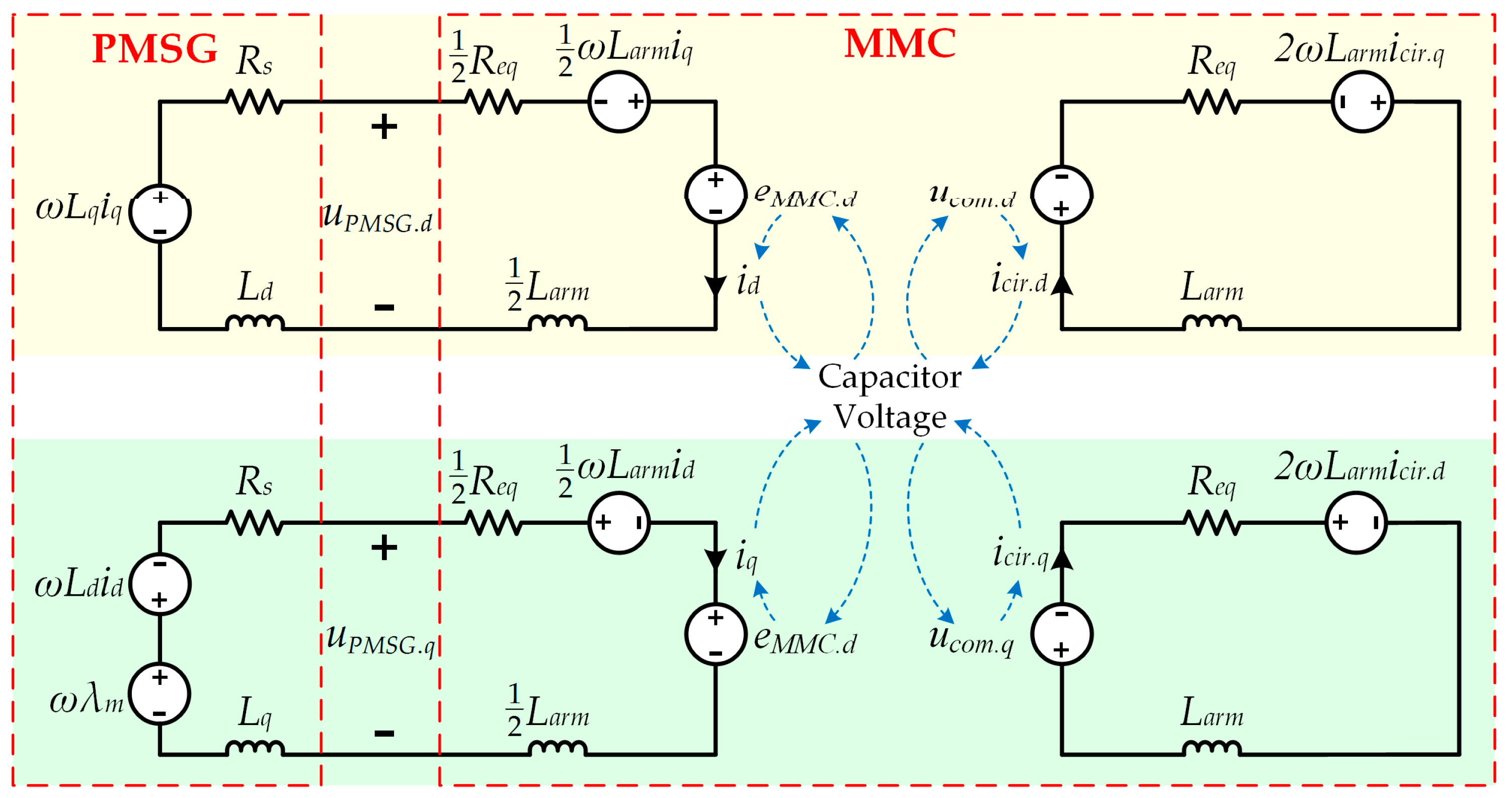
• Modelling MMC in the d-q frame facilitates the establishment of associations between the electrical quantities in PMSG and the electrical quantities in MMC, because the mathematical model of PMSG is built in the d-q frame, and the d-axis and q-axis synchronous inductances are not equal for the salient-pole PMSG.
• In the d-q frame mathematical model, the time-varying quantities are transformed into constant quantities, which therefore can simplify the derivation. Due to this, the equivalent resistances in the MMC arms can be considered in the analysis, and the algebraic solution of non-linear equations can be obtained to calculate the amplitudes and phase angles of average switching functions.

3. Calculation of the Electrical Quantities in MMC

3.1. A More Accurate Method to Calculate the Average Switching Function

IGBT gate signals, which control the on/off state of the IGBTs, directly determine the operation of MMC. In the mathematical model of MMC, the IGBT gate signals are described as the switching function, which can be expressed as follows:

$$S_i(t)=\{\begin{array}{c}1, \mathrm{when} S_1 \mathrm{is} \mathrm{on} \mathrm{and} S_2 \mathrm{is} \mathrm{off}\\ 0, \mathrm{when} S_1 \mathrm{is} \mathrm{off} \mathrm{and} S_2 \mathrm{is} \mathrm{on}\end{array}$$

(28)

where, S_i(t) denotes the switching function. S₁ and S₂ is the upper and lower IGBT in each sub-module respectively, which is shown in Figure 1.

The mathematical expression of the switching function in Equation (28) is a discrete function and difficult to be obtained, therefore the average switching function is normally adopted in the mathematical model of MMC [17]. Taking phase A as an example, the average switching functions of upper and lower arms can be expressed as:

$$S_{up.a}(t)=\frac{1}{2}-S_{ref.a}(t)-S_{\mathrm{add}.a}(t)$$

(29)

$$S_{dn.a}(t)=\frac{1}{2}+S_{ref.a}(t)-S_{\mathrm{add}.a}(t)$$

(30)

where, $S_{up.a}(t)$ and $S_{dn.a}(t)$ denote the average switching functions in the upper and lower arms respectively. $S_{ref.a}(t)$ is a fundamental harmonic sinusoidal function. $S_{\mathrm{add}.a}(t)$ is a 2nd harmonic sinusoidal function.

In the traditional methods, the half of the modulation index is used as the amplitude of $S_{ref.a}(t)$ [16,17]. The modulation index is defined as Equation (31). The phase angle of $S_{ref.a}(t)$ is set to be the same as the phase angle of EMF. For the 2nd harmonic components $S_{add.a}(t)$, they are ignored in the traditional methods:

$$M_e=\frac{E_{MMC}}{U_{dc}/2}$$

(31)

For the ideal condition, the capacitor voltage only contains the dc component, and can be expressed as:

$$u_{cap}(t)=\frac{U_{dc}}{N}$$

(32)

Therefore, based on Equations (7), (8) and (13), the EMF can be calculated as:

$$e_{MMC.a}(t)=\frac{u_{arm.a.dn}(t)-u_{arm.a.up}(t)}{2}=\frac{N{S}_{ap}(t)u_{cap}(t)-N{S}_{an}(t)u_{cap}(t)}{2}=E_{MMC}\cos (\omega t+\alpha )$$

(33)

The calculation result of Equation (33) equals Equation (15), which indicates that the traditional method is accurate under the ideal conditions. In fact, in addition to the dc component, the capacitor voltage also contains fundamental, 2nd and 3rd order harmonics. These harmonics are also delivered to the arm voltages, and will cause the change in the amplitude and phase angle of EMF. In other words, the calculation result of Equation (33) is not equal to Equation (15) in practice. Therefore, the traditional methods are actually inaccurate.

Consequently, a more accurate method to calculate the value of the average switching function are proposed. Figure 3 shows the overall control scheme of MMC connected to the PMSG-based WECS. The reference signal is outputted by phase current control unit, which realizes the maximum power point tracking (MPPT). The additional signal is outputted by circulating current control unit, which suppresses the circulating current. The arm voltage signal is composed of the dc component, the reference signal and the additional signal. More details of the controller are referred in paper [12], which are out of the scope of this paper.

It can be seen in Figure 3 that the IGBT gate signal is obtained by inputting the arm voltage signal into the modulation controller. In the modulation controller, since the carrier frequency is high, it makes an ignorable change to the arm voltage signal. In a word, the arm voltage signal has almost the same amplitude and phase angle as the low frequency components (dc, fundamental and 2nd) in IGBT gate signals.

Therefore, in this paper, the arm voltage signal is chosen as the value of the average switching function in the mathematical model. In other word, the reference signal in the arm voltage signal is assumed to be the fundamental component $S_{ref.a}(t)$ in the average switching function; and the additional signal in the arm voltage signal is assumed to be the 2nd harmonic component $S_{\mathrm{add}.a}(t)$ in the average switching function. The problem is that the amplitude and phase angle of the arm voltage signal are unknown. Thus, at first, the arm voltage signals are assumed to be sinusoidal functions containing unknown quantities, which are shown in Equations (34) and (35). Then, these unknown quantities will be obtained based on the coupling relationship of electrical quantities in PMSG and MMC.

Then, the average switching function can be rewritten as:

$$S_{up.a}(t)=\frac{1}{2}-\underset{\mathrm{Reference} \mathrm{Signal}}{\underbrace{M_{ref}\sin (\omega t+\beta )}}-\underset{\mathrm{Additional} \mathrm{Signal}}{\underbrace{M_{add}\sin (2\omega t+{\theta }_{add})}}$$

(34)

$$S_{dn.a}(t)=\frac{1}{2}+\underset{\mathrm{Reference} \mathrm{Signal}}{\underbrace{M_{ref}\sin (\omega t+\beta )}}-\underset{\mathrm{Additional} \mathrm{Signal}}{\underbrace{M_{add}\sin (2\omega t+{\theta }_{add})}}$$

(35)

where, $M_{ref}$ and $\beta$ are the amplitude and the phase angle of the reference signal; $M_{add}$ and ${\theta }_{add}$ are the amplitude and the phase angle of the additional signal.

In the average switching functions, although the 2nd harmonic components are smaller than the fundamental components, they are not neglected for the following two reasons:

(a)

Most of the electrical quantities in the MMC are influenced by the average switching functions, and hence adopting the more accurate average switching functions can improve the calculation accuracy.

(b)

Since the calculations are carried out in Matlab software, considering the 2nd harmonic component has only an insignificant influence on the calculation speed.

It should be noted that the four quantities ($M_{ref}$, $\beta$, $M_{add}$ and ${\theta }_{add}$) in in Equations (34) and (35) are unknown quantities. The solving method will be shown in the followings parts.

3.2. Calculation of the AC-Side Phase Current

For simplicity, the harmonics higher than 4th order are ignored in the derivation, because of their lower amplitudes compared with the fundamental components.

The ac-side phase currents in the d-q frame have the following relationship with the electromagnetic torque [5]:

$$T_e(t)=\frac{3}{2}p[{\lambda }_m{i}_q(t)-[L_d-L_q]i_d(t)i_q(t)]$$

(36)

Equation (36) means that the electromagnetic torque can be controlled by controlling phase currents. Usually, the d-axis current is controlled to be zero to remove the coupling between the d-axis and q-axis currents in the electromagnetic torque [23,24]. Hence, the phase currents can be calculated as follows:

$$i_d=0$$

(37)

$$i_q=\frac{2T_e}{3p{\lambda }_m}$$

(38)

The mechanical power extracted from wind energy is determined by the wind speed and wind turbine, which is given by [25]:

$$P_m=\frac{1}{2}\rho A{v}_{wind}^3{C}_p(\lambda ,{\beta }_{pit})$$

(39)

where $\rho$ is the air mass density; A is the area covered by the wind blades; $v_{wind}$ is the wind speed; $C_p$ is the performance coefficient, which is determined by the pitch angle ${\beta }_{pit}$ and tip-speed ratio $\lambda$.

Therefore, the electromagnetic torque can be calculated by:

$$T_e=\frac{P_m-P_0}{{\omega }_m}$$

(40)

where, $P_0$ denotes the no-load loss of PMSG, which can be obtained from manufacturer’s data.

When wind energy system works under MPPT condition, the electromagnetic torque should be controlled as follows in order to maximize $C_p$:

$$T_e=T_m-T_0=K_{opt}{v}_{wind}^2-T_0$$

(41)

where:

$$K_{opt}=\frac{\rho \mathsf{\pi }{r}_{wind}^3{C}_{p.max}}{2{\lambda }_{opt}}$$

(42)

$r_{wind}$ is the radius of wind blades; ${\lambda }_{opt}$ is the optimum tip-speed ratio, which is a constant value and can be obtained from the manufacturer’s data; $T_0$ denotes the no-load torque.

The mechanical rotor speed can then be obtained as:

$${\omega }_m=\frac{P_m-P_0}{T_e}=\frac{P_m-P_0}{K_{opt}{v}_{wind}^2}$$

(43)

Therefore, from Equations (36)–(42), the phase currents in the d-q frame can be derived as:

$$\{\begin{array}{l}{i}_d=0, i_q=\frac{2(P_m-P_0)}{3p{\lambda }_m{\omega }_m} (\mathrm{Any} \mathrm{condition})\\ i_d=0, i_q=\frac{2K_{opt}{v}_{wind}^2}{3p{\lambda }_m} (\mathrm{MPPT} \mathrm{condition})\end{array}$$

(44)

3.3. Calculation of the DC-Side Current

Equations (24)–(27) show the mathematical model of the MMC connected to PMSG, in which $R_s$ and $R_{eq}$ represent the losses of PMSG and MMC respectively. The mechanical power of PMSG and dc-side power of MMC have the following relationship:

$$P_m-P_0-P_{l.PMSG}-P_{l.MMC}=P_{dc}$$

(45)

where:

$$P_{dc}=U_{dc}{I}_{dc}$$

(46)

$P_m$ is the input mechanical power of PMSG; $P_{l.PMSG}$ denotes the stator loss of PMSG; $P_{l.MMC}$ denotes the loss of MMC; $P_{dc}$ is the dc-side power of MMC.

The dc-side current of MMC can then be derived based on Equations (24)–(27), (45) and (46):

$$I_{dc}=\frac{P_m-P_0-3I_{s.rms}^2(R_s+0.5R_{eq})-3I_{cir.rms}^2{R}_{eq}}{R_{eq}-U_{dc}}$$

(47)

where, $I_{s.rms}$ and $I_{cir.rms}$ are the root-mean-square (RMS) value of the phase current and circulating current respectively.

3.4. Calculation of the Capacitor Voltage and Current

From Equations (3)–(6), (34) and (35), the capacitor currents in upper and lower arms can be calculated as:

$$i_{cap.a.up}(t)=i_{arm.a.up}(t)S_{up.a}(t)=i_{cap.a.dc}-i_{cap.a.1\omega }(t)+i_{cap.a.2\omega }(t)-i_{cap.a.3\omega }(t)$$

(48)

$$i_{cap.a.dn}(t)=i_{arm.a.dn}(t)S_{dn.a}(t)=i_{cap.a.dc}+i_{cap.a.1\omega }(t)+i_{cap.a.2\omega }(t)+i_{cap.a.3\omega }(t)$$

(49)

where:

$$i_{cap.a.dc}=\frac{I_{dc}}{6}-\frac{I_{cir}{M}_{add}}{2}\cos ({\theta }_{add}-{\theta }_{cir})+\frac{I_s{M}_{ref}}{4}\cos (\beta -\phi )$$

(50)

$$i_{cap.a.1\omega }(t)=\frac{I_{cir}{M}_{ref}}{2}\cos (\omega t-\beta +{\theta }_{cir})+\frac{I_{dc}{M}_{ref}}{3}\cos (\omega t+\beta )-\frac{I_s{M}_{add}}{4}\cos (\omega t+{\theta }_{add}-\phi )+\frac{I_s}{4}\cos (\omega t+\phi )$$

(51)

$$i_{cap.a.2\omega }(t)=-\frac{I_{dc}{M}_{add}}{3}\cos (2\omega t+{\theta }_{add})+\frac{I_{cir}}{2}\cos (2\omega t+{\theta }_{cir})+\frac{I_s{M}_{ref}}{4}\cos (2\omega t+\beta +\phi )$$

(52)

$$i_{cap.a.3\omega }(t)=\frac{I_{cir}{M}_{ref}}{2}\cos (3\omega t+\beta +{\theta }_{cir})-\frac{I_s{M}_{add}}{4}\cos (3\omega t+{\theta }_{add}+\phi )$$

(53)

In the steady-state analysis, the converter is considered as working under stable operation condition and the capacitor voltages are balanced. Therefore, the capacitor voltages in the same arm can be simplified to be the same. Then, the capacitor voltage can be derived by the integration of the corresponding capacitor current, which can be expressed as:

$$u_{cap.a.up}(t)=u_{cap.0}+\frac{1}{C}{\displaystyle \int i_{cap.a.up}(t)}dt=u_{cap.a.dc}-u_{cap.a.1\omega }(t)+u_{cap.a.2\omega }(t)-u_{cap.a.3\omega }(t)$$

(54)

$$u_{cap.a.dn}(t)=u_{cap.0}+\frac{1}{C}{\displaystyle \int i_{cap.a.dn}(t)}dt=u_{cap.a.dc}+u_{cap.a.1\omega }(t)+u_{cap.a.2\omega }(t)+u_{cap.a.3\omega }(t)$$

(55)

where:

$$u_{cap.a.dc}=U_{cap}=\frac{U_{dc}}{N}$$

(56)

$$u_{cap.a.1\omega }(t)=\frac{I_{cir}{M}_{ref}}{2\omega C}\sin (\omega t-\beta +{\theta }_{cir})+\frac{I_{dc}{M}_{ref}}{3\omega C}\sin (\omega t+\beta )-\frac{I_s{M}_{add}}{4\omega C}\sin (\omega t+{\theta }_{add}-\phi )+\frac{I_s}{4\omega C}\sin (\omega t+\phi )$$

(57)

$$u_{cap.a.2\omega }(t)=-\frac{I_{dc}{M}_{add}}{6\omega C}\sin (2\omega t+{\theta }_{add})+\frac{I_{cir}}{4\omega C}\sin (2\omega t+{\theta }_{cir})+\frac{I_s{M}_{ref}}{8\omega C}\sin (2\omega t+\beta +\phi )$$

(58)

$$u_{cap.a.3\omega }(t)=\frac{I_{cir}{M}_{ref}}{6\omega C}\sin (3\omega t+\beta +{\theta }_{cir})-\frac{I_s{M}_{add}}{12\omega C}\sin (3\omega t+{\theta }_{add}+\phi )$$

(59)

From Equations (54)–(59), in addition to the dc component, the capacitor voltages also contain the fundamental, 2nd and 3rd harmonic components, which are called as the capacitor voltage ripples. The voltage ripples should be limited to be under a certain value, because the excessive ripple voltage may result in the breakdown of IGBTs and reduce the stability of MMC.

3.5. Calculation of the Sub-Module Voltage and Arm voltage

The output voltages of sub-modules can be calculated by multiplying the switching function with the capacitor voltages, which can be derived based on Equations (54)–(59), (34) and (35):

$$u_{sub.a.up}(t)=u_{cap.a.up}(t)S_{up.a}(t)=u_{sub.a.dc}-u_{sub.a.1\omega }(t)+u_{sub.a.2\omega }(t)-u_{sub.a.3\omega }(t)$$

(60)

$$u_{sub.a.dn}(t)=u_{cap.a.dn}(t)S_{dn.a}(t)=u_{sub.a.dc}+u_{sub.a.1\omega }(t)+u_{sub.a.2\omega }(t)+u_{sub.a.3\omega }(t)$$

(61)

where:

$$\begin{array}{cc}\hfill u_{sub.a.dc}=& \frac{U_{cap}}{2}-\frac{I_{cir}{M}_{ref}^2}{4\omega C}\sin (2\beta -{\theta }_{cir})+\frac{I_{cir}{M}_{add}}{8\omega C}\sin ({\theta }_{add}-{\theta }_{cir})\hfill \\ \hfill & -\frac{I_s{M}_{ref}}{8\omega C}\sin (\beta -\phi )+\frac{I_s{M}_{add}{M}_{ref}}{16\omega C}\sin (\beta -{\theta }_{add}+\phi )\hfill \end{array}$$

(62)

$$\begin{array}{cc}\hfill u_{sub.a.1\omega }(t)=& M_{ref}{U}_{cap}\cos (\omega t+\beta )+\frac{I_{dc}{M}_{add}{M}_{ref}}{12\omega C}\sin (\omega t-\beta +{\theta }_{add})+\frac{3I_{cir}{M}_{ref}}{8\omega C}\sin (\omega t-\beta +{\theta }_{cir})\hfill \\ \hfill & +\frac{I_{cir}{M}_{add}{M}_{ref}}{4\omega C}\sin (\omega t+\beta -{\theta }_{cir}+{\theta }_{add})-\frac{I_{cir}{M}_{add}{M}_{ref}}{12\omega C}\sin (\omega t+\beta +{\theta }_{cir}-{\theta }_{add})\hfill \\ \hfill & +(\frac{I_{dc}{M}_{ref}}{6\omega C}+\frac{I_s}{8\omega C}-\frac{I_s{M}_{add}^2}{12\omega C}+\frac{I_s{M}_{ref}^2}{16\omega C})\sin (\omega t+\phi )\hfill \end{array}$$

(63)

$$\begin{array}{cc}\hfill u_{sub.a.2\omega }(t)=& -M_{add}{U}_{cap}\cos (2\omega t+{\theta }_{add})-\frac{I_s{M}_{add}{M}_{ref}}{24\omega C}\sin (2\omega t-\beta +\phi +{\theta }_{add})+\frac{I_{dc}{M}_{ref}^2}{6\omega C}\sin (2\omega t+2\beta )\hfill \\ \hfill & -\frac{I_{dc}{M}_{add}}{12\omega C}\sin (2\omega t+{\theta }_{add})+\frac{I_{cir}}{8\omega C}\sin (2\omega t+{\theta }_{cir})+\frac{I_{cir}{M}_{ref}^2}{3\omega C}\sin (2\omega t+{\theta }_{cir})\hfill \\ \hfill & -\frac{I_s{M}_{add}{M}_{ref}}{8\omega C}\sin (2\omega t+\beta -\phi +{\theta }_{add})+\frac{I_{dc}{M}_{ref}}{16\omega C}\sin (2\omega t+\beta +\phi )\hfill \end{array}$$

(64)

$$\begin{array}{cc}\hfill u_{sub.a.3\omega }(t)=& \frac{I_{cir}{M}_{add}{M}_{ref}}{4\omega C}\sin (3\omega t-\beta +{\theta }_{add}+{\theta }_{cir})-\frac{I_{dc}{M}_{add}{M}_{ref}}{4\omega C}\sin (3\omega t+\beta +{\theta }_{add})\hfill \\ \hfill & +\frac{5I_{cir}{M}_{ref}}{24\omega C}\sin (3\omega t+\beta +{\theta }_{cir})+\frac{I_s{M}_{add}^2}{8\omega C}\sin (3\omega t+2{\theta }_{add}-\phi )\hfill \\ \hfill & +\frac{I_s{M}_{ref}^2}{16\omega C}\sin (3\omega t+2\beta +\phi )-\frac{I_s{M}_{add}}{6\omega C}\sin (3\omega t+\phi +{\theta }_{add})\hfill \end{array}$$

(65)

Equations (60)–(65) prove that the capacitor voltage ripples are delivered to the output voltages of sub-modules, which make the sub-module voltages contain not only the dc component but also the fundamental, 2nd, and 3rd harmonic components. Then, these harmonic components propagate to the arm voltages. In the steady state, the arm voltages can be simplified as:

$$u_{arm.a.up}(t)={\displaystyle \sum _{i=1}^N{u}_{sub.a.up.i}(t)=}N{u}_{sub.a.up}(t)$$

(66)

$$u_{arm.a.up}(t)={\displaystyle \sum _{i=1}^N{u}_{sub.a.dn.i}(t)=}N{u}_{sub.a.dn}(t)$$

(67)

3.6. Calculation of the EMS and Common-Mode Voltage

From Equation (14), the common-mode voltage is equal to the sum of upper and lower arm voltages, which can be expressed as:

$$u_{com.a}(t)=\frac{u_{arm.a.up}(t)+u_{arm.a.dn}(t)}{2}=u_{com.dc}+u_{com.a.2\omega }(t)$$

(68)

where:

$$\begin{array}{cc}\hfill u_{com.a.dc}=& \frac{N{U}_{cap}}{2}-\frac{N{I}_{cir}{M}_{ref}^2}{8\omega C}\sin (2\beta -{\theta }_{cir})+\frac{N{I}_{cir}{M}_{add}}{16\omega C}\sin ({\theta }_{add}-{\theta }_{cir})\hfill \\ \hfill & -\frac{N{I}_s{M}_{ref}}{16\omega C}\sin (\beta -\phi )+\frac{N{I}_s{M}_{add}{M}_{ref}}{32\omega C}\sin (\beta -{\theta }_{add}+\phi )\hfill \end{array}$$

(69)

$$\begin{array}{cc}\hfill u_{com.a.2\omega }(t)=& -N{M}_{add}{U}_{cap}\cos (2\omega t+{\theta }_{add})+\frac{N{I}_{cir}}{8\omega C}\sin (2\omega t+{\theta }_{cir})-\frac{N{I}_{dc}{M}_{add}}{12\omega C}\sin (2\omega t+{\theta }_{add})\hfill \\ \hfill & -\frac{N{I}_s{M}_{add}{M}_{ref}}{8\omega C}\sin (2\omega t+\beta -\phi +{\theta }_{add})+\frac{3N{I}_s{M}_{ref}}{16\omega C}\sin (2\omega t+\beta +\phi )\hfill \\ \hfill & +\frac{N{I}_{dc}{M}_{ref}^2}{6\omega C}\sin (2\omega t+2\beta )+\frac{N{I}_{cir}{M}_{ref}^2}{3\omega C}\sin (2\omega t+{\theta }_{cir})\hfill \end{array}$$

(70)

The common-mode voltage mainly contains the dc component and 2nd harmonic component, and the 2nd harmonic component will generate the 2nd order circulating current.

The EMF can be calculated by Equation (13):

$$e_{MMC.a}(t)=\frac{u_{arm.a.dn}(t)-u_{arm.a.up}(t)}{2}=e_{MMC.a.1\omega }(t)+e_{MMC.a.3\omega }(t)$$

(71)

where:

$$\begin{array}{cc}\hfill e_{MMC.a.1\omega }(t)=& N{M}_{ref}{U}_{cap}\cos (\omega t+\beta )+\frac{N{I}_{dc}{M}_{add}{M}_{ref}}{12\omega C}\sin (\omega t-\beta +{\theta }_{add})+\frac{3N{I}_{cir}{M}_{ref}}{8\omega C}\sin (\omega t-\beta +{\theta }_{cir})\hfill \\ \hfill & -\frac{N{I}_{cir}{M}_{add}{M}_{ref}}{12\omega C}\sin (\omega t+\beta +{\theta }_{cir}-{\theta }_{add})+\frac{N{I}_{cir}{M}_{add}{M}_{ref}}{4\omega C}\sin (\omega t+\beta -{\theta }_{cir}+{\theta }_{add})\hfill \\ \hfill & +(\frac{N{I}_{dc}{M}_{ref}}{6\omega C}+\frac{N{I}_s}{8\omega C}-\frac{N{I}_s{M}_{add}^2}{12\omega C}+\frac{N{I}_s{M}_{ref}^2}{16\omega C})\sin (\omega t+\phi )\hfill \end{array}$$

(72)

$$\begin{array}{cc}\hfill e_{MMC.a.3\omega }(t)=& -\frac{N{I}_{cir}{M}_{add}{M}_{ref}}{4\omega C}\sin (3\omega t-\beta +{\theta }_{add}+{\theta }_{cir})-\frac{N{I}_{dc}{M}_{add}{M}_{ref}}{4\omega C}\sin (3\omega t+\beta +{\theta }_{add})\hfill \\ \hfill & +\frac{5N{I}_{cir}{M}_{ref}}{24\omega C}\sin (3\omega t+\beta +{\theta }_{cir})+\frac{N{I}_s{M}_{add}^2}{8\omega C}\sin (3\omega t+2{\theta }_{add}-\phi )\hfill \\ \hfill & +\frac{N{I}_s{M}_{ref}^2}{16\omega C}\sin (3\omega t+2\beta +\phi )-\frac{N{I}_s{M}_{add}}{6\omega C}\sin (3\omega t+\phi +{\theta }_{add})\hfill \end{array}$$

(73)

4. The Proposed Steady-State Analysis Method

4.1. Solution Procedure of the Unknowns in the Average Switching Functions

In Section 3, the formulas are derived for the electrical quantities in MMC. However, in these formulas, the amplitude and phase angle of the average switching functions are unknown quantities. Since there is a coupling relationship among the electrical quantities as described in Figure 2, the unknowns cannot be directly obtained. Therefore, in this part, four non-linear equations are established in the d-q frame in order to calculate the amplitude and phase angle of the average switching functions. Moreover, based on several simplifications, the algebraic solutions of the non-linear equations can be obtained, which can make the calculation results obtainable at one stroke and no need for iteration.

Equation (72) gives the function of the fundamental component in EMF. For simplicity, the items containing the product of the amplitude of reference signals, including $M_{add}^2$, $M_{ref}^2$ and $M_{add}{M}_{ref}$, are ignored. These items have subtle influence on the results, but heavily add more complexity to the calculative process. In the simulation section, the results can prove the feasibility of this simplicity. Therefore, Equation (72) can be simplified as:

$$\begin{array}{cc}\hfill e_{MMC.a.1\omega }(t)=& N{M}_{ref}{U}_{cap}\cos (\omega t+\beta )+\frac{3N{I}_{cir}{M}_{ref}}{8\omega C}\sin (\omega t-\beta +{\theta }_{cir})\hfill \\ \hfill & +\frac{N{I}_{dc}{M}_{ref}}{6\omega C}\sin (\omega t+\phi )+\frac{N{I}_s}{8\omega C}\sin (\omega t+\phi )\hfill \end{array}$$

(74)

The EMF in the d-q frame can be calculated by Equation (75):

$$\left[\begin{array}{c}{e}_{MMC.d}\\ e_{MMC.q}\end{array}\right]=T(\omega t)\left[\begin{array}{c}{e}_{MMC.a.1\omega }(t)\\ \begin{array}{c}{e}_{MMC.b.1\omega }(t)\\ e_{MMC.c.1\omega }(t)\end{array}\end{array}\right]$$

(75)

Then, Equation (76) can be deduced by Equation (75).

$$\left[\begin{array}{c}{e}_{MMC.d}\\ e_{MMC.q}\end{array}\right]=\left[\begin{array}{c}N{M}_{ref}{U}_{cap}\cos (\beta )\\ N{M}_{ref}{U}_{cap}\sin (\beta )\end{array}\right]-\left[\begin{array}{c}\frac{3N{I}_{cir}{M}_{ref}}{8\omega C}\sin (\beta -{\theta }_{cir})\\ \frac{3N{I}_{cir}{M}_{ref}}{8\omega C}\cos (\beta -{\theta }_{cir})\end{array}\right]+\left[\begin{array}{c}\frac{N{I}_{dc}{M}_{ref}}{6\omega C}\sin (\beta )\\ -\frac{N{I}_{dc}{M}_{ref}}{6\omega C}\cos (\beta )\end{array}\right]+\left[\begin{array}{c}\frac{N{I}_a}{8\omega C}\sin (\phi )\\ -\frac{N{I}_a}{8\omega C}\cos (\phi )\end{array}\right]$$

(76)

Equation (70) is the function of the 2nd component in common-mode voltage of phase A, and can be transformed into the d-q form by multiplying transform matrix, which is shown in Equation (77):

$$\left[\begin{array}{c}{u}_{com.d}\\ u_{com.q}\end{array}\right]=T(2\omega )\left[\begin{array}{c}{u}_{com.a.2\omega }(t)\\ \begin{array}{c}{u}_{com.c.2\omega }(t)\\ u_{com.b.2\omega }(t)\end{array}\end{array}\right]$$

(77)

Therefore, the following equation is obtained:

$$\begin{array}{cc}\hfill \left[\begin{array}{c}{u}_{com.d}\\ u_{com.q}\end{array}\right]=& -\left[\begin{array}{c}2N{M}_{add}{U}_{cap}\cos ({\theta }_{add})\\ 2N{M}_{add}{U}_{cap}\sin ({\theta }_{add})\end{array}\right]+\left[\begin{array}{c}\frac{N{I}_{dc}{M}_{ref}^2}{3\omega C}\sin (2\beta )\\ -\frac{N{I}_{dc}{M}_{ref}^2}{3\omega C}\cos (2\beta )\end{array}\right]+\left[\begin{array}{c}-\frac{N{I}_s{M}_{add}{M}_{ref}}{4\omega C}\sin (\beta -\phi +{\theta }_{add})\\ \frac{N{I}_s{M}_{add}{M}_{ref}}{4\omega C}\cos (\beta -\phi +{\theta }_{add})\end{array}\right]\hfill \\ \hfill & +\left[\begin{array}{c}\frac{2N{I}_{cir}}{\omega C}(\frac{1}{4}+\frac{2M_{ref}^2}{3})\sin ({\theta }_{cir})\\ -\frac{2N{I}_{cir}}{\omega C}(\frac{1}{4}+\frac{2M_{ref}^2}{3})\cos ({\theta }_{cir})\end{array}\right]+\left[\begin{array}{c}\frac{3N{I}_s{M}_{ref}}{8\omega C}\sin (\beta +\phi )\\ \frac{3N{I}_s{M}_{ref}}{8\omega C}\cos (\beta +\phi )\end{array}\right]+\left[\begin{array}{c}-\frac{N{I}_{dc}{M}_{add}}{6\omega C}\sin ({\theta }_{add})\\ \frac{N{I}_{dc}{M}_{add}}{6\omega C}\cos ({\theta }_{add})\end{array}\right]\hfill \end{array}$$

(78)

In the steady state, the phase currents and circulating currents in the d-q frame are constant quantities. Therefore, their time derivatives equal to zero. Then, substituting Equations (76) and (78) into Equations (24)–(27), the following equations can be obtained:

$$\begin{array}{cc}\hfill \omega L_q{i}_q-R_s{i}_d-\frac{R_{eq}}{2}{i}_d+\frac{L_{arm}}{2}\omega i_q=& N{M}_{ref}{U}_{cap}\cos (\beta )-\frac{3N{I}_{cir}{M}_{ref}}{8\omega C}\sin (\beta -{\theta }_{cir})\hfill \\ \hfill & +\frac{N{I}_{dc}{M}_{ref}}{6\omega C}\sin (\beta )+\frac{N{I}_s}{8\omega C}\sin (\phi )\hfill \end{array}$$

(79)

$$\begin{array}{cc}\hfill \omega {\lambda }_m-\omega L_d{i}_d-R_s{i}_q-\frac{R_{eq}}{2}{i}_q-\frac{L_{arm}}{2}\omega i_d=& N{M}_{ref}{U}_{cap}\sin (\beta )-\frac{3N{I}_{cir}{M}_{ref}}{8\omega C}\cos (\beta -{\theta }_{cir})\hfill \\ \hfill & -\frac{N{I}_{dc}{M}_{ref}}{6\omega C}\cos (\beta )-\frac{N{I}_s}{8\omega C}\cos (\phi )\hfill \end{array}$$

(80)

$$\begin{array}{cc}\hfill -R_{eq}{i}_{cir.d}+2\omega L_{arm}{i}_{cir.\mathrm{q}}=& -2N{M}_{add}{U}_{cap}\cos ({\theta }_{add})+\frac{N{I}_{dc}{M}_{ref}^2}{3\omega C}\sin (2\beta )-\frac{N{I}_s{M}_{add}{M}_{ref}}{4\omega C}\sin (\beta -\phi +{\theta }_{add})\hfill \\ \hfill & +\frac{2N{I}_{cir}}{\omega C}(\frac{1}{4}+\frac{2M_{ref}^2}{3})\sin ({\theta }_{cir})+\frac{3N{I}_s{M}_{ref}}{8\omega C}\sin (\beta +\phi )-\frac{N{I}_{dc}{M}_{add}}{6\omega C}\sin ({\theta }_{add})\hfill \end{array}$$

(81)

$$\begin{array}{cc}\hfill -R_{eq}{i}_{cir.q}-2\omega L_{arm}{i}_{cir.d}=& -2N{M}_{add}{U}_{cap}\cos ({\theta }_{add})-\frac{N{I}_{dc}{M}_{ref}^2}{3\omega C}\sin (2\beta )+\frac{N{I}_s{M}_{add}{M}_{ref}}{4\omega C}\sin (\beta -\phi +{\theta }_{add})\hfill \\ \hfill & -\frac{2N{I}_{cir}}{\omega C}(\frac{1}{4}+\frac{2M_{ref}^2}{3})\sin ({\theta }_{cir})+\frac{3N{I}_s{M}_{ref}}{8\omega C}\sin (\beta +\phi )+\frac{N{I}_{dc}{M}_{add}}{6\omega C}\sin ({\theta }_{add})\hfill \end{array}$$

(82)

It can be seen that based on the aforementioned simplifications, the Equations (79) and (80) no longer contain $M_{add}$ and ${\theta }_{add}$, which greatly reduce the difficulty of solving equations. Then, the unknown quantities in the switching functions can be obtained by solving the non-linear Equations (79)–(82). The solving results can be expressed as:

$$M_{ref}=\frac{3\sqrt{(A_1^2+A_2^2)[81I_{cir}^2+16(I_{dc}^2+36C^2{U}_{cap}^2{\omega }^2)]+A_3}}{16(I_{dc}^2+36C^2{U}_{cap}^2{\omega }^2)-81I_{cir}^2}$$

(83)

$$\beta =\arccos (\frac{24A_1{U}_{cap}\omega C+9I_{cir}{A}_2\cos ({\theta }_{cir})-4I_{dc}{A}_2-9I_{cir}{A}_1\sin ({\theta }_{cir})}{\sqrt{(A_1^2+A_2^2)[16(I_{dc}^2+36C^2{U}_{cap}^2{\omega }^2)+81I_{cir}^2]+A_3}})$$

(84)

$$M_{add}=\frac{B_1^2+B_2^2}{2\sqrt{(B_1^2+B_2^2)(4I_{dc}^2+9I_s^2{M}_{ref}^2+576U_{cap}^2\omega C^2+B_3)}}$$

(85)

$${\theta }_{add}=\arccos (-\frac{2I_{dc}{B}_2+24U_{cap}\omega C{B}_1+3I_s{M}_{ref}[B_2\cos (\beta -\phi )+B_1\sin (\beta -\phi )]}{\sqrt{(B_1^2+B_2^2)(4I_{dc}^2+9I_s^2{M}_{ref}^2+576U_{cap}^2\omega C^2+B_3)}})$$

(86)

where:

$$A_1=\frac{8\omega C}{N}(\omega L_q{i}_q-R_s{i}_d-\frac{R_{eq}}{2}{i}_d+\frac{L_{arm}}{2}\omega i_q)-I_s\sin (\phi )$$

(87)

$$A_2=\frac{8\omega C}{N}(\omega {\lambda }_m-\omega L_d{i}_d-R_s{i}_q-\frac{R_{eq}}{2}{i}_q-\frac{L_{arm}}{2}\omega i_d)+I_s\cos (\phi )$$

(88)

$$A_3=72I_{cir.d}(I_{dc}(A_1^2-A_2^2)+12A_1{A}_2{U}_{cap}\omega C)+144I_{cir.q}(3(A_2^2-A_1^2)U_{cap}\omega C+A_1{A}_2{I}_{dc})$$

(89)

$$B_1=\frac{24\omega C}{N}(2\omega L_{arm}{i}_{cir.q}-R_{eq}{i}_{cir.d})-8I_{dc}{M}_{ref}^2\sin (2\beta )-2I_{cir.\mathrm{q}}(3+8M_{ref}^2)-9I_s{M}_{ref}\sin (\beta +\phi )$$

(90)

$$B_2=\frac{24\omega C}{N}(2\omega L_{arm}{i}_{cir.d}+R_{eq}{i}_{cir.q})-8I_{dc}{M}_{ref}^2\cos (2\beta )-I_{cir.d}(3+8M_{ref}^2)-9I_s{M}_{ref}\cos (\beta +\phi )$$

(91)

$$B_3=12I_s{M}_{ref}(I_{dc}\cos (\beta -\phi )+12U_{cap}\omega C\sin (\beta -\phi ))$$

(92)

After obtaining the amplitudes and phase angles in the average switching functions, all the electrical quantities in MMC and PMSG can be calculated. It can be seen from Section 3 that, most of the electrical quantities are affected by the switching functions. Hence, compared with the traditional method, the adoption of a more accurate way to calculate the average switching functions will improve the accuracy of the analysis results.

4.2. Flow Chart of the Proposed Analysis Method

Based on the previous derivations, a steady-state analysis method is proposed for MMC connected to the PMSG-based WECS in this part. In the proposed method, only the wind speed (operating condition) is required as input, and all the electrical quantities in MMC, including the amplitudes, phase angles and their harmonics, can be calculated step by step, when the parameters, such as the capacitance and inductance in MMC and the flux linkage in PMSG, are set down. The flow chart of the proposed analysis method is summarized as shown in Figure 4.

The total calculation procedure can be divided into five steps:

• Step 1: the value of the wind speed is inputted, which decides the operating condition of WCES.
• Step 2: the mechanical power and the mechanical rotor speed of PMSG are calculated. It should be noted that the proposed method is also applicable for the condition, in which the wind turbine is not working under the MPPT control. In that condition, the first step is skipped, and the calculation procedure starts with the second step, which means the inputted operating condition is not the wind speed but the mechanical power and mechanical rotor.
• Step 3: the angular speed, phase currents and dc-side currents of MMC are calculated. The calculations of these electrical quantities are not relevant to the switching functions.
• Step 4: the unknown quantities in the average switching functions are calculated based on Equations (83)–(86).
• Step 5: all the electrical quantities of MMC, including the amplitudes, the phase angles, and their harmonics, can be obtained based on the formulas shown in this paper.

The proposed method can be realized based on the proper calculation software, such as MATLAB. Since there is no iteration process, all the electrical quantities in MMC can be calculated at one stroke according to the proposed method, and hence the calculation speed is fast. In addition, for the wind conversion system, where the PMSG-side converter controls the DC voltage while the grid-side converter regulates active power [26], the proposed analysis method is also applicable.

5. Application of the Proposed Analysis Method

5.1. Analysis of Capacitor Voltage Ripple in the MMC Connected to PMSG

Capacitor voltage ripple is one of the key problems in MMC. For the MMC applied in motor drives, this problem is more severe, because the capacitor voltage ripple becomes larger at low frequencies. This characteristic can also be seen in the capacitor voltage ripple formulas, shown in Equations (57)–(59). The large capacitor voltage ripple may lead to IGBT breakdown and reduce the system reliability. Therefore, for the MMC applied in motor drive, the circulating current injection methods are usually used to suppress the capacitor voltage ripple at start-up and low-frequency operations [25,27].

However, for MMC connected to the PMSG-based WECS, the characteristics are different. When MMC works under the MPPT control mode, according to Equations (39)–(42), the input power and torque can be expressed as:

$$P_m=\frac{\rho A{r}_{wind}^3{C}_{p.max}}{2{\lambda }_{opt}^3{p}^3}{\omega }^3$$

(93)

$$T_m=\frac{\rho A{r}_{wind}^3{C}_{p.max}}{2{\lambda }_{opt}^3{p}^3}{\omega }^2$$

(94)

Then, the ac-side currents can be derived from Equations (44):

$$I_s=K_1{\omega }^2$$

(95)

where:

$$K_1=\frac{\rho A{r}_{wind}^3{C}_{p.max}}{3{\lambda }_m{p}^4{\lambda }_{opt}^3}$$

(96)

When the power losses are ignored, the input power of PMSG approximately equals to the dc-side power of MMC. Then, according to Equations (45), (46) and (93), the dc-side currents can approximately be calculated as follows:

$$I_{dc}\approx -K_2{\omega }^3$$

(97)

where:

$$K_2=\frac{\rho A{r}_{wind}^3{C}_{p.max}}{2{\lambda }_{opt}^3{p}^3{U}_{dc}}$$

(98)

In Equations (96) and (98), $K_1$ and $K_2$ are constants, which will not change with the different operation conditions. Equations (96) and (98) can be brought into Equations (57)–(59), and then the capacitor voltage ripple can be obtained as:

$$\begin{array}{cc}\hfill u_{cap.a.1\omega }(t)& \approx \frac{I_{cir}{M}_{ref}}{2\omega C}\sin (\omega t-\beta +{\theta }_{cir})-\frac{K_2{\omega }^2{M}_{ref}}{C}\sin (\omega t+\beta )\hfill \\ \hfill & -\frac{K_1\omega M_{add}}{4C}\sin (\omega t+{\theta }_{add}-\phi )+\frac{K_1\omega }{4C}\sin (\omega t+\phi )\hfill \end{array}$$

(99)

$$u_{cap.a.2\omega }(t)\approx \frac{K_2{\omega }^2{M}_{add}}{2C}\sin (2\omega t+{\theta }_{add})+\frac{I_{cir}}{4\omega C}\sin (2\omega t+{\theta }_{cir})+\frac{K_1\omega M_{ref}}{8C}\sin (2\omega t+\beta +\phi )$$

(100)

$$u_{cap.a.3\omega }(t)\approx \frac{I_{cir}{M}_{ref}}{6\omega C}\sin (3\omega t+\beta +{\theta }_{cir})-\frac{K_1\omega M_{add}}{12C}\sin (3\omega t+{\theta }_{add}+\phi )$$

(101)

Usually, circulating currents are suppressed to be zero or controlled to be a small value. Therefore, according to Equations (99)–(101), it can be seen that there is a positive correlation between the voltage ripple and system frequency. Based on the proposed analysis method, the fluctuation magnitude at different frequencies when the circulating currents are fully suppressed are calculated and shown in Figure 5. The parameters of PMSG and MMC are shown in

Table 1. Simulation and Experiment Parameters of MMC.

Parameter	Simulation	Experiment
Rated power	5 MVA	6 kVA
Rated system frequency	25 Hz	40 Hz
Rated line voltage	4000 V	200 V
DC-link voltage	±4000 V	±200 V
Number of SMs per arm	4	4
SM capacitor $\mathrm{C}$	5000 μF	1500 μF
Arm inductrance $L_{arm}$	3 mH	1.5 mH
Equaivalent resistance $R_{arm}$	0.2 Ω	0.48 Ω
Carrier frequency $f_c$	2500 Hz	4000 Hz

and

Table 2. Simulation and Experiment Parameters of PMSG.

Parameter	Simulation	Experiment
Rated power	5 MVA	6 kVA
Rated wind speed	12 m/s	12 m/s
D-axis inductance $L_d$	5.3 mH	5.4 mH
Q-axis inductance $L_d$	12.5 mH	5.4 mH
Maximum flux ${\lambda }_m$	20 Wb	0.68 Wb
Number of pole-pairs $p$	100	4

.

In summary, for MMC connected to the PMSG-based WECS, there is a positive correlation between the capacitor voltage ripple and the system frequency. Therefore, for MMC connected to the PMSG-based WECS, capacitor voltage ripple suppression is not needed under low-frequency operation, which is different from the MMC applied in motor drives. In addition, the commonly used capacitor voltage ripple suppression method, in which the capacitor voltage ripple is suppressed by injecting high frequency circulating currents and common-mode voltages [25,27], is not applicable for MMC connected to the PMSG-based WECS. This is because that the large capacitor voltage ripple occurs when the wind speed approaches its rated value. The modulation ratio is high at that time, and hence there is only a small margin for injecting common-mode voltage, which leads to the need of very large injecting circulating currents and the over-modulation is highly possible to happen.

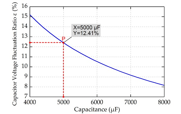
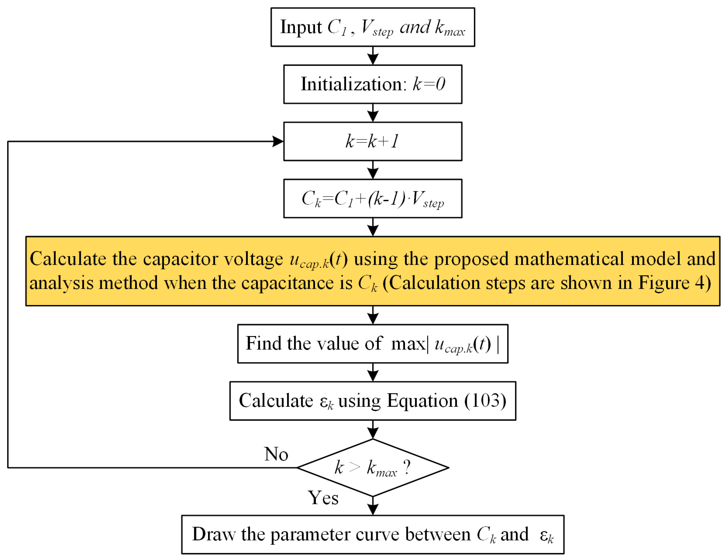
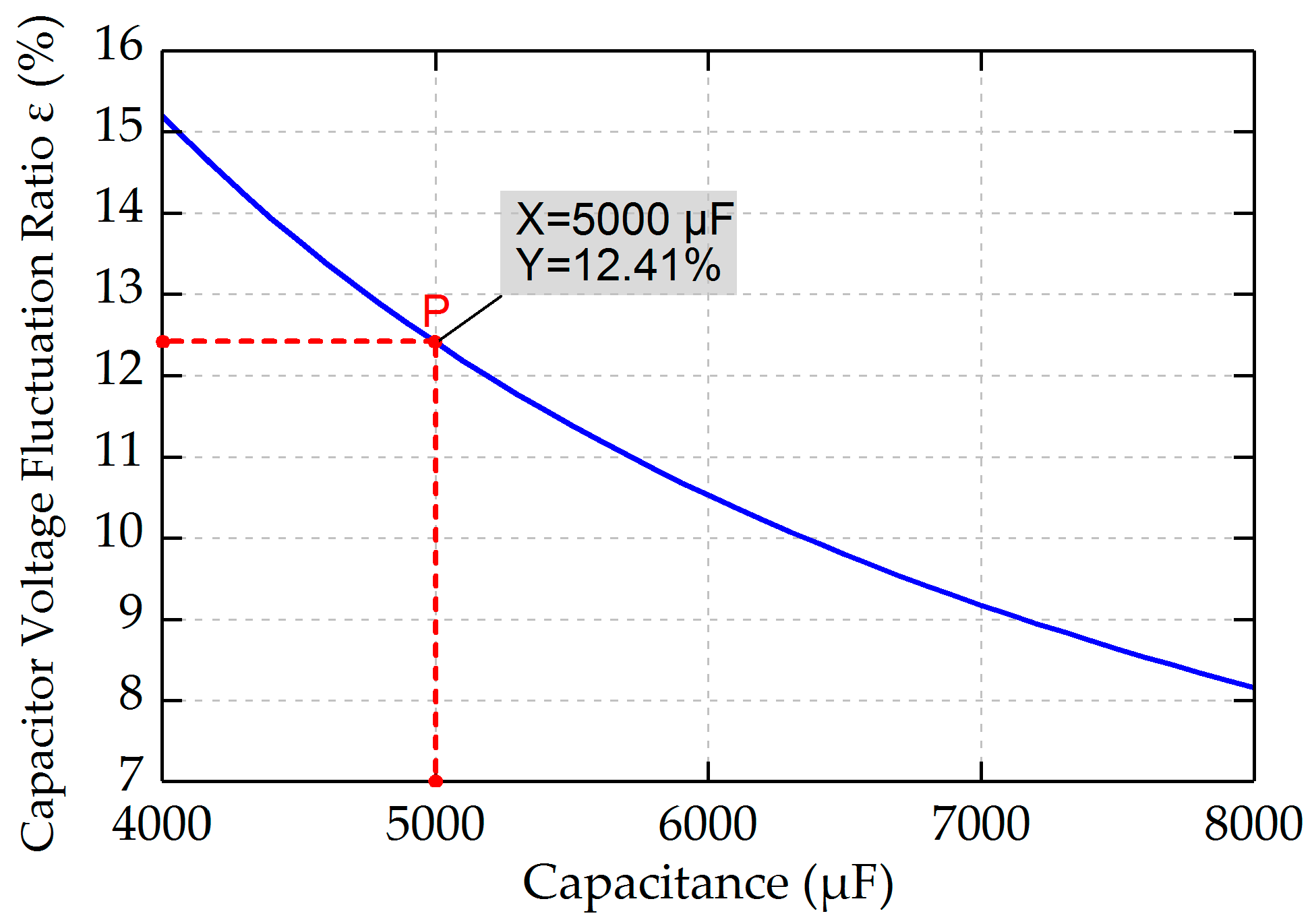
5.2. Capacitor Sizing For the MMC Connected to PMSG

The capacitors occupy approximately half the volume of MMC, and are the key components determining the performance of MMC.

The capacitor sizing mainly depends on the capacitor voltage ripples [28]. The capacitance should be large enough to limit the maximal voltage of capacitor below a given value; otherwise it may lead to IGBT breakdown and reduce the system reliability. However, choosing large capacitance will lead to high project cost and occupy a large area. Usually the appropriate capacitance should limit the capacitor voltage fluctuation ratio below 10%–15% [29]. Therefore, the calculation of the capacitor voltage is vital in the capacitor sizing.

According to Equations (54) and (55), the analytical expression of capacitor voltage can be expressed as:

$$u_{cap}(t)=u_{cap.dc}+\Delta u_{cap}(t)$$

(102)

where, $u_{cap.dc}$ is the DC component and $\Delta u_{cap}(t)$ is the fluctuation component.

Then, the capacitor voltage fluctuation ratio ε can be defined as follows [29]:

$$\epsilon =\frac{\max \left|\Delta u_{cap}(t)\right|}{u_{cap.dc}}\times 100\%=\frac{\max \left|u_{cap}(t)\right|-u_{cap.dc}}{u_{cap.dc}}\times 100\%$$

(103)

In the previous papers, the capacitor sizing method can be divided into two categories. One kind of the methods derives the capacitance requirement through the energy variation in the converter arms [30]. This kind of methods avoids deducing the equation of capacitor voltage ripple. Another kind of the methods sizes the capacitor by directly analyzing the capacitor voltage [29]. Since the mathematical expression of $u_{cap}(t)$ is complicated, the capacitor voltage fluctuation ratio ε is usually calculated by a lot of simplifications, which results in choosing an inappropriate value of capacitance. In addition, the previous capacitor sizing methods are proposed for the MMC used in HVDC transmission. The MMC connected to PMSG has different characteristics.

Since the proposed method can accurately calculate the capacitor voltages, it can be used for capacitor sizing. The paper focuses on the commonly used control strategy, in which the modulation controller uses the sinusoidal modulation method, and the 2nd harmonic circulating current is fully suppressed. There are optimization methods that can reduce the capacitance requirement. For example, in paper [31] an enhanced flat-topped modulation method is used to reduce the capacitance requirement. In paper [12] circulating current injection can also be used to suppress the capacitor voltage ripple. The influences of these optimization methods are out of the scope of this paper and will be studied in our future research.

From the analysis results in Section 5.1, for MMC connected to the PMSG-based WECS, the maximum fluctuation occurs when the wind speed reaches its rated value. Therefore, the capacitor should be sized under the rated wind speed.

The sizing procedure can be divided into two steps:

• Step 1: Draw the parameter curve based on the proposed mathematical model and analysis method shown in Section 4. The parameter curve describes the relationship between the capacitance and the capacitor voltage fluctuation ratio ε.
• Step 2: Select the appropriate value of capacitance according to the obtained parameter curve.

Figure 6 shows the flow chart of drawing the parameter curve, where k denotes the loop number. Firstly, the initial value of capacitance C₁, the step value of capacitance V_step and the max value of loop number k_max are inputted. Secondly, the loop number k is initialized to be zero. Then, k increases by 1. After that, the k-th value of the capacitance C_k is calculated. Next, the capacitor voltage $u_{cap.k}(t)$, when the capacitance is C_k, is calculated by using the proposed mathematical model and analysis method; the calculation step is shown in Figure 4. Then, the max value of $u_{cap.k}(t)$ can be obtained, and therefore the capacitor voltage fluctuation ratio ε_k can be easily calculated by Equation (103). Finally, after executing the loop k times, the parameter curve between C_k and ε_k can be dawn.

While drawing the parameter curve, the following three points should be noted:

(a)

The parameter curve is drawn by using the software, such as MATLAB.

(b)

The calculation of the capacitor voltage $u_{cap.k}(t)$ is the key step, the calculation steps are elaborated in Section 4.

(c)

To find the value of $\max \left|u_{cap.k}(t)\right|$, “max” function can be used in the program in MATLAB.

Figure 7 shows the parameter curve for the parameters shown in Table 1 and Table 2 (except the capacitance). It can be seen in the figure that the voltage fluctuation decreases with the increasing of capacitance. Therefore, for the parameters shown in the Table 1 and Table 2, if the voltage fluctuations are expected between 10–15%, the capacitance should be 4000–6000 μF; and if the voltage fluctuations are expected less than 10%, the capacitance should be greater than 6000 μF.

In this paper, the capacitance is chosen to be 5000 μF, and hence the capacitor voltage fluctuation will be lower than 12.41%.

6. Simulation Results

6.1. Simulation Model

In this section, simulations are carried out in MATLAB/Simulink (8.5.0.197613, MathWorks, Natick, MA, USA) in order to verify the accuracy of the proposed method and the correctness of the analysis. Figure 8 is the overall diagram of the simulation system. The simulation system is composed of three parts, which are the PSMG part, the MMC connected to PSMG part, and the AC grid part.

(a)

In the PMSG part, the wind turbine model is built based on the wind power formula. The mechanical shaft model uses a two-mass rotor model, with separate masses for the turbine and generator. The PSMG model is the typical model provided by MATLAB/Simulink. More details of this part can be referred to the paper [32].

(b)

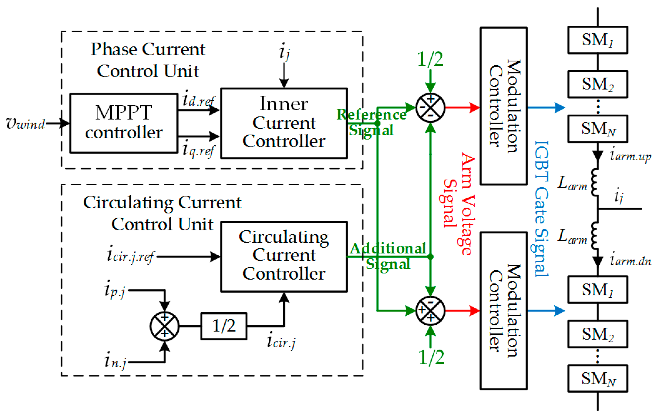
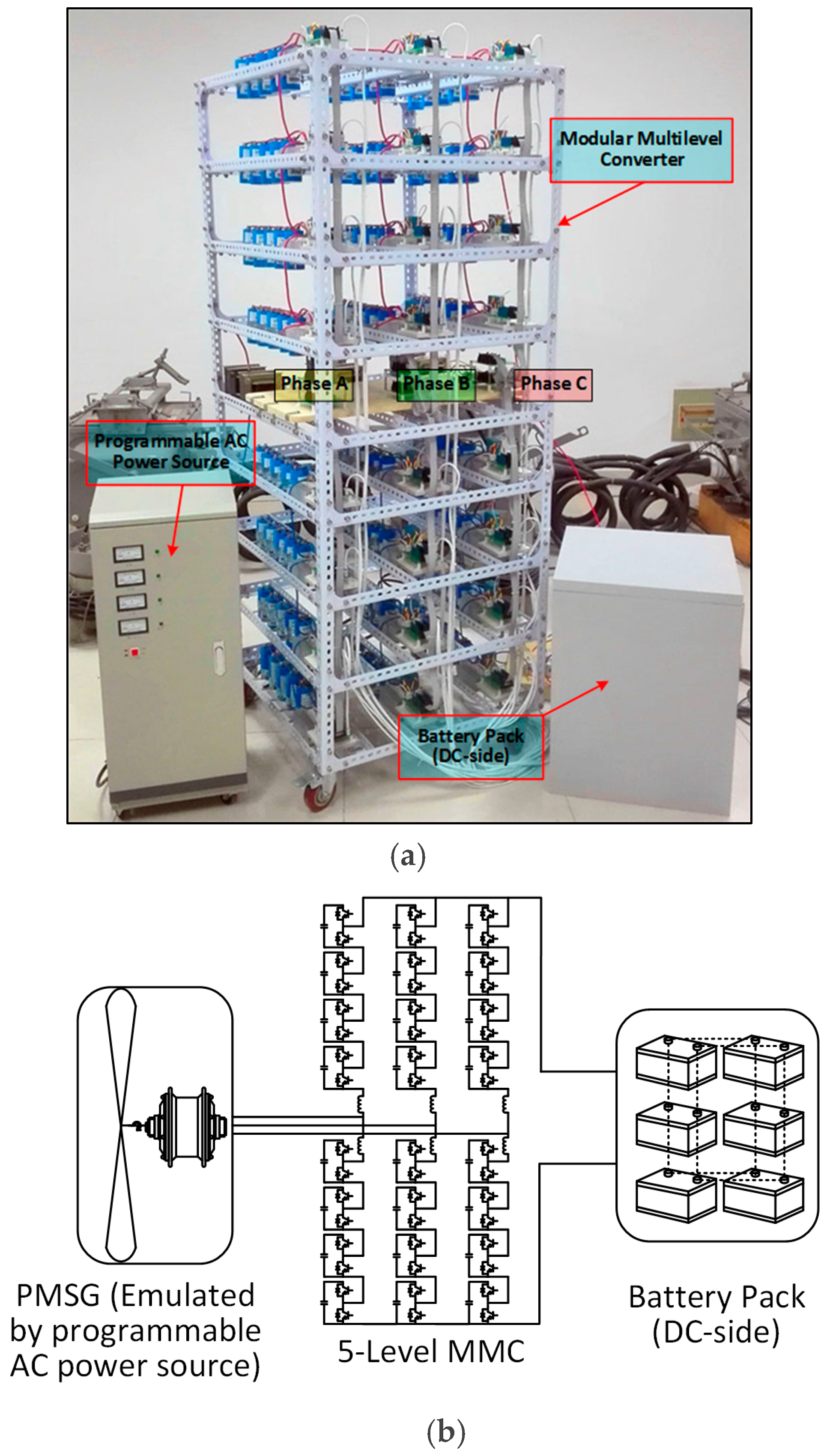
In the MMC connected to PSMG part, a five level MMC is built. As is shown in Figure 7, the sub-modules use half-bridge topology. MPPT controller is used to make the PMSG obtain the highest possible power from wind. PI controllers are used to track the reference values in the inner current controller and the circulating current controller. The IGBT gate signals (the switching function in the mathematic model) are obtained by comparing the arm voltage signals with the carrier signals. Details of this part can be referred to the paper [12].

(c)

In the AC grid part, the DC/AC converter is the traditional modular multilevel converter used in HVDC [17]. The AC grid is substituted with a three-phase AC source, in which the frequency is 50 Hz.

The simulation parameters of MMC and PMSG are listed in Table 1 and Table 2.

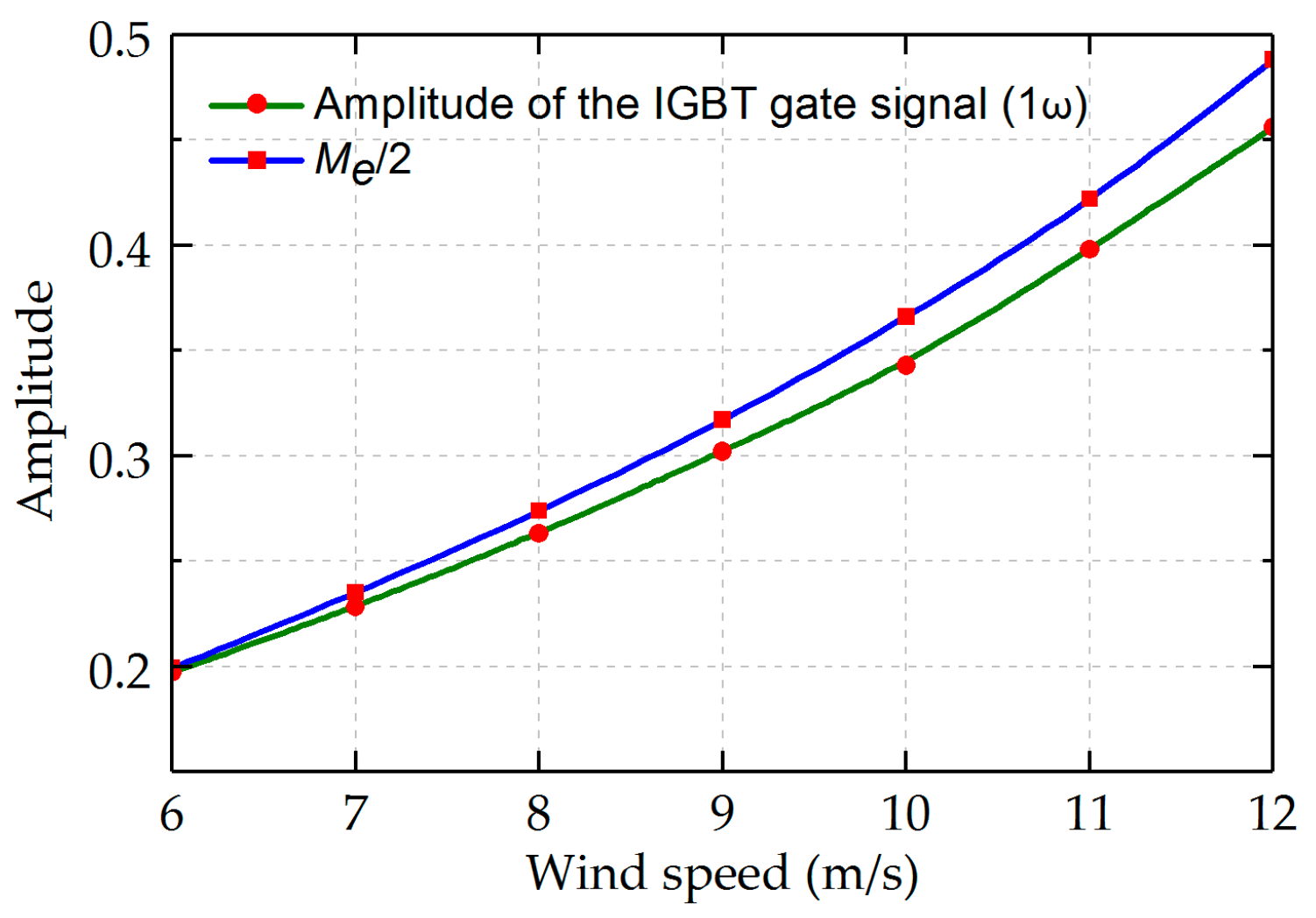
6.2. The Proposed Method to Calculate the Average Switching Functions

As mentioned above, conventionally, the half of the modulation ratio and the phase angle of EMF are taken as the amplitude and phase angle of the fundamental component in the average switching functions. In this paper, a more accurate method is adopted to calculate the average switching functions, in which the “reference signal” (shown in Figure 3) are considered as their fundamental components.

The simulation results for cases with different wind speed are shown in

Table 3. Results comparison between the proposed and traditional method.

Wind Speed (m/s)	IGBT Gate Signal (1ω)		Proposed Method (1ω)		Traditional Method (1ω)
	Ampl.	Ang. (°)	Ampl.	Ang. (°)	Ampl.	Ang. (°)
6	0.197	−89.6	0.198	−90.1	0.199	−100.7
8	0.263	−98.2	0.263	−98.6	0.274	−108.6
10	0.343	−109.2	0.342	−109.4	0.366	−117.8
12	0.456	−121.4	0.457	−121.5	0.488	−127.1

. In the table, the values of the amplitude and phase angle are obtained by processing the simulation data with the Fast Fourier Transform (FFT). In the first column, the simulation results show the amplitude and phase angle of the fundamental component in the IGBT gate signal, which can be considered as the benchmark. In the second column, the simulation results of the reference signals are shown. In the third column, the simulation results are the half of the modulation ratio and the phase angle of EMF. It can be seen that compare with the results in the third column, the results in the second column are more close to the results in the first column. This means that compared with the traditional method, the reference signal is more close to the fundamental component in the IGBT gate signal. Moreover, when the wind speed approaches its rated value, the errors between the half of the modulation ratio and the amplitude of the IGBT gate signal become larger.

Figure 9 further shows the error between the half of the modulation ratio and the amplitude of the fundamental component in the IGBT gate signal for cases with different wind speed. It can be seen that the error becomes larger as the wind speed increases. However, according to

Table 4. Simulation and calculation results at the wind speed of 12 m/s.

Item		Simulation Results/Calculation Results/Errors
		Amplitude		Phase Angle (°)
$e_{MMC.a}$ (V)	1ω	3912.4/3884.2	0.72%	52.8/53.1	0.57%
$i_a$ (A)	1ω	1061.7/1061.1	0.06%	90/90	0%
$I_{dc}$ (A)	dc	−618.9/−617.8	0.18%	N/A	N/A
$i_{cap.up}$ (A)	1ω	200.24/199.87	0.18%	−72.2/−71.7	0.69%
	2ω	124.74/124.65	0.07%	142.9/143.3	0.28%
	3ω	13.15/13.37	1.67%	161.1/157.8	2.05%
${\tilde{u}}_{cap.up}$ (V)	ω	253.85/254.32	0.19%	−162.2/−161.6	0.37%
	2ω	77.83/79.31	1.90%	54.1/53.4	1.29%
	3ω	5.78/5.69	1.90%	72.8/71.5	1.79%
$i_{arm.up}$ (A)	dc	−206.21/−205.93	0.14%	N/A	N/A
	ω	530.84/530.5	0.06%	−90/−90	0%
$S_{ref}$	ω	0.457/0.461	0.88%	58.5/58.0	0.85%
$S_{add}$	2ω	0.049/0.050	2.04%	68.2/67.7	0.73%

, the errors of the reference signals are small enough to be ignored under all the wind speeds operating conditions.

Figure 10 presents the comparisons between the simulation and calculation results. The red solid lines are obtained by simulation at the rated wind speed (12 m/s), and the blue dashed lines are obtained by the numerical calculation. The calculation results use the proposed analysis method, but the switching functions, in the analysis procedure, is calculated by traditional method. It can be seen that the simulation and calculation results have similar amplitudes and phase angles, but there still exist small errors. Therefore, more accurate method to calculate the average switching functions can be used to improve the accuracy of steady-state analysis. The calculation results using both of the proposed analysis method and the new method of calculating the average switching functions are shown in Figure 11 and Figure 12 in the next part.

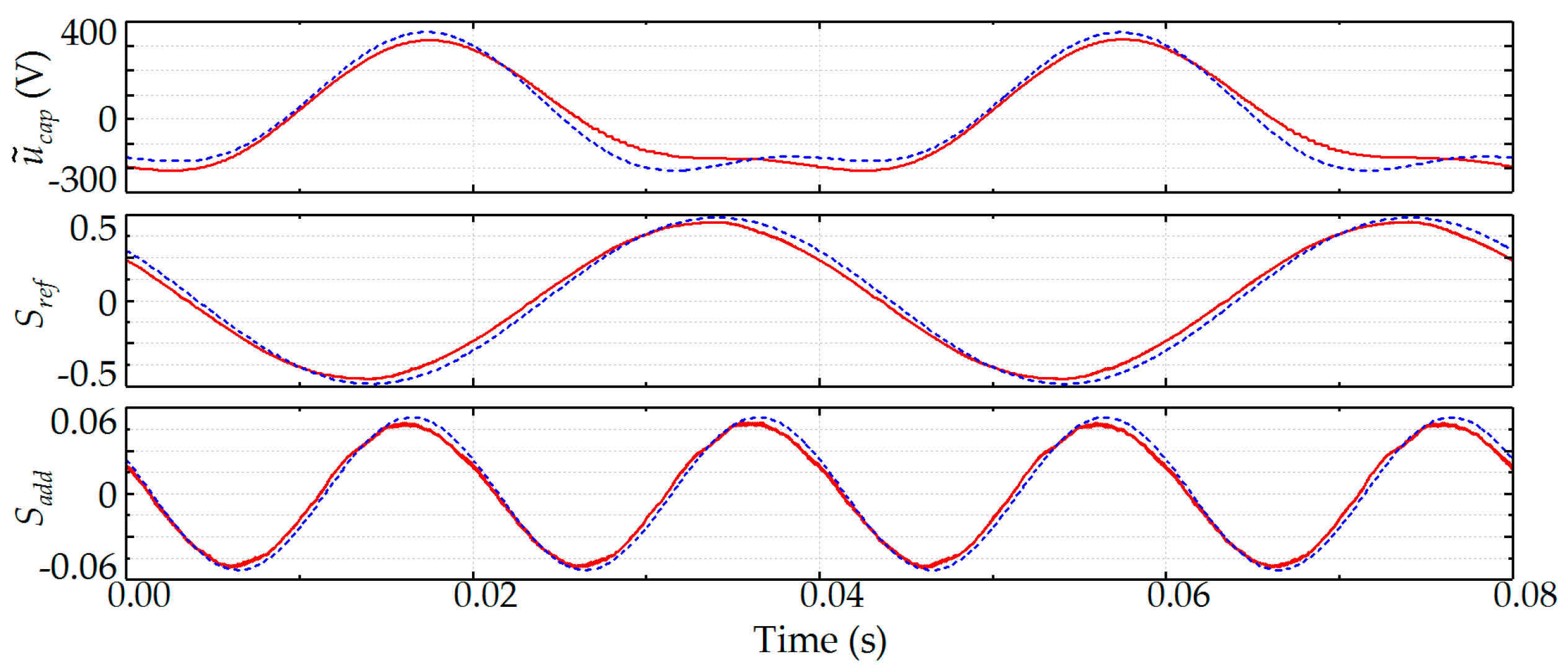
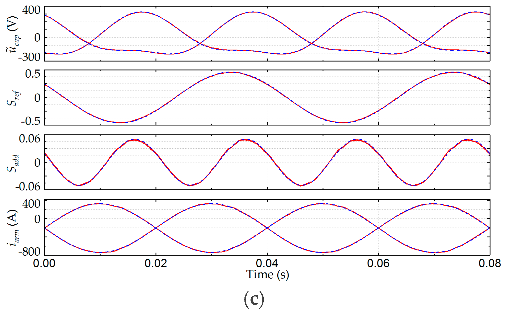
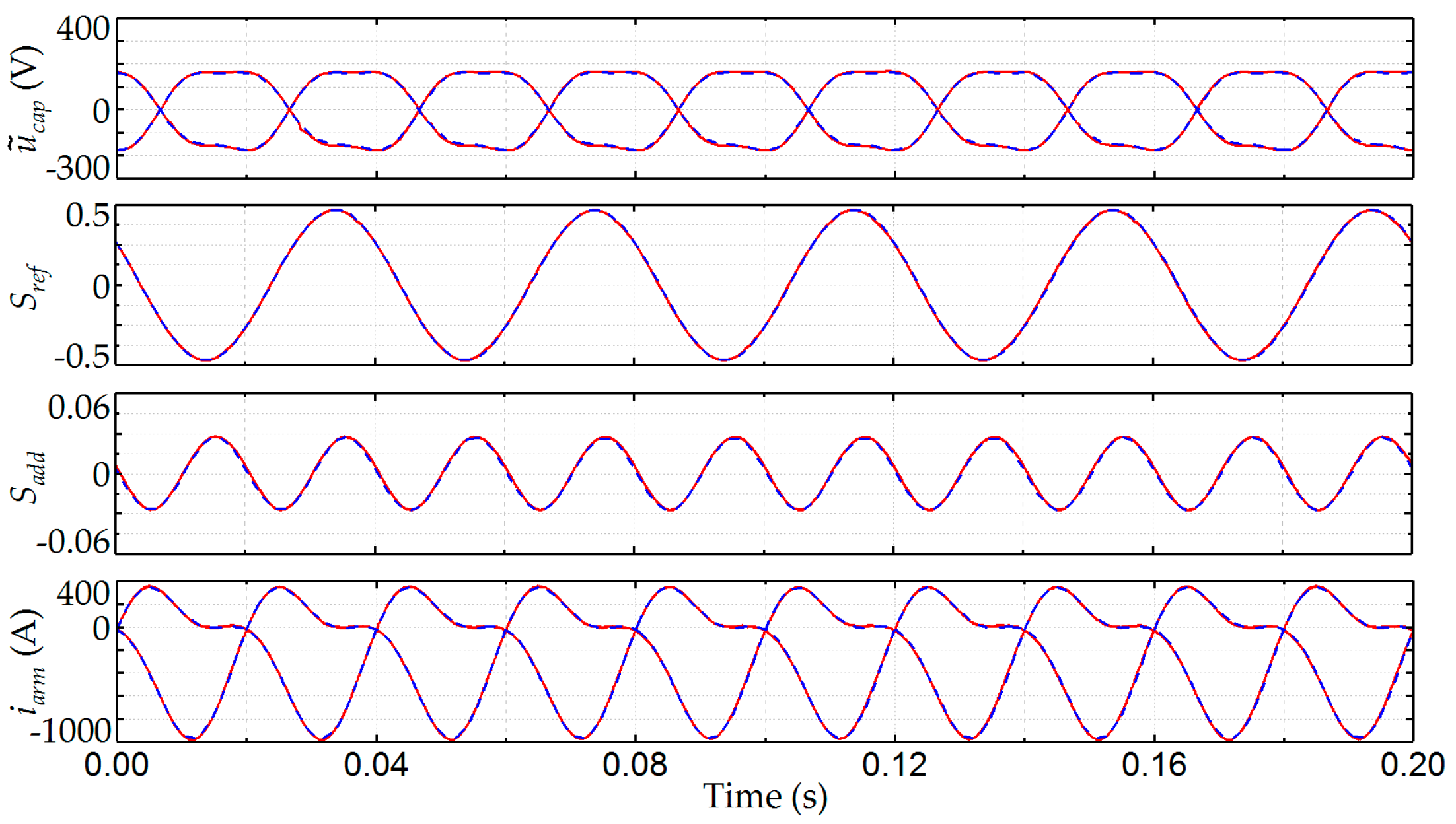
6.3. Simulation and Calculation Results for the Proposed Analysis Method

To verify the accuracy of the proposed steady-state analysis method, the simulation and calculation results for the cases with different wind speed are shown in Figure 11. In the subfigures, the red solid lines are the simulation results and the blue dashed lines are the calculation results. The circulating currents are suppressed to be zero. In each figure, from top to down, it presents the comparisons of the capacitor voltage ripples, the reference signals, the additional signals and the arm currents.

It can be seen that all the calculation results in Figure 11 fit well with the simulation results. Moreover, the simulation results in Figure 11c and Figure 10 are all carried out at the wind speed of 12 m/s. However, the calculation results in them, shown by the blue dashed lines, are obtained by using and without using the proposed method to calculate the average switching functions respectively. It can be seen that the calculation results obtained by using the proposed method, in Figure 11c, significantly have smaller errors. This means that by using more accurate way to calculate the average switching functions, the accuracy of the analysis method can be effectively improved.

To further verify the accuracy of the proposed steady-state analysis, the calculation results and their errors of more electrical quantities are shown in Table 4. The simulation and calculation are carried out at the rated wind speed.

It can be seen from Table 4 that the errors in the calculation results of both amplitudes and phase angles are small, and most of the errors, especially for the fundamental components, are less than 1%. This further proves that the proposed method has high accuracy.

In addition, in some papers such as [12], the circulating current is controlled to be a certain value (not zero) to suppress the capacitor voltage ripple. In order to prove that the proposed method also has high accuracy under this condition, Figure 12 presents the simulation and calculation results at the rated wind speed when $I_{cir}$ = 246.87 A and ${\theta }_{cir}$ = 5.5292 rad [12].

In Figure 12, since the circulating current is not zero, the arm current is not sinusoidal. It can be seen that the calculation results still fit well with the simulation results. This is because that the influence of circulating currents to other electrical quantities are considered in the stead-state analysis, and the additional signals, albeit small, are not ignored in the derivation procedure.

Moreover, the comparisons of calculation time between using the traditional method and using the proposed method to calculate the average switching function are shown in

Table 5. Comparison of calculation time.

Item	Calculation Time (s)
	100 Times	1000 Times	5000 Times	10000 Times
Traditional	0.3071	2.953	14.821	28.633
Accurate	0.3532	3.264	15.906	31.058

. The calculations are carried out in MATLAB software. The comparison results show that the calculation speed based on the proposed method is also very fast. This mainly benefits from that the unknown quantities in the average switch functions are obtainable at one stroke and no iteration is needed.

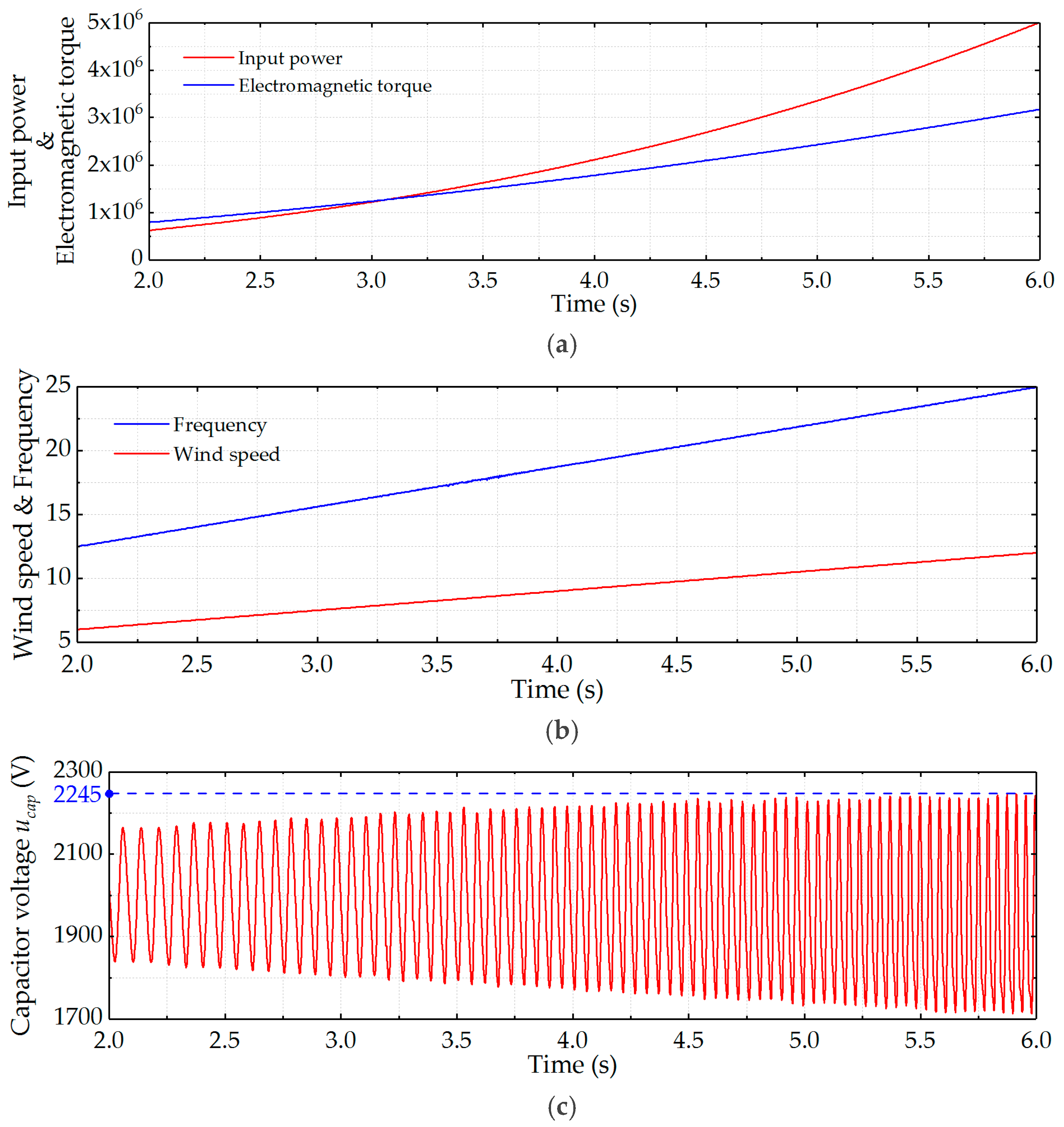
6.4. Simulation Results of the Capacitor Voltage Ripple

In Section 5, the characteristics of capacitor voltage ripple in the MMC connected to PMSG is analyzed. Different from the MMC applied in motor drives, for the MMC connected to PMSG, there is a positive correlation between the capacitor voltage ripple and the system frequency. In Figure 13, waveforms are shown when the wind speed increases from 6 m/s at 2 s to12 m/s at 6 s.

Figure 13a,b present the waveforms of the input power, electromagnetic torque, wind speed and system frequency. In Figure 13c, the circulating current is fully suppressed. The capacitor voltage ripple becomes larger as the wind speed increases, and the maximum fluctuation occurs when the wind speed reaches its rated value at 6 s. The simulation results coincide with the analysis in Section 5, which verifies the correctness of the analysis to capacitor voltage ripples. Moreover, the simulation proves that, for MMC connected to the PMSG-based WECS, capacitor voltage ripple suppression is not needed under low-frequency operation.

6.5. Simulation Results of the Capacitor Voltage Ripple under Different Capacitance Conditions

In order to verify the correctness of the proposed capacitor sizing method. Comparisons between the simulation and calculation results of the capacitor voltage ripple under the different capacitance are carried out in this section. Figure 14 shows the waveforms of capacitor voltages. The parameters are shown in Table 1 and Table 2 except that the capacitances from Figure 14a–d, are 4000 μF, 5000 μF, 6000 μF and 7000 μF respectively. Since the maximum fluctuation of the capacitor voltage occurs at the rated wind speed, all the simulations in Figure 14 are carried out at the rated wind speed.

Table 6. Comparison of the voltage fluctuation value ε.

Item	Voltage Fluctuation Value ε
	4000 μF	5000 μF	6000 μF	7000 μF
Simulation	15.25%	12.25%	10.45%	9.10%
Calculation	15.21%	12.41%	10.53%	9.21%

presents the comparisons. The voltage fluctuation value ε is obtained by using Equation (103), and the calculation results are obtained by parameter curve shown in Figure 9.

It can be seen from Table 6 that the calculation results meet well with the simulation results, which prove the accuracy of the proposed method. Therefore, for the parameters shown in Table 1 and Table 2, if the voltage fluctuations are expected between 10–15%, the capacitance should be 4000–6000 μF; and if the voltage fluctuations are expected less than 10%, the capacitance should be greater than 6000 μF.

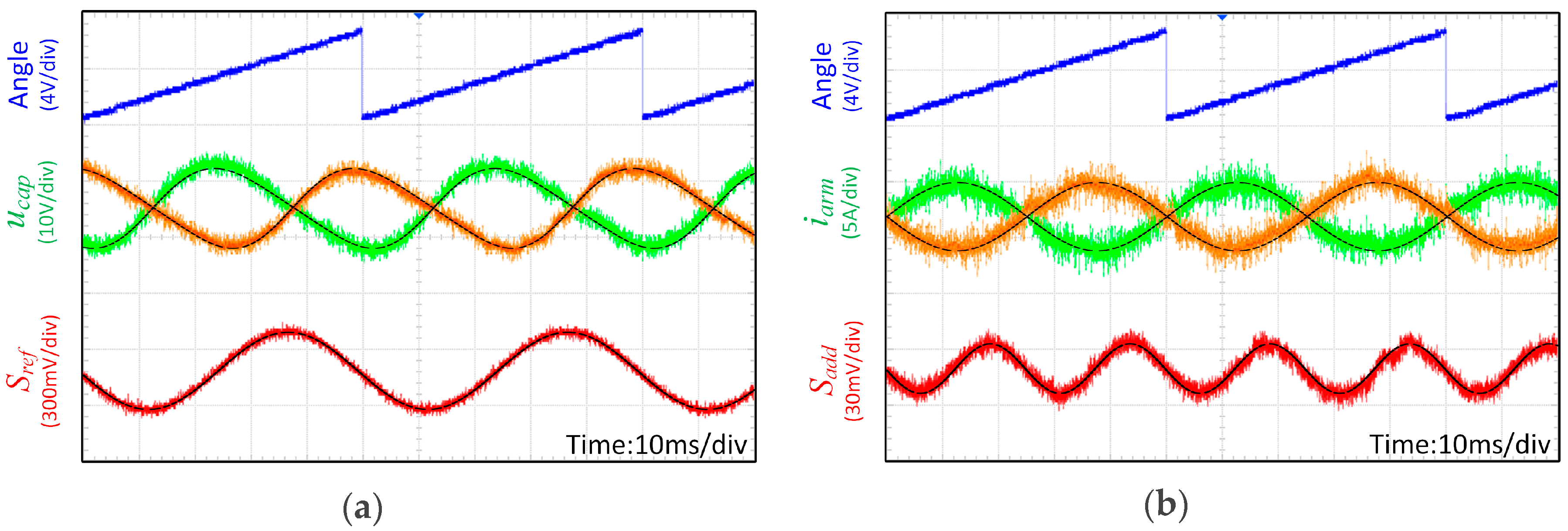
7. Experiment Validation

In order to further prove that the proposed method has high accuracy, a down-scaled prototype is implemented. The photograph of the prototype is presented in Figure 15a, and its diagram is shown in Figure 15b.

The experiment part intends to verify that the calculation results in the MMC are accurate, and only focuses on the steady state. Since the composition of torque in PMSG is zero in the steady state, the PMSG can be taken as a voltage source for the MMC. Therefore, the PMSG part is emulated by the programmable power source, in which the wind turbine characteristics are programmed to emulate a generator operating at variable speed and variable voltage [33]. The experiment parameters of the emulated PMSG is shown in Table 2. In the MMC part, each arm contains four sub-modules. The control scheme of MMC is the same as it in the simulation part, which can be referred in paper [12]. For the hardware realization of the control scheme, the modulation parts are realized in Field Programmable Gate Array (FPGA) chip, called EP4CE30F23 (Altera Corporation, San Jose, CA, USA); the inner-current controller and circulating current controller are realized by Digital Signal Processor (DSP) chip, called TMS320f28335 (Texas Instruments, Dallas, TX, USA). The experiment parameters of MMC are shown in Table 1.

In Figure 16, Figure 17 and Figure 18, the comparisons between the experiment waveforms and the calculation results are shown. The blue lines are the waveforms of benchmark angles, used to observe the phase angle of acquired signals. The red lines are the waveforms of reference and additional signals. The benchmark angles, reference signals and additional signals are first acquired by FPGA, and then they are outputted to oscilloscope via digital-analogue (D/A) converter. The orange and green lines are the waveforms of capacitor voltages and arm currents. The black dashed lines are the calculation results obtained by using the proposed method.

Figure 16 shows the comparisons when the prototype works under the rated wind speed. The system frequency is 40 Hz. In Figure 17 and Figure 18, the prototype works at the wind speeds of 9 m/s and 6m/s respectively, in which the system frequencies are 30 Hz and 20 Hz respectively. From Figure 16, Figure 17 and Figure 18, it can be seen that the calculation results fit well with the experiment waveforms, which further validate the accuracy of the proposed analysis method.

8. Conclusions

This paper proposes a steady-state analysis method for MMC connected to the PMSG-based WECS. All the electrical quantities in MMC, including the amplitudes, phase angles and their harmonics, can be easily obtained according to the proposed method step by step. The proposed method can help design the parameters and optimize the operation of MMC used in the PMSG-based WECS.

The analysis method is based on the proposed d-q frame mathematical model of the MMC connected to PMSG. By using the d-q frame, the time-varying quantities are transformed into constant quantities, which simplifies the derivation. Due to this, the equivalent resistances in the MMC arms can be considered, and the algebraic solution of non-linear equations can be obtained to calculate the unknowns in the average switching functions.

A more accurate method to calculate the average switching functions are used in this paper. The comparisons between the simulation and calculation results show that the accuracy of analysis can be effectively improved by using the proposed method.

The analysis to capacitor voltage ripple concludes that there is a positive correlation between the capacitor voltage ripple and the system frequency for MMC connected to the PMSG-based WECS. Therefore, the capacitor voltage ripple suppression is not needed under low-frequency operation, which is different from the MMC applied in motor drives. In addition, a capacitor sizing method is also proposed in this paper, and is verified by the simulation results.

Comparisons between the simulation and calculation results have shown that the proposed steady-state analysis method has high accuracy, and most of the calculation errors, especially for the fundamental components, are less than 1%. Experiments carried out by a down-scaled prototype further prove that the proposed method has high accuracy under different operating condition.

References

1. Chavira, F.; Ortega-Cisneros, S.; Rivera, J. A Novel Sliding Mode Control Scheme for a PMSG-Based Variable Speed Wind Energy Conversion System. Energies 2017, 10, 1476. [Google Scholar] [CrossRef]
2. Yaramasu, V.; Wu, B.; Sen, P.C.; Kouro, S.; Narimani, M. High-power Wind Energy Conversion Systems: State-of-the-art and Emerging Technologies. Proc. IEEE 2015, 103, 740–788. [Google Scholar] [CrossRef]
3. Zhao, L.; Adamiak, K. Numerical Simulation of the Effect of EHD Flow on Corona Discharge in Compressed Air. IEEE Trans. Ind. Appl. 2013, 49, 298–304. [Google Scholar] [CrossRef]
4. Cheng, X.; Lee, W.J.; Sahni, M.; Cheng, Y.; Lee, L.K. Dynamic Equivalent Model Development to Improve the Operation Efficiency of Wind Farm. IEEE Trans. Ind. Appl. 2016, 52, 2759–2767. [Google Scholar] [CrossRef]
5. Yaramasu, V.; Dekka, A.; Durán, M.J.; Kouro, S.; Wu, B. PMSG-based wind energy conversion systems: Survey on power converters and controls. IET Electr. Power Appl. 2017, 11, 956–968. [Google Scholar] [CrossRef]
6. Yuan, X. A Set of Multilevel Modular Medium-Voltage High Power Converters for 10-MW Wind Turbines. IEEE Trans. Sustain. Energy 2014, 5, 524–534. [Google Scholar] [CrossRef]
7. Abu-Rub, H.; Holtz, J.; Rodriguez, J.; Ge, B. Medium-Voltage Multilevel Converters-State of the Art, Challenges, and Requirements in Industrial Applications. IEEE Trans. Ind. Electron. 2010, 57, 2581–2596. [Google Scholar] [CrossRef]
8. Hagiwara, M.; Nishimura, K.; Akagi, H. A Medium-Voltage Motor Drive with a Modular Multilevel PWM Inverter. IEEE Trans. Power Electron. 2010, 25, 1786–1799. [Google Scholar] [CrossRef]
9. Antonopoulos, A.; Angquist, L.; Norrga, S.; Ilves, K.; Harnefors, L.; Nee, H.P. Modular Multilevel Converter AC Motor Drives with Constant Torque from Zero to Nominal Speed. IEEE Trans. Ind. Appl. 2014, 50, 1982–1993. [Google Scholar] [CrossRef]
10. Iversen, T.M.; Gjerde, S.S.; Undeland, T. Multilevel converters for a 10 MW, 100 kV transformer-less offshore wind generator system. In Proceedings of the 15th European Conference on Power Electronics and Applications (EPE), Lille, France, 2–6 September 2013. [Google Scholar]
11. Liu, H.; Ma, K.; Loh, P.C.; Blaabjerg, F. Online Fault Identification Based on an Adaptive Observer for Modular Multilevel Converters Applied to Wind Power Generation Systems. Energies 2015, 8, 7140–7160. [Google Scholar] [CrossRef]
12. Wang, M.; Hu, Y.; Zhao, W.; Wang, Y; Chen, G. Application of modular multilevel converter in medium voltage high power permanent magnet synchronous generator wind energy conversion systems. IET Renew. Power Gener. 2016, 10, 824–833. [Google Scholar] [CrossRef]
13. Holtsmark, N.; Bahirat, H.J.; Molinas, M.; Mork, B.A.; Hoidalen, H.K. An All-DC Offshore Wind Farm with Series-Connected Turbines: An Alternative to the Classical Parallel AC Model? IEEE Trans. Ind. Electron. 2013, 60, 2420–2428. [Google Scholar] [CrossRef]
14. Parastar, A.; Kang, Y.C.; Seok, J.K. Multilevel Modular DC/DC Power Converter for High-Voltage DC-Connected Offshore Wind Energy Applications. IEEE Trans. Ind. Electron. 2015, 62, 2879–2890. [Google Scholar] [CrossRef]
15. Liu, H.; Guo, H.; Liang, J.; Qi, L. Impedance-Based Stability Analysis of MVDC Systems Using Generator-Thyristor Units and DTC Motor Drives. IEEE J. Emerg. Sel. Top. Power Electron. 2017, 5, 5–13. [Google Scholar] [CrossRef]
16. Ilves, K.; Antonopoulos, A.; Norrga, S.; Nee, H.P. Steady-State Analysis of Interaction between Harmonic Components of Arm and Line Quantities of Modular Multilevel Converters. IEEE Trans. Power Electron. 2012, 27, 57–68. [Google Scholar] [CrossRef]
17. Song, Q.; Liu, W.; Li, X.; Rao, H.; Xu, S.; Li, L. A Steady-State Analysis Method for a Modular Multilevel Converter. IEEE Trans. Power Electron. 2013, 28, 3702–3713. [Google Scholar] [CrossRef]
18. Vasiladiotis, M.; Cherix, N.; Rufer, A. Accurate Capacitor Voltage Ripple Estimation and Current Control Considerations for Grid-Connected Modular Multilevel Converters. IEEE Trans. Power Electron. 2014, 29, 4568–4579. [Google Scholar] [CrossRef]
19. Wang, J.; Liang, J.; Gao, F.; Dong, X.; Wang, C.; Zhao, B. A Closed-Loop Time-Domain Analysis Method for Modular Multilevel Converter. IEEE Trans. Power Electron. 2017, 32, 7494–7508. [Google Scholar] [CrossRef]
20. Ilves, K.; Antonopoulos, A.; Harnefors, L.; Norrga, S.; Angquist, L.; Nee, H.P. Capacitor Voltage Ripple Shaping in Modular Multilevel Converters Allowing for Operating Region Extension. In Proceedings of the IECON 2011—37th Annual Conference on IEEE Industrial Electronics Society, Melbourne, Australia, 7–10 November 2011. [Google Scholar]
21. Ma, C.; Qu, L. Multiobjective Optimization of Switched Reluctance Motors Based on Design of Experiments and Particle Swarm Optimization. IEEE Trans. Energy Convers. 2015, 30, 1144–1153. [Google Scholar] [CrossRef]
22. Kunjumuhammed, L.P.; Pal, B.C.; Gupta, R.; Dyke, K.J. Stability Analysis of a PMSG-Based Large Offshore Wind Farm Connected to a VSC-HVDC. IEEE Trans. Energy Convers. 2017, 32, 1166–1176. [Google Scholar] [CrossRef]
23. Yazdani, A.; Iravani, R. A Neutral-Point Clamped Converter System for Direct-Drive Variable-Speed Wind Power Unit. IEEE Trans. Energy Convers. 2006, 21, 596–607. [Google Scholar] [CrossRef]
24. Debnath, S.; Saeedifard, M. A New Hybrid Modular Multilevel Converter for Grid Connection of Large Wind Turbines. IEEE Trans. Sustain. Energy 2013, 4, 1051–1064. [Google Scholar] [CrossRef]
25. Jung, J.J.; Lee, H.J.; Sul, S.K. Control Strategy for Improved Dynamic Performance of Variable-Speed Drives with Modular Multilevel Converter. IEEE J. Emerg. Sel. Top. Power Electron. 2015, 3, 371–380. [Google Scholar] [CrossRef]
26. Yu, L.; Li, R.; Xu, L. Distributed PLL-based Control of Offshore Wind Turbine Connected with Diode-Rectifier based HVDC Systems. IEEE Trans. Power Deliv. 2017. [Google Scholar] [CrossRef]
27. He, L.; Zhang, K.; Xiong, J.; Fan, S.; Xue, Y. Low-Frequency Ripple Suppression for Medium-Voltage Drives Using Modular Multilevel Converter with Full-Bridge Submodules. IEEE J. Emerg. Sel. Top. Power Electron. 2016, 4, 657–667. [Google Scholar] [CrossRef]
28. Merlin, M.M.; Green, T.C. Cell Capacitor Sizing in Multilevel Converters: Cases of the Modular Multilevel Converter and Alternate Arm Converter. IET Power Electron. 2015, 8, 350–360. [Google Scholar] [CrossRef]
29. Xu, Z.; Xiao, H.; Zhang, Z. Selection Methods of Main Circuit Parameters for Modular Multilevel Converters. IET Renew. Power Gener. 2016, 10, 788–797. [Google Scholar] [CrossRef]
30. Li, R.; Fletcher, J.E. A Hybrid Modular Multilevel Converter with Novel Three-Level Cells for DC Fault Blocking Capability. IEEE Trans. Power Deliv. 2015, 30, 2017–2026. [Google Scholar] [CrossRef]
31. Li, R.; Fletcher, J.E.; Xu, L.; Williams, B.W. Enhanced Flat-Topped Modulation for MMC Control in HVDC Transmission Systems. IEEE Trans. Power Deliv. 2017, 32, 152–161. [Google Scholar] [CrossRef] [Green Version]
32. Miller, N.W.; Sanchez-Gasca, J.J.; Price, W.W.; Delmerico, R.W. Dynamic modeling of GE 1.5 and 3.6 MW wind turbine-generators for stability simulations. In Proceedings of the 2003 IEEE Power Engineering Society General Meeting, Toronto, ON, Canada, 13–17 July 2003. [Google Scholar]
33. Diaz, M.; Cardenas, R.; Espinoza, M.; Rojas, F.; Mora, A.; Clare, J.C.; Wheeler, P. Control of Wind Energy Conversion Systems Based on the Modular Multilevel Matrix Converter. IEEE Trans. Ind. Electron. 2017, 64, 8799–8810. [Google Scholar] [CrossRef]
Figure 1. Diagram of MMC connected to the PMSG-based WECS.
Energies 11 00461 g001
Figure 2. D-q frame equivalent circuit of MMC connected to the PMSG-based WECS.
Energies 11 00461 g002
Figure 3. Control scheme of MMC connected to the PMSG-based WECS.
Energies 11 00461 g003
Figure 4. Flow chart of the proposed steady-state analysis method.
Energies 11 00461 g004
Figure 5. Steady-state analysis results of fluctuation magnitude at different frequencies.
Energies 11 00461 g005
Figure 6. Flow chart of drawing the parameter curve.
Energies 11 00461 g006
Figure 7. Parameter curve between the capacitance and the voltage fluctuation ratio.
Energies 11 00461 g007
Figure 8. Diagram of the simulation model.
Energies 11 00461 g008
Figure 9. Comparisons between modulation ratio and amplitude of IGBT gate signal.
Energies 11 00461 g009
Figure 10. Comparisons between the simulation and calculation results using the traditional method to calculate the average switching function.
Energies 11 00461 g010
Figure 11. Comparisons between the simulation results and calculation results. (a) The wind speed is 6 m/s; (b) the wind speed is 9 m/s; (c) the wind speed is 12 m/s (rated wind speed).
Energies 11 00461 g011aEnergies 11 00461 g011b
Figure 12. Comparisons between the simulation results and the calculation results.
Energies 11 00461 g012
Figure 13. Waveforms when wind speed increases from 6 m/s at 2 s to12 m/s at 6 s. (a) Input power and electromagnetic torque; (b) wind speed and system frequency; (c) capacitor voltage.
Energies 11 00461 g013
Figure 14. Waveforms of capacitor voltages under the different capacitance at the rated wind speed. (a) C = 4000 μF; (b) C = 5000 μF; (c) C = 6000 μF; (d) C = 7000 μF.
Energies 11 00461 g014
Figure 15. Down-scaled prototype for MMC connected to the PMSG-based WECS. (a) Photograph, (b) Diagram.
Energies 11 00461 g015
Figure 16. Comparisons between the experiment waveforms and calculation results when the wind speed is 12 m/s. (a) Capacitor voltage ripples and reference signal; (b) Arm currents and additional signal.
Energies 11 00461 g016
Figure 17. Comparisons between the experiment waveforms and calculation results when the wind speed is 9 m/s. (a) Capacitor voltage ripples and reference signal; (b) Arm currents and additional signal.
Energies 11 00461 g017
Figure 18. Comparisons between the experiment waveforms and calculation results when the wind speed is 6 m/s. (a) Capacitor voltage ripples and reference signal; (b) Arm currents and additional signal.
Energies 11 00461 g018