Modulation Strategy of a 3 × 5 Modular Multilevel Matrix Converter


School of Electrical Engineering, Northeast Electric Power University, Jilin 132012, China
*
Author to whom correspondence should be addressed.
Energies 2018, 11(2), 464; https://doi.org/10.3390/en11020464
Submission received: 2 January 2018
/
Revised: 8 February 2018
/
Accepted: 9 February 2018
/
Published: 23 February 2018
Abstract
:In this paper, a modulation strategy of a 3 × 5 modular multilevel matrix converter (M3C) is proposed. The circuit of 3 × 5 M3C is firstly introduced. Then, operation rules of 3 × 5 M3C are illustrated, and a connection pattern of branches is determined based on these rules. Different voltage states in the input and output side can be achieved by different connection patterns. These voltage states are represented in the form of vector. It is hard to synthesize five-phase output with the three-level synthesis method. Therefore, the five-level synthesis method is adopted in this paper; i.e., is the branch states have been increased. Ten effective vectors and a zero vector are selected based on the five-level synthesis method. With this modulation strategy, we achieve output line-to-line voltages that are in line with the trend of a sine wave. The segment division and duty cycle calculation are very simple, and the modulation strategy can be implemented easily. The simulation model of 3 × 5 M3C is constructed based on Matlab/Simulink, and the corresponding experimental platform is set up. The results of simulation and experiment show that the proposed method is reasonable and correct.
1. Introduction
In recent years, more and more attention has been paid to the research on a multiphase AC drive system. Compared with the three-phase motor, the multi-phase motor system has the advantages of small torque fluctuation, high power density, high efficiency, fault tolerant operation and low voltage high power, etc. It has developed rapidly in fields such as electric/hybrid electric vehicle drives, electric ship propulsion, aircraft drives, locomotive traction, offshore wind generation, aerospace drives and some high power industrial applications and other applications [1,2,3,4,5,6]. The advantages are obvious. The main reason for these advantages is that the power level of each phase in a multi-phase system was reduced, and the fault-tolerant performance was improved. Due to the development of multi-phase motors, new requirements for the development of multiphase matrix converter are also proposed.
Modular multilevel converter (MMC) and M3C all belong to multilevel converters. MMC is composed of cascaded half-bridge converters, and it mainly focuses on DC/AC conversion [7,8]. In order to achieve AC/AC conversion, two back-to-back MMCs as shown in [9] should be adopted. M3C is a new cascade H-bridge AC-AC converter [10]. Compared with MMC, it can realize AC/AC conversion with fewer branches, and no additional high frequency common mode voltage and current are needed in the aspect of low frequency control. M3C also has some other advantages such as full modularity, simple extension to high voltage levels, control flexibility, better harmonic quality and redundancy, and the fact that several failed modules do not necessarily cause system shutdown [11,12,13]. These unique advantages make it very suitable for high-power low-speed motor drives and high-power wind energy conversion systems [11,14,15].
3 × 5 M3C is developed by a 3 × 3 M3C. Due to the special structure of the 3 × 5 M3C, it not only takes into account traditional matrix converters and modular multi-level advantages, but also, each branch is relatively independent. Therefore, each branch can be seen as a single-phase cascade inverter, which makes its control strategy more flexible. 3 × 5 phase M3C is very suitable for the five-phase high-power low-speed drive systems and other five-phase AC/AC conversion applications. Because of the multi-phase motor’s safety, its reliability is higher than the three-phase motor. When subjected to more in-depth studies, 3 × 5 M3C will have very broad prospects.
At present, research on 3 × 3 M3C has achieved some progress, the authors of [11] discuss the application of M3C in wind energy conversion systems. Good steady state and dynamic performance are achieved, phase shifted PWM scheme is adopted to synthesize the voltage, and the modulation is simple to implement. However, the calculation of modulation wave for each H-bridge cell is complex. A general nonlinear multivariable optimization model is set up to optimize the branch current configuration after the branch loss described in [12]. A smaller system power capability loss after the branch fault is achievable; however, the internal circulating current component is not mentioned, and it is difficult to suppress by current feedback. An integrated current-energy model is formulated and the decoupled active and reactive power control is achieved in [10]. In [14], a control method based on capacitor voltage estimation is applied so that capacitor voltage measurement is not needed in the high-level control state-space model of the converter. In both papers, a control system is established. An integrated perturbation analysis and sequential quadratic programming solver is used to reduce the computational complexity in [13]. A cost function that considers error terms is provided and the dynamics response of capacitor voltage average value is improved in [15]. A prediction method is adopted in both papers.
However, a study of 3 × 5 M3C has not been carried out yet. 3 × 5 M3C can be seen as an expansion of 3 × 3 M3C in the topological structure, and therefore analysis of three-phase M3C can be a reference for five-phase M3C. However, the five-phase M3C is essentially different from the three-phase M3C. Input and outputs of three-phase M3C can be interchangeable. However, due to the five-phase M3C with the three-phase input and five-phase output, the input and output side cannot be directly interchangeable. The biggest difference between the three-phase and five-phase matrix converter is that all the possible bridge arm connections can be used to synthesize the required combinations of input/output vectors in three-phase M3C, while the five-phase matrix converter very strictly adheres to the bridge-arm connection structure. Not all bridge connections are compliance with the requirement of input/output vector combination, and the whole length of the vector cannot meet the requirement of synthesizing the output voltage. For the three-phase M3C, the conversion can be realized by only one H-bridge cell in the effective state in a working arm branch as in [16]. In this case, the output line voltage is three-level. Because, for five-phase M3C, the three-level synthesis method is no longer applicable, a five-level method is adopted in this paper. The number of effective H-bridge cells is no longer the same according to different combination of vectors. The selection of a basic vector is determined by the five-level synthesis method. Ten effective vectors and a zero vector are adopted in the output side. The segment division and duty cycle calculation of the proposed method are very simple, and the modulation strategy can be easily implemented. Finally, the feasibility of the proposed 3 × 5 M3C and its control strategy is verified by simulation and experiment.
2. Basic Operation Principles of 3 × 5 M3C
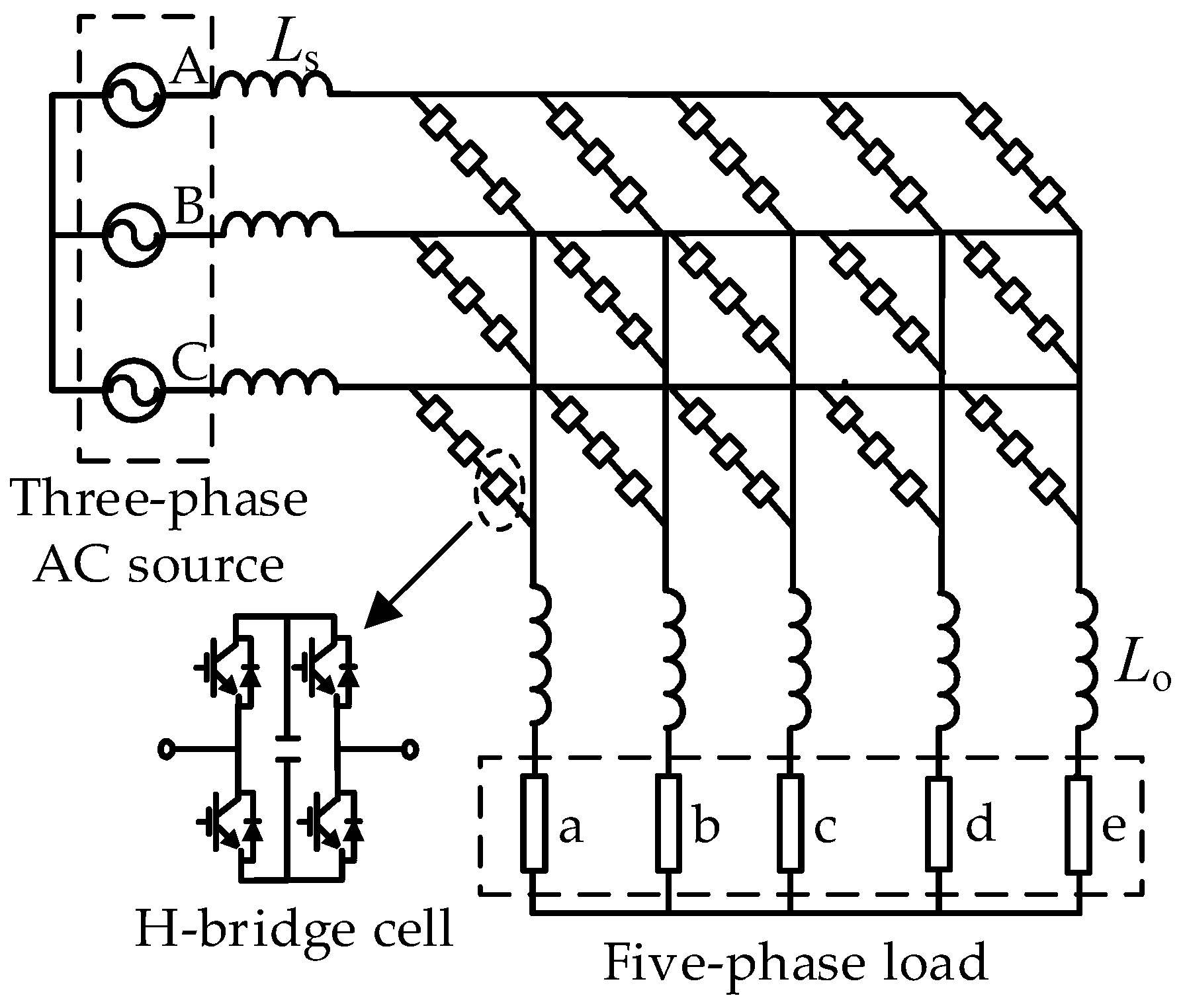
3 × 5 M3C is a 3 × 5 switch matrix consists of 15 cascaded H-bridge branches, and each branch is composed of several H-bridge cells. Its circuit topology is shown in Figure 1. In this paper, there are three H-bridge cells in each branch, the input three-phase are denoted as “A, B, C” and the output five-phase system are denoted as “a, b, c, d, e”, Ls and Lo are filter inductors of input and output side.
Similar to the constraint conditions of 3 × 3 M3C, 3 × 5 M3C branch connections need to fulfill the following conditions:
- Due to the existence of inductor on input and output side of 3 × 5 M3C, the continuity of current on both sides should be ensured so that the input/output phase should not open. Otherwise, the high voltage induced by the inductance current in the open circuit will damage the switch device;
- In order to effectively avoid the high voltage stress on the IGBT element, the total charge through the open switching unit should not exceed the capacitance voltage Ucap.
- All branches of M3C in the switch matrix should not be short-circuited, otherwise, short-circuit current will damage the converter.
Under the above constraints, the following basic principles should be followed when the space vector combination is selected:
- There is at most one branch connection between any input and output phase.
- If any of the inputs are only connected to one of the outputs, the remaining two-phase inputs must also be connected to this output phase.
- The adjacent two phases of outputs must be connected to the same input phase, otherwise the required output voltage cannot be synthesized.
Accordingly, the switch combination table can be obtained as follows.
As can be seen from Table 1, seven branch connections are required to synthesize the input/output side voltages. There are theoretically 573 feasible combinations; each switch has 3 valid states, namely, +1, −1, and 0. Only one H-bridge cell is selected for output in a branch. For example, there are 37 = 2187 possible combinations of connections for the 7 branches, and the total number of switch combinations is 573 × 2187 = 1,253,151.
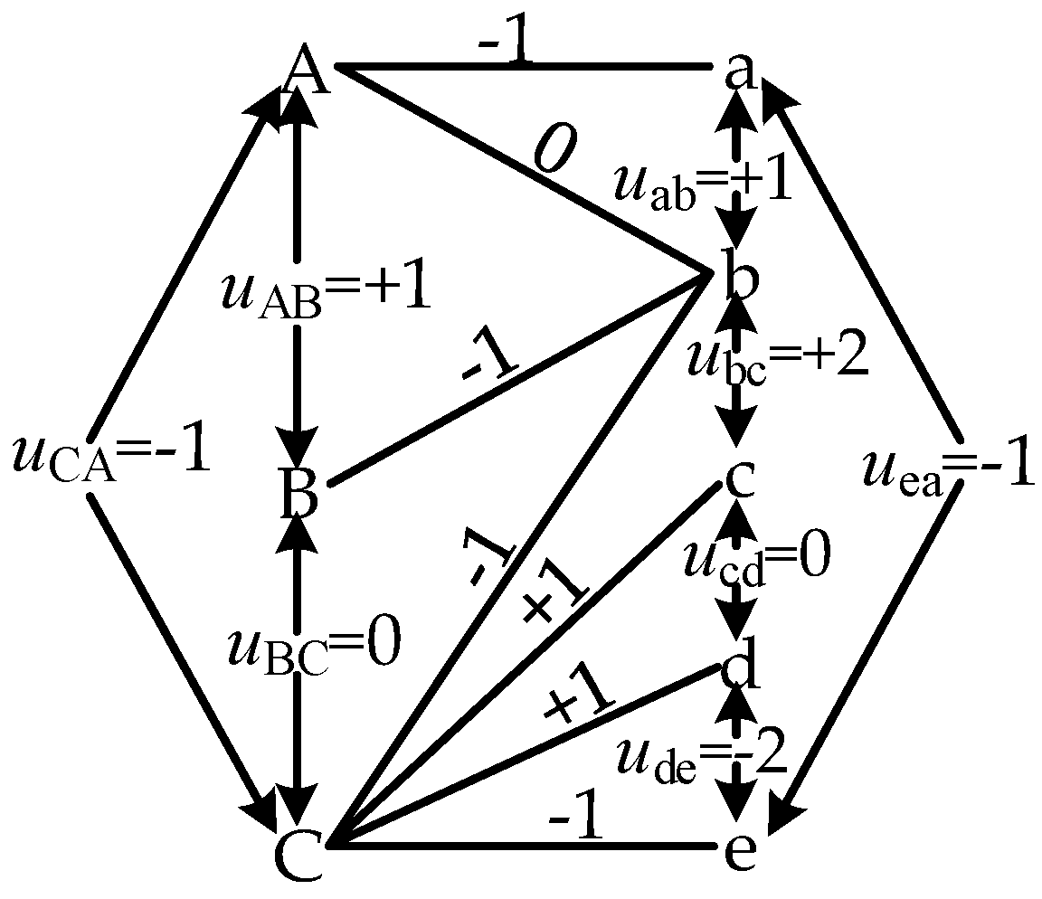
In contrast to the method used in three-phase M3C, the branch connection of all vector combinations in the five-phase M3C should be found independently, assuming that the requirements of the constraints are fulfilled, and some connection forms can only satisfy one kind of vector combination. Branch connection and the bridge voltage are shown in Figure 2 when the input side voltage is uAB = Ucap, uBC = 0, uCA = −Ucap, the output side voltage is uab = Ucap, ubc = 2Ucap, ucd = 0, ude = −2Ucap, uea = −Ucap.
In the process of synthesis, the sorting method is used to stabilize the capacitance voltage of each H-bridge cell. The charge and discharge state of each H-bridge cell is determined by the capacitance voltage of each unit in a branch and the direction of the bridge arm current. Thus, if the H-bridge cell has a relatively high voltage in discharge state, and the H-bridge cell has a low voltage in charge state, the capacitor voltage of each H-bridge cell can be well stabilized within a certain range.
3. Vector Synthesis and Time Calculation
Space Vector Pulse Width Modulation (SVPWM) is a simple and effective method to represent the magnitude and phase of three-phase voltage. This method is also suitable for 3 × 5 M3C modulation.
Switch combinations of 3 × 5 M3C can produce a total of 176 kinds of effective line-to-line voltage combinations, but only the vector which is in accordance with the trend of voltage changes can be used to synthesize the output voltages. Take two groups of vectors with the length 0.2906Ucap and 1.9919Ucap as an example, the two groups of vectors correspond to the same angles, V8 to V3, which correspond to the positive part of voltage uAB. The two trends are 0→−Ucap→+Ucap→+Ucap→−Ucap→0, 0→+Ucap→+2Ucap→+2Ucap→+Ucap→0. Clearly, the latter is more in line with the trend of a sine wave. By comparing different groups of vectors with different length, it can be found that, taking 10 vectors with length 1.9919Ucap and a zero vectors as basic vectors can realize the synthesis of five phase output voltages. This is transformed into the corresponding d-q coordinate value by Equation (1), as shown in Table 2.
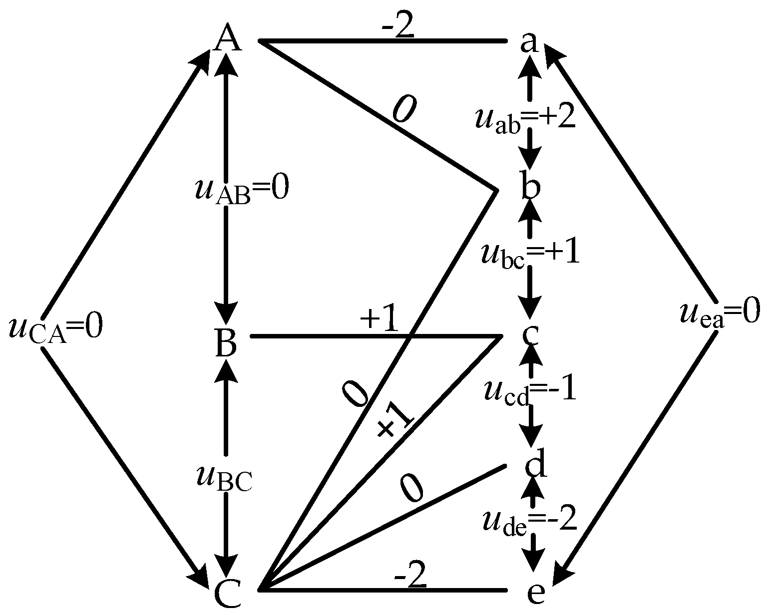
Based on the analysis of the structure and output voltage synthesis characteristics of the five phase M3C, it can be seen that the three-level synthesis method cannot synthesize five phase output voltage, and, thus, the output line voltage should have at least five levels. Therefore, when this group of models are adopted for synthesis, in the case of Vi0–Vo1~Vo10 vector combination, that is the input side is zero vector and the output side is Vo1 to Vo10, two of the three H-bridge cells are used for synthesis. Two effective branch states with +2Ucap, −2Ucap are added on the basis of three-level synthesis to satisfy the needs of the five-phase output. Take the Vi0–Vo1 vector combination as an example, the connection mode of the bridge and the states of each bridge are shown in Figure 3.
The situation of the branch is similar to + Ucap, −Ucap in the Vi0–Vo1~Vo10 vector combination case. The switch state is also selected by the sorting method when the output is +2Ucap or −2Ucap. The capacitor voltage states of the three H-bridge cells are measured, and two H-bridge cells are selected for output according to the bridge current direction and the H-bridge cells states. The output of +2Ucap, −2Ucap can solve the problem that three-level synthesis cannot synthesize five-phase output voltages.
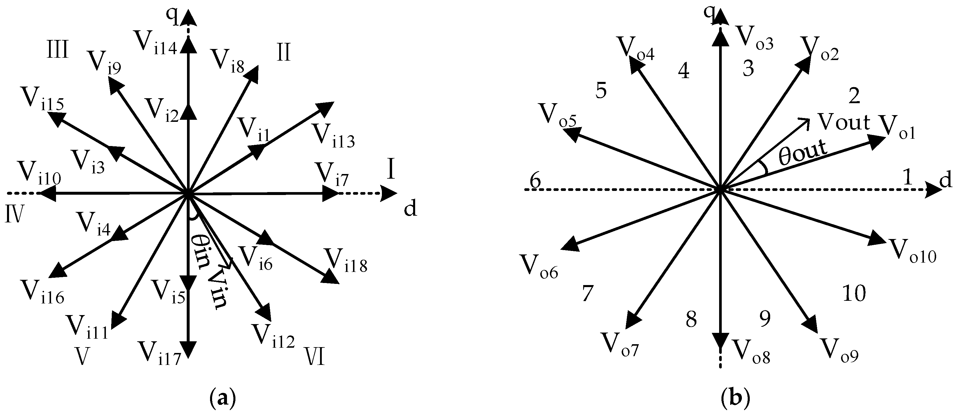
The input side is composed of 19 basic vectors, and the output side is composed of Vo0~Vo10. It can be seen from Table 2 that the amplitudes of Vo1~Vo10 are the same. The space vector figure at the input and output side is shown in Figure 4. Input and output are independent of one another. According to the mean equivalent principle, the given input/output reference vectors Vin and Vout are synthesized in one sampling period Ts. A 360° circle in the input side is divided into six sectors by the long vectors; the angle of each sector is 60°. A 360° circle on the output side is divided into ten sectors by the 10 basic vectors except for the zero vector; the angle of each sector is 36°. The synthesis method on the input side refers to the traditional three-phase synthesis method mentioned in [17], and the SVPWM method was adopted on the output side. Take the output side reference vector Vout, which is located in the sector 2 shown in Figure 4, as an example. It is synthesized by vectors Vo1, Vo2 and Vo0. The corresponding action times are to1, to2, to0, and their sum is the switching cycle Ts. It can be derived by the sine theorem as follows:
The vector action times are calculated as follows:
Where |Vo1| = |Vo2| = 1.9919Ucap, and the value of the modulation coefficient m is |Vout|/(1.1708Ucap). In the space vector modulation strategy, the basic vectors used for the synthesis are selected firstly according to the reference vector. Then the duty ratio of each switch combination is determined according to the duty ratio, and then the specific state of each switch and the maintenance time of each state are determined. An example is as follows: Ucap = 200 V, the input reference vector is located in the sector VI. (|Vin| = 90 V, θin = 20°) the vectors applied for combination are Vi5, Vi6, Vi0 respectively, and the corresponding time is ti5, ti6, ti0; the output vector is located in the sector 2, (|Vout| = 100 V, θout = 45°), the applied vectors are Vo0, Vo1, Vo2, and the corresponding action times are to0, to1, to2. The switch combination timing method in [17] was adopted. Equation (2) can be applied to the output side, the calculation results are as follows:
- ti0 = 0.4883Ts, ti5 = 0.3340Ts, ti6 = 0.1777Ts,
- to0 = 0.8389Ts, to1 = 0.0413Ts, to2 = 0.1198Ts
Based on the results obtained above, the corresponding switching unit state and the sustaining time can be obtained as shown in Figure 5.
4. Simulation and Experimental Analysis of 3 × 5 M3C
4.1. Simulation
A simulation model of 3 × 5 M3C was constructed based on Matlab/Simulink. Simulation parameters are shown in Table 3, and the simulation results are shown as Figure 6, Figure 7, Figure 8, Figure 9 and Figure 10.
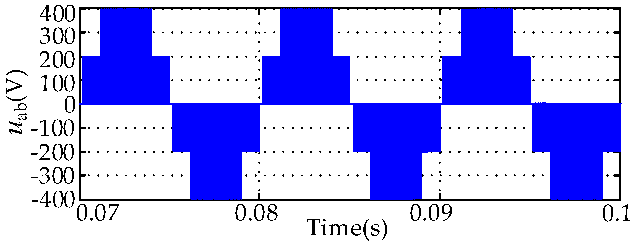
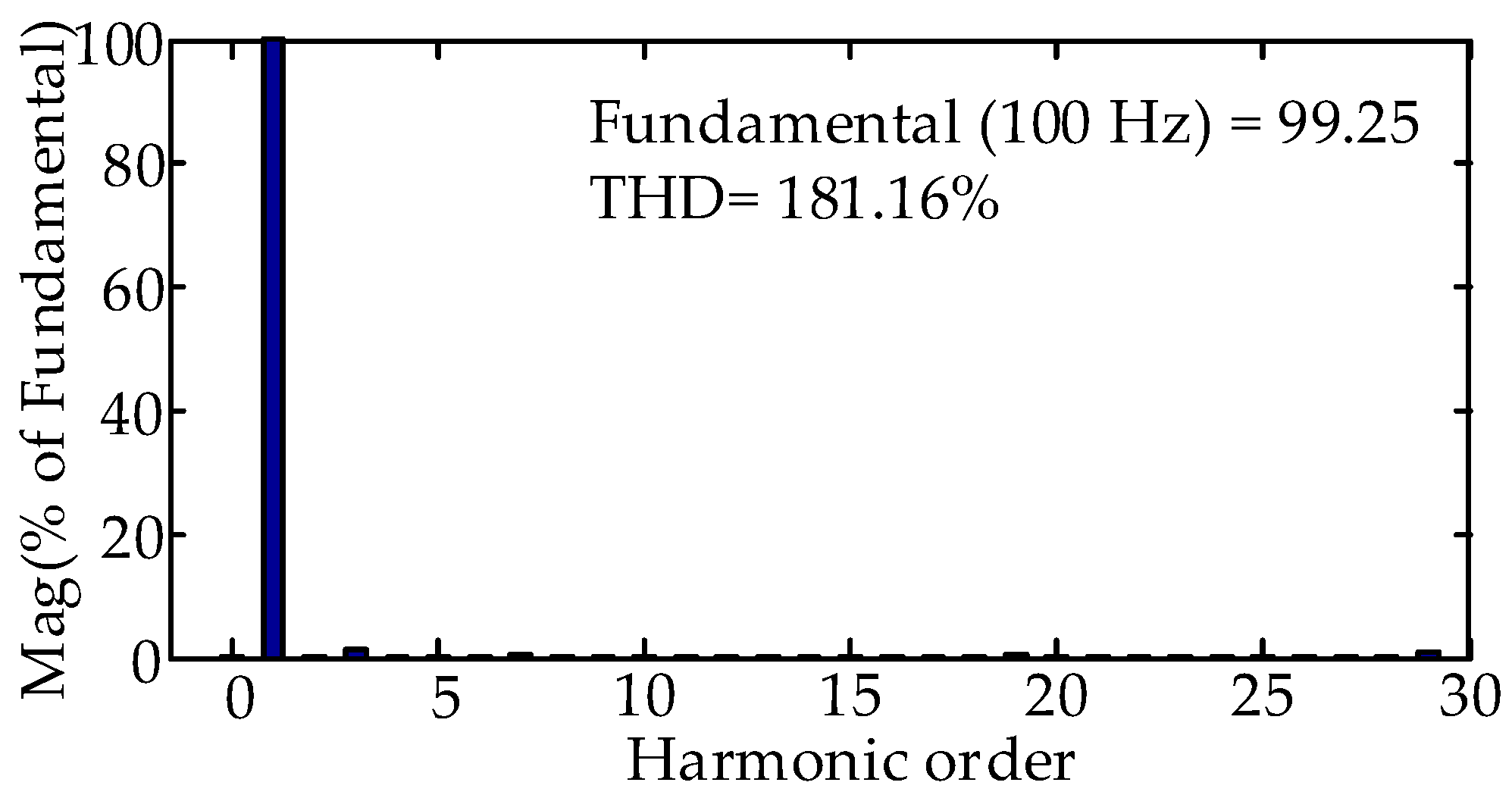
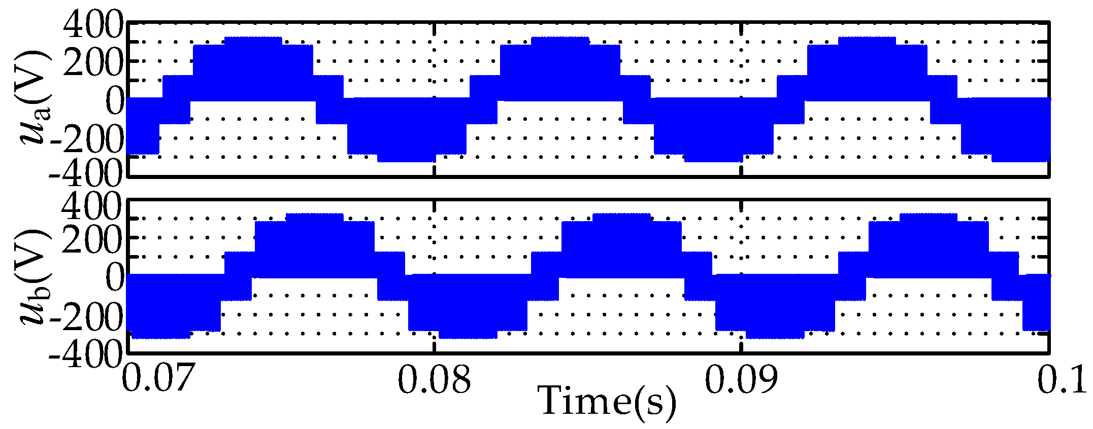
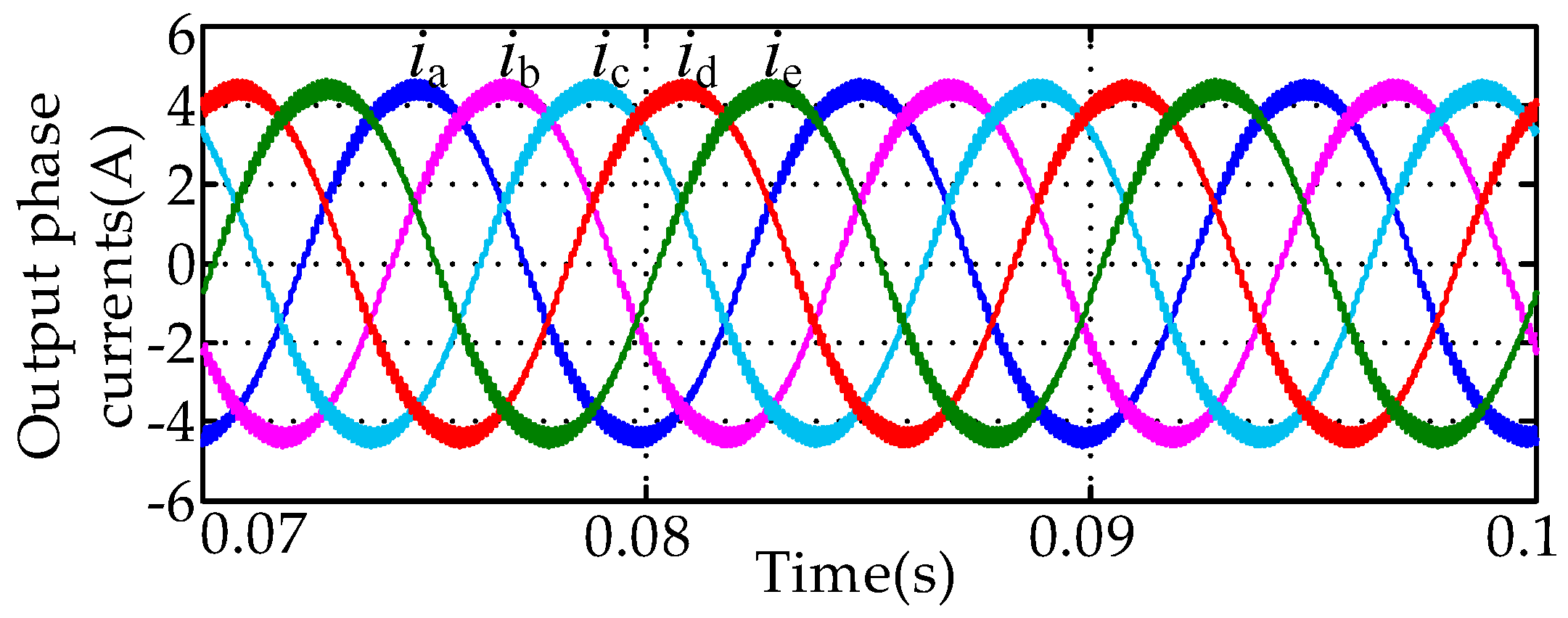
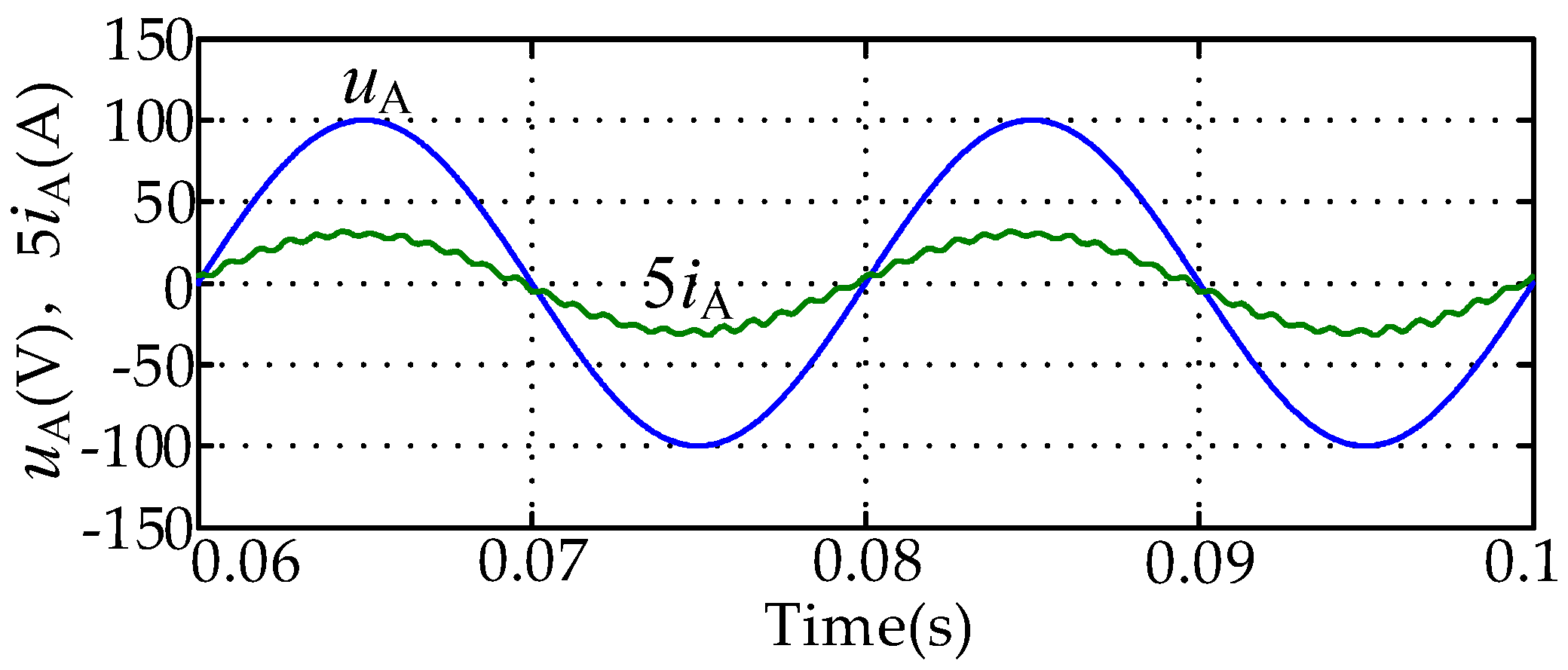
Capacitor voltage of H-bridge cell Ucap = 200 V. Different switching combinations can achieve five levels of line-to-line voltage. These 5 levels are: +400 V, +200 V, 0 V, −400 V, −200 V, respectively. As shown in Figure 6, the output line-to-line voltage uab contains five kinds of voltage levels: 0, ±Ucap, ±2Ucap. The spectrum analysis in Figure 7 shows that the fundamental amplitude of output line-to-line voltage is 99.25 V, which is close to the expected value of 100 V. The large THD values are mainly caused by high-order harmonics, and there are few low-order harmonics in the output voltage. The waveform of output phase voltages ua, ub are shown in Figure 8. It can be seen from this figure that the output phase voltage contains seven levels, and they are closer to the sine wave. Figure 9 shows the five-phase output currents waveform. They are symmetrical sine waves, which indicate good waveforms of output phase voltages. In Figure 10, the input current is in phase with the input voltage; thus, the unity power factor can be achieved.
4.2. Experiment
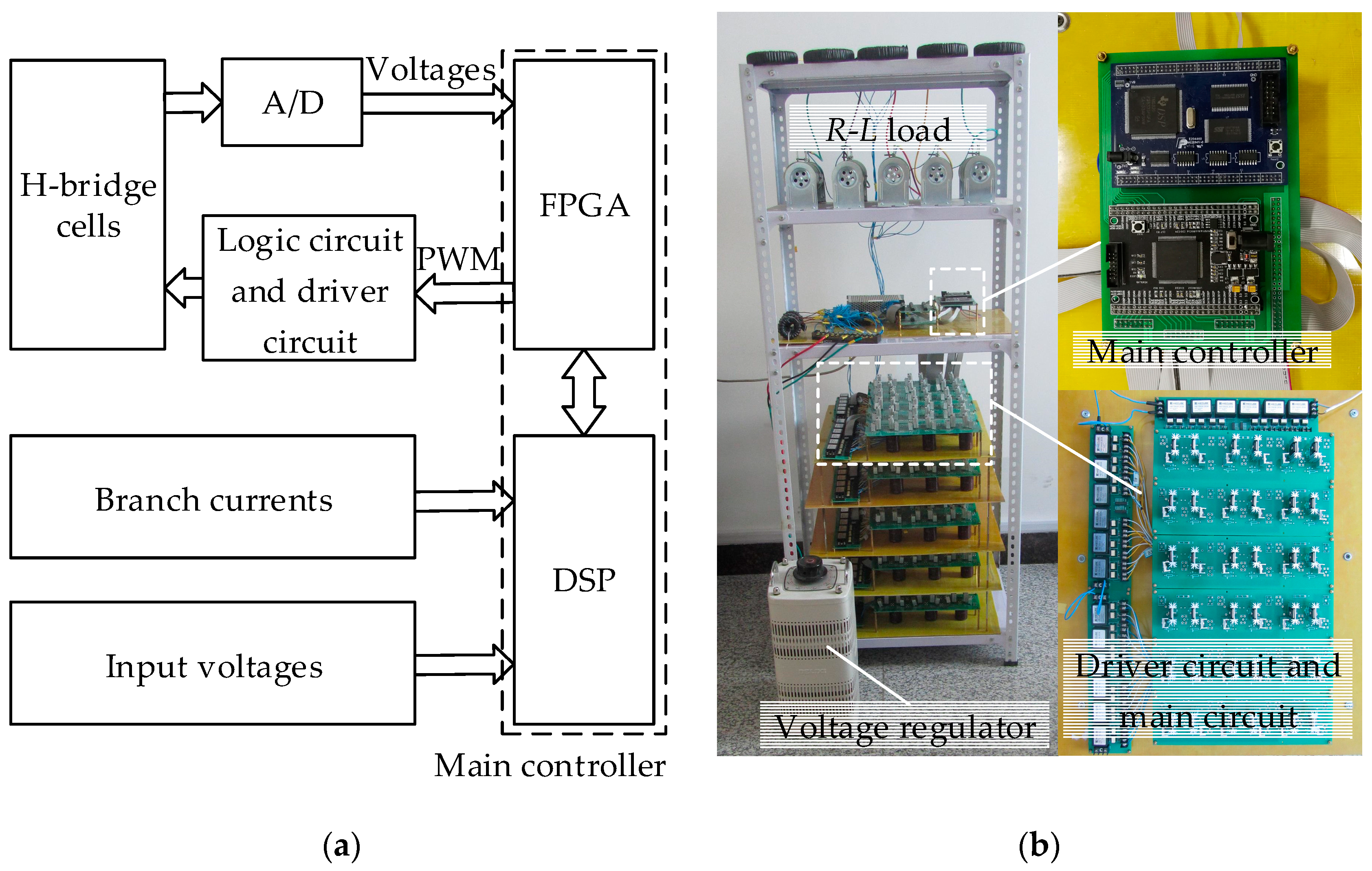
The configuration of our experimental platform is shown in Figure 11. The experimental platform is mainly composed of a three-phase power supply, main circuit, driver circuit, main controller, five-phase R-L load and some auxiliary circuits. The main circuit is mainly composed of MOSFET H-bridges. The optical coupler is employed in the driver circuit, and a logic circuit is integrated with it. The main controller includes a DSP and an FPGA chip. The segment division, duty cycle calculation and voltage sorting are completed by DSP. The FPGA is responsible for the generation of PWM signals and the configuration of A/D converter. According to the PWM signals, the logic circuit generates switching signals of MOSFETs in each H-bridge cell.
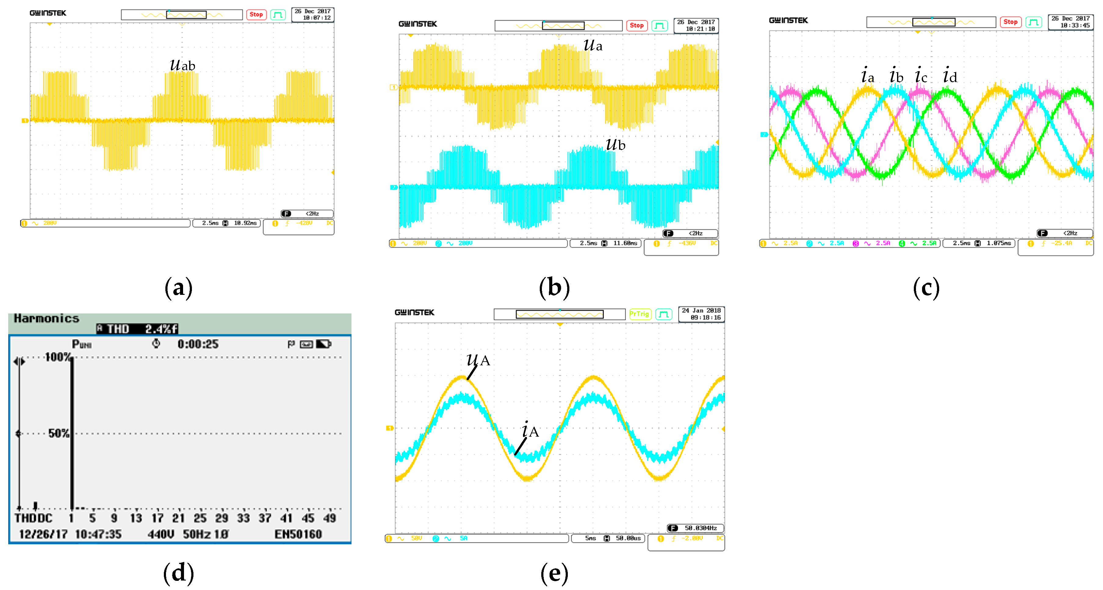
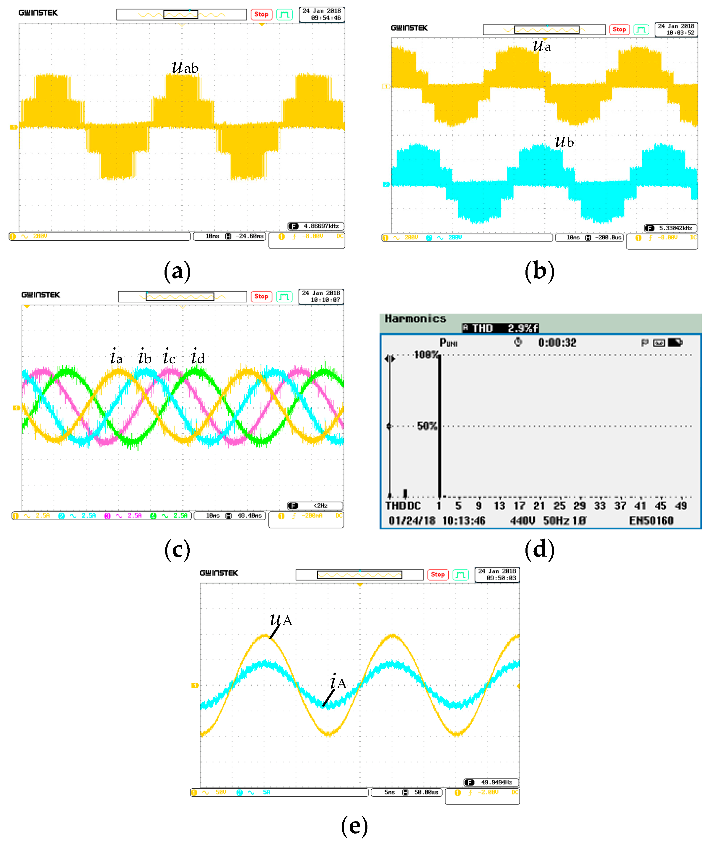
The experiment is divided into two cases. In the first case, the parameters are the same as in Table 3. In the other case, the parameters are the same except for the expected output line-to-line voltage, which is set to 80 V/25 Hz. The results of experiment are as follows.
Figure 12 is the experimental result of the first case. As can be seen from above, the output waveforms of the experiment are similar to that of the simulation. The output line-to-line voltage contains five voltage levels and the output phase voltage contains seven voltage levels. The output phase currents are sinusoidal and symmetrical, and the spectrum analysis of phase current in Figure 12d shows that there are little low-order harmonics. The value of THD is very low, which meets our expectations. The input current is nearly in phase with the input voltage, and the input power factor is close to unity power factor.
Figure 13 is the experimental result of the second case. The waveforms are similar to that of the first case, but the frequency and voltage magnitude has changed. The change of output voltage magnitude is indicated by the value of the output current. The output currents are still sinusoidal and symmetrical with little low-order harmonics. The phase of the input voltage and current are nearly the same. The output is able to follow the expected instruction.
The waveforms of this experiment are not very good compared with those of the simulation. The output voltages fluctuate near the expected voltage levels. This is mainly caused by the fluctuation of the capacitor voltage. The output current is not as smooth as that of the simulation. It mainly affected by the turn-on and turn-off delay of the switches and some disturbances. The input current is also affected by these factors. From the comparison, it can be seen that the shape and magnitude of the waveforms are very similar in Figure 6, Figure 8, Figure 9, Figure 10, and Figure 12. The difference of environment and devices between the experiment and the simulation makes the results slightly different. The results of the simulation and experiment all show that good performance is achieved in 3 × 5 M3C by the method proposed in this paper.
5. Conclusions
3 × 5 M3C is different from 3 × 3 M3C: an increased number of output phases, more H-bridge cells and more level voltages are needed for synthesis. This paper proposed a modulation strategy for 3 × 5 M3C. The segment division is very simple. Effective vectors are reasonably selected by this method. It is convenient to calculate the duty cycle, and the strategy can be implemented easily. The feasibility and validity of the proposed method were verified by means of computer simulation and experiment. It can be seen from the results of simulation and experiment that the expected five-phase output voltages are obtained. Desirable performance are achieved by this method. The method of adding branch states can also be expanded to other multiphase M3C.
Acknowledgments
This research is funded by National Key R&D Program of China under grant number 2017YFB0903300.
Author Contributions
Rutian Wang and Dapeng Lei conceived the theory; Yanfeng Zhao and Chuang Liu performed the experiments and analyzed the data; Yue Hu contributed materials and analysis tools; Rutian Wang and Dapeng Lei wrote the paper.
Conflicts of Interest
The authors declare no conflict of interest.
References
- Mengoni, M.; Zarri, L.; Tani, A.; Parsa, L.; Serra, G.; Casadei, D. High-torque-density control of multiphase induction motor drives operating over a wide speed range. IEEE Trans. Ind. Electron. 2015, 62, 814–825. [Google Scholar] [CrossRef]
- Jin, L.; Norrga, S.; Zhang, H.; Wallmark, O. Evaluation of a multiphase drive system in EV and HEV applications. In Proceedings of the 2015 IEEE International Electric Machines & Drives Conference (IEMDC), Coeur d’Alene, ID, USA, 10–13 May 2015; pp. 941–945. [Google Scholar] [CrossRef]
- Munim, W.N.W.A.; Che, H.S.; Hew, W.P. Fault tolerant capability of symmetrical multiphase machines under one open-circuit fault. In Proceedings of the IET International Conference on Clean Energy and Technology, Kuala Lumpur, Malaysia, 14–15 November 2016. [Google Scholar] [CrossRef]
- Bojoi, R.; Cavagnino, A.; Tenconi, A.; Tessarolo, A.; Vaschetto, S. Multiphase electrical machines and drives in the transportation electrification. In Proceedings of the 2015 IEEE 1st International Forum on Research and Technologies for Society and Industry Leveraging a Better Tomorrow (RTSI), Turin, Italy, 16–18 September 2015; pp. 205–212. [Google Scholar] [CrossRef]
- Baneira, F.; Doval-Gandoy, J.; Yepes, A.G.; López, Ó.; Pérez-Estévez, D. Control strategy for multiphase drives with minimum losses in the full torque operation range under single open-phase fault. IEEE Trans. Power Electron. 2017, 32, 6275–6285. [Google Scholar] [CrossRef]
- Levi, E.; Barrero, F.; Duran, M.J. Multiphase machines and drives—Revisited. IEEE Trans. Ind. Electron. 2016, 63, 429–432. [Google Scholar] [CrossRef]
- Mehrasa, M.; Pouresmaeil, E.; Akorede, M.F.; Zabihi, S.; Catalão, J.P.S. Function-based modulation control for modular multilevel converters under varying loading and parameters conditions. IET Gener. Transm. Distrib. 2017, 11, 3222–3230. [Google Scholar] [CrossRef]
- Mehrasa, M.; Pouresmaeil, E.; Taheri, S.; Vechiu, I.; Catalão, J.P.S. Novel Control Strategy for Modular Multilevel Converters Based on Differential Flatness Theory. IEEE J. Emerg. Sel. Top. Power Electron. 2017. [Google Scholar] [CrossRef]
- Mehrasa, M.; Pouresmaeil, E.; Zabihi, S.; Vechiu, I.; Catalão, J.P.S. A multi-loop control technique for the stable operation of modular multilevel converters in HVDC transmission systems. Int. J. Electr. Power Energy Syst. 2018, 194–207. [Google Scholar] [CrossRef]
- Wan, Y.; Liu, S.; Jiang, J. Integrated current-energy modeling and control for modular multilevel matrix converter. In Proceedings of the 2015 17th European Conference on Power Electronics and Applications (EPE’15 ECCE-Europe), Geneva, Switzerland, 8–10 September 2015; pp. 1–10. [Google Scholar] [CrossRef]
- Diaz, M.; Cardenas, R.; Espinoza, M.; Andrés Mora, F.R.; Clare, J.C.; Wheeler, P. Control of wind energy conversion systems based on the modular multilevel matrix converter. IEEE Trans. Ind. Electron. 2017, 64, 8799–8810. [Google Scholar] [CrossRef]
- Fan, B.; Wang, K.; Zheng, Z.; Xu, L.; Li, Y. Optimized branch current control of modular multilevel matrix converters under branch fault conditions. IEEE Trans. Power Electron. 2017. [Google Scholar] [CrossRef]
- Nademi, H.; Norum, L.E.; Soghomonian, Z.; Undeland, T. Low frequency operation of modular multilevel matrix converter using optimization-oriented predictive control scheme. In Proceedings of the 2016 IEEE 17th Workshop on Control and Modeling for Power Electronics (COMPEL), Trondheim, Norway, 27–30 June 2016; pp. 1–6. [Google Scholar] [CrossRef]
- Bessegato, L.; Norrga, S.; Ilves, K.; Harnefors, L. Control of modular multilevel matrix converters based on capacitor voltage estimation. In Proceedings of the 2016 IEEE 8th International Power Electronics and Motion Control Conference (IPEMC-ECCE Asia), Hefei, China, 22–26 May 2016; pp. 3447–3452. [Google Scholar] [CrossRef]
- Mora, A.; Espinoza, M.; Díaz, M.; Cárdenas, R. Model predictive control of modular multilevel matrix converter. In Proceedings of the 2015 IEEE 24th International Symposium on Industrial Electronics (ISIE), Buzios, Brazil, 3–5 June 2015; pp. 1074–1079. [Google Scholar] [CrossRef]
- Fan, B.; Wang, K.; Wheeler, P.; Gu, C.; Li, Y. A branch current reallocation based energy balancing strategy for the modular multilevel matrix monverter operating around equal frequency. IEEE Trans. Power Electron. 2018, 33, 1105–1117. [Google Scholar] [CrossRef]
- Erickson, R.; Angkititrakul, S.; Almazeedi, K. New Family of Multilevel Matrix Converters for Wind Power Applications: Final Report, July 2002–March 2006; National Renewable Energy Laboratory (NREL): Golden, CO, USA, 2006. [Google Scholar] [CrossRef]
Figure 1.
Main circuit topology of 3 × 5 M3C.

Figure 2.
Vector combination of Vi1–Vo2.

Figure 3.
Vector combination of Vi0–Vo1.

Figure 4.
Vectors of 3 × 5 M3C (a) Vectors of input side; (b) Vectors of output side.

Figure 5.
Timing of space vector.

Figure 6.
Output adjacent line-to-line voltage.

Figure 7.
Spectrum analysis of uab.

Figure 8.
Output phase voltages.

Figure 9.
Five-phase output currents.

Figure 10.
Input phase voltage and current.

Figure 11.
Configuration of experimental platform (a) system structure; (b) photos of experimental platform.
Figure 11.
Configuration of experimental platform (a) system structure; (b) photos of experimental platform.

Figure 12.
Experimental waveforms under the output parameter 100 V/100 Hz (a) output line-to-line voltage (uab); (b) output phase voltage (ua, ub); (c) output currents (ia, ib, ic, id); (d) the Fast Fourier Transformation (FFT) analysis of ia; (e) input phase voltage and current (uA, iA).
Figure 12.
Experimental waveforms under the output parameter 100 V/100 Hz (a) output line-to-line voltage (uab); (b) output phase voltage (ua, ub); (c) output currents (ia, ib, ic, id); (d) the Fast Fourier Transformation (FFT) analysis of ia; (e) input phase voltage and current (uA, iA).

Figure 13.
Experimental waveforms under the output parameter 80 V/25 Hz (a) output line-to-line voltage (uab); (b) output phase voltage (ua, ub); (c) output currents (ia, ib, ic, id); (d) the FFT analysis of ia; (e) input phase voltage and current (uA, iA).
Figure 13.
Experimental waveforms under the output parameter 80 V/25 Hz (a) output line-to-line voltage (uab); (b) output phase voltage (ua, ub); (c) output currents (ia, ib, ic, id); (d) the FFT analysis of ia; (e) input phase voltage and current (uA, iA).


Table 1.
Combination of all branch connections.
| A | B | C |
|---|---|---|
| 1 | 1 | 5 |
| 1 | 2 | 4 |
| 1 | 3 | 3 |
| 1 | 5 | 1 |
| 1 | 4 | 2 |
| 2 | 2 | 3 |
| 2 | 3 | 2 |
| 2 | 4 | 1 |
| 2 | 1 | 4 |
| 3 | 1 | 3 |
| 3 | 3 | 1 |
| 4 | 2 | 1 |
| 4 | 1 | 2 |
| 5 | 1 | 1 |
Table 2.
Vectors of output side.
| Five-Phase Voltage | Voltage in d-q Axis | Vector | |||||
|---|---|---|---|---|---|---|---|
| uab | ubc | ucd | ucd | ucd | ud | uq | |
| 2Ucap | Ucap | −Ucap | −2Ucap | 0 | 1.8944Ucap | 0.6155Ucap | Vo1 |
| Ucap | 2Ucap | 0 | −2Ucap | −Ucap | 1.1708Ucap | 1.6155Ucap | Vo2 |
| 0 | 2Ucap | Ucap | −Ucap | −2Ucap | 0 | 1.9919Ucap | Vo3 |
| −Ucap | Ucap | 2Ucap | 0 | −2Ucap | −1.1708Ucap | 1.6115Ucap | Vo4 |
| −2Ucap | 0 | 2Ucap | Ucap | −Ucap | −1.8944Ucap | 0.6115Ucap | Vo5 |
| −2Ucap | −Ucap | Ucap | 2Ucap | 0 | −1.8944Ucap | −0.6155Ucap | Vo6 |
| −Ucap | −2Ucap | 0 | 2Ucap | Ucap | −1.1708Ucap | −1.6115Ucap | Vo7 |
| 0 | −2Ucap | −Ucap | Ucap | 2Ucap | 0 | −1.9919Ucap | Vo8 |
| Ucap | −Ucap | −2Ucap | 0 | 2Ucap | 1.1708Ucap | −1.6115Ucap | Vo9 |
| 2Ucap | 0 | −2Ucap | −Ucap | Ucap | 1.8944Ucap | −0.6155Ucap | Vo10 |
| 0 | 0 | 0 | 0 | 0 | 0 | 0 | Vo0 |
Table 3.
Simulation parameters.
| Parameters | Value |
|---|---|
| Switching frequency | 5 kHz |
| Number of H-bridge cells in each branch | 3 |
| Capacitance of H-bridge cell | 1200 μF |
| Capacitor voltage | 200 V |
| Magnitude of input line voltage | 173 V |
| Input frequency | 50 Hz |
| Magnitude of output line voltage | 100 V |
| Output frequency | 100 Hz |
| Filter inductance in input and output side | 3 mH |
| Resistance of load | 16 Ω |
| Inductance of load | 12 mH |
© 2018 by the authors. Licensee MDPI, Basel, Switzerland. This article is an open access article distributed under the terms and conditions of the Creative Commons Attribution (CC BY) license (http://creativecommons.org/licenses/by/4.0/).
Share and Cite
MDPI and ACS Style
Wang, R.; Lei, D.; Zhao, Y.; Liu, C.; Hu, Y. Modulation Strategy of a 3 × 5 Modular Multilevel Matrix Converter. Energies 2018, 11, 464. https://doi.org/10.3390/en11020464
AMA Style
Wang R, Lei D, Zhao Y, Liu C, Hu Y. Modulation Strategy of a 3 × 5 Modular Multilevel Matrix Converter. Energies. 2018; 11(2):464. https://doi.org/10.3390/en11020464
Chicago/Turabian StyleWang, Rutian, Dapeng Lei, Yanfeng Zhao, Chuang Liu, and Yue Hu. 2018. "Modulation Strategy of a 3 × 5 Modular Multilevel Matrix Converter" Energies 11, no. 2: 464. https://doi.org/10.3390/en11020464
Note that from the first issue of 2016, this journal uses article numbers instead of page numbers. See further details here.