Multi-Rate and Parallel Electromagnetic Transient Simulation Considering Nonlinear Characteristics of a Power System

Abstract

The electromagnetic transient simulation of a power system with nonlinear characteristics is very time-consuming due to numerous inversion calculations of the admittance matrix. To speed up the simulation of the power system with nonlinear characteristics, a multi-rate and parallel electromagnetic transient simulation method is proposed. Firstly, a Multi-Area Thevenin Equivalents (MATE)-based parallel algorithm considering nonlinear characteristics of the power system is proposed. This method guarantees the admittance matrix is constant by considering changing branches as link current without dividing the subnet again. Secondly, considering the differences of the time constant of the AC/DC subnet, different simulation steps are used for these subnets. The Lagrange interpolation method is used for calculating the Thevenin voltage of the AC subnet in non-synchronous time. Calculation methods of the DC subnet Thevenin voltage is proposed by considering the simulation results during the entire large simulation step. Finally, the simulation process is optimized for improving the simulation efficiency further. The simulation results show that the proposed method could greatly improve the simulation efficiency without losing simulation accuracy too much compared with the traditional method.

1. Introduction

The electromagnetic transients program (EMTP) has been widely used for real-time simulation of power systems [1], verifying the control strategy [2], and detecting the operational status [3]. However, one of the limitations of conventional EMTP-type simulators is their inability of performing efficient simulations. The scale of power systems is expanding [4], and the efficiency of electromagnetic transient simulations cannot meet the needs of scientific tests and theoretical research.

The concept of “diakoptics” was first introduced by Kron in the 1950s [5]. Kron’s diakoptics was aimed at the solution of large power system networks with increased computational speeds. Jose.R.Marti proposed the MATE concept in order to solve the network in partitioned form [6]. The main philosophy of MATE is to split the solution of a large system into the solution of a number of smaller subsystems, plus the solution of the links joining the subsystems. Additionally, a multilevel MATE [7] and latency technique [8,9] are used in MATE, and these methods aim at simulating nonlinearities and solving the differential equations with different integration steps.

In essence, MATE, and its derivation algorithm, belong to the category of parallel computing. It has been proven that parallel computing techniques are very effective to accelerate power system simulations [10]. To enhance the parallelism of the simulations and reduce the time cost of synchronous operation for MATE, an implicit synchronization approach is proposed in [11]. A parallel multi-rate simulation algorithm based on network division through a transmission line is proposed in [12], and it possesses higher parallelized levels and efficiency than the implicit multi-rate algorithm. Advanced Digital Power System Simulator (ADPSS) integrated the node splitting algorithm [13] and partition/parallel method [14], and it could be used in electromagnetic transient simulations for AC/DC power systems with moderate scale.

In the process of electromagnetic transient simulation, inversion operation is the most time-consuming part of the whole simulation process. In recent years, the proportion of DC network, distributed power, and other elements with nonlinear characteristics are much more than ever before [15], and the nonlinear characteristics of power systems are getting stronger. These circumstances result in inversion operations needing to be repeated frequently in the simulation calculation, and must even be done in every step because of rapid switch events. This situation severely restricts the improvement of simulation efficiency. One solution is to remove the changing components when forming admittance matrices, and there are only constant components in the admittance matrices. Under the MATE-based parallel simulation architecture, those changing components could be treated as links between subnets in order to ensure the admittance matrix is constant during the entire simulation process. However, this method has the following problems: On the one hand, this network division method may result in an extremely uneven subnet scale. On the other hand, if there are too many changing components, the number of subnets will be too large. Both will result in extremely time-consuming synchronization operations.

Aiming at this problem, multilevel MATE is proposed in [7]. This method guarantees the admittance matrix is constant by eliminating branches with changing parameters, and this process is done in the subnet calculation unit. However, if the number of changing branches varies greatly from each other, the process of eliminating branches would affect the calculation equilibrium of each subnet. Additionally, the premise of eliminating branches is the subdivision of the subnet, therefore, it is inevitable to make some constant branches participate in this network division process, and the introduction of these branches would seriously affect the efficiency of eliminating changing branches.

In this paper, a multi-rate and parallel electromagnetic transient simulation method considering nonlinear characteristics of a power system is proposed, which aims at improving the simulation efficiency further. The key point of the proposed algorithm regards changing branches as links, but they are not used for network partitioning. This process is done in coordination with the calculation unit. This algorithm guarantees the admittance matrix remains constant during the entire simulation process, which is similar to multilevel MATE. The difference lies in that the proposed method does not need to make some constant branches participate in the network division process, and the calculation burden of these changing branches is less than multilevel MATE. Additionally, multi-rate simulation is applied to the above algorithm aiming at improving simulation efficiency further.

The rest of the paper is organized as follows: In Section 2, a MATE-based parallel algorithm considering nonlinear characteristics of the power system is described. The manner in which the multi-rate simulation is applied to the above parallel algorithm is described in Section 3. The simulation process of the multi-rate and parallel electromagnetic transient simulation algorithm and its optimization are described in Section 4. Performance test results are shown in Section 5. Conclusions are presented in Section 6.

2. MATE-Based Parallel Algorithm Considering Nonlinear Characteristics of a Power System

In this section, the fundamentals of the MATE-based parallel algorithm considering nonlinear characteristics of a power system is described, and the physical significance of the parallel algorithm is analyzed.

2.1. Fundamentals

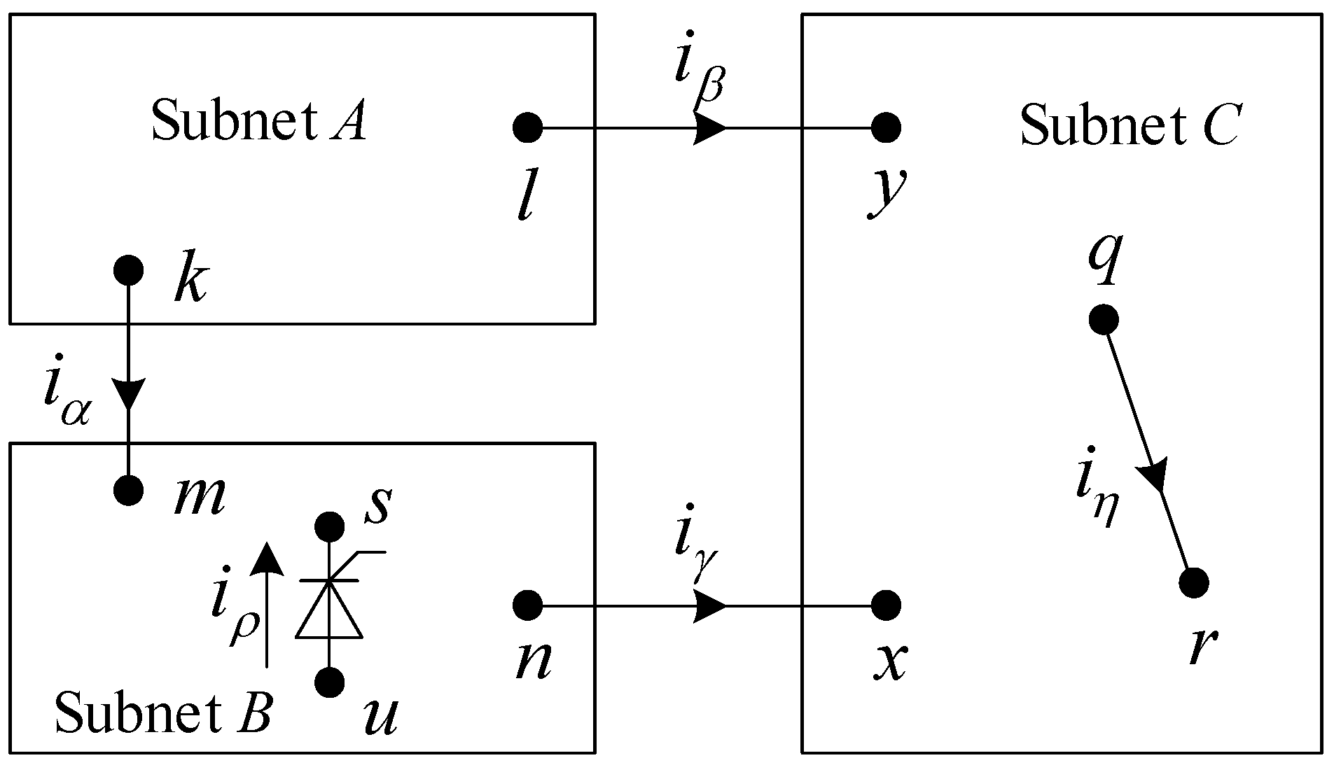
Taking an abstract AC/DC hybrid power system as an example, the parallel algorithm considering nonlinear characteristics of the power system is described. The partition of the sample power system is shown in Figure 1. Subnet B is a DC grid, including rectifiers, inverters, DC lines; the components in branch set s-u are switches, so the admittance matrix of subnet B is changing. Both subnet A and C are AC grids, and supposing the component parameters of subnet A are unchanging, which is changing in branch set q-r of subnet C under different operation states (such as an on-load tap changer, OLTC), the admittance matrix of subnet A is unchanging, which is opposite to that for subnet C.

It is worth noting that the node in Figure 1 does not specifically refer to a single node, but represents some node set, and we also suppose that “node set-node set” represents a branch set, such as l-y. In these branch sets, k-m, l-y, and n-x are used for network partitioning and are used to divide the network into different parts. s-u and q-r are the branch set with changing parameters, and they do not participate in the formation of admittance matrices.

The corresponding nodal equations of each subnet are as follows [6]:

$$G_A{V}_A+p_k{i}_{\alpha }+p_l{i}_{\beta }=h_A$$

(1)

$$G_B{V}_B+p_m{i}_{\alpha }+p_n{i}_{\gamma }+(p_s+p_u)i_{\rho }=h_B$$

(2)

$$G_C{V}_C+p_y{i}_{\beta }+p_x{i}_{\gamma }+(p_q+p_r)i_{\eta }=h_C$$

(3)

where G_i, V_i, and h_i denote the admittance matrix, node voltage, and accumulated current of subnet i (i denotes A, B, and C), separately. In particular, the elements of G_B and G_C don’t include s-u and q-r parameters, respectively. Therefore, G_A, G_B, and G_C are constant matrices. i_α, i_β, and i_γ denote the links’ current between subnets. i_ρ and i_η denote the links’ current of s-u and q-r. p_k, p_l, p_m, p_n, p_y, p_x, p_q, p_r, and p_u denote connectivity arrays, which reflect the relationship between the nodes and links’ current. In particular, let p_η denote p_q + p_r, p_ρ denote p_s + p_u.

As for s-u and q-r, the branch equations are:

$$p_{\rho }^T{V}_B=z_{\rho }{i}_{\rho }+e_{\rho }$$

(4)

$$p_{\eta }^T{V}_C=z_{\eta }{i}_{\eta }+e_{\eta }$$

(5)

where z_ρ, z_η, and e_ρ, e_η denote branch links’ Thevenin impedances and Thevenin voltages of s-u and q-r, separately.

From Equations (4) and (5), the dimension of i_ρ and i_η are proportional to the number of changing branches. In general, the number of these changing branches in the AC subnet is small and is uncertain for the DC subnet. For example, changing branches of twelve pulse rectifier circuits is much less than modular multilevel converter (MMC). As for the proposed method, the number of changing branches should not be too large, or the calculation amount of the links’ current would be extremely large.

As for k-m, l-y, and n-x, the branch equations are [6]:

$$p_k^T{V}_A+p_m^T{V}_B=z_{\alpha }{i}_{\alpha }+e_{\alpha }$$

(6)

$$p_l^T{V}_A+p_y^T{V}_C=z_{\beta }{i}_{\beta }+e_{\beta }$$

(7)

$$p_n^T{V}_B+p_x^T{V}_C=z_{\gamma }{i}_{\gamma }+e_{\gamma }$$

(8)

where z_α, z_β, z_γ, and e_α, e_β, e_γ denote the branch links’ Thevenin impedances and Thevenin voltagse of k-m, l-y, and n-x, separately.

By combining Equations (1)–(8), Equation (9) can be obtained:

$$\begin{array}{c}\left[\begin{array}{ccccc}{p}_k^T{G}_A^{-1}{p}_k+p_m^T{G}_B^{-1}{p}_m+z_{\alpha }& p_k^T{G}_A^{-1}{p}_l& p_m^T{G}_B^{-1}{p}_n& p_m^T{G}_B^{-1}{p}_{\rho }& 0\\ p_l^T{G}_A^{-1}{p}_k& p_l^T{G}_A^{-1}{p}_l+p_y^T{G}_C^{-1}{p}_y+z_{\beta }& p_y^T{G}_C^{-1}{p}_x& 0& p_y^T{G}_C^{-1}{p}_{\eta }\\ p_n^T{G}_B^{-1}{p}_m& p_x^T{G}_C^{-1}{p}_y& p_n^T{G}_B^{-1}{p}_n+p_x^T{G}_C^{-1}{p}_x+z_{\gamma }& p_n^T{G}_B^{-1}{p}_{\rho }& p_x^T{G}_C^{-1}{p}_{\eta }\\ p_{\rho }^T{G}_B^{-1}{p}_m& 0& p_{\rho }^T{G}_B^{-1}{p}_n& p_{\rho }^T{G}_B^{-1}{p}_{\rho }+z_{\rho }& 0\\ 0& p_{\eta }^T{G}_C^{-1}{p}_y& p_{\eta }^T{G}_C^{-1}{p}_x& 0& p_{\eta }^T{G}_C^{-1}{p}_{\eta }+z_{\eta }\end{array}\right]\\ \times \left[\begin{array}{c}{i}_{\alpha }\\ i_{\beta }\\ i_{\gamma }\\ i_{\rho }\\ i_{\eta }\end{array}\right]=\left[\begin{array}{c}{p}_k^T{G}_A^{-1}{h}_A+p_m^T{G}_B^{-1}{h}_B-e_{\alpha }\\ p_l^T{G}_A^{-1}{h}_A+p_y^T{G}_C^{-1}{h}_C-e_{\beta }\\ p_n^T{G}_B^{-1}{h}_B+p_x^T{G}_C^{-1}{h}_C-e_{\gamma }\\ p_{\rho }^T{G}_B^{-1}{h}_B-e_{\rho }\\ p_{\eta }^T{G}_C^{-1}{h}_C-e_{\eta }\end{array}\right]\end{array}$$

(9)

i_α, i_β, i_γ, i_ρ, and i_η could be obtained by solving Equation (9), and V_A, V_B, and V_C could be solved via putting them into Equations (1)–(3). From Equation (9), solving the inversion of the admittance matrix is inevitable when obtaining the links’ current. From above, G_A, G_B, and G_C are constant matrices, and their inversion is needed to be solved once during the entire simulation. Additionally, both links’ current of the changing and partition branches are solved together, which is different from the literature [7]. In [7], changing branches are dealt with in their subnet calculation unit.

2.2. Physical Significance of the Parallel Algorithm

In the electromagnetic transient parallel algorithm based on MATE, the power system is divided into several subnets. The influences among different subnets are reflected through the links’ current obtained by the Thevenin equivalent. The Thevenin equivalent regards some nodes as the research object, and acquires equivalent parameters in view of these nodes. Taking node k and l of subnet A as an example, the Thevenin voltage and impedance are described as follows:

In Equation (9), $p_k^T{G}_A^{-1}{h}_A$ and $p_l^T{G}_A^{-1}{h}_A$ denote the Thevenin voltages of nodes k and l, respectively. $p_k^T{G}_A^{-1}{p}_k$ and $p_l^T{G}_A^{-1}{p}_l$ denote the Thevenin self-impedance of nodes k and l, respectively. $p_k^T{G}_A^{-1}{p}_l$ and $p_l^T{G}_A^{-1}{p}_k$ denote the Thevenin mutual-impedance between node k and l.

3. Multi-Rate Simulation in Parallel Algorithm

In this section, the concept of non-synchronized time and synchronized time is described, and the way that multi-rate simulation is applied to the above parallel algorithm is described.

3.1. Concept of Non-Synchronized and Synchronized Time

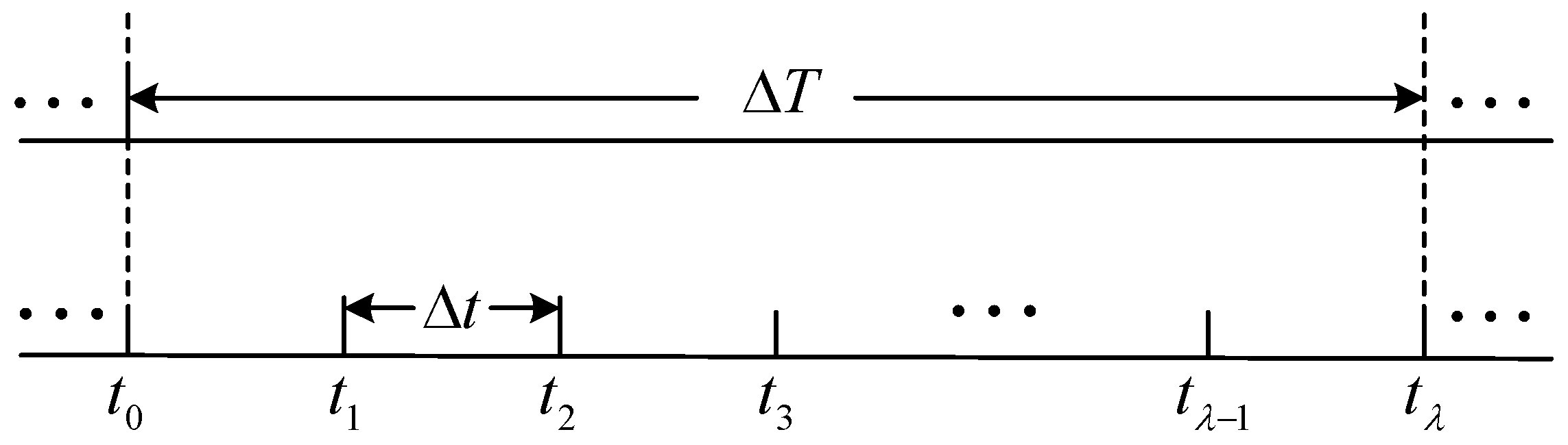
Supposing the simulation step of AC and DC subnets are $\Delta T$ and $\Delta t$, and $\Delta T=\lambda \Delta t$, in which $\lambda$ is an integer, the relationship of $\Delta T$ and $\Delta t$ is shown in Figure 2. During the entire $\Delta T$, only the DC subnet needs to be solved in t_i (i = 1, 2, …, λ − 1), which is called non-synchronized time. Both AC and DC subnets need to be solved in $t_{\lambda }$, which is called synchronized time. It is necessary to point out that $t_0$ in Figure 2 is the previous synchronized time.

In terms of network modeling, it is feasible to adopt different integral method. Common methods include the implicit trapezoidal integral method, Euler method, Gear integral method, and the Adams-Basfoss integral method. Considering the calculation amount and truncation error, this paper selects the implicit trapezoidal integral method to model the network.

3.2. Calculation Method at Non-Synchronized and Synchronized Time

Supposing the network is solved before $t_0$, the following text describes the calculation method in non-synchronized and synchronized time among a $\Delta T$.

3.2.1. Non-Synchronized Time

During non-synchronized time t_i (i = 1, 2, …, λ − 1), it is unnecessary and cannot calculate the Thevenin parameter of the AC subnet because of its simulation step $\Delta T$ ($\Delta T=\lambda \Delta t$). In spite of this, the AC subnet’s influence on the DC subnet exists during these periods, and it is obligatory to take this influence into consideration. In order to describe this influence, the paper uses Lagrange interpolate method to calculate Thevenin voltage of AC subnet.

As for AC subnet A or C, if its network solution of is solved at t₀, history current source at the next synchronized time t_λ of each element could be calculated according to the principle of electromagnetic transient simulation [16]. Then, the current source vector h_A(t_λ) and h_C(t_λ) could be formed. Additionally, the Thevenin voltage, in view of the link nodes, can be obtained, and the expression of them are shown in Equations (10) and (11):

$$E_{A\sim }(t_{\lambda })=p_{\sim }^T{G}_A^{-1}{h}_A(t_{\lambda })$$

(10)

$$E_{C\sim }(t_{\lambda })=p_{\sim }^T{G}_C^{-1}{h}_C(t_{\lambda })$$

(11)

where “~” denote node set k, l, x, y and branch set η. $E_{A\sim }$(t_λ) and $E_{C\sim }$(t_λ) denote the Thevenin voltage in view of “~” at subnets A and C, separately.

From above, the Thevenin voltage of subnets A and C at, and before, $t_0$ is known. Based on the Lagrange interpolation method, interpolation of the Thevenin voltage at any given moment can be obtained. Taking subnet A as an example, its interpolation Thevenin voltage is as follows:

$$E_{A\sim }(t)={\displaystyle \sum _{k=0}^K{\omega }_k(t)\cdot E_{A\sim }(t_{\lambda }-k\Delta T)}$$

(12)

where K + 1 denotes the number of interpolated nodes. ${\omega }_k(t)$ is the interpolated basis function which takes t as an independent variable, and $t_{\lambda }$, $t_{\lambda }-\Delta T$, …, $t_{\lambda }-k\Delta T$ as interpolated nodes. The Thevenin voltage of subnet A would be obtained when taking $t=t_1,t_2,\dots ,t_{\lambda -1}$ into Equation (12). The calculation for subnet C is completely identical to subnet A.

As for the DC subnet B, the history current source at t could be calculated using network solution at $t-\Delta t$, and then they are used to form $h_B$ at t. Then, the Thevenin voltage of subnet B could be calculated, whose expression is similar to Equations (10) and (11). This paper will not repeat them here.

Now, the Thevenin voltage of AC and DC at non-synchronized time have been calculated. Substituting them into the right of Equation (9), the links’ current could be calculated. Then take i_α, i_γ, and i_ρ into Equation (2), the subnet solution V_B can be calculated.

3.2.2. Synchronized Time

Both AC and DC subnets need to be solved in synchronized time $t_{\lambda }$. As for the AC subnet, its Thevenin voltage could be calculated using the last synchronized time; this part is already discussed in Section 3.2. However, as for the DC subnet, its network solution has been solved $\lambda -1$ times during the last $\Delta T$. Additionally, the topology of the DC subnet may have changed because of rapid switch events. Therefore, the influence of DC to AC could not be evaluated according to a certain non-synchronous simulation result of the DC subnet, and all the solution should be taken into account in order to improve simulation accuracy. Apparently, the traditional implicit trapezoidal integral method is not applicable because it only takes one calculation result to form the history source. Thus, the paper below takes an inductor in the DC subnet as an example, and illustrates its integral method.

The differential equation of inductor is shown as follows:

$$u_L=L\frac{d{i}_L}{dt}{u}_L=L\times \mathrm{d}{i}_L/\mathrm{d}t$$

(13)

We divide the interval $[t-\Delta T,t]$ into $\lambda$ sub-intervals with length $\Delta t$ and applying the traditional implicit trapezoidal integral method to Equation (13) with integral step $\Delta t$. Equation (14) can be obtained:

$$\{\begin{array}{c}\frac{u_L(t)+u_L(t-\Delta t)}{2}\Delta t=L{i}_L(t)-L{i}_L(t-\Delta t)\hfill \\ \frac{u_L(t-\Delta t)+u_L(t-2\Delta t)}{2}\Delta t=L{i}_L(t-\Delta t)-L{i}_L(t-2\Delta t)\hfill \\ ⋮\\ \frac{u_L(t-\Delta T+\Delta t)+u_L(t-\Delta T)}{2}\Delta t=L{i}_L(t-\Delta T+\Delta t)-L{i}_L(t-\Delta T)\hfill \end{array}$$

(14)

Substituting all the equations in Equation (14) together, Equation (15) can be obtained:

$$i_L(t)=\frac{u_L(t)}{R_L}+h_L^{\prime }(t)$$

(15)

where $R_L$ is the equivalent resistance of inductor, $h_L^{\prime }(t)$ is the history current source of inductor at synchronized time, the expression of both are as follows:

$$R_L=\frac{2L}{\Delta t}$$

(16)

$$h_L^{\prime }(t)=i_L(t-\Delta T)+\frac{u_L(t-\Delta T)}{R_L}+\frac{2}{R_L}{\displaystyle \sum _{k=1}^{\lambda -1}{u}_L(t-\Delta T+k\Delta t)}$$

(17)

Now, h_A, h_B, and h_C at synchronized time could be calculated. Inputting them into Equation (9), the links’ current could be calculated, then they are substituted for corresponding items in Equations (1)–(3) to calculate V_i (i denoting A, B, and C).

4. Simulation Process

In this section, the optimization of the algorithm is described. Then the simulation flowchart is shown to describe the simulation procedure.

4.1. Optimization of Simulation Process

The components in Equation (17) include the network solution in non-synchronized and synchronized time among the last $\Delta T$. The summation part of the history term in Equation (17) could be updated at the end of each small time step $\Delta t$, which avoids a large amount of calculation if all the addition tasks are executed when all the non-synchronized solutions have been obtained.

In addition, the process of calculating V_A, V_B and V_C is optimized. The Equations (1)–(3) are simply deformed and written in matrix form, and they are shown as follows:

$$\left[\begin{array}{c}{V}_A\\ V_B\\ V_C\end{array}\right]=\stackrel{firstitem}{\left[\begin{array}{c}{G}_A^{-1}{h}_A\\ G_B^{-1}{h}_B\\ G_C^{-1}{h}_C\end{array}\right]}-\stackrel{seconditem}{\left[\begin{array}{c}{G}_A^{-1}(p_k{i}_{\alpha }+p_l{i}_{\beta })\\ G_B^{-1}(p_m{i}_{\alpha }+p_n{i}_{\gamma }+p_{\rho }{i}_{\rho })\\ G_C^{-1}(p_y{i}_{\beta }+p_x{i}_{\gamma }+p_{\eta }{i}_{\eta })\end{array}\right]}$$

(18)

The first term $G_i^{-1}{V}_i$ on the right side of the Equation (18), could be calculated before the links’ current are obtained (i denote A, B, and C). Therefore, parallel calculations are used for solving $G_i^{-1}{V}_i$ and the links’ current. When the links’ current are solved, we substitute them into the second term on the right side of the Equation (18), and V_A, V_B, and V_C can be solved.

4.2. Simulation Process

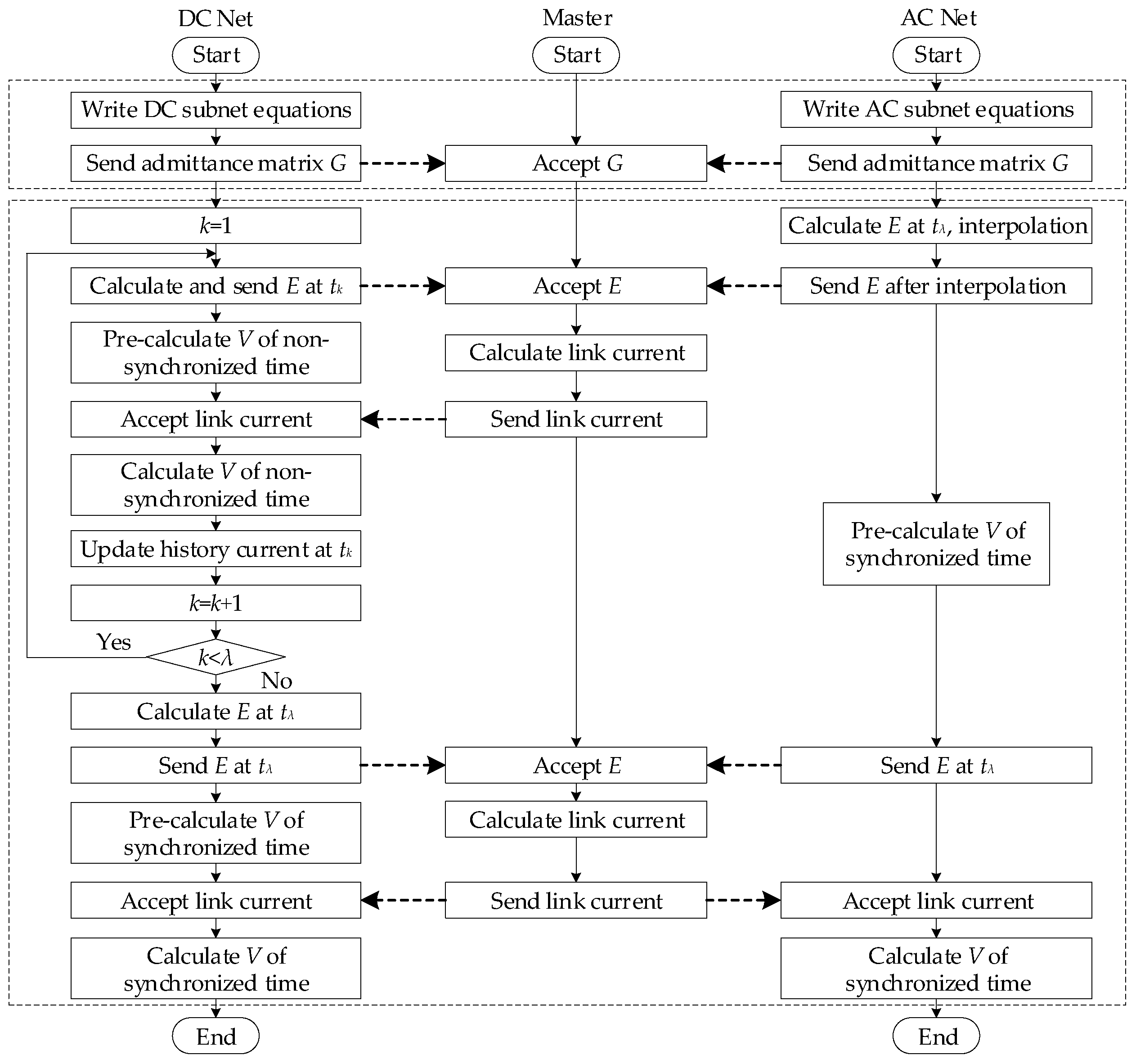
Figure 3 is the simulation process chart of this algorithm. The upper dashed box is the preprocess, which is mainly used for obtaining the admittance matrix and its inversion, and only needs to be calculated once in the whole simulation process. The lower dashed box is a simulation process among $\Delta T$, which is mainly used for pre-solution of the subnet network equation, acquiring the connection line current and the calculation of the node voltage. The calculation process of other $\Delta T$ is exactly the same as the lower dashed box.

In the upper dashed box, network equations of the DC and AC nets need to be written, and their admittance matrices are sent to the master side before simulation. Supposing the network has been solved before t₀, the calculation process of the lower dashed box is illustrated as follows:

(1)

For the AC subnet, calculate $E_{A\sim }(t_{\lambda })$ and $E_{C\sim }(t_{\lambda })$ based on the calculation results of t₀, which is shown in Equations (10) and (11), and interpolate to obtain their interpolation Thevenin voltage, which is shown in Equation (12).

(2)

For the DC subnet, let k = 1.

(3)

For the DC subnet, calculate $E_{B\sim }(t_k)$ based on the calculation results of $t_k-\Delta t$.

(4)

Send $E_{A\sim }(t_k)$, $E_{B\sim }(t_k)$, and $E_{C\sim }(t_k)$ to the master side, calculate the link currents according to Equation (9) and send them back to the DC net.

(5)

During procedure (4), $G_B^{-1}{h}_B(t_k-\Delta t)$ is calculated at the same time.

(6)

V_B is calculated according to the second line of Equation (18), and $h_B(t_k)$ is updated.

(7)

Let k = k + 1, and judge whether k < λ.

(8)

If k < λ, return to procedure (3). If not, go to procedure (9).

(9)

For the DC subnet, calculate $E_{B\sim }(t_{\lambda })$ based on the calculation results of the whole $\Delta T$.

(10)

During procedures (4) to (9), $G_A^{-1}{h}_A(t_0)$ and $G_C^{-1}{h}_C(t_0)$ are calculated at the same time, and $E_{A\sim }(t_{\lambda })$, $E_{C\sim }(t_{\lambda })$ could be obtained.

(11)

Send $E_{A\sim }(t_{\lambda })$, $E_{B\sim }(t_{\lambda })$ and $E_{C\sim }(t_{\lambda })$ to master side, calculate link currents according to Equation (9) and send them back to the AC and DC nets.

(12)

During procedure (11), $G_B^{-1}{h}_B(t_{\lambda }-\Delta t)$ is calculated at the same time.

(13)

V_A, V_B, and V_C are calculated according to Equation (18).

5. Simulation Results

In this section, the accuracy and efficiency analysis of the proposed algorithm is analyzed. The proposed method is achieved by programing in Matrix Laboratory (MATLAB).

5.1. Accuracy Analysis of Algorithm

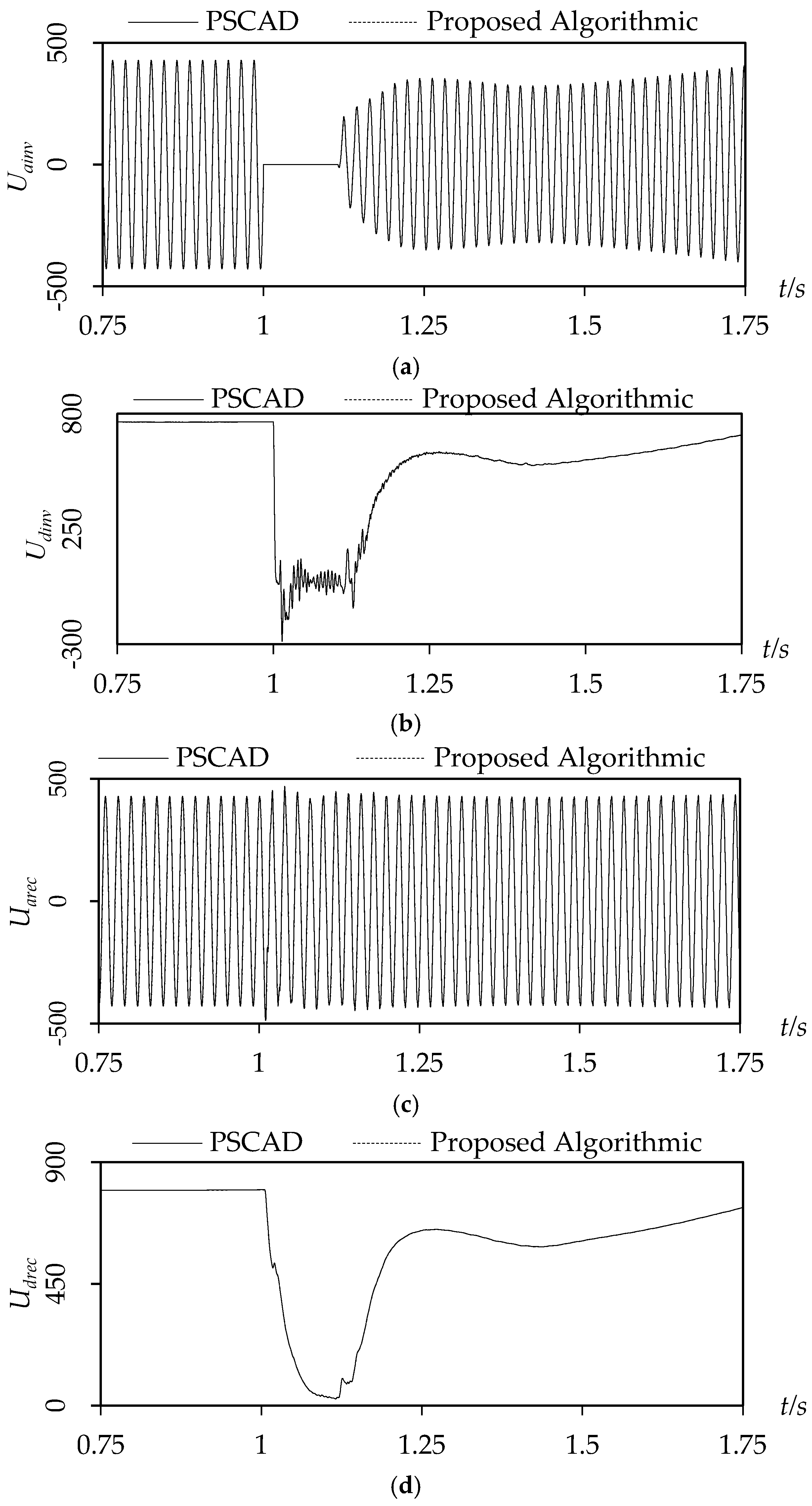
This paper uses an AC and DC hybrid system as the simulation example. The structure of this system is shown in Figure 4, and its parameters could be found in [17]. It is necessary to illustrate that the OLTC in Figure 4 is added by the author. The fault mode is that there is a three-phase metal to ground fault at the AC bus of the inverting side when the time is 1 s and lasts 100 ms.

In order to verify the accuracy of the proposed algorithm, the simulation result is compared with the results generated by PSCAD. The simulation step of PSCAD is 10 μs. The network needs to divide for this algorithm. This paper divides Figure 4 into three subnets, and each subnet is surrounded by a solid line. The simulation step for the AC sub-system is 50 μs, and is 10 μs for the DC sub-system. Additionally, the number of interpolated nodes is three and the integral method is the implicit trapezoidal integral method. The following paper would choose them as fundamental simulation settings if there are no additional instructions. Figure 5 shows the comparison of two simulation methods. In Figure 6, U_ainv is a phase voltage of the AC bus on the inverter side, U_dinv is the voltage of the DC bus on the inverter side, U_arec is the a phase voltage of the AC bus on the rectifier side, U_drec is the voltage of the DC bus on the rectifier side. From Figure 5, the simulation result of the proposed algorithm is in good agreement with that of PSCAD, and it proves the accuracy of the algorithm.

5.2. Analysis of Algorithm Efficiency

5.2.1. Influence of Subnet Partition on Efficiency

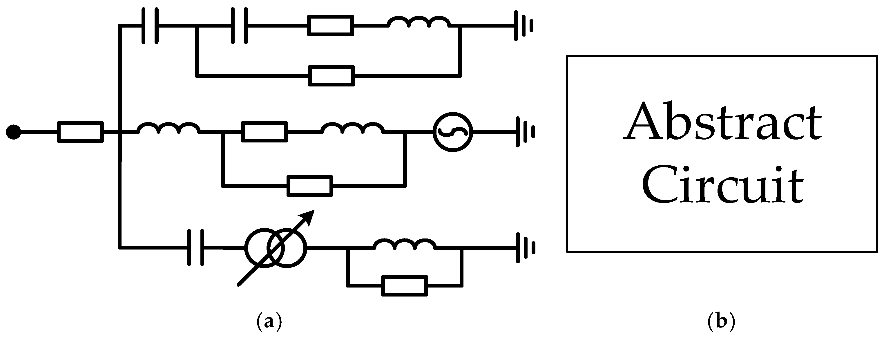
In order to verify the influence of subnet numbers on efficiency, the power system is divided in different ways. Apparently, the scale of the AC/DC hybrid system shown in Figure 4 is rather small and unnecessary to divide it further into more than three subnets. Therefore, the circuit shown in Figure 6a is added to Figure 4 in order to increase the node number, and Figure 6b is the abstract expression of Figure 6a. The system after processing is shown in Figure 7.

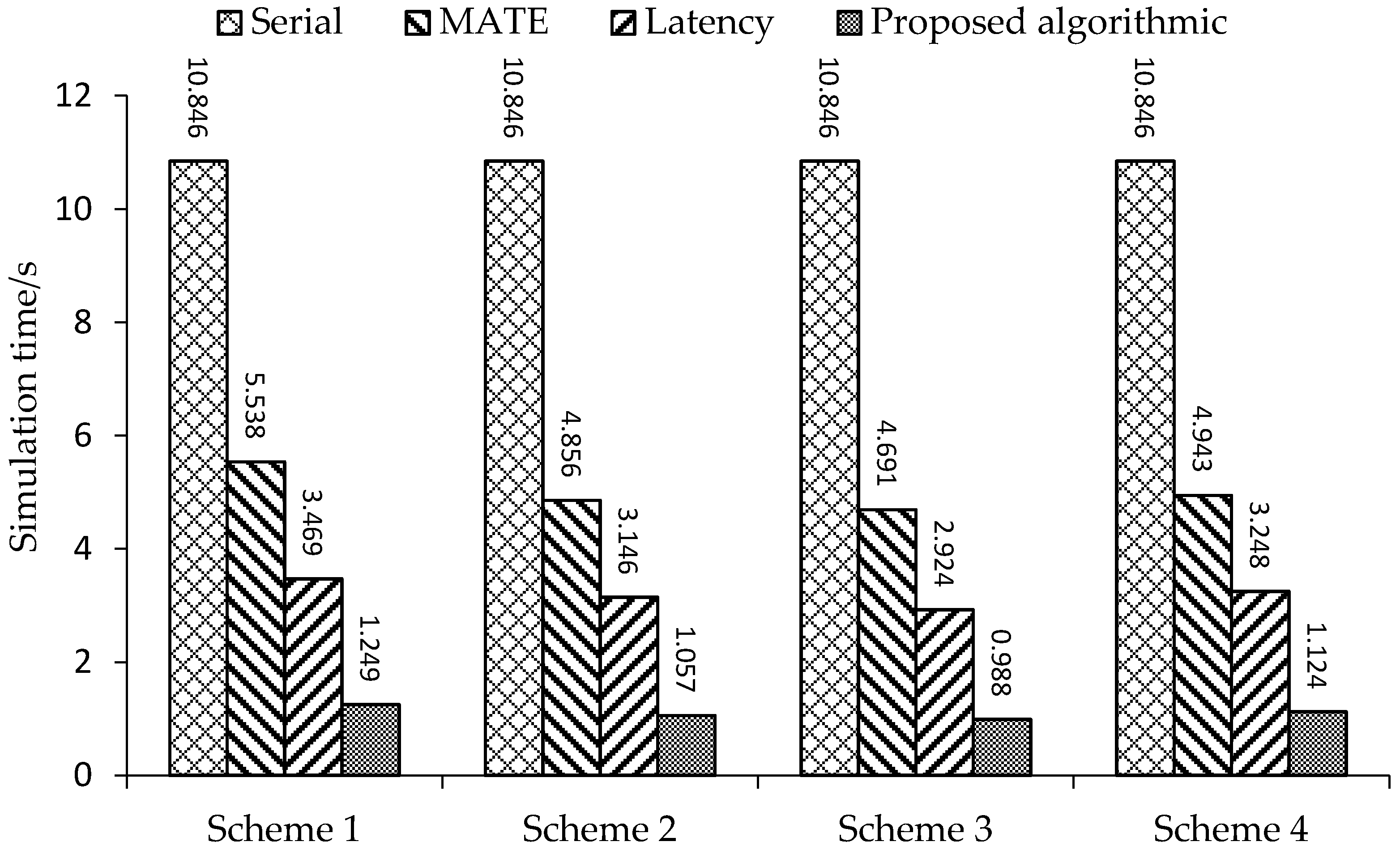
As for the power system in Figure 7, the partition principle lies in the scale of divided subnet is as uniform as possible, because it can decrease the synchronization waiting process. The system in Figure 7 is divided into fourteen areas, and different partition schemes are shown in

Table 1. Partition schemes.

Partition Scheme	Number of Subnets	Area Number
1	3	{1,2,3,4,5,6,8};{7};{9,10,11,12,13,14}
2	5	{1,2,3,8};{4,5,6};{7};{9,10,11},{12,13,14}
3	7	{1,2,8};{3,4};{5,6};{7};{9,10};{11,12};{13,14}
4	13	{1,8};{2};{3};{4};{5};{6};{7};{8};{9};{10};{11};{12};{13};{14}

. This paper compares the simulation time using the proposed algorithm with traditional serial, single-rate MATE parallel and multi-rate parallel methods based on latency simulation methods. The simulation time is 1 s, and the simulation step of these methods are shown in

Table 2. Setting of the simulation step.

Serial Number	Simulation Method	Simulation Step/μs
		AC Subnet	DC Subnet
1	Serial	10
2	MATE	10	10
3	Latency	50	10
4	Proposed algorithm	50	10

.

The simulation time under different partition schemes of these methods are shown in Figure 8. From Figure 8, the proposed algorithm could achieve the best simulation efficiency. Especially, the proposed algorithm could achieve real-time simulation in partition Scheme 3. Additionally, the three parallel simulation methods achieves their best simulation efficiency in this four-partition scheme, and it illustrates that Scheme 3 is a reasonable partition scheme and could distribute the calculation amount better among the subnets and the coordination calculation unit. In Scheme 3, the simulation rate of the proposed method is about eleven times that of the traditional serial simulation method. The reason lies in that, on the one hand, the admittance matrix of the proposed method is not influenced by the nonlinear elements with changeable characteristics; on the other hand, the multi-rate simulation is applied to the proposed method, and a faster simulation speed is achieved.

5.2.2. Influence of Subnet Scale on Efficiency

In order to verify the influence of subnet scale on efficiency, on the basis of Figure 4, this paper increases the nodes’ number by a paralleling circuit shown in Figure 6b on the AC bus. The system is simulated using methods in Section 5.2.1. Additionally, the AC networks on the inverter and rectifier sides are both divided into two parts with similar scales. In other word, the number of subnets is five for each method. The number of paralleled circuits on the AC bus and the simulation time of these methods are shown in

Table 3. Setting of simulation step.

Serial Number	Paralleled Circuit on AC Bus		Simulation Time/s
	Rectifier Side	Inverter Side	Serial	MATE	Latency	Proposed Method
1	1	1	6.742	4.084	2.881	1.156
2	5	5	10.846	5.538	3.469	1.249
3	10	10	16.485	7.963	4.615	1.439
4	15	15	23.617	10.864	7.544	1.813
5	20	20	35.554	15.694	12.437	2.126

. From Table 3, the simulation time of methods 1 to 3 increases rapidly with the expansion of the network scale, but for the proposed method, the network scale has a little impact on simulation time. The reason lies in that the admittance matrix in methods 1 to 3 is changeable, so the inverse operation must be applied to it at each simulation step. However, as for the proposed method, the elements with changeable characteristics do not participate in the formation of the admittance matrix, and the influence of these elements to the network is reflected in the injection current, which means that the inversion operation is just needed once for the admittance matrix during the entire simulation. Additionally, the method of this paper considers the time constant differences of the AC subnet and the DC subnet, and adopts the multi-rate simulation mode, so the simulation efficiency is better than the other methods.

5.2.3. Efficiency Comparison between the Proposed Method and Multilevel MATE

The method multilevel MATE parallel simulation algorithm, which is explained in [7], together with the proposed method could make the admittance matrix constant through a special operation. The difference lies in that multilevel MATE guarantees the admittance matrix is constant by eliminating the link current in the subnet, and belongs to single rate simulation. However, the proposed method guarantees the admittance matrix is constant by regarding changing branches as the link current, and belongs to the multi-rate simulation. In order to compare the efficiency of these two methods, the simulation step of the AC/DC subnets are set to be same, and the optimization of the calculation process is canceled for the method of this paper. The simulation time of these two methods for the systems in Section 5.2.2 is shown in

Table 4. Comparison of simulation time.

Serial Number	1	2	3	4	5
t1	2.048	2.216	2.587	2.896	3.465
t2	2.189	2.464	2.618	3.042	3.615
t2 − t1	0.148	0.248	0.031	0.146	0.150

, in which t₁ and t₂ represent the simulation time of the proposed method and multilevel MATE, respectively. In these two methods, each network is divided into three subnets, which is also the same as the partition scheme in Section 5.2.2.

The method of this paper deals with branches with changing parameters by assigning them to the link current calculation part. Multilevel MATE deals with branches with changing parameters by assigning them to the network equation solving part. From Table 4, the proposed method achieves better simulation efficiency at different network scales. The reason lies in the premise of eliminating the changing branches is the secondary subnet division as that for the multilevel MATE. However, in the process of the division, some branches with constant parameters are inevitably involved in the process of network secondary division, and the introduction of these branches will seriously affect the efficiency of eliminating branches. As for the method of this paper, it is just necessary to deal with the branches with changing parameters, and there is no need to divide the subnet again in this process, this illustrates that it does not need to involve constant branches into the calculation of the link current. Therefore, the proposed method is more efficient in the above examples. If the multi-rate simulation is applied in the above examples, the faster simulation speed will be achieved.

5.3. Influence of Algorithm Parameters

5.3.1. Number of Lagrange Interpolation Points

As for the AC network, this paper uses the Lagrange interpolation method to calculate Thevenin voltage of the AC subnet in non-synchronous time. Simulating the system of Figure 4 using different Lagrange interpolation points, and the average relative tolerance of the inverter DC bus voltage is shown in

Table 5. Average relative tolerance under different interpolation points.

Interpolation Point	2	3	4	5
Average relative tolerance	1.24%	1.08%	1.96%	3.19%

. The simulation settings are the same as Section 5.1 and the benchmark uses the PSCAD simulation results.

From Table 5, when the interpolation point is three, the average relative tolerance is the smallest. The reason may lie in that when the interpolation point is two, the interpolation polynomial is the result of two-point linear interpolation, and the interpolation point is not enough, which results in the interpolation polynomial being unable to reflect the dynamic characteristics of the power grid. When the interpolation point is greater than three (not including three), the structure of the interpolation polynomial is mainly influenced by the moment before the upcoming simulation, so it cannot reflect the dynamic characteristics of the upcoming simulation moment, too. Additionally, it will increase the amount of calculation.

In fact, the average relative tolerance of the proposed method is influenced by the grid structure, number of subnets, partition method, and simulation step. Apparently, an “interpolation point of three” behaves the best in this network under this simulation condition. The choice of the interpolation point number considering various factors is the future research focus.

5.3.2. Network Modeling Method

Simulating the network shown in Figure 4 using different integration methods, the average relative tolerance and simulation time under different methods are shown in

Table 6. Influence of the integral method on the simulation.

Integral Method	Average Relative Tolerance	Simulation Time
Implicit trapezoid	1.08%	1.057 s
Forward Euler	1.47%	1.044 s
Backward Euler	1.42%	1.046 s
Gear (2nd order)	1.19%	1.109 s
Adams-Bathurst (2nd order)	1.51%	1.124 s
Adams-Bathurss (3rd order)	1.49%	1.233 s

. The simulation settings are the same as Section 5.1 and the benchmark uses the Power Systems Computer Aided Design (PSCAD) simulation results.

From Table 6, the simulation efficiency is influenced slightly by different simulation methods. The implicit trapezoidal integration method obtained the highest simulation accuracy, and the second-order Gear integral method is slightly worse than the implicit trapezoidal integration method. The reason lies in that the truncation error of the two methods is proportional to the cubic of the simulation step, and the coefficient is smaller. As for other integration methods, the truncation error is proportional to the square of the simulation step, so the simulation precision is lower.

6. Conclusions

This paper presents a multi-rate and parallel electromagnetic transient simulation considering nonlinear characteristics of a power system. A parallel algorithm considering nonlinear characteristics of the AC/DC power system is introduced. On the basis of network division, this method regards branches with changing parameters as links and guarantees the admittance matrix is constant. Additionally, implementation of a multi-rate simulation in this algorithm is proposed.

(1)

The proposed method uses different simulation steps for subnets with different time constants. Compared with PSCAD, this method basically obtains exactly the same simulation result.

(2)

Under the same network partitioning conditions, the proposed method could achieve higher simulation efficiency compared with traditional serial, single-rate MATE parallel and multi-rate parallel methods, based on latency simulation methods.

(3)

The proposed method guarantees the admittance matrix is constant in the simulation process and avoids the repeated admittance inversion process. The efficiency of this method is slightly affected by the size of the network.

References

- Zhang, B.; Zhao, D.; Jin, Z.; Wu, Y. Multivalued Coefficient Prestorage and Block Parallel Method for Real-Time Simulation of Microgrid on FRTDS. Energies 2017, 10, 1248. [Google Scholar] [CrossRef]
- Song, S.; Kim, J.; Lee, J.; Jang, G. AC Transmission Emulation Control Strategies for the BTB VSC HVDC System in the Metropolitan Area of Seoul. Energies 2017, 10, 1143. [Google Scholar] [CrossRef]
- Qiu, W.; Huang, Y.; Zhang, X.; Xu, Z.; He, J. Test on electromagnetic transient in an operating UHVDC converter station. In Proceedings of the Advanced Research and Technology in Industry Applications, Ottawa, ON, Canada, 29–30 September 2014; pp. 1423–1425. [Google Scholar]
- Shao, S.J.; Agelidis, V.G. Review of DC System Technologies for Large Scale Integration of Wind Energy Systems with Electricity Grids. Energies 2010, 3, 1303–1319. [Google Scholar] [CrossRef]
- Kron, G. Tensorial Analysis of Integrated Transmission Systems; Part III. The “Primitive” Division. Trans. Am. Inst. Electr. Eng. Part III Power Appar. Syst. 1952, 71, 814–822. [Google Scholar]
- Martí, J.R.; Linares, L.R.; Hollman, J.A.; Moreira, F.A. OVNI: Integrated software/hardware solution for real-time simulation of large power systems. In Proceedings of the 14th Power Systerm Computation Confercence, Sevilla, Spain, 24–28 June 2002. [Google Scholar]
- Armstrong, M.; Marti, J.; Linares, L.; Kundur, P. Multilevel MATE for efficient simultaneous solution of control systems and nonlinearities in the OVNI simulator. IEEE Trans. Power Syst. 2006, 21, 1250–1259. [Google Scholar] [CrossRef]
- Moreira, F.A.; Marti, J.R. Latency techniques for time-domain power system transients simulation. IEEE Trans. Power Syst. 2005, 20, 246–253. [Google Scholar] [CrossRef]
- Moreira, F.A.; Mart, J.R.; Zanetta, L.C., Jr.; Linares, L.R. Multirate Simulations with Simultaneous-Solution Using Direct Integration Methods in a Partitioned Network Environment. IEEE Trans. Circuits Syst. I Regul. Pap. 2006, 53, 2765–2778. [Google Scholar] [CrossRef]
- Chen, L.; Chen, Y.; Xu, Y.; Ghong, Y. A novel algorithm for parallel electromagnetic transient simulation of power systems with switching events. In Proceedings of the International Conference on Power System Technology, Hangzhou, China, 24–28 October 2010; pp. 1–7. [Google Scholar]
- Chen, L.; Chen, Y.; Mei, S. An implicit synchro-nization approach and its application in parallel computation of electro-magnetic transient. Adv. Technol. Electr. Eng. Energy 2010, 29, 9–12. [Google Scholar]
- Mu, Q.; Li, Y.; Zhou, X.; Zhao, P.; Zhang, X. A Parallel Multi-rate Electromagnetic Transient Simulation Algorithm Based on Network Division Through Transmission Line. Autom. Electr. Power Syst. 2014, 38, 47–52. [Google Scholar]
- Yue, C.; Zhou, X.; Li, R. Study of parallel approaches to power system electromagnetic transient real-time simulation. Proc. CSEE 2004, 24, 1–7. [Google Scholar]
- Tian, F.; Zhou, X. Partition and Parallel Method for Digital Electromagnetic Transient Simulation of AC/DC Power System. Proc. CSEE 2011, 31, 1–7. [Google Scholar]
- Suh, J.; Hwang, S.; Jang, G. Development of a Transmission and Distribution Integrated Monitoring and Analysis System for High Distributed Generation Penetration. Energies 2017, 10, 1282. [Google Scholar] [CrossRef]
- Dommel, H.W.; Meyer, W.S. Computation of electromagnetic transients. Proc. IEEE 1974, 62, 983–993. [Google Scholar] [CrossRef]
- Arrillaga, J.; Watson, N. Power Systems Electromagnetic Transients Simulation; The Institution of Engineering and Technology: Hertfordshire, UK, 2003. [Google Scholar]
Figure 1.
Sample power system partition diagram.
Figure 2.
Relationship of and .
Figure 3.
Simulation flowchart.
Figure 4.
Standard test model.
Figure 5.
Comparison of the simulation results: (a) simulation comparison of Uainv; (b) simulation comparison of Udinv; (c) simulation comparison of Uarec; and (d) simulation comparison of Udrec.
Figure 6.
The circuit used to increase node of network: (a) actual circuit; and (b) abstract circuit.
Figure 7.
Test model after processing.
Figure 8.
Simulation time of different methods under different partition schemes.