Analysis of Switching Transients during Energization in Large Offshore Wind Farms
by
 ,
,
Gang Liu
1 ,
,
Yaxun Guo
1,*,
Yanli Xin
1,
Lei You
1,
Xiaofeng Jiang
1,
Ming Zheng
2 and
Wenhu Tang
1 1
School of Electric Power Engineering, South China University of Technology, Guangzhou 510640, China
2
Guangdong Electric Power Design Institute Co. Ltd. of China Energy Engineering Group, Guangzhou 510663, China
*
Author to whom correspondence should be addressed.
Energies 2018, 11(2), 470; https://doi.org/10.3390/en11020470
Submission received: 24 January 2018
/
Revised: 13 February 2018
/
Accepted: 19 February 2018
/
Published: 23 February 2018
(This article belongs to the Special Issue Emerging Power Electronics Technologies for Power Systems and Machine Drives)
Abstract
:In order to study switching transients in an offshore wind farm (OWF) collector system, we employ modeling methods of the main components in OWFs, including vacuum circuit breakers (VCBs), submarine cables, and wind turbine transformers (WTTs). In particular, a high frequency (HF) VCB model that reflects the prestrike characteristics of VCBs was developed. Moreover, a simplified experimental system of an OWF electric collection system was set up to verify the developed models, and a typical OWF medium voltage (MV) cable collection system was built in PSCAD/EMTDC based on the developed models. Finally, we investigated the influences of both the initial closing phase angle of VCBs and typical system operation scenarios on the amplitude and steepness of transient overvoltages (TOVs) at the high-voltage side of WTTs.
1. Introduction
Wind is an intermittent and random source of energy that causes vacuum circuit breakers (VCBs) to frequently switch wind turbine generators (WTGs), leading to a high possibility of switching overvoltages (SOVs) [1]. SOV, which exerts a significant impact on the insulation of electrical equipment in offshore wind farms (OWFs), is one of the main causes of transformer insulation failures. Therefore, it is necessary to study SOVs occurring in cable collection systems in OWFs, as this is important for the selection of appropriate protection measures and for the safety and reliability of OWFs.
There are already many studies that focus on SOVs of OWFs. The authors of [2,3,4] discussed the similarities and differences of transient overvoltages (TOVs) occurring in different systems, namely, OWFs, onshore wind farms, and industrial distribution systems; TOVs produced in medium voltage (MV) cable collecting systems of OWFs were also analyzed. An OWF experimental platform was set up in the laboratory [5,6,7], and, when prestrikes and reignitions occurred in VCBs, the measured overvoltage waveforms were used to establish simulation models that could reflect the electrical characteristics of VCBs and the high frequency (HF) characteristics of transformers. In [8], PSCAD/EMTDC and DigSILENT Power Factory were used to analyze the switching overvoltage in the MV cable collecting system of OWFs, and the simulation results were compared with measured data in an actual OWF. It was found that the simulation results can be improved greatly if an appropriate VCB model was included in PSCAD, whereas little improvement was found in DigSILENT. Based on the above discoveries, the authors of [9,10,11,12,13] used a PSCAD/EMTDC simulation to calculate TOVs when VCBs were operated in different configurations, and the results showed that TOVs were affected by many factors, such as the operating scenarios of OWFs, the transformer locations, the cable length, and the wave propagations in the cables.
However, these VCB models assumed a voltage level of 20 kV. The actual operating voltage level of a VCB is normally 35 kV. In addition, these studies mainly focused on overvoltage amplitude, and a quantitative analysis of overvoltage steepness was conducted. The quantitative analysis of overvoltage steepness is particularly important, because the inter-turn insulation of transformers is greatly affected by overvoltage steepness, and greater overvoltage steepness leads to greater stress imposed on the turn-to-turn insulation and a higher possibility of insulation failure.
Based on previous research, this paper mainly presents methods for HF models for submarine cables, wind turbine transformers (WTTs), and VCBs in PSCAD. In addition, an experimental system for a 35 kV electric collection system of an OWF was set up to verify the proposed models. Following this, the switching transient characteristics of the collection system of an OWF are studied using these models, and overvoltage steepness is quantitatively analyzed.
The rest of this paper is organized as follows: The following section presents the typical internal electrical system of an OWF and the modeling methodology of an OWF’s main components. Section 3 presents the model validation of the main components of an OWT. Section 4 analyzes the transient characteristics of overvoltages with different initial closing angles and system operation scenarios, and includes a quantitative analysis of overvoltage amplitude and steepness. Conclusions are drawn in Section 5.
2. Modeling of the Offshore Wind Farm
2.1. Layout Description of the Investigated Offshore Wind Farm
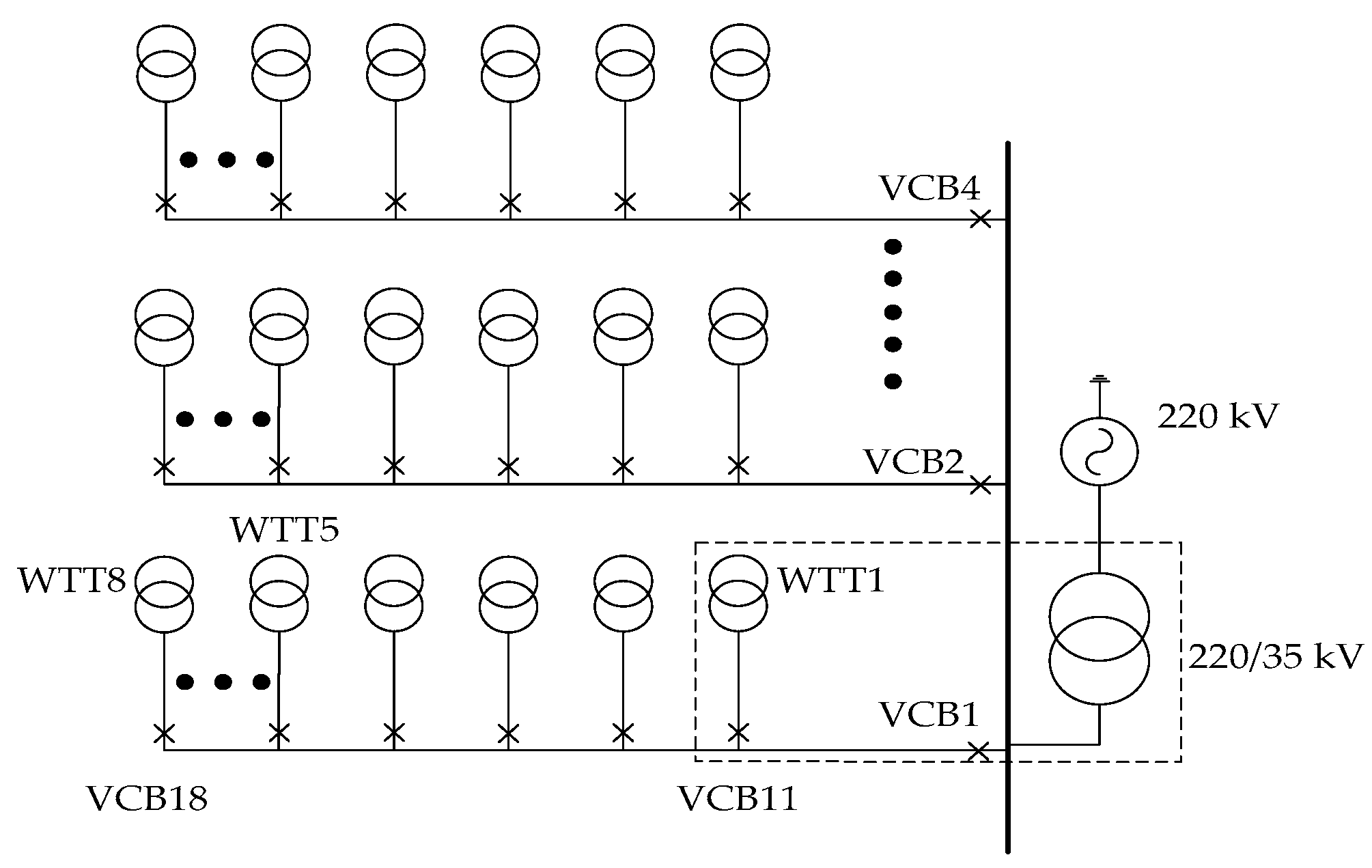
Figure 1 shows the single-side ring configuration of the investigated OWF, which consisted of 32 WTGs arranged in an array of 4 rows. WTGs were rated at 0.69 kV and connected to feeders by a 0.69/35 kV step-up transformer. The output voltage of the substation was raised to 220 kV, and the substation was connected to the external grid through submarine cables.
The length of the cable between each radial and the substation platform was 2 km. The distance between two neighboring wind turbines was 0.64 km. WTT1 was 0.08 km away from VCB11, and this distance is approximately equal to the height of a tower. Due to limitations of the laboratory arrangement, only a small section of the OWF was reproduced and is indicated by the dashed lines in Figure 1.
2.2. Modeling of Main Electrical Components
We mainly studied the SOVs of an MV collector system in an OWF; thus, the external grid is represented by a 220 kV ideal voltage source. Additionally, the 220 kV export cable from the substation platform is represented by a normal π model, while each 35 kV bus bar is represented by an ideal wire model. WTGs were not considered in this research.
In order to study the HF characteristics of SOVs, the HF characteristics of submarine cables, VCBs, and WTTs were fully considered, and these electrical components were modeled in PSCAD.
2.2.1. Modeling of Submarine Cables
Since the frequency-dependent (phase) model available in PSCAD/EMTDC (Manitoba HVDC Research Centre, Winnipeg, MB, Canada) can reflect the realistic electrical behaviors of submarine cables at various frequencies, especially the skin effects at HF, this model was used to model 35 kV submarine cables.
A three-core cable arrangement is depicted in Figure 2. The cable structure is simplified into four layers—Conductor, Insulation, Sheath, and Insulation—and the radius parameters of the layers are also shown. Since the armor layer of submarine cables is relatively thick, which prevents the flow of HF flux and thus prevents voltage loss, the armor is often assumed to be grounded [14]. Since the cable core conductor is composed of stranded conductors, a hollow conductor layer is utilized. In order to reduce the wave refraction of the transient surge and make it convenient for theoretical analysis, the parameters of all 35 kV submarine cables used in this study, including the cross section area (300 mm2), were the same; the cable parameters and installation conditions are summarized in Table 1 [15].
2.2.2. Modeling of Vacuum Circuit Breakers
Although operations of VCBs are random in nature, a deterministic model of a VCB was built to study the switching transients in different system operation scenarios. This is because a number of simulations with the same parameters are required to determine whether a scenario is potentially dangerous. Thus, the electrical parameters of VCBs (e.g., the dielectric withstand and the critical current derivative) are assumed to be constant in this study [16].
When contacts of a VCB close, the dielectric strength (DS) between contacts begins to decrease. When the transient recovery voltage (TRV) between contacts exceeds the DS, prestrikes occur. Prestrikes usually occur within the last few millimeters before contacts fully close, while the DS (Ub) between contacts approximates a linear decrease with closing time, as represented below [17]:
where TRVlimit is the maximum DS that a VCB can withstand, which is described by Equation (2); A is the rising rate of the DS, and B is the TRV of a VCB just before current zero crossing; t is the time; tclose is the moment when a breaker begins to close. According to [16] and the experimental results recorded in this study, A and B were set at 6.2 × 10⁷ V/s and 0, respectively.
where kaf is an amplitude factor; kpp is the first pole to clear factor; E_MAG is the rated voltage of a VCB.
Ub = TRVlimit − A(t − tclose) − B
When prestrikes occur, HF transient currents flow. The excellent interruption capability of VCBs promote the extinction of the arc at the current zero crossing, which is described by the value of di/dt at the current zero crossing. When di/dt is inferior to the critical value, VCBs interrupt HF currents; otherwise, the current continues to flow. The critical value is related to the VCB structure. Generally, it is between 100 and 600 A/μs [18]; in our study, we selected an average value (350 A/μs).
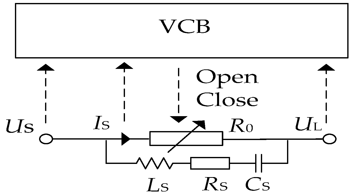
As shown in Figure 3, the VCB is equivalent to an ideal switch with parallel branches. The following parameters were used: RS = 50 Ω, LS = 50 nH, and CS = 200 pF [19]. The DS and HF current interrupting capabilities of VCBs were defined in a C language program in PSCAD. By detecting the VCB current (IS) and the voltage at both ends (US, UL), the controllable resistance, and the equivalent resistance of the VCB, R0 was changed in the program to simulate the opening and closing of the VCB.
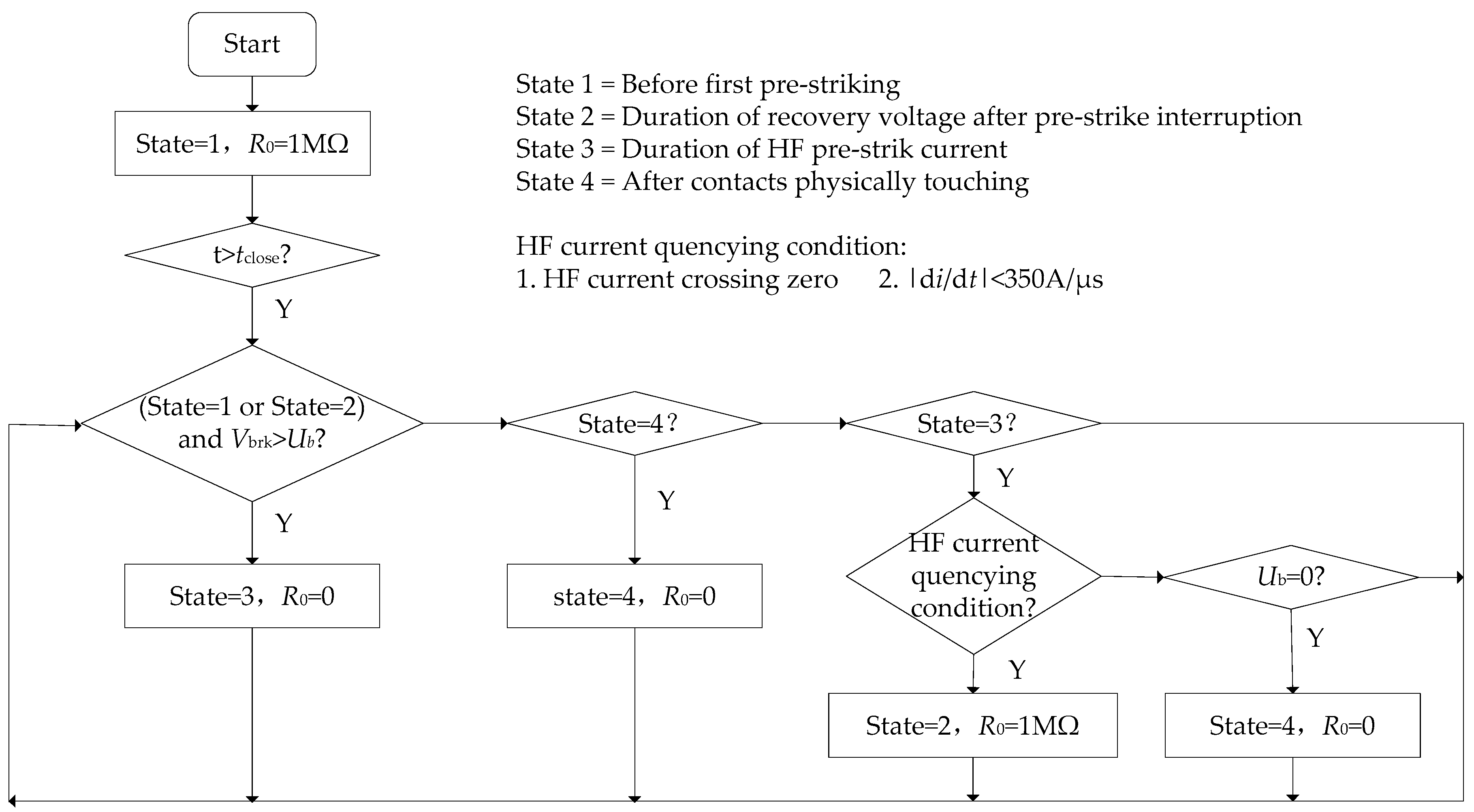
The program flow chart is shown in Figure 4. Before the VCBs receive the command to close and the first prestrikes occur, VCBs are all in State 1, and R0 is 1 MΩ. When the VCBs start to close, Ub decreases as the gap between contacts decreases. When the voltage difference across the VCB (Vbrk) exceeds Ub, prestrikes occur, the VCBs are in State 3, and R0 becomes zero. Afterwards, when the HF current crosses zero and di/dt is under the critical value, the VCBs turns off and are in State 2, and R0 is 1 MΩ. After this, the VCBs will experience State 2 and State 3 alternatively for a long time, until Ub decreases to zero and contacts of the VCBs are fully in contact—that is, when the VCBs fully close and are in State 4 and when R0 becomes zero.
2.2.3. Modeling of Transformers
In this study, the unified magnetic equivalent circuit (UMEC) model embedded in PSCAD was used to represent the substation transformers and WTTs. The UMEC model uses an I-V curve to simulate the nonlinear characteristics of an iron core, and it also takes into account the magnetic coupling relationships among three phases. The parameters of the substation transformers are given here as follows: rated capacity: 180 MVA; turns ratio: 220/35 kV; connection mode of winding: YNd11; equivalent leakage inductance: 0.06 per unit. For WTTs, these parameters are 5 MVA, 35/0.69 kV, Dyn11, and 0.02 per unit, respectively. Furthermore, parallel capacitances were added, including HV (high voltage)-ground capacitances, LV (low voltage)-ground capacitances, and HV-LV capacitance, which can reflect the HF characteristics of transformers [20]. The typical values of stray capacitances of transformers are shown in Table 2 [21].
3. Model Verification
Simulation models are usually verified through field measurements and laboratory experiments. Although field measurements are the best source of first-hand information, it is difficult to obtain all required information, and other factors regarding commerce and risk control should not be overlooked. Laboratory experiments refer to the building of experimental models in a laboratory, and the difficulty in such a method, in our case, lies in building an equivalent test system that reflects actual OWF operations. However, if a simulation model can be built, it then becomes easy to change components and test parameters to obtain data not readily available in field measurements. Therefore, in this study, simulation models were developed and verified with laboratory experiments.
In accordance with the part of Figure 1 marked with a dashed line, a test system was set up to verify the proposed model, as shown in Figure 5. The test system consisted of a VCB (40.5 kV), a transformer (TX1) (10/35 kV, 10 MVA), a transformer (TX2) (35/0.69 kV, 2 MVA), a reactor, a 150 kV high voltage probe (VD), a HF current transformer (TA) and cables. TX1 and TX2 represent the transformers located at the substation and WTT1 in Figure 1, respectively. Cable1 is the cable between VCB11 and VCB1 in Figure 1. Cable2 denotes the cable between VCB11 and WTT1 in Figure 1. The lengths of the two cables were 1 km and 0.08 km, respectively. Since the prestrike phenomenon is more obvious when VCBs close an inductive load [22], a reactor was adopted to represent an inductive load in the experimental platform; the reactor’s capacity was about 80% of TX2’s capacity. Due to the constraints of the experimental site, we only measured the voltage of Phase B at the high voltage side of TX2 and the current of Phase B at the load side of the VCB.
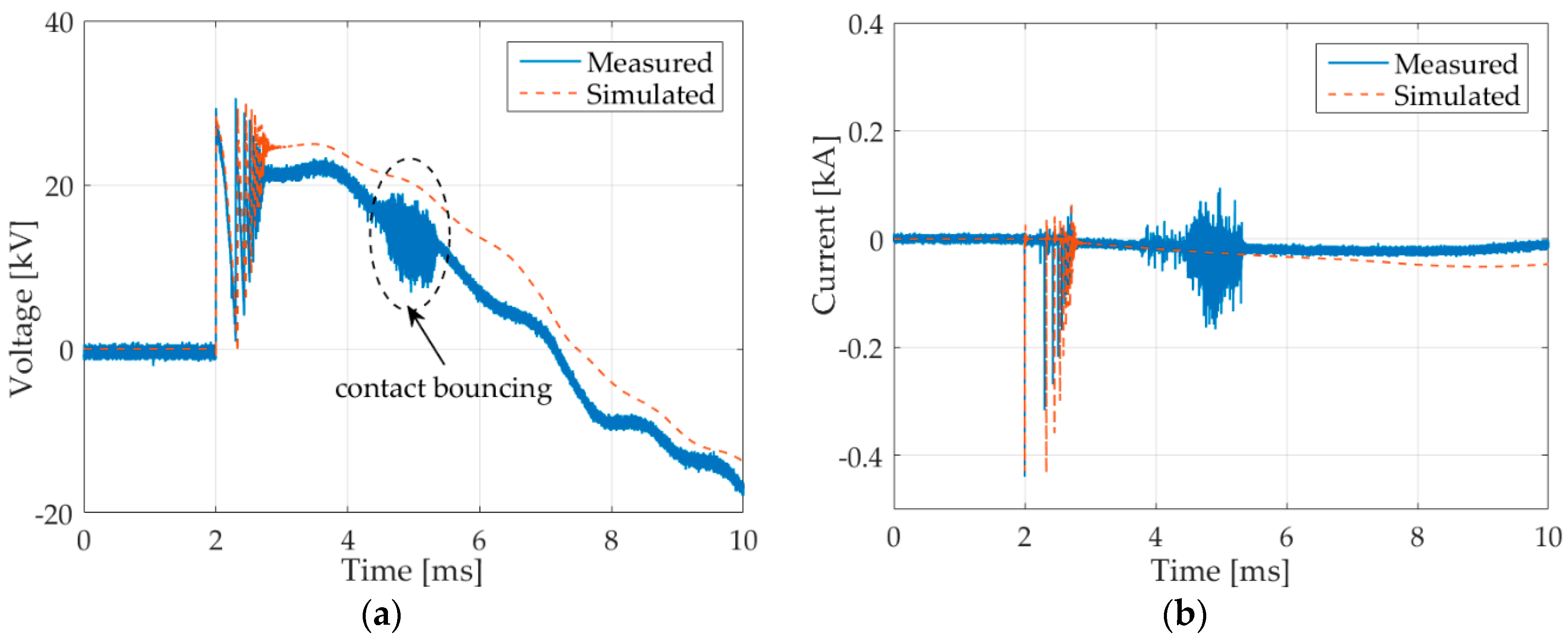
The experimental system shown in Figure 5 was also modeled in PSCAD based on the developed models in Section 2, and the simulation results obtained were compared with the experimental results in Figure 6. As shown in Figure 6, the first prestrike occurred at 2 ms and the second prestrike occurred at 2.3 ms, while the contacts of the VCB first made contact at 3.02 ms. However, the fluctuating amplitudes of the experimental waveforms were much larger than those of the simulated waveforms at the interval from 3.76 to 5.35 ms. This is because a rebound occurred when the contacts closed, and the gap between the contacts changed during the rebounding period, resulting in the variation of DS. However, such rebounding was not taken into account in the simulation model, and so the voltage fluctuation is not shown in the simulation results. This is because the period of rebounding is generally short, and the rebounding has little impact on the short circuit current making and on the breaking capabilities of the VCB [23].
The zoomed-in views of the measurement results for the first prestrike are shown in Figure 7. One can see that the fronts and amplitudes of the simulation waveforms are in good agreement with those of the experimental measurements, and this verifies the accuracy of the developed VCB model. Moreover, the times at which the measured and simulated voltages rise (a2, b2) occur slightly after the time at which the currents drops (a1, b1), and the time differences are very close to the propagation time of the waves in the cable; this illustrates the correctness of the wave impedance value in the cable model.
4. Simulation of High Frequency Overvoltage in Offshore Wind Farms
The amplitude and steepness of the TOVs are affected by many factors, including the initial closing angle and the operation modes of the VCBs [24,25]. The following VCB operation scenarios are considered in this study.
- (1)
- Scenario 1: closing a WTT when there is only one feeder in service, i.e., closing VCB11 when VCB1 has been closed, VCB12–VCB18 have all been closed, and VCB2–VCB4 have been opened.
- (2)
- Scenario 2: closing a feeder when all the VCBs connected to this feeder have been closed and all the other feeders are out of service, i.e., closing VCB1 when VCB11–VCB18 have been closed and VCB2–VCB4 have been opened.
- (3)
- Scenario 3: closing a feeder when all the VCBs connected to this feeder have been closed and some other feeders (the number is uncertain) are also in service, i.e., closing VCB1 when VCB11–VCB18 have been closed and VCB2 has also been closed.
4.1. Relationship between the Initial Closing Angle and Transient Overvoltages
When prestrikes occur, the steepness of TOVs at the high voltage side of WTTs is closely related to the current across the phase-ground capacitor, which is described in Equation (3).
where u is the voltage; i is the current flowing through the phase-ground capacitor; CH is the phase-ground capacitance.
The simulation results for Scenario 1 are shown in Figure 8. The overvoltage amplitude (1 p.u. = 28.58 kV) and the overvoltage steepness at the high voltage side of WTT1, along with the total number of three-phase prestrikes, all take 60° as a cycle; we also found that curves of these indicators are zigzagged. Additionally, for one angle cycle, the overvoltage amplitude and steepness rise and drop simultaneously. When the initial phase angle is 15°, the overvoltage amplitude (1.30 p.u.) and steepness (142 kV/μs), along with the total number of prestrikes (15), are the largest.
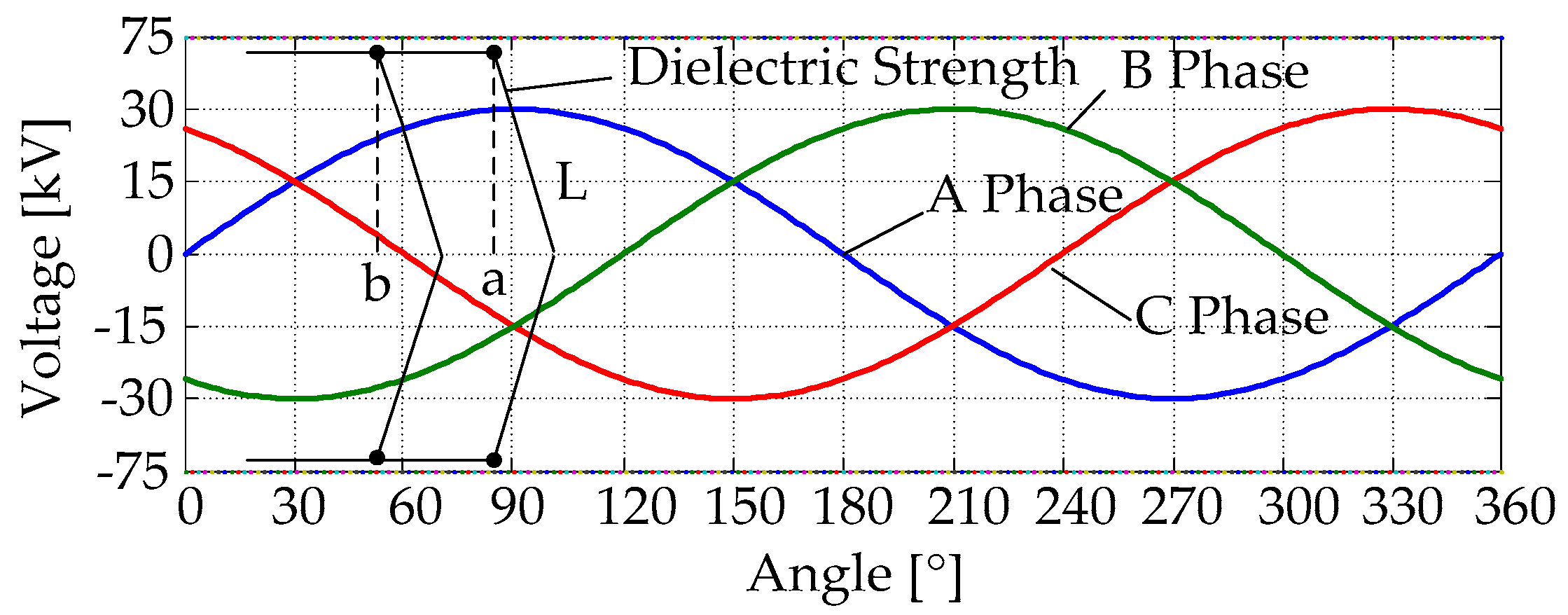
When the contacts of a VCB are closing, the TRV between the VCB contacts decrease due to the decreasing DS. A decreasing TRV leads to a decrease in the overvoltage amplitude and steepness at the high voltage side of the WTTs. Thus, when the first prestrike occurs at the peak voltage point, the TRV of VCBs is the largest, and the overvoltage amplitude and steepness are also the largest. This corresponds to the intersection between the DS curve L and the A phase voltage curve (at 90°) in Figure 9, and the angle of Point a becomes the initial closing angle; according to Equation (1) and the TRV curve of the VCBs, it is about 75°.
When the DS curve moves along the horizontal axis toward the negative semi-axis, the TRV value of the intersection, which is equal to the TRV when the first prestrike occurs, decreases continuously. Additionally, when the DS curve intersects with the A phase curve at 60°, the TRV value is at its lowest, thus producing the lowest overvoltage amplitude and steepness. Furthermore, the angle of point becomes the initial closing angle: about 45°.
Therefore, as for the A phase, the range of the initial closing angle, which corresponds to the first prestrike, is from 45° to 105°, that is, the overvoltage amplitude and steepness show a cycle of 60°, which is in good agreement with the simulation results in Figure 8.
4.2. Relationship between Transformer Location and Overvoltage
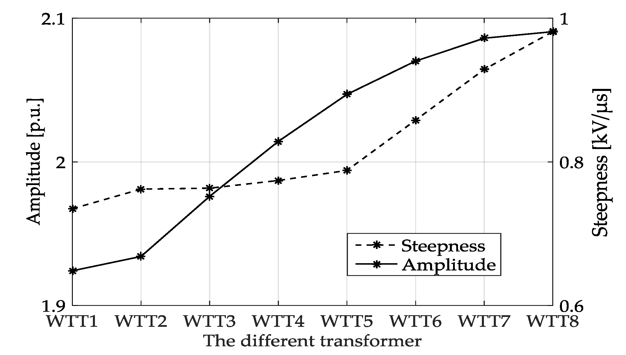
The simulation results for Scenarios 2 and 3 are shown in Figure 10 and Figure 11, respectively. For Scenario 2, the overvoltage amplitude and steepness increase as the distance from the bus increases. For Scenario 3, the overvoltage amplitude increases as the distance from the bus increases, but the opposite is true for the steepness, except for WTT7 and WTT8. This is because in Figure 11b, the steepness of TOV at the high side of WTT8 is higher than that of WTT7; that is, the steepness rises at the end of the feeder.
4.3. The Relationship between the Number of Running Feeders and Overvoltages
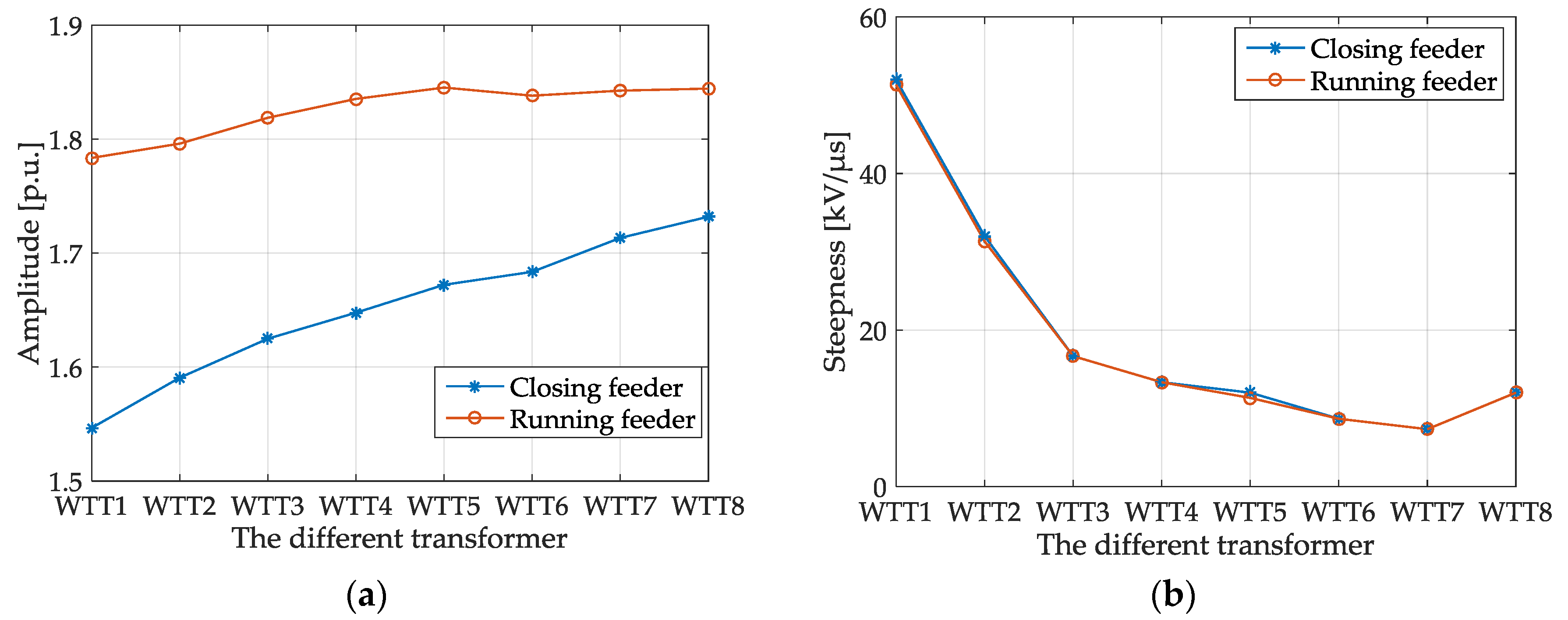
As shown in Figure 12, 2-1 means closing one feeder when two other feeders are running (Scenario 3, i.e., closing VCB1 when VCB2 and VCB3 have been closed). C refers to the feeder that is closed, and R refers to the feeders that are running. The overvoltage amplitude and steepness of Case 1-1 are chosen as the reference values. On the one hand, Figure 12 shows that, as the number of running feeders increases, the overvoltage amplitude and steepness of the closed feeder increase, while the overvoltage steepness increases by a factor of (2N/(N + 1)), where N is the number of running feeders. On the other hand, as the number of running feeders increases, the overvoltage amplitude and steepness of the running feeders decrease, and the overvoltage steepness decreases by a factor of (2/(N + 1)).
We also found that the overvoltage steepness of the closed feeders is N times larger than the steepness of the running feeders; additionally, we found that, regardless of the number of running feeders, the ratios of the overvoltage steepness of (WTT2–WTT8) transformers (which all have the same distance to the bus) to the overvoltage steepness of the WTT1 transformer (which is the closest to the bus when compared with the other transformers) are always constant. For example, the ratio of the overvoltage steepness of WTT2 to the overvoltage steepness of WTT1 is always equal to a constant y2; for WTT3 and WTT1, the ratio is always a constant y3. This relationship can be expressed by Equation (4):
where is the overvoltage steepness at the high voltage side of the transformer WTT1; is the overvoltage steepness at the high voltage side of the transformer WTTk; k = 2, 3, 4, 5, 6, 7, 8.
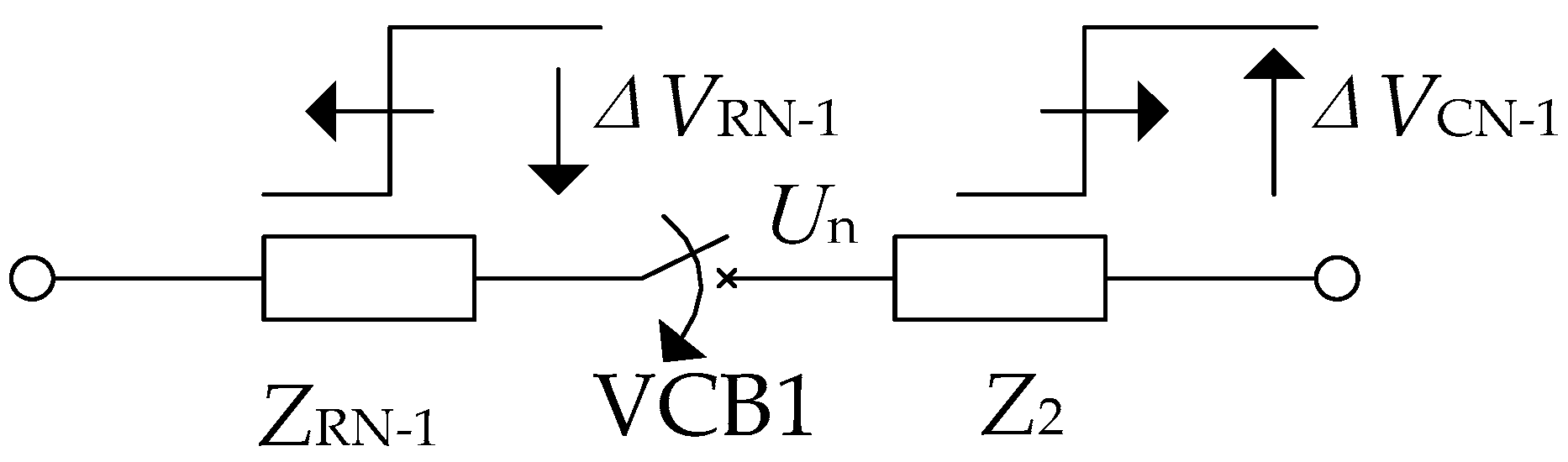
For Scenario 3, the voltage wave across VCB1 is shown in Figure 13. The ratio of transient voltage waves at both ends of VCB1 when VCB1 closes is calculated by Equations (5) and (6):
where is the incident voltage wave of the running feeders; is the wave impedance of the running feeders; is the incident voltage wave of the closed feeder; Z2 is the wave impedance of the closed feeder; and are the incident voltage waves of the closed feeder when the number of running feeders is one and N, respectively; is the voltage difference between both ends of VCB1.
Since the overvoltage steepness at the high voltage side of WTTs is proportional to the incident voltage wave of the feeders, the overvoltage steepness at the high voltage side of WTTs also satisfies the relationships in Equations (5) and (6). Thus, the simulation results are in good agreement with the theoretical analysis.
5. Conclusions
We have presented here HF modeling methodologies for VCBs, submarine cables, and WTTs. The prestrike model of the VCB looks at three parameters: the DS, the HF arc extinguishing capability, and the initial closing angle. For the cable modeling, the frequency-dependent (phase) model was adopted, and a hollow conductor layer was utilized. The transformer model takes into account the effect of stray capacitors on TOVs. A laboratory experimental platform for an OWF collection system was built and was used to verify the performance of the proposed models.
The developed models were used to analyze the effects of the initial closing angle of VCBs, along with different system operation scenarios on TOV amplitude and steepness. The results show that, when a feeder is closed when all the VCBs connected to it have also been closed and other feeders are still in service, as the number of running feeders increases, the overvoltage steepness of the closed feeder increases and the overvoltage steepness of the running feeders decreases. We also found that, when a WTT is closed and only one feeder is in service, the initial 15° phase angle will produce the largest overvoltage amplitude and steepness, along with the largest total number of prestrikes, and more attention should be paid to the impact of this condition on the turn-to-turn insulation of transformers in the design of electrical systems in OWFs.
This study shows that, in the future, it will be necessary to build an internal winding model for transformers to study the TOV distribution within the transformer winding. It would be helpful to study the impact of overvoltage steepness on winding insulation, along with measures that must be affected in order to suppress the impact.
Acknowledgments
This project was supported by the National Natural Science Foundation of China (No. 51477054). The authors would like to thank Xinyu Jiang from Guangzhou Zhiguang Electric Co. Ltd. for his support on experiments.
Author Contributions
This paper is a result of the collaboration of all co-authors. Gang Liu conceived and designed the study; Yaxun Guo established the model, implemented the simulations, and drafted the manuscript; Yanli Xin guided and revised the paper and refined the language; Lei You helped with most of the corrections; Xiaofeng Jiang helped establish the model and deal with the experimental data; Ming Zheng designed the experimental platform; Wenhu Tang built the experimental platform. All authors have read and approved the final manuscript.
Conflicts of Interest
The authors declare no conflict of interest.
Nomenclature
Variables
| Ub | dielectric strength between contacts of VCBs |
| TRVlimit | maximum DS that a VCB can withstand |
| A | rate of rise of DS |
| B | transient recovery voltage of VCB just before current zero crossing |
| t | time |
| tclose | the moment when a VCB begins to close |
| kaf | amplitude factor |
| kpp | first pole to clear factor |
| E_MAG | rated voltage of VCB |
| RS | parasitic resistance between contacts of VCBs |
| LS | parasitic inductance between contacts of VCBs |
| CS | parasitic capacitance between contacts of VCBs |
| IS | current flowing through VCBs |
| US | voltage at the entrance side of VCB |
| UL | voltage at the exit side of VCB |
| R0 | equivalent resistance of VCB |
| Vbrk | voltage difference across a VCB |
| u | voltage at the high voltage side of WTTs |
| i | current flowing through the phase-ground capacitor |
| CH | phase-ground capacitance |
| N | the number of running feeders |
| incident voltage wave of running feeders | |
| wave impedance of running feeders | |
| incident voltage wave of the closed feeder | |
| Z2 | wave impedance of the closed feeder |
| incident voltage waves of the closed feeder when the number of running feeders is one | |
| incident voltage waves of the closed feeder when the number of running feeders is N | |
| voltage difference between both ends of VCB1 |
Abbreviations
| VCB | vacuum circuit breaker |
| WTG | wind turbine generator |
| SOV | switching overvoltage |
| OWF | offshore wind farm |
| TOV | transient overvoltage |
| MV | medium voltage |
| HF | high frequency |
| WTT | wind turbine transformer |
| DS | dielectric strength |
| TRV | transient recovery voltage |
| UMEC | unified magnetic equivalent circuit |
| HV | high voltage |
| LV | low voltage |
References
- Liu, B.; Tang, W.H.; Chen, X.D.; Wu, Q.H. Modeling of transient overvoltages in wind power plants. In Proceedings of the 2014 IEEE Asia-Pacific Power and Energy Engineering Conference, Hong Kong, China, 7–10 December 2014. [Google Scholar]
- Mireanu, D. Transient Overvoltages in Cable Systems Part 1-Theoretical Analysis of Large Cable Systems. Master’s Thesis, Department of Electric Power Engineering, Chalmers University of Technology, Goteborg, Sweden, 2007. [Google Scholar]
- Boyra, M. Transient Overvoltages in Cable Systems Part 2-Experiments on Fast Transients in Cable Systems. Master’s Thesis, Department of Electric Power Engineering, Chalmers University of Technology, Goteborg, Sweden, 2007. [Google Scholar]
- King, R.; Moore, F.; Jenkins, N.; Haddad, A.; Griffiths, H.; Osborne, M. Switching transients in offshore wind farms-impact on the offshore and onshore networks. In Proceedings of the International Conference on Power Systems Transients, Delft, The Netherlands, 14–17 June 2011. [Google Scholar]
- Badrzadeh, B.; Hogdahl, M.; Isabegovic, E. Transients in wind power plants-Part I: Modeling methodology and validation. IEEE Trans. Ind. Appl. 2012, 48, 794–807. [Google Scholar] [CrossRef]
- Badrzadeh, B.; Zamastil, M.H.; Singh, N.K.; Breder, H.; Srivastava, K.; Reza, M. Transients in wind power plants-Part II: Case studies. IEEE Trans. Ind. Appl. 2012, 48, 1628–1638. [Google Scholar] [CrossRef]
- Liu, X.Z.; Wang, J.D.; Yishan, L.; Saboor, A.; Shang, Y.C.; Zhang, T.L. Simulating experiment and transient analysis on switching surges in cable collection grid of wind power plant. High Volt. Eng. 2014, 40, 61–66. [Google Scholar]
- Glasdam, J.; Bak, C.L.; Hjerrild, J. Transient studies in large offshore wind farms employing detailed circuit breaker representation. Energies 2012, 5, 2214–2231. [Google Scholar] [CrossRef]
- Liljestrand, L.; Sannino, A.; Breder, H.; Thorburn, S. Transients in collection grids of large offshore wind parks. Wind Eng. 2008, 11, 45–61. [Google Scholar] [CrossRef]
- Wang, J.D.; Li, G.J.; Qin, H. Simulation of switching over-voltages in the collector networks of offshore wind farm. Autom. Electr. Power Syst. 2010, 2, 104–107. [Google Scholar]
- Xin, Y.; Liu, B.; Tang, W.; Wu, Q.H. Modeling and mitigation for high frequency switching transients due to energization in offshore wind farms. Energies 2016, 9, 1044. [Google Scholar] [CrossRef]
- Villar, F.; Reza, M.; Srivastava, K.; Silva, L. High frequency transients propagation and the multiple reflections effect in collection grids for offshore wind parks. In Proceedings of the 2011 IEEE Power and Energy Society General Meeting, Detroit, MI, USA, 1–7 July 2011. [Google Scholar]
- Ghafourian, S.M.; Arana, I.; Holboll, J.; Sorensen, T.; Popov, M.; Terzija, V. General analysis of vacuum circuit breaker switching overvoltages in offshore wind farms. IEEE Trans. Power Deliv. 2016, 31, 2351–2359. [Google Scholar] [CrossRef]
- Gustavsen, B.; Martinez, J.; Durbak, D. Parameter determination for modeling system transients—Part II: Insulated cables. IEEE Trans. Power Deliv. 2005, 20, 2045–2050. [Google Scholar] [CrossRef]
- Wang, P.Y.; Liu, G.; Ma, H.; Liu, Y.G.; Xu, T. Investigation of the ampacity of a prefabricated straight-through joint of high voltage cable. Energies 2017, 10, 2050. [Google Scholar] [CrossRef]
- Abdulahovic, T.; Thiringer, T.; Reza, M.; Breder, H. Vacuum circuit breaker parameter calculation and modeling for power system transient studies. IEEE Trans. Power Deliv. 2017, 32, 1165–1172. [Google Scholar] [CrossRef]
- Rao, B.K.; Gajjar, G. Development and application of vacuum circuit breaker model in electromagnetic transient simulation. In Proceedings of the Power India Conference, New Delhi, India, 1–7 April 2006. [Google Scholar]
- Abdulahovic, T. Analysis of High-Frequency Electrical Transients in Offshore Wind Parks. Ph.D. Thesis, Department of Electrical Power Engineering, Chalmers University of Technology, Gothenburg, Sweden, 2011. [Google Scholar]
- Helmer, J.; Lindmayer, M. Mathematical modeling of the high frequency behavior of vacuum interrupters and comparison with measured transients in power systems. In Proceedings of the 17th International Symposium on Discharges and Electrical Insulation in Vacuum, Berkeley, CA, USA, 21–26 July 1996. [Google Scholar]
- Greenwood, A. Electrical Transients in Power Systems, 2nd ed.; Wiley: London, UK, 1991. [Google Scholar]
- Das, J. Surges transferred through transformers. In Proceedings of the Pulp and Paper Industry Technical Conference, Toronto, ON, Canada, 17–21 June 2002. [Google Scholar]
- Reza, M.; Breder, H. Cable System Transient Study: Vindforsk V-110: Experiments with Switching Transients and Their Mitigation in a Windpower Collection Grid Scale Model; Elforsk: Stockholm, Sweden, 2009. [Google Scholar]
- Dullni, E.; Sean-Feng, Z. Bouncing phenomena of vacuum circuit breakers. In Proceedings of the 24th International Symposium on Discharges and Electrical Insulation in Vacuum, Braunschweig, Germany, 30 August–3 September 2010. [Google Scholar]
- Zhang, T.; Sun, L.X.; Zhang, Y. Study on switching overvoltage in offshore wind farms. IEEE Trans. Appl. Supercond. 2014, 24, 1–5. [Google Scholar]
- Guo, Y.X.; Liu, G.; Jiang, X.F.; Liang, J.H.; Zheng, M. Simulation on overvoltage of internal electric system of offshore wind farm. Guangdong Electr. Power 2017, 10, 23–27. [Google Scholar]
Figure 1.
Simplified diagram of the investigated offshore wind farm (OWF).

Figure 2.
The cable arrangement.
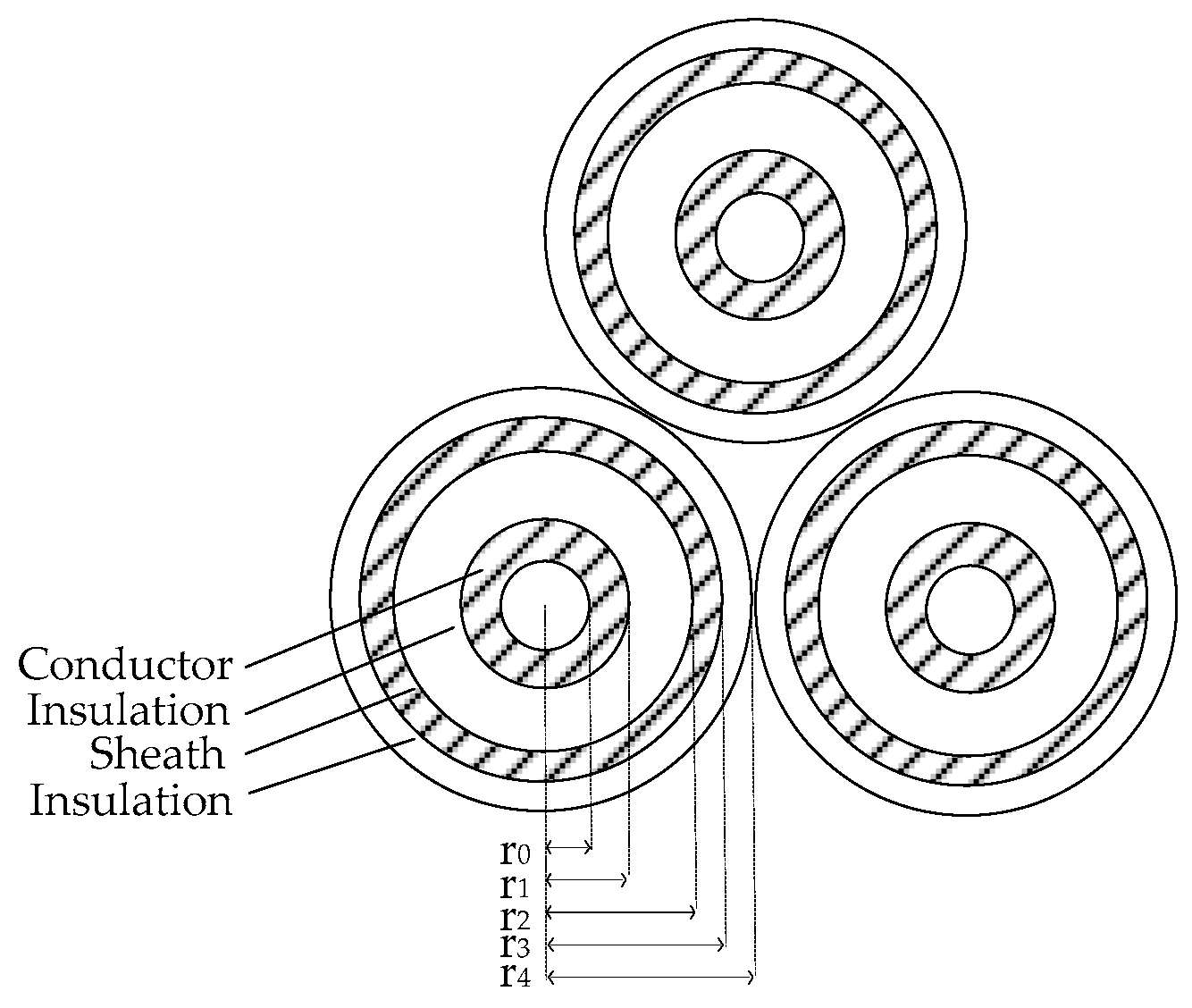
Figure 3.
The vacuum circuit breaker (VCB) model diagram.

Figure 4.
The program flow chart of the developed VCB model.

Figure 5.
The test system wiring diagram.
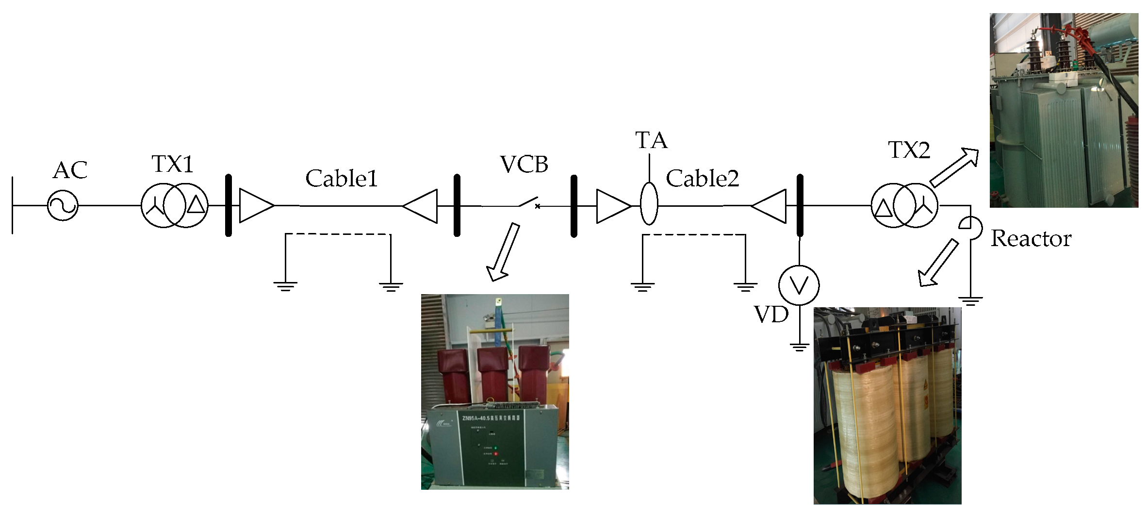
Figure 6.
Voltage and current waveforms at the high voltage side of TX2: (a) voltages; (b) currents.
Figure 6.
Voltage and current waveforms at the high voltage side of TX2: (a) voltages; (b) currents.

Figure 7.
The zoomed-in views of the voltages and currents at the high side of TX2: (a) voltages; (b) currents.
Figure 7.
The zoomed-in views of the voltages and currents at the high side of TX2: (a) voltages; (b) currents.
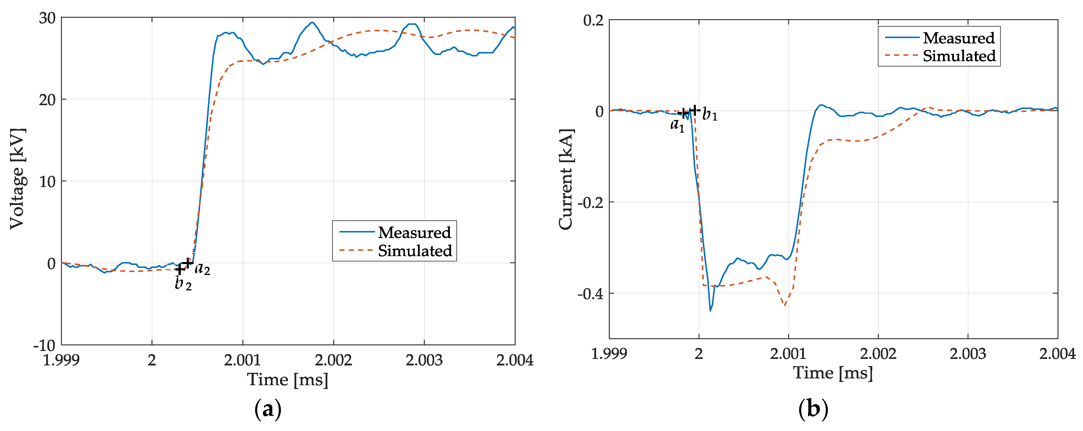
Figure 8.
The relationship between different indicators of TOV and the initial closing phase angle for Scenario 1: (a) the amplitude and steepness; (b) the number of prestrikes (#prestrikes).
Figure 8.
The relationship between different indicators of TOV and the initial closing phase angle for Scenario 1: (a) the amplitude and steepness; (b) the number of prestrikes (#prestrikes).
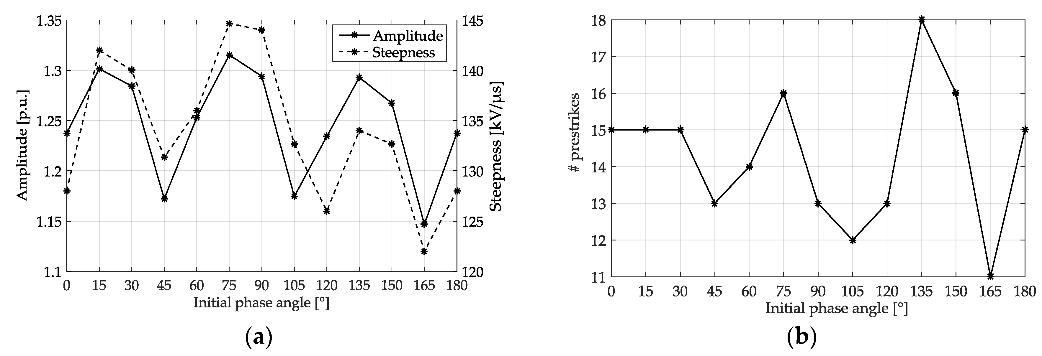
Figure 9.
The relationship between the initial closing angle and overvoltage.

Figure 10.
The overvoltage of different transformer locations for Scenario 2.

Figure 11.
The overvoltage of different transformer locations for Scenario 3: (a) amplitude; (b) steepness.
Figure 11.
The overvoltage of different transformer locations for Scenario 3: (a) amplitude; (b) steepness.

Figure 12.
The overvoltages for different transformers when the number of running feeders changes: (a) amplitude; (b) steepness.
Figure 12.
The overvoltages for different transformers when the number of running feeders changes: (a) amplitude; (b) steepness.
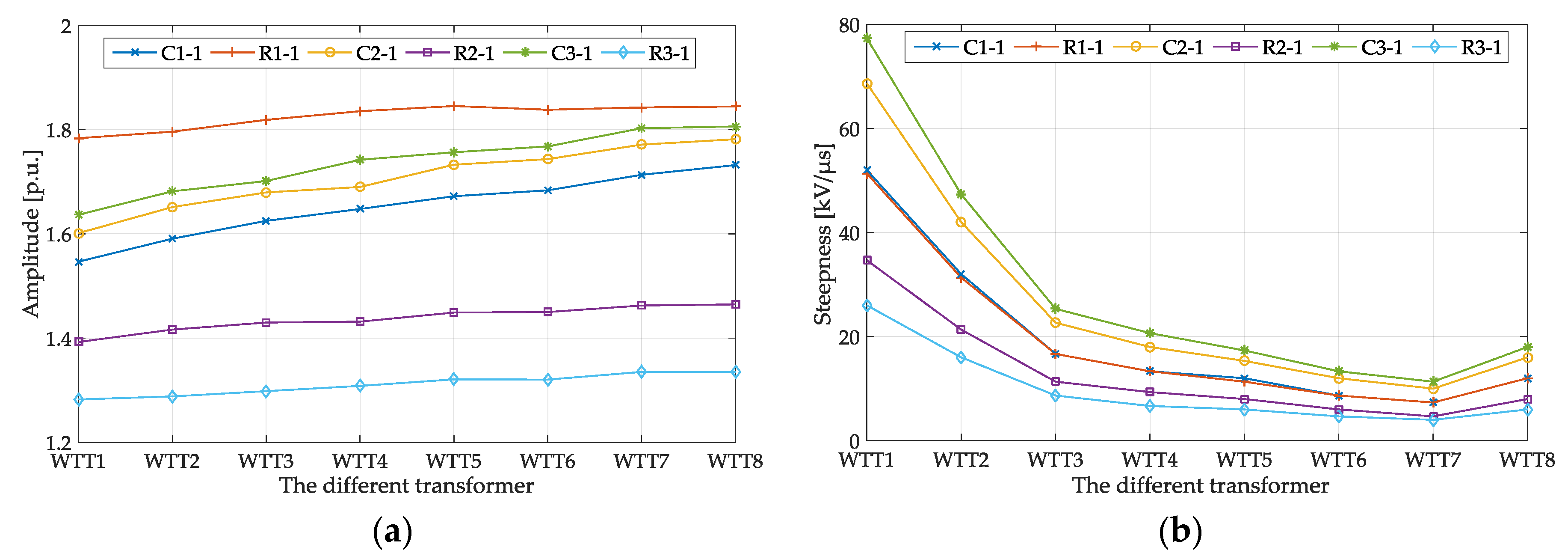
Figure 13.
The overvoltage waveform across VCB1.


Table 1.
The cable parameters and installation conditions.
| Structural Parameters | |||||
|---|---|---|---|---|---|
| r0 (mm) | r1 (mm) | r2 (mm) | r3 (mm) | r4 (mm) | |
| 3.255 | 10.3 | 20.8 | 22.9 | 24.9 | |
| Electrical Parameters | |||||
| Resistivity (Ω·m) | Relative Dielectric Constant | ||||
| Conductor | Metal Shield | Conductor Insulation | Shield Insulation | ||
| 1.92 × 10⁻⁸ | 2.2 × 10⁻⁷ | 2.5 | 2.3 | ||
| Installation Conditions | |||||
| Laying Depth (m) | Sea Water Resistivity (Ω·m) | ||||
| 1 | 1 | ||||
Table 2.
Typical stray capacitances of transformers.
| Transformer Capacity/MVA | HV-Ground Capacitance/nF | LV-Ground Capacitance/nF | HV-LV Capacitance/nF |
|---|---|---|---|
| 1 | 1.2–14 | 3.1–16 | 1.2–17 |
| 2 | 1.2–16 | 3–16 | 1–18 |
| 5 | 1.2–14 | 5.5–17 | 1.1–20 |
| 10 | 4–7 | 8v18 | 4–11 |
| 25 | 2.8–4.2 | 5.2–20 | 2.5–18 |
| 50 | 4–6.8 | 3–24 | 3.4–11 |
| 75 | 3.5–7 | 2.8–13 | 5.5–13 |
© 2018 by the authors. Licensee MDPI, Basel, Switzerland. This article is an open access article distributed under the terms and conditions of the Creative Commons Attribution (CC BY) license (http://creativecommons.org/licenses/by/4.0/).
Share and Cite
MDPI and ACS Style
Liu, G.; Guo, Y.; Xin, Y.; You, L.; Jiang, X.; Zheng, M.; Tang, W. Analysis of Switching Transients during Energization in Large Offshore Wind Farms. Energies 2018, 11, 470. https://doi.org/10.3390/en11020470
AMA Style
Liu G, Guo Y, Xin Y, You L, Jiang X, Zheng M, Tang W. Analysis of Switching Transients during Energization in Large Offshore Wind Farms. Energies. 2018; 11(2):470. https://doi.org/10.3390/en11020470
Chicago/Turabian StyleLiu, Gang, Yaxun Guo, Yanli Xin, Lei You, Xiaofeng Jiang, Ming Zheng, and Wenhu Tang. 2018. "Analysis of Switching Transients during Energization in Large Offshore Wind Farms" Energies 11, no. 2: 470. https://doi.org/10.3390/en11020470
Note that from the first issue of 2016, this journal uses article numbers instead of page numbers. See further details here.