An Improved Interval Fuzzy Modeling Method: Applications to the Estimation of Photovoltaic/Wind/Battery Power in Renewable Energy Systems


1
Research Center for Smart Vehicles and Electromagnetic Energy System Laboratory, Toyota Technological Institute, Nagoya 468-8511, Japan
2
Department of Electrical Engineering and Bioscience, Waseda University, Tokyo 169-8555, Japan
*
Author to whom correspondence should be addressed.
Energies 2018, 11(3), 482; https://doi.org/10.3390/en11030482
Submission received: 11 February 2018
/
Revised: 15 February 2018
/
Accepted: 17 February 2018
/
Published: 25 February 2018
(This article belongs to the Section F: Electrical Engineering)
Abstract
:This paper proposes an improved interval fuzzy modeling (imIFML) technique based on modified linear programming and actual boundary points of data. The imIFML technique comprises four design stages. The first stage is based on conventional interval fuzzy modeling (coIFML) with first-order model and linear programming. The second stage defines reference lower and upper bounds of data using MATLAB. The third stage initially adjusts scaling parameters in the modified linear programming. The last stage automatically fine-tunes parameters in the modified linear programming to realize the best possible model. Lower and upper bounds approximated by the imIFML technique are closely fitted to the reference lower and upper bounds, respectively. The proposed imIFML is thus significantly less conservative in cases of large variation in data, while robustness is inherited from the coIFML. Design flowcharts, equations, and sample MATLAB code are presented for reference in future experiments. Performance and efficacy of the introduced imIFML are evaluated to estimate solar photovoltaic, wind and battery power in a demonstrative renewable energy system under large data changes. The effectiveness of the proposed imIFML technique is also compared with the coIFML technique.
1. Introduction
In recent years, there has been rapid and significant development of renewable energy systems, including photovoltaic (PV) solar and wind power. Efficient control methods for managing renewable energy resources have also been designed and implemented. The high uncertainty of weather conditions makes forecasts of power profiles from renewable energy resources important for energy management, especially in large solar PV and wind power plants [1,2]. The time horizon of estimating and forecasting methods can be divided into very short-term, short-term, medium-term and long-term predictions [1]. The very short-term forecast is for a period of a few seconds to a few minutes. The short-term forecast is for a period of several minutes to three days. The medium-term forecast is for a period of several days to one week. The long-term forecast is for a period of one month to several years. The medium-term and long-term energy forecasts are usually computed on a large centralized server of energy producers or utility companies with big data. Depending on renewable power profiles and desired purposes in grid operations, the very short-term and short-term forecasts can be calculated on either decentralized systems such as modern personal computers or industrial programmable logic controllers (PLCs), or a centralized server of utility company. The resolution of estimating and forecasting energy models is classified according to the kinds of methods, measurement sensors and meteorological information in use. It often includes the temporal resolution [2], spatio-temporal resolution with the required forecast horizon and update frequency [2,3,4], measured dataset resolution [4,5,6], and satellite image resolution with image processing techniques [7]. The very short-term and short-term predictions of renewable power are closely related to high temporal resolution.
In renewable energy management systems (EMSs) and smart grid operations, the very short-term and short-term predictions of renewable power are especially helpful for lots of crucial activities and applications, such as operations of solar PV and wind power systems, real-time dispatching and coordinating of generation units, control of energy storage systems, making decisions of grid operation and stability, and electricity market [1,6]. In cases of the small or medium renewable power profile, the short-term prediction can be utilized for local management of private resources and ancillary services, such as frequency regulation and voltage stability at local electric grids. Whereas, in cases of the large renewable power profile, the short-term prediction can be used for supporting global management of distributed generation in smart grids and power limitations through demand/response capabilities. Hence, many studies have concentrated on designing and carrying out efficient modeling techniques for short-term prediction of renewable power [4,5,6,7,8]. In this paper, we mainly focus on the short-term day-ahead estimation for solar PV, wind and battery power using measured two-dimensional data with the horizontal axis of time.
According to Wan et al. [1], prediction methods for renewable energy can be divided into three main types as follows: the first type is based on actually measured data of renewable energy generation systems. The second type is developed from historical measured data of explanatory variables, such as related weather parameters, consisting of solar radiation, wind speed and direction, cloudiness, air temperature, humidity, and so forth. The third type is hybrid forecast methods with appropriate combination of machine learning algorithms and numerical weather prediction (NWP) techniques for specific applications. More details can be found in section II of reference [1] and section 2 of reference [6].
Optimization has been a useful tool and widely applied in modeling and control techniques for renewable energy systems [9,10,11]. As presented in [10], a delay estimator of perturbation produced by unknown delay was designed to implement in the pitch control for wind turbine power conversion systems. The compensation from the proposed estimator is used to eliminate influence from the perturbation of unknown delay to the output power of wind turbine. As a result, the measured output power of wind turbine highly corresponds to the ideal output value of the optimal model without effect from unknown delay. This is to enhance performance and efficacy of the introduced pitch control technique substantially. This method also considered variable wind speed for estimating the output power of wind turbine power conversion system, and it has good performance. Regarding application aspect of the research, this method has not yet been extended to be a universal method for estimating other two-dimensional renewable power profile (such as solar PV power) or battery bank power in renewable energy systems. Furthermore, in [11], a hybrid estimator was used for the proportional-integral-derivative controller of a wind turbine power conversion system with appropriate identification of stability ranges for key system parameters. This estimation method has suitably incorporated the particle swarm optimization technique and the algorithm based on radial basis function neural network. The designed estimator has good performance under a fixed wind speed of 15 m/s. Nonetheless, this research has not yet considered the case of variable wind speed, which leads to large fluctuation in wind power profile.
Besides, modeling methods based on artificial neural networks or genetic algorithms for predicting the renewable energy were proposed in [12,13,14,15]. Specifically, an efficient modeling method using an artificial neural network and statistical feature parameters of solar radiation and ambient temperature were introduced in [12]. The input vector is appropriately rebuilt using several statistical feature parameters for radiation and ambient temperature to reduce model complexity. Furthermore, ref. [13] developed two adaptive neuro-fuzzy models with several scenarios. The first scenario was designed by modifying the forecasting time horizon, and the second scenario adjusts shapes of the fuzzy membership functions. A generalized model for solar power prediction based on the backgrounds of support vector regression, historical solar energy output, and meteorological data was presented in [14]. Also developed was a model fine-tuned with a genetic algorithm and data mining algorithms for historical situations of predicted values for weather parameters [15]. Data for training this model were obtained using numerical methods for weather forecasts and previous electric energy values in the solar PV power plant. These methods have good effectiveness, but their computation is relatively complex and training processes can be long. In addition, these methods are often used for medium-term and long-term predictions instead of short-term prediction. To appropriately implement these methods in actual EMSs, high-performance computers should be used.
The traditional Takagi-Sugeno (T-S) fuzzy model [16,17,18,19,20] and belief rule-based models for identification [21] are popular modeling techniques for nonlinear systems. In [16], the T-S model was applied for process control. In [17], the modeling and control techniques based on T-S fuzzy models were introduced and explained in detail. In this study, the predictive controller based on T-S fuzzy model was also proposed. In [18], an application of input-output T-S fuzzy model for identification of multi-input and multi-output (MIMO) systems was presented and evaluated. In [19], modeling techniques based on fuzzy models, including T-S fuzzy models, were investigated. In [20], a robust fault estimation and fault-tolerant control approach was proposed for T-S fuzzy systems by integrating the augmented system method, unknown input fuzzy observer design, linear matrix inequality optimization, and signal compensation techniques. This approach was applied for wind turbine. However, the result of T-S fuzzy modeling is a trajectory, which is unsuitable for large variation in renewable power profile that highly depends on weather conditions. This is a common drawback of modeling methods based on T-S fuzzy model. Moreover, a hybrid two-stage modeling technique based on fuzzy logic, optimization, and model selection was proposed to predict day-ahead electricity prices as shown in [22]. In that technique, the first design stage is appropriate combination of the particle swarm optimization and core mapping with a self-organizing map and fuzzy logic, and the next design stage is appropriate selection of fuzzy rules. However, estimation of power profiles from PV and wind energy systems has not yet been considered in this research.
According to the reviews in [1,6,9], fuzzy logic can provide a robust and advantageous modeling method and can be suitably applied to short-term and medium-term forecasting models, since it can effectively handle uncertainty in measured data. A conventional interval fuzzy modeling (coIFML) technique based on -norm, min–max optimization methods, and linear programming was introduced in [23]. This model defines lower and upper bounds that cover all data points, and was widely applied to fault detection in various systems, including a process with interval-type parameters [24], uncertain nonlinear systems [25,26,27], an active suspension system [28], the pH titration curve [29], and power control of a Francis water turbine [30]. In addition, the coIFML technique was utilized to forecast PV and wind power and load profiles in microgrids [31], and it was implemented as a main component of prediction in robust EMSs [32,33]. One main advantage is a computed confidence band, which lies between the approximated lower and upper bounds of the coIFML, and can cover all measured values even under relatively large data variation. Furthermore, computation is not complex. Its robust band thus makes this method suitable for estimating renewable power profiles. Nonetheless, the coIFML confidence band is highly conservative and not well fitted to the data, especially cases in large variations and strong nonlinearities. A fitted estimator is important and necessary for an EMS to predict the total power capacity exactly and generate appropriate control commands for the power system. Moreover, performance and effectiveness of both the coIFML technique and T-S fuzzy model [16,17,18,19,20] heavily depend on fuzzy membership functions, which are often chosen manually and difficult to optimize.
The above observations and motivations suggest the need for an efficient estimation method based on interval fuzzy model that can overcome the following engineering challenges. First, the newly proposed method can fit data with large variation and strong nonlinearities to improve performance noticeably, as well as it can inherit good robustness and applicability of the coIFML in estimating solar PV and wind power profiles with short-term prediction. In addition, performance and efficacy of the suggested fuzzy-based method should not heavily depend on manual determination of fuzzy membership functions as the coIFML and T-S fuzzy model techniques. Furthermore, to facilitate application in actual renewable EMSs, computation in the proposed modeling method should not be too complex. Last, this estimation method would possibly help enhance development and implementation of robust EMS (REMS) in renewable power systems.
This paper introduces an improved interval fuzzy modeling (imIFML) technique that is based on first-order models, modified linear programming, and actual boundary data points. The main contributions of this paper are as follows:
- (a)
- The four design stages of the proposed imIFML technique are described in detail. The third and fourth stages, which suitably adjust the approximated lower and upper bounds of the imIFML technique to fit the reference bounds closely, are newly developed. The modified linear programming scheme in the imIFML technique is unique and has good efficacy.
- (b)
- The performance of the proposed imIFML is significantly less conservative than the coIFML, especially in cases of large variation in data. Robustness and applicability are inherited from the coIFML. In addition, computation in the imIFML technique is not exceedingly complex.
- (c)
- The proposed imIFML technique is suitable for estimating solar PV, wind and battery power in a demonstrative renewable energy system over 24 h under large variation and strong nonlinearities in the measured data, which was used for a REMS. The specific test cases considered in this study are for users in private EMSs. Because the proposed imIFML technique is based on a modified linear programming scheme, computation in this modeling technique is not very complicated. Therefore, the proposed imIFML can be performed well with a pretty modern personal computer. In our study, all the three test cases are easily conducted with a desktop computer, and the processing time is within a few minutes.
- (d)
- Sample MATLAB Optimization Toolbox code for developing fuzzy models is provided for reference in future experiments and related applications.
To fulfill the above goals, a unique modified linear programming scheme is developed for the imIFML method. In the scheme, two scaling matrices and are newly added for suitably adjusting two coefficient matrices and of the modified linear programming, respectively. This helps to regulate arbitrary values and around the actual boundary points and of data to be equal to the minimum values of nearly zero, respectively. As will be presented in the Section 3.4, the two scaling matrices and are automatically fine-tuned to achieve the best possible fuzzy model. Moreover, due to the changeable coefficient matrices and in the modified linear programming, effectiveness and adaptability of the imIFML technique are not heavily dependent on manual determination of particular values for fuzzy clusters (membership functions). In this study, although the membership functions are determined by using a simple averaging method, performance and adaptability of the proposed imIFML are still very good.
The remainder of this study is organized as follows: Section 2 describes the core background of the coIFML. Section 3 presents the four design stages of the proposed imIFML technique. Section 4 presents simulation results for three test cases in Optimization Toolbox, including cases that consider the effects of large variation in the measured data. This section also compares the efficacy of the proposed imIFML technique and the coIFML. Section 5 presents additional helpful discussions for future experiments using the proposed imIFML technique. Finally, Section 6 concludes this paper and describes future work.
2. Backgrounds of Interval Fuzzy Model
This section briefly presents core background on the interval fuzzy model, which is known as a robust system identification technique. Further details of the model can be found in [23,26].
It is given that D ⊂ R is a data set and ξ = {ν(w): D → R} is a class of nonlinear functions. It is assumed that there may exist a lower bound ν and an upper bound that can fulfill the following conditions for the arbitrary values and for each input variable:
This study is only restricted to the finite set of the measured input data W = [w1, w2, …, wN] and the finite set of the measured output data Y = [y1, y2, …, yN] where N is the size of the input and output data sets. The conditions in Equations (1) and (2) can be rewritten as Equations (3) and (4):
The exact lower and upper boundary functions ν and will be approximated by fuzzy functions. According to [23,26], there may exist two fuzzy systems, denoted as and , that respectively approximate the lower and upper bounds to cover an arbitrary nonlinear acreage. The key goal of fuzzy approximation is to force the two non-negative values and in Equations (1) and (2) to be small as possible:
In this study, the first-order model is chosen to be used for the coIFML based on Takegi-Sugeno type as defined in the affine form by Equation (7). Values of the scalar coefficients , , and need to be appropriately determined to achieve an excellent fuzzy model as possible:
where the antecedent variable xad = inputf ∈ R represents the input variable in fuzzy proposition, and the approximated variables , are the two outputs of the interval fuzzy model [26]. The confidence-band identification of the fuzzy model is the interval between the bounds and .
The antecedent variable is associated with k fuzzy sets denoted as . Each the fuzzy set (j = 1, …, k) is linked to a real-valued function expressed as , which generates a particular membership level of the antecedent variable with correlation to the computed fuzzy set . It is noted that k is the number of fuzzy rules, and must be not larger than the data size, k N. The consequent vector in the affine form is denoted as . The first-order fuzzy model expressed in Equation (7) can be rewritten in the general form as follows:
where and are the lower and upper coefficient matrices for the full set of the fuzzy rules, respectively; is a vector of standardized membership functions with components which signify the grade values of accomplishment to the corresponding fuzzy rules, where can be computed as follows:
As represented in [23,24,25,26], the min-max optimization technique and -norm can be utilized for developing the interval fuzzy model as expressed in Equation (10). This equation is often realized into the linear programming approach to determine the coefficient matrices and for the approximated lower bound and upper bound of the coIFML, respectively. The detailed realization and implementation of the linear programming for the coIFML will be shown in Section 3.1.
3. Design Stages of Proposed Improved Interval Fuzzy Modeling
The proposed imIFML technique—which uses the first-order model in Equation (7), modified linear programming, and actual boundary data points to overcome the drawbacks of the coIFML scheme—consists of four design stages. The first stage (Section 3.1) is describing the detailed implementation process of the coIFML using a first-order model and linear programming in MATLAB Optimization Toolbox (version 7.1, The MathWorks, Inc., Natick, MA, USA) for reference and evaluation. In the second stage (Section 3.2), we use MATLAB to define the lower and upper reference bounds for designing the proposed imIFML technique according to comparison between the approximated bounds of the coIFML and the actual data boundaries. In the third stage (Section 3.3), the major drawbacks of the coIFML are described according to the performance and analysis shown in the first two stages. After that, key points of the modified linear programming used in the introduced imIFML technique are presented. This design stage is also the initial adjustment for the scaling matrices of the modified linear programming in the proposed imIFML technique. In the final stage (Section 3.4), the scaling matrices of the modified linear programming in the imIFML technique are automatically fine-tuned to obtain the best fuzzy model possible.
Panels (a) and (b) of Figure 1 depict the first and second design stages, respectively. This paper denotes two-dimensional finite data as (x, y) and the data size as N. Note that x is the time (horizontal axis) and that y (vertical axis) is converted to per-unit (pu) values for convenience when developing and tuning the fuzzy models.
3.1. Design Stage 1: The coIFML with First-Order Model and Linear Programming
As depicted in panel (a) of Figure 1, this design stage is to describe implementation steps of coIFML using MATLAB Optimization Toolbox linear programming. This provides a useful background for reference when applying the coIFML in related applications.
Clustering methods such as Gustafon–Kessel, K-means, or C-means can be used to determine particular fuzzy cluster values [34,35]. To evaluate performance and efficacy of the proposed imIFML technique with the modified linear programming, we apply simple clustering based on the averaging method to determine the particular values of fuzzy clusters as expressed in Equations (11) and (12):
where is the number of fuzzy clusters (membership functions) for the model, and 2 N; dis is the distance value between the two consecutive fuzzy clusters:
In this study, the two-dimensional data (x, y) used to develop the fuzzy model is assumed within a period of 24 h, where min(x) = 0 h, max(x) = 24 h, and the applications are realized for the PV/wind/battery power system within one day. The number of the fuzzy clusters is chosen as = 24. From Equations (11) and (12), the particular values of the fuzzy clusters are shown in Figure 2.
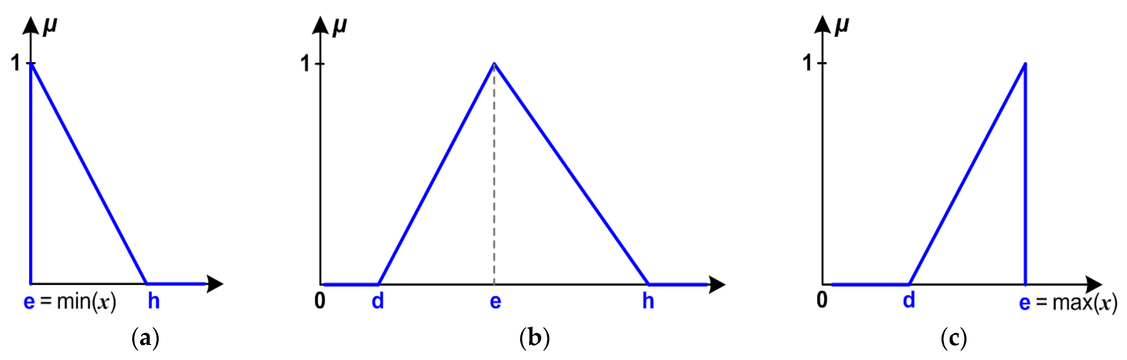
To implement the linear programming of the coIFML in MATLAB, the mathematical functions for the three kinds of triangle membership functions in Figure 2 should be realized as depicted in Figure 3 and Equations (13)–(15). The mathematical equations for representing the membership functions in panels (a), (b), and (c) of Figure 3 are expressed in Equations (13), (14), and (15), respectively.
With the antecedent vector , from Equations (9) and (13)–(15), the vector of standardized membership functions is as:
It is noted that N is the size of the data for developing the fuzzy model, and k is the number of fuzzy clusters (membership functions), where its value is chosen as k = 24 in this study.
• Detailed implementation of linear programming for the lower bound of the coIFML
With the first-order model shown in Equation (7), the value array of the coefficient matrix for the lower bound of the coIFML is expressed in Equation (17):
where the fuzzy antecedent vector is , and the consequent vector is represented in the affine form as , the lower bound at the first equation in Equation (8) is realized as follows:
For convenience in programming, where y is the data set in vertical axis, Equation (5) now can be rewritten as:
From Equations (18) and (19), the relevant matrices , and used to approximate the lower bound by linear programming in MATLAB/Optimization are presented in Equation (20):
where
and:
• Detailed implementation of linear programming for the upper bound of the coIFML
With the first-order model shown in Equation (7), the value array of the coefficient matrix for the upper bound is shown in Equation (21):
where the fuzzy antecedent vector is , and the consequent vector is represented in the affine form as , the approximated upper bound at the second equation in Equation (8) is realized as follows:
For convenience in programming, where y is the data set in vertical axis, Equation (6) now can be rewritten as:
From Equations (22) and (23), the relevant matrices , and used to approximate the upper bound by the linear programming in MATLAB/Optimization are shown in Equation (24):
where
and:
In this study, the linear programming can be executed using the command linprog in the Optimization toolbox of MATLAB [36]. The sample code in MATLAB to implement the coIFML (also the first stage of the imIFML) with parameters in Equations (20) and (24) is presented in Appendix A.
3.2. Design Stage 2: Determine the Actual Boudnaries of Data, and Reference Lower and Upper Bounds
In this stage, actual boundary points of the two-dimensional data (x, y) used for modeling are determined as described in Figure 1 panel (b). After that, two reference bounds for adjusting the approximated lower and upper bounds of the proposed imIFML technique are determined.
An efficient concave boundary algorithm for datasets can be found in [37]. We use the MATLAB boundary command [38] to determine the boundary points of two-dimensional data. The syntax of this command is boundary(x, y, θ), where x is the horizontal axis data, y is the vertical axis data, and θ is the shrink coefficient with a scalar value in the range of [0, 1]. If θ is set to 0 this gives a convex hull, and if θ is set to 1 this gives a tight boundary that covers the data points. The default value of the shrink coefficient θ is 0.5.
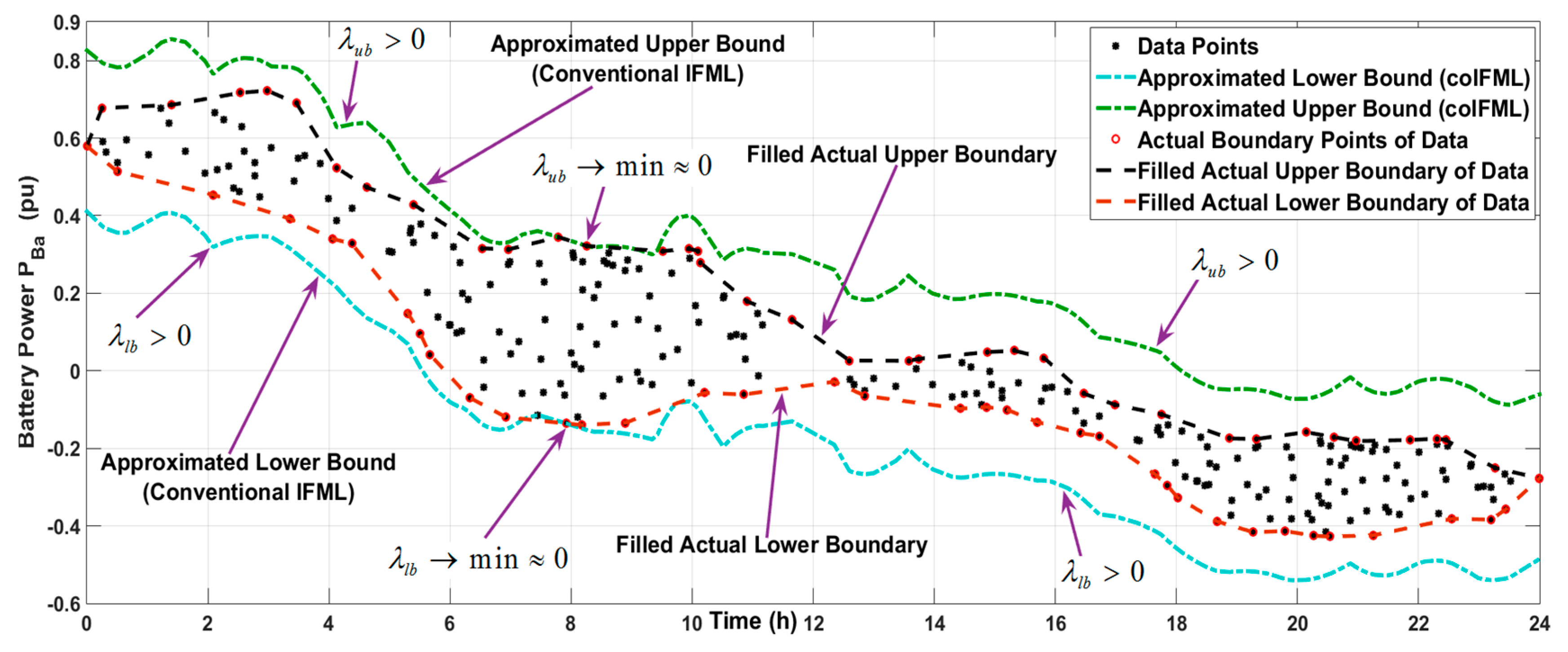
For example, the return value of the boundary command with θ = 0.73 for battery power data is an index vector of boundary points, as depicted in Figure 4. The index vectors of actual lower and upper boundary points are denoted as = [,…,,…,] and = [,…,,…,], respectively, where = 1 and = N. In this example, = 37, = 38, and N = 280. The value vectors of the actual lower and upper boundary points on the vertical axis are given as and , respectively. Figure 5 shows the actual boundary data points, which are marked with red circles.
As depicted in Figure 4, the sizes of and are smaller than the size of the data, meaning that < N and < N. To suitably design the proposed imIFML technique, the number of points in the actual lower and upper boundary vectors should use N as the data size. The procedures for conducting this task are described in the third execution block (from the top) in Figure 1 panel (b). Specifically, the linear function for two consecutive points in the actual lower- or upper-boundary vector is easily determined. After that, linear functions for all consecutive points in the lower- and upper-boundary vectors are established, responses to which are respectively illustrated by the red and black dashed lines in Figure 5. Finally, virtual data points on the vertical axis, which reflect the horizontal-axis dataset x to the defined linear functions, will additionally be filled in the actual lower- and upper-boundary vectors and . As a result, the sizes of the newly filled actual boundary vectors and now are N, the same size as dataset y.
With the filled actual boundary vectors and , the reference bounds and for adjusting the approximated lower and upper bounds of the proposed imIFML technique are defined as:
The two ratio matrices and between the approximated lower and upper bounds of coIFML and their reference bounds in Equation (25) are determined as:
3.3. Design Stage 3: Initially Adjust the Scaling Parameters in the Modified Linear Programming
As shown in Equations (20) and (24), all linear programming matrices used in the coIFML have fixed values. Hence, the linear programming response when approximating the lower and upper bounds in Equations (19) and (23) can only regulate arbitrary values and to the minimum values at several regions in the data. This means that and may exceed the minimum values in other data regions. Especially in cases of data with large variation, the difference between the defined minimum values and the arbitrary values in other regions may be very large. For example, as shown in Figure 5, and approach their minimum values of nearly zero around the region of t = 8 h. Meanwhile, in the regions where t = [0 h, 5 h] and t = [11 h, 24 h], and are much larger than zero because the lower and upper bounds of the coIFML are far from the actual lower and upper boundaries. To overcome this issue, additional scaling matrices should be used to adjust the coefficient matrices and , which regulate and in the regions around the actual boundary points to be equal to the minimum values of nearly zero.
The modified linear programming used for the proposed imIFML technique is given in Equations (28) and (29), where the symbol ⊙ denotes element-wise multiplication. Here, values for matrices , , and are fixed to those of the coIFML given in Equations (20) and (24). Meanwhile, matrices and can now be suitably adjusted using newly-added scaling matrices and . Specifically, key points of the scaling matrix are that its element values can be different and changeable. The particular value of each matrix element is related to the same-order element in the ratio matrix in Equation (26), and the relation between them is shown in Equation (33). As a result, where the coefficient matrix is now online changeable, in Equation (19) will be considered an arbitrary matrix with element values regulated to be almost equal to the minimum value of nearly zero at the actual-data lower boundary points. This means that the computed lower bound of the proposed imIFML technique is appropriately driven to closely fit to the reference lower bound given by Equation (25) in most regions, especially at the actual lower boundary points. Similar conduct and explanation can be applied to the scaling matrix of the coefficient matrix for the upper bound in Equation (29), where the relation between and is expressed in Equation (35). To guarantee a proper adjusting process, the check errors in Equations (36) and (37) between the computed bounds of the imIFML technique and the reference bounds must satisfy the conditions ≥ 0 and ≥ 0, as will be described in the next subsection:
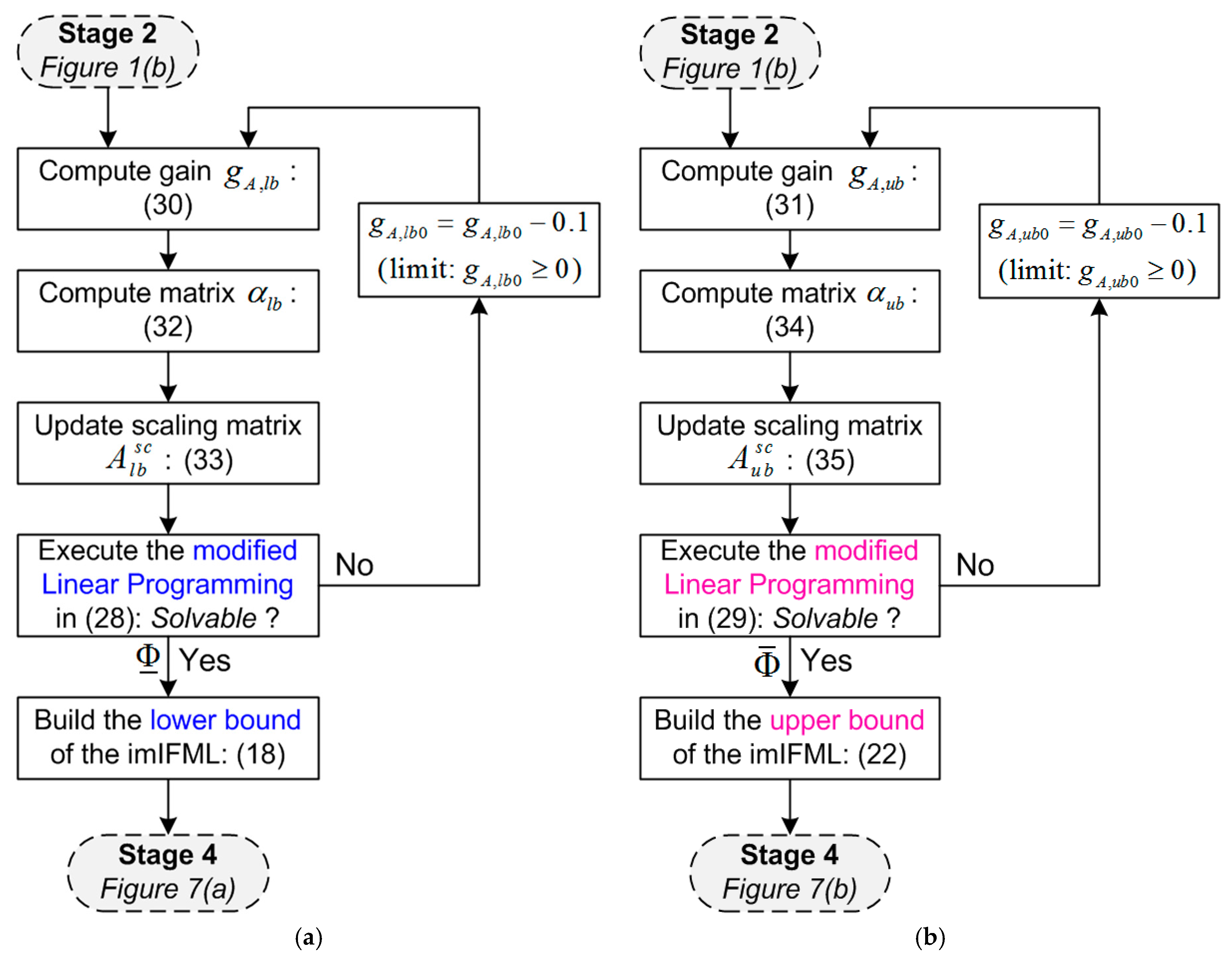
This design stage is the initial adjustment for the two scaling matrices and in the modified linear programming scheme given by Equations (28) and (29), respectively. The adjustment is performed simultaneously. The goal is to force the approximated lower and upper bounds of the proposed imIFML to move toward the reference bounds. Figure 6 panels (a) and (b) show detailed process diagrams of this stage for the lower and upper bounds of the proposed imIFML.
With the scale indexes determined using the MATLAB boundary command, the scalar scaling gains and are computed by Equations (30) and (31), respectively, where initial values and should be chosen in the interval of [0, 1]. In this study, and are chosen as 0.8, which is equivalent to 80% of 1 pu. This means that the reserve value of 20% can be used for fine-tuning, as will be shown in the next design stage. If the modified linear programming problems are not resolvable, the initial gain values and are reduced to and , as seen in Figure 6 panels (a) and (b), respectively.
here, r and are indexes on the actual boundary vectors and in Figure 4, and are the two reference bounds defined in Equation (25) at the second stage, and and are the bounds of the coIFML shown in Equations (18) and (22) at the first stage.
• For the approximated lower bound depicted in Figure 6 panel (a):
where is in Equation (30) and sgn() is the sign function, the intermediate matrix is computed as:
where the matrix is defined in Equation (26), and the scaling matrix for the lower bound in Equation (28) is calculated as:
• For the approximated upper bound illustrated in Figure 6 panel (b):
In this case, the intermediate matrix in Figure 6 panel (b) is computed as:
where is shown in Equation (31).
The scaling matrix for the matrix of the upper bound in Equation (29) is calculated as:
where is expressed in Equation (27).
Appendix B presents sample code for implementing the third design stage of the proposed imIFML in MATLAB Optimization Toolbox [36].
3.4. Design Stage 4: Automatically Fine-Tune the Parameters in the Modified Linear Programming
In this stage, the two scaling matrices and of the modified linear programming in Equations (28) and (29) are fine-tuned automatically. The tuning process is conducted in loops until a good model emerges. The objective is online adjustment for the approximated lower bound and upper bound of the proposed imIFML technique to be fitted to the reference bounds and in Equation (25) as closely as possible. Figure 7 panels (a) and (b) show detailed process diagrams of this design stage for the approximated lower and upper bounds.
From the two constraints in Equation (10), the scalar check errors at the actual boundary data points depicted in Figure 4 and Figure 5 are defined by Equations (36) and (37) for the tuning process in Figure 7 as:
where r and are the indexes of the actual boundary vectors and in Figure 4, respectively; 1 and 1 are the iteration indexes of loops in Figure 7 panels (a) and (b), respectively.
• For the approximated lower bound described in Figure 7 panel (a)
In this design stage, a new intermediate scalar gain is defined as below:
where the initial base value is chosen as 0.05, as equivalent to be 5% of 1 pu.
The intermediate matrix shown in Figure 7 panel (a) is updated online as follows:
where , and is computed in Equation (32). The ratio matrix is defined as:
where , and the matrix is calculated in Equation (26) at the second design stage.
The scaling matrix used for the matrix in Equation (28) now is online fine-tuned as below:
where is online updated in Equation (39), and it is noted that is computed in Equation (26) at the second stage. For the next iteration step of the tuning process, the iteration index is updated as follows:
where the initial value of the iteration index is . The limit of is set as to avoid the unexpected case of an infinite loop. In this study, the limit value is chosen as 500.
As shown in Figure 7 panel (a), if < 0 and = 0, this means that the initial value of the gain = 0.8 in Equation (30) is not chosen appropriately. Hence, the gain needs to be reduced as , and the tuning process returns to the third design stage in Figure 6 panel (a).
• For the approximated upper bound presented in Figure 7 panel (b)
In this design stage, a new intermediate scalar gain is defined as:
where the initial base value is chosen as 0.05, as equivalent to be 5% of 1 pu.
The intermediate matrix in Figure 7 panel (b) is online updated as follows:
where , and is computed in (34). The ratio matrix is defined as
The scaling matrix utilized for the matrix in Equation (29) is automatically adjusted as below:
where is online updated in Equation (44), and it is noted that is computed in Equation (27) at the second design stage. The iteration index for the upper bound is updated as follows:
where the initial value of iteration index is . The limit of is set as to avoid the unexpected case of an infinite loop. In this study, the limit value is chosen as 500.
3.5. Additional Limits for Application Cases in Estimating Solar PV and Wind Power
Because the power obtained from the solar PV arrays or wind turbine is often non-negative value, the following additional limits should be used for the two approximated bounds of the proposed imIFML in cases of estimating solar PV and wind power as expressed in Equation (48):
4. Simulation Results
Figure 8 shows a REMS implementing the proposed imIFML technique as a demonstrative renewable energy system. Power is obtained from PV arrays and wind turbines to supply loads and deliver to the grid. The battery bank absorbs power when in charge mode and supplies power in discharge mode. We investigated and evaluated estimation of power from battery bank , PV arrays , and wind turbine . The base power for converting to pu values in the demonstrative energy system was chosen as 100 kW. In this research, all power data for developing the interval fuzzy models are expressed in pu values.
We present three simulation cases performed using MATLAB R2014b and its Optimization Toolbox solvers [36,38]. The first test case considers battery power estimation in the proposed imIFML technique with two battery-bank operational modes (Section 4.1). The second test case considers output power estimation for PV arrays under large changes in solar radiation (Section 4.2). The last test case considers estimation of wind turbine output power under large variation in wind speed (Section 4.3). Figure 2 shows particular values for fuzzy clusters in all three test cases. The initial gains and expressed in Equations (30) and (31) are chosen as 0.8, and limiting values and for the iteration process in Figure 7 are chosen as 500. Figure 9, Figure 10 and Figure 11 show results of the first, second, and last described cases, respectively. These figures also show the approximated lower bound (blue line) and upper bound (pink line) of the proposed imIFML technique and the imIFML confidence band (yellow). In addition, the coIFML scheme is implemented for all test cases for reference with the proposed imIFML technique.
4.1. Test Case 1: Estimating the Power of a Battery Bank
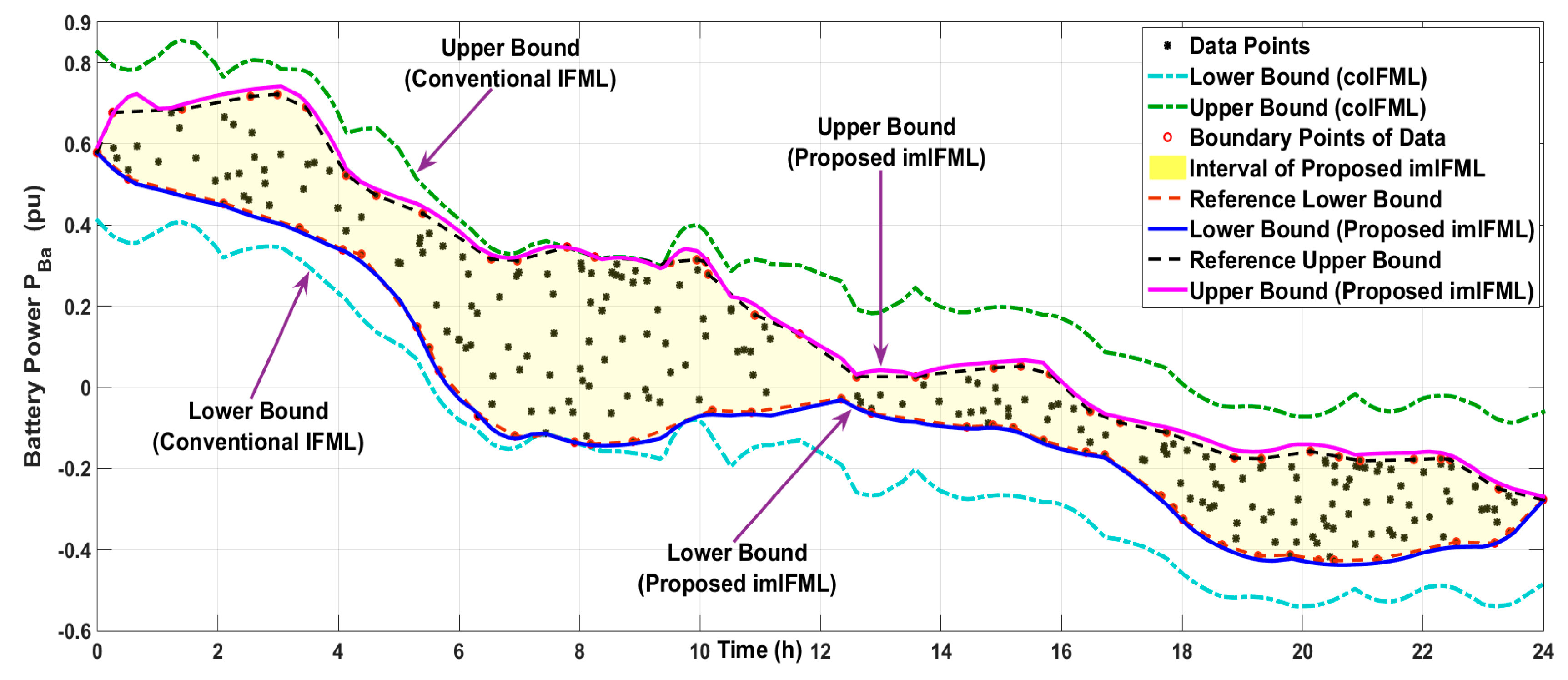
Figure 9 shows assumed operational data for the battery bank power. Namely, 0 pu indicates that the battery is in discharge mode, and 0 pu indicates that the battery is in charge mode. In this test case, the MATLAB boundary command, described in the second design stage (Section 3.2), was called as boundary(x, y, 0.73).
In panels (a) and (b) of Figure 7, the iteration values for tuning the lower bound and upper bound of the proposed imIFML technique were = 8 and = 9, respectively. The check errors in Equations (36) and (37) to stop the loops were = 0 and = 0, respectively.
Figure 9 shows performance in this test case. Under the coIFML method, the lower and upper bounds are highly conservative, especially for times t = 0 to 5 h and t = 11 to 24 h, and do not fit the lower and upper reference bounds. However, using the proposed scheme described in Figure 6 and Figure 7, the scaling matrices and of the modified linear programming in Equations (28) and (29) are automatically tuned and are highly consistent with variation in the data of battery power . This remarkably improves the response of the modified linear programming in the imIFML technique. As a result, the approximated lower and upper bounds under the proposed imIFML cover all the actual boundary data points, marked as red circles. The yellow band between the approximated lower and upper bounds covers all data points. For example, from time t = 0 to 2 h, the lower and upper bounds under the imIFML technique are suitably regulated to the reference data bounds, but the two coIFML bounds are not. The responses from time t = 14 to 16 h are similar. The check conditions for minimum error values at the boundary points in Equations (36) and (37) are also satisfied. This clearly demonstrates the salient efficacy of the proposed imIFML technique.
In real renewable power systems with stationary battery banks, the operation of systems often depends on forecasts of total power capacity, including battery power, and load demand. In this study, the main purpose of this test case is to evaluate performance and efficacy of the proposed modeling technique under large variation in battery power data. Estimation of battery power is helpful to predict maximum total power of the systems for efficiently controlling ancillary services, such as grid frequency regulation and voltage stability. Furthermore, the power obtained from battery banks is in both positive and negative values, which is useful to evaluate efficacy and adaptability of the proposed imIFML technique. On the other hand, the power obtained from PV arrays and wind turbines as well as load demand are often in positive values. Of course, the evaluation on efficacy of the proposed method in load demand forecast is also important, and it will be extensively studied in our future work.
4.2. Test Case 2: Estimating the Output Power of Solar PV Arrays
In this test, the weather condition is assumed in summer and with a clear sky at noon as depicted in Figure 10 to estimate the power obtained from solar PV arrays . In this case, the additional limits expressed in (48) are now applied for the approximated lower and upper bounds of the proposed imIFML. In this test case, the MATLAB boundary command, described in the second design stage (Section 3.2), was called as boundary(x, y, 1).
In panels (a) and (b) of Figure 7, the iteration values for tuning the lower bound and upper bound of the proposed imIFML technique were = 54 and = 62, respectively. The check errors in (36) and (37) to stop the loops were = 0 and = 0, respectively.
Figure 10 shows performance in this test case. Under the coIFML method, the lower and upper bounds are highly conservative, especially for times t = 4 to 9 h and t = 14 to 20 h, and do not fit the lower and upper reference bounds. However, using the proposed scheme described in Figure 6 and Figure 7, the scaling matrices and of the modified linear programming in Equations (28) and (29) are automatically adjusted and correspond to variation in the data of solar PV power . This substantially enhances effectiveness of the modified linear programming in the introduced imIFML. As a result, the computed lower and upper bounds under the imIFML technique cover all the actual boundary data points, marked as red circles. For example, from time t = 6 to 8 h, the lower and upper bounds under the imIFML technique are suitably regulated to the reference data bounds, but the two coIFML bounds are not. The responses from time t = 16 to 18 h are similar. The check conditions for minimum error values at the boundary points in Equations (36) and (37) are also satisfied.
Since the power obtained from the PV arrays is often a non-negative value, in this case, the lower bound of the proposed imIFML is applied with the additional limit given by the first equation in Equation (48). The responses of this additional limit are shown from the time t = 0 to 4.1 h and t = 20.1 to 24 h. The yellow confidence band between the computed lower and upper bounds covers all data points. This obviously shows the good performance and adaptability of the proposed imIFML technique.
4.3. Test Case 3: Estimating the Output Power of Wind Turbine
This test case considers estimation of the power obtained from the wind turbine under very large variation in the measured data as illustrated by Figure 11. The additional limits in (48) will be applied for the approximated lower and upper bounds of the proposed imIFML if the related conditions are satisfied. In this test case, the MATLAB boundary command, described in the second design stage (Section 3.2), was called as boundary(x, y, 0.97).
The iteration values for tuning the lower bound and upper bound of the imIFML technique in Figure 7 panels (a) and (b) are = 466 and = 467, respectively. In this test case, owing to the high variation in measured wind power, the iteration values and are significantly larger than in the two previous tests. The check errors at the actual boundary points in Equations (36) and (37) to stop the loops are still satisfied with = 0 and = 0.
Figure 11 shows performance in this test case. Under the coIFML method, the lower and upper bounds are highly conservative, especially for times t = 0 to 3 h, t = 9 to 11 h and t = 13 to 16 h, and do not fit the lower and upper reference bounds. However, using the proposed scheme described in Figure 6 and Figure 7, the scaling matrices and of the modified linear programming in Equations (28) and (29) are automatically altered, and are suitable with fluctuation in the data of wind power . This noticeably ameliorates performance of the modified linear programming in the imIFML method. As a result, the estimated lower and upper bounds under the suggested imIFML cover all the actual boundary data points, marked as red circles. For example, from time t = 5 to 7 h, the lower and upper bounds under the imIFML technique are suitably regulated to the reference data bounds, but the two coIFML bounds are not. The responses from time t = 14 to 16 h are almost same. The check conditions for minimum error values at the boundary points in Equations (36) and (37) are also satisfied.
Although the variation in data of wind power is large, the yellow confidence band between the two estimated lower and upper bounds of the proposed imIFML still covers data points pretty well, especially at the actual boundary points of data, because the two error values in Equations (36) and (37) are checked at these actual boundary points. This confirms the good adaptability of the suggested imIFML technique under high variation and nonlinearity in the data.
5. Additional Discussions
In some unexpected cases, the value of the computed lower bound under the proposed imIFML is slightly smaller than the one under the coIFML, and the value of the computed upper bound under the proposed imIFML is slightly larger than the one under the coIFML. Therefore, to enhance the robustness and efficacy of the final fuzzy model, the additional selections in Equation (49) can be applied for the proposed imIFML. Moreover, in real applications, to reduce unpredicted noises in the measured data of PV/wind/battery power, the data should be effectively filtered by low-pass filters [26] or Kalman filters [39,40] before being used to develop and tune the suggested imIFML:
In cases of big data and/or many fuzzy clusters (membership functions), the linear programming technique may have difficulty in solving. This means that the command linprog in MATLAB/Optimization cannot solve the optimization problems in Equations (19) and (23). Our suggestion for these cases is that the data range for modeling should be suitably divided to several smaller data ranges. For example, the two-day data of the PV/wind/battery power can be modeled with two separate fuzzy models. The first one-day imIFML is used for the period t = 0 h to 24 h, and the second one-day imIFML is utilized for the period t = 24 h to 48 h. Last, the final two-day imIFML is computed by Equation (50). Similar procedures can be applied for cases of long-term prediction:
The values of the denominators in Equations (26), (27), (30), (31), (40), and (45) are larger than zero in most circumstances, but the checking procedures for the values of these denominators compared to zero should be conducted in the programming process to thoroughly avoid any unexpected errors.
This paper is fairly long because one of our key objectives was to explain in detail all the necessary computing equations, diagrams, implementation stages, and several examples of sample codes for the proposed imIFML technique, thereby providing a helpful reference document. The key ideas and algorithms of the introduced imIFML technique are concisely illustrated in Figure 1, Figure 4, Figure 5, Figure 6 and Figure 7. These figures demonstrate that the proposed imIFML technique is not complex in design, and that its computational load is not excessively heavy. In addition, the two implementation processes in programming for the approximated lower and upper bounds of the imIFML technique are highly similar. The above five figures are necessary and useful in realizing the proposed imIFML technique in other programming languages, or in applying the imIFML technique to related applications.
The major objective of this paper is to develop an efficient method for estimating solar PV, wind and battery power under high variation and nonlinearity in measured two-dimensional data. This means that our paper mainly focuses on an estimation technique as shown in the paper title. In addition, the proposed imIFML has the same applicability as the coIFML, which can be used for forecasting renewable energy profiles as already presented and evaluated in [31,32,33]. The additional approach for implementing an interval fuzzy model in day-ahead prediction of PV/wind/battery power is beyond the key scope of this study, and this approach can be found in section II of [32].
6. Conclusions
This paper presented an imIFML technique based on the first-order model, modified linear programming, and actual boundary data points. In the proposed imIFML technique, the scaling matrices in the modified linear programming are automatically tuned to obtain the best possible model. The response of the proposed imIFML is substantially superior to the coIFML, while its robustness is similar. The computed lower and upper bounds of the imIFML technique are closely fitted to the reference lower and upper bounds of the data. Furthermore, owing to the changeable scaling matrices in the modified linear programming, the effectiveness of the imIFML technique is not heavily dependent on fine-tuning the detailed values for fuzzy clusters. Good performance and adaptability of the imIFML technique were assessed in estimating solar PV, wind and battery power in a demonstrative renewable energy system under large variation in the data. The effectiveness of the proposed imIFML technique was also compared with that of the coIFML. Moreover, this study is helpful for experimental applications in that design flowcharts, computing equations, explanation of the implementation stages, and MATLAB sample code for the introduced imIFML technique are described in detail. Several additional useful discussions were also presented to apply the proposed imIFML method to related actual applications appropriately.
Future work will investigate a novel hybrid-interval fuzzy modeling technique combined with an artificial neural network for effectively forecasting renewable power and load profiles in cases of very large datasets, long-term prediction modes, and high uncertainty of weather conditions.
Acknowledgments
This work was supported by JST-CREST Grant Number JPMJCR15K2, Japan.
Author Contributions
Nguyen Gia Minh Thao and Kenko Uchida conceived and designed the research contents and simulations; Nguyen Gia Minh Thao performed the programming and simulations; Nguyen Gia Minh Thao and Kenko Uchida analyzed the data; Kenko Uchida contributed simulation and analysis tools; Nguyen Gia Minh Thao wrote the paper; Nguyen Gia Minh Thao and Kenko Uchida checked the paper.
Conflicts of Interest
The authors declare no conflict of interest.
Appendix A
This appendix presents the sample code in MATLAB for the first design stage of the imIFML, (Section 3.1), where the two-dimensional data is the battery power in Test case 1 (Section 4.1).
| load batterypower.dat; % load the two-dimensional data of the battery power in Test Case 1. |
| N = length(batterypower); % N is the size of the measured two-dimensional data, N = 280 |
| x = batterypower(:,1); % horizontal data axis (time in hour) |
| y = batterypower(:,2); % vertical data axis (battery power in per-unit value) |
| k = 24; % k is the number of fuzzy clusters (membership functions), k = 24 |
| if (k > N) k = N; end % limit by the condition k ≤ N |
| %% ===== Fuzzification: Membership functions (for all design stages) ===== |
| Eta = zeros(N, k); % initial matrix [row, column] |
| Eta(:,1) = fRfunction(x,[min(x),Cluster_centers(1+1)]); % Equation (13) |
| for j=2:1:(k − 1), |
| Eta(:,j) = fTriangle(x,[Cluster_centers(j − 1),Cluster_centers(j),Cluster_centers(j + 1)]); % Equation (14) |
| end |
| Eta(:,k) = fLfunction(x,[Cluster_centers(k−1),max(x)]); % Equation (15) |
| %% ========== for the Lower Bound (in the design stage 1) ========== |
| A1_lb = zeros(N,2*k+1); % initial matrix [row, column] |
| A2_lb = zeros(N,2*k+1); % initial matrix [row, column] |
| for i = 1:1:k, % k is the number of fuzzy clusters (membership functions), k = 24 |
| A1_lb(:,2*i−1) = -Eta(:,i).*x; % left side of Equation (20) |
| A1_lb(:,2*i) = -Eta(:,i); |
| A2_lb(:,2*i−1) = Eta(:,i).*x; % left side of Equation (20) |
| A2_lb(:,2*i) = Eta(:,i); |
| end |
| A1_lb(:,2*k+1) = -ones(N,1); % left side of Equation (20) |
| A2_lb(:,2*k+1) = -zeros(N,1); % left side of Equation (20) |
| A_lb = [A1_lb; A2_lb]; % inequality constraint matrix in Equation (20) |
| a_lb = [−y; y]; % right side vector of inequality constraints in Equation (20) |
| c_lb = zeros(2*k+1,1); c_lb(2*k+1,1) = 1; % objective function coefficient in Equation (20) |
| [xsol_lb, fval_lb] = linprog(c_lb, A_lb, a_lb); % execute linear programming with command linprog |
| Lower_phi = zeros(k,2); % initial matrix [row, column] |
| for i = 1:1:k, % k is the number of fuzzy clusters (membership functions), k = 24 |
| Lower_phi(i,1) = xsol_lb(2*i−1,1); % import the return vector solved by the command linprog |
| Lower_phi(i,2) = xsol_lb(2*i,1); % import the return vector solved by the command linprog |
| end |
| Value1 = zeros(N,2); % initial matrix [row, column] |
| Value1 = (Eta*Lower_phi).*[x,ones(N,1)]; % intermediate value to compute the lower bound in (18) |
| Lower_Bound = zeros(N,1); % initial value for the lower bound |
| for i = 1:1:N, |
| Lower_Bound(i,1) = Value1(i,1) + Value1(i,2); % determine the lower bound of the coIFML |
| end |
| %% ========== for the Upper Bound (in the design stage 1) ========== |
| A1_ub = zeros(N,2*k+1); % initial matrix [row, column] |
| A2_ub = zeros(N,2*k+1); % initial matrix [row, column] |
| for i = 1:1:k, % k is the number of fuzzy clusters (membership functions), k = 24 |
| A1_ub(:,2*i−1) = Eta(:,i).*x; % left side of Equation (24) |
| A1_ub(:,2*i) = Eta(:,i); |
| A2_ub(:,2*i−1) = -Eta(:,i).*x; % left side of Equation (24) |
| A2_ub(:,2*i) = -Eta(:,i); |
| end |
| A1_ub(:,2*k+1) = -ones(N,1); % left side of Equation (24) |
| A2_ub(:,2*k+1) = -zeros(N,1); % left side of Equation (24) |
| A_ub = [A1_ub; A2_ub]; % inequality constraint matrix in Equation (24) |
| a_ub = [y; −y]; % right side vector of the inequality constraints in Equation (24) |
| c_ub = zeros(2*k+1,1); c_ub(2*k+1,1) = 1; % objective function coefficient in Equation (24) |
| [xsol_ub, fval_ub] = linprog(c_ub, A_ub, a_ub); % execute the linear programming with linprog |
| Upper_phi = zeros(k,2); % initial matrix [row, column] |
| for i = 1:1:k, |
| Upper_phi(i,1) = xsol_ub(2*i−1,1); % import the return vector solved by the command linprog |
| Upper_phi(i,2) = xsol_ub(2*i,1); % import the return vector solved by the command linprog |
| end |
| Value2 = zeros(N,2); % initial matrix [row, column] |
| Value2 = (Eta*Upper_phi).*[x,ones(N,1)]; % intermediate value for computing upper bound in (22) Upper_bound = zeros(N,1); % initial value for the upper bound |
| for i = 1:1:N, |
| Upper_bound(i,1) = Value2(i,1) + Value2(i,2); % determine the upper bound of the coIFML |
| end |
Appendix B
This appendix briefly describes the sample code in MATLAB for the third design stage (Section 3.3), where the two-dimensional data is the battery power in Test case 1 (Section 4.1).
| %% ========== for the Lower Bound (in the design stage 3) ========== |
| R_lb = abs(Lower_bound_REF - Lower_bound)/max(abs(Lower_bound_REF − Lower_bound)); |
| % Equation (26) |
| lower_gain_A = 0.8*max(abs(Lower_bound_REF(lower_bound_index) − Lower_bound(lower_bound_index)))/max(abs(y)); |
| % Equation (30) |
| alpha_lb = sign(y).* ones(N,1); % initial matrix |
| alpha_lb = sign(y) * lower_gain_A; % Equation (32) |
| for i = 1:1:N, |
| A_lb_sc(i,1) = 1 + alpha_lb(i,1) * R_lb(i,1); % Equation (33) |
| end |
| A_lb = [A1_lb; A2_lb]; % inequality constraint matrix, Equation (28) |
| a_lb = [−y.*A_lb_sc; y.*A_lb_sc] ; % right side vector of inequality constraints, Equation (28) |
| c_lb = zeros(2*k+1,1); c_lb(2*k+1,1) = 1; % objective function coefficient, Equation (28) |
| [xsol_lb, fval_lb] = linprog(c_lb, A_lb, a_lb); % execute modified linear programming with linprog |
| Lower_phi = zeros(k,2); % initial matrix |
| for i = 1:1:k, % k = 24, is the number of fuzzy clusters (membership functions) |
| Lower_phi(i,1) = xsol_lb(2*i-1,1); % import the return vector solved by the command linprog |
| Lower_phi(i,2) = xsol_lb(2*i,1); % import the return vector solved by the command linprog |
| end |
| Value1 = zeros(N,2); % initial matrix; N is the size of the two-dimensional data, N = 280 |
| Value1 = (Eta*Lower_phi).*[x,ones(N,1)]; % intermediate value to compute the lower bound in (18) |
| Lower_bound= zeros(N,1); % initial matrix |
| for i = 1:1:N, |
| Lower_bound(i,1) = Value1(i,1) + Value1(i,2); % determine the lower bound of the imIFML |
| end |
| %% ========== for the Upper Bound (in the design stage 3) ========== |
| R_ub = abs(Upper_bound - Upper_bound_REF) / max(abs(Upper_bound - Upper_bound_REF)); |
| % Equation (27) |
| upper_gain_A = 0.8*max(abs(Upper_bound(upper_bound_index) − Upper_bound_REF(upper_bound_index)))/max(abs(y)); |
| % Equation (31) |
| alpha_ub = sign(y) .* ones(N,1); % initial matrix |
| alpha_ub = sign(y) * upper_gain_A; % Equation (34) |
| for i = 1:1:N, |
| A_ub_sc(i,1) = 1 - alpha_ub(i,1) * R_ub(i,1); % Equation (35) |
| end |
| A_ub = [A1_ub; A2_ub]; % inequality constraint matrix, Equation (29) |
| a_ub = [y.*A_ub_sc; -y.*A_ub_sc]; % right side vector of inequality constraints, Equation (29) |
| c_ub = zeros(2*k+1,1); c_ub(2*k+1,1) = 1; % objective function coefficient, Equation (29) |
| [xsol_ub, fval_ub] = linprog(c_ub, A_ub, a_ub) % execute modified linear programming with linprog |
| Upper_phi = zeros(k,2); |
| for i = 1:1:k, % k is the number of fuzzy clusters (membership functions), k = 24 |
| Upper_phi(i,1) = xsol_ub(2*i-1,1); % import the return vector solved by the command linprog |
| Upper_phi(i,2) = xsol_ub(2*i,1); % import the return vector solved by the command linprog |
| end |
| Value2 = zeros(N,2); % initial matrix; N is the size of the two-dimensional data, N = 280 |
| Value2 = (Eta*Upper_phi).*[x,ones(N,1)]; % intermediate value to compute the upper bound in (22) |
| Upper_bound = zeros(N,1); % initial matrix |
| for i = 1:1:N, |
| Upper_bound(i,1) = Value2(i,1) + Value2(i,2); % determine the upper bound of the imIFML |
| end |
References
- Wan, C.; Zhao, J.; Song, Y.; Xu, Z.; Lin, J.; Hu, Z. Photovoltaic and Solar Power Forecasting for Smart Grid Energy Management. CSEE J. Power Energy Syst. 2015, 1, 38–46. [Google Scholar] [CrossRef]
- Ren, Y.; Suganthan, P.N.; Srikanth, N. Ensemble methods for wind and solar power forecasting—A state-of-the-art review. Renew. Sustain. Energy Rev. 2015, 50, 82–91. [Google Scholar] [CrossRef]
- Nielsen, H.; Nielsen, T.; Madsen, H. An overview of wind power forecast types and their use in large-scale integration of wind power. In Proceedings of the 10th International Workshop on Large-Scale Integration of Wind Power into Power Systems, Aarhus, Denmark, 25–26 October 2011. [Google Scholar]
- James, E.P.; Benjamin, S.G.; Marquis, M. A unified high-resolution wind and solar dataset from a rapidly updating numerical weather prediction model. Renew. Energy 2017, 102, 390–405. [Google Scholar] [CrossRef]
- Baharin, K.A.; Abdul Rahman, H.; Hassan, M.Y.; Gan, C.K. Short-term forecasting of solar photovoltaic output power for tropical climate using ground-based measurement data. J. Renew. Sustain. Energy 2016, 8, 053701. [Google Scholar] [CrossRef]
- Tascikaraoglu, A.; Uzunoglu, M. A review of combined approaches for prediction of short-term wind speed and power. Renew. Sustain. Energy Rev. 2014, 34, 243–254. [Google Scholar] [CrossRef]
- Hammer, A.; Kuhnert, J.; Weinreich, K.; Lorenz, E. Short-Term Forecasting of Surface Solar Irradiance Based on Meteosat-SEVIRI Data Using a Nighttime Cloud Index. Remote Sens. 2015, 7, 9070–9090. [Google Scholar] [CrossRef]
- Sperati, S.; Alessandrini, S.; Pinson, P.; Kariniotakis, G. The “Weather Intelligence for Renewable Energies” Benchmarking Exercise on Short-Term Forecasting of Wind and Solar Power Generation. Energies 2015, 8, 9594–9619. [Google Scholar] [CrossRef] [Green Version]
- Das, U.K.; Tey, K.S.; Seyedmahmoudiana, M.; Mekhilef, S.; Idris, M.Y.I.; Van Deventer, W.; Horan, B.; Stojcevski, A. Forecasting of photovoltaic power generation and model optimization: A review. Renew. Sustain. Energy Rev. 2018, 81, 912–928. [Google Scholar] [CrossRef]
- Gao, R.; Gao, Z. Pitch control for wind turbine systems using optimization, estimation and compensation. Renewable Energy 2016, 91, 501–515. [Google Scholar] [CrossRef]
- Perng, J.W.; Chen, G.Y.; Hsieh, S.C. Optimal PID Controller Design Based on PSO-RBFNN for Wind Turbine Systems. Energies 2014, 7, 191–209. [Google Scholar] [CrossRef]
- Wang, F.; Mi, Z.; Su, S.; Zhao, H. Short-Term Solar Irradiance Forecasting Model Based on Artificial Neural Network Using Statistical Feature Parameters. Energies 2012, 5, 1355–1370. [Google Scholar] [CrossRef]
- Elena Dragomir, O.; Dragomir, F.; Stefan, V.; Minca, E. Adaptive Neuro-Fuzzy Inference Systems as a Strategy for Predicting and Controling the Energy Produced from Renewable Sources. Energies 2015, 8, 13047–13061. [Google Scholar] [CrossRef]
- Das, U.K.; Tey, K.S.; Seyedmahmoudian, M.; Idna Idris, M.Y.; Mekhilef, S.; Horan, B.; Stojcevski, A. SVR-Based Model to Forecast PV Power Generation under Different Weather Conditions. Energies 2017, 10, 876. [Google Scholar] [CrossRef]
- Monteiro, C.; Santos, T.; Fernandez-Jimenez, L.A.; Ramirez-Rosado, I.J.; Terreros-Olarte, M.S. Short-Term Power Forecasting Model for Photovoltaic Plants Based on Historical Similarity. Energies 2013, 6, 2624–2643. [Google Scholar] [CrossRef]
- Mehran, K. Takagi-Sugeno Fuzzy Modeling for Process Control. School of Electrical, Electronic and Computer Engineering, Newcastle University, 2008. Available online: https://www.staff.ncl.ac.uk/damian.giaouris/pdf/IA%20Automation/TS%20FL%20tutorial.pdf (accessed on 22 February 2018).
- Hadjili, M.L.; Kara, K. Modelling and control using Takagi-Sugeno fuzzy models. In Proceedings of the 2011 Saudi International Electronics, Communications and Photonics Conference, Riyadh, Saudi Arabia, 24–26 April 2011. [Google Scholar]
- Babuska, R.; Roubos, J.A.; Verbruggen, H.B. Identification of MIMO Systems by Input-Output TS Fuzzy Models. In Proceedings of the 1998 IEEE International Conference on Fuzzy Systems, Anchorage, AK, USA, 4–9 May 1998. [Google Scholar]
- Babuška, R. Fuzzy Modeling for Control; Springer: Berlin, Germany, 1998; pp. 49–74. ISBN 978-94-011-4868-9. [Google Scholar]
- Liu, X.; Gao, Z.; Chen, M. Takagi–Sugeno Fuzzy Model Based Fault Estimation and Signal Compensation with Application to Wind Turbines. IEEE Trans. Ind. Electron. 2017, 64, 5678–5689. [Google Scholar] [CrossRef]
- Chen, Y.W.; Yang, J.B.; Pan, C.C.; Xu, D.L.; Zhou, Z.J. Identification of Uncertain Nonlinear Systems: Constructing Belief Rule-Based Models. Knowl.-Based Syst. 2015, 73, 124–133. [Google Scholar] [CrossRef]
- Ping, J.; Liu, F.; Song, Y. A Hybrid Multi-Step Model for Forecasting Day-Ahead Electricity Price Based on Optimization, Fuzzy Logic and Model Selection. Energies 2016, 9, 1–27. [Google Scholar]
- Skrjanc, I.; Blazic, S.; Agamennoni, O. Identification of Dynamical Systems with A Robust Interval Fuzzy Model. Automatica 2005, 41, 327–332. [Google Scholar] [CrossRef]
- Oblak, S. Interval Fuzzy Modelling in Fault Detection For A Class of Processes with Interval-Type Parameters. In Proceedings of the 2005 International Conference on Computer as a Tool, Belgrade, Serbia, 21–24 November 2005. [Google Scholar]
- Oblak, S.; Skrjanc, I.; Blazic, S. On Applying Interval Fuzzy Model to Fault Detection and Isolation For Nonlinear Input-Output Systems with Uncertain Parameters. In Proceedings of the 2005 IEEE Conference on Control Applications, Toronto, ON, Canada, 28–31 August 2005. [Google Scholar]
- Oblak, S.; Skrjanc, I.; Blazic, S. Fault detection for nonlinear systems with uncertain parameters based on the interval fuzzy model. Eng. Appl. Artif. Intell. 2007, 20, 503–510. [Google Scholar] [CrossRef]
- Oblak, S.; Skrjanc, I.; Blazic, S. A New Fault-Detection System for Nonlinear Systems Based on an Interval Fuzzy Model. In Proceedings of the European Control Conference 2007, Kos, Greece, 2–5 July 2007. [Google Scholar]
- Ghiasi, T.S.; Zarabadipour, H.; Shoorehdeli, M.A. Interval Fuzzy Modeling Applied to Model Based Fault Detection of an Active Suspension System. In Proceedings of the 2011 IEEE International Conference on Fuzzy Systems, Taipei, Taiwan, 27–30 June 2011. [Google Scholar]
- Skrjanc, I. Fuzzy Confidence Interval For pH Titration Curve. Appl. Math. Model. 2011, 8, 4083–4090. [Google Scholar] [CrossRef]
- Nagode, K.; Škrjanc, I. Modelling and Internal Fuzzy Model Power Control of a Francis Water Turbine. Energies 2014, 7, 874–889. [Google Scholar] [CrossRef]
- Saez, D.; Avila, F.; Olivares, D.; Canizares, C.; Marin, L. Fuzzy Prediction Interval Models for Forecasting Renewable Resources and Loads in Microgrids. IEEE Trans. Smart Grid 2015, 6, 548–556. [Google Scholar] [CrossRef]
- Valencia, F.; Collado, J.; Saez, D.; Marin, L.G. Robust Energy Management System for a Microgrid Based on a Fuzzy Prediction Interval Model. IEEE Trans. Smart Grid 2016, 7, 1486–1494. [Google Scholar] [CrossRef]
- Valencia, F.; Sáez, D.; Collado, J.; Ávila, F.; Marquez, A.; Espinosa, J.J. Robust Energy Management System Based on Interval Fuzzy Models. IEEE Trans. Control Syst. Technol. 2016, 24, 140–157. [Google Scholar] [CrossRef]
- Babuska, R.; Van der Veen, P.J.; Kaymak, U. Improved Covariance Estimation for Gustafson-Kessel Clustering. In Proceedings of the 2002 IEEE International Conference on Fuzzy Systems, Honolulu, HI, USA, 12–17 May 2002. [Google Scholar]
- Panda, S.; Sahu, S.; Jena, P.; Chattopadhyay, S. Comparing Fuzzy-C Means and K-Means Clustering Techniques: A Comprehensive Study. Adv. Comput. Sci. Eng. App. 2012, 166, 451–460. [Google Scholar]
- Geletu, A. Solving Optimization Problems Using the Matlab Optimization Toolbox—A Tutorial; The Technische Universität Ilmenau: Ilmenau, Germany, 13 December 2007. [Google Scholar]
- Duckham, M.; Kulikb, L.; Worboys, M.; Galton, A. Efficient Generation of Simple Polygons For Characterizing The Shape of A Set of Points In The Plane. Pattern Recognit. 2008, 41, 3224–3236. [Google Scholar] [CrossRef]
- Boundary Function. MATLAB User’s Guide, Version 8.4 (R2014b), 2014. Available online: www.mathworks.com/help/matlab/ref/boundary.html (accessed on 6 February 2018).
- Pelland, S.; Galanis, G.; Kallos, G. Solar and photovoltaic forecasting through post-processing of the Global Environmental Multiscale numerical weather prediction model. Prog. Photovolt. Res. Appl. 2013, 21, 284–296. [Google Scholar] [CrossRef]
- Diagnea, M.; Davidb, M.; Bolandc, J.; Schmutza, N.; Lauret, P. Post-processing of solar irradiance forecasts from WRF Model at Reunion Island. Sol. Energy 2014, 105, 99–108. [Google Scholar] [CrossRef]
Figure 1.
(a) The first design stage of the imIFML; (b) The second design stage of the imIFML.
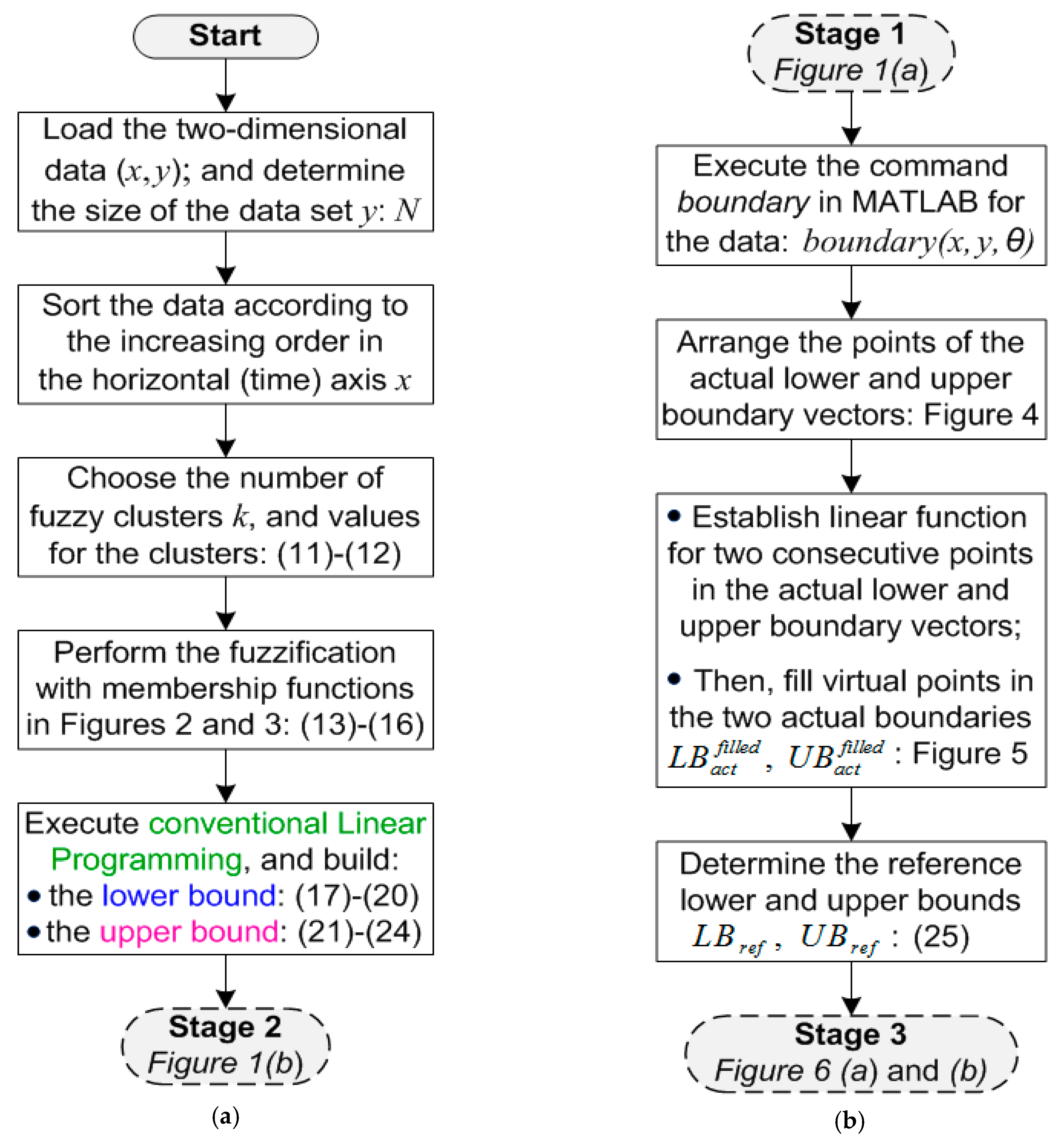
Figure 2.
The particular fuzzy clusters (membership functions) used in this research, where k = 24.
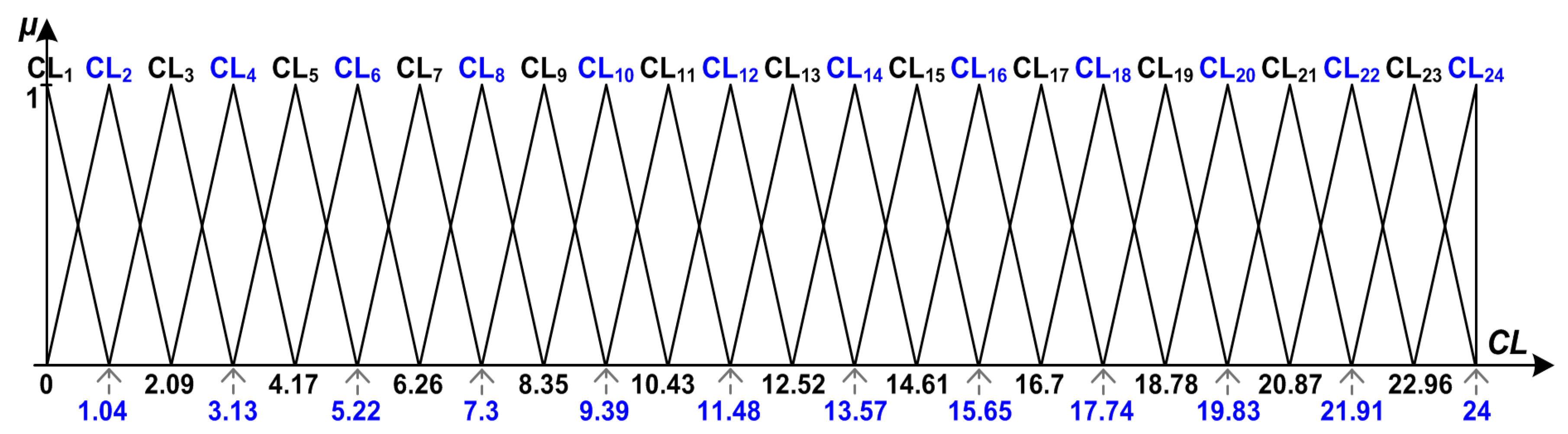
Figure 3.
(a) R-function fuzzy membership function, where = min(x); (b) Normal triangle fuzzy membership function; (c) L-function fuzzy membership function, where = max(x).
Figure 3.
(a) R-function fuzzy membership function, where = min(x); (b) Normal triangle fuzzy membership function; (c) L-function fuzzy membership function, where = max(x).

Figure 4.
The index vector of actual boundary data points using the MATLAB boundary command.
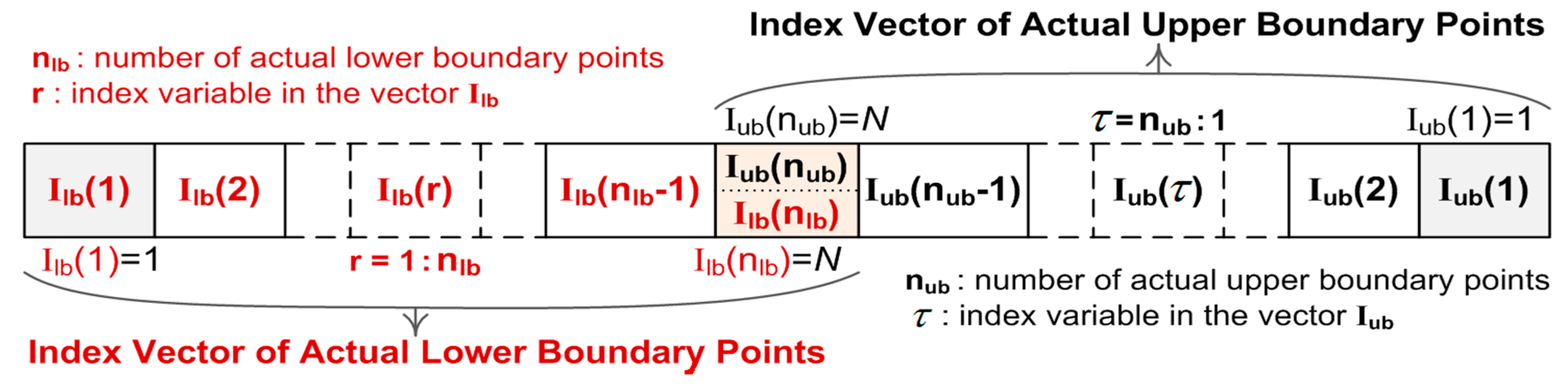
Figure 5.
Sample performance of the coIFML, and filled actual boundaries and using the syntax boundary(x, y, 0.73) in MATLAB for battery power data.
Figure 5.
Sample performance of the coIFML, and filled actual boundaries and using the syntax boundary(x, y, 0.73) in MATLAB for battery power data.

Figure 6.
(a) The third design stage for the lower bound of the proposed imIFML technique. (b) The third design stage for the upper bound of the proposed imIFML technique.
Figure 6.
(a) The third design stage for the lower bound of the proposed imIFML technique. (b) The third design stage for the upper bound of the proposed imIFML technique.

Figure 7.
(a) The fourth design stage for the lower bound of the proposed imIFML; (b) The fourth design stage for the upper bound of the proposed imIFML.
Figure 7.
(a) The fourth design stage for the lower bound of the proposed imIFML; (b) The fourth design stage for the upper bound of the proposed imIFML.
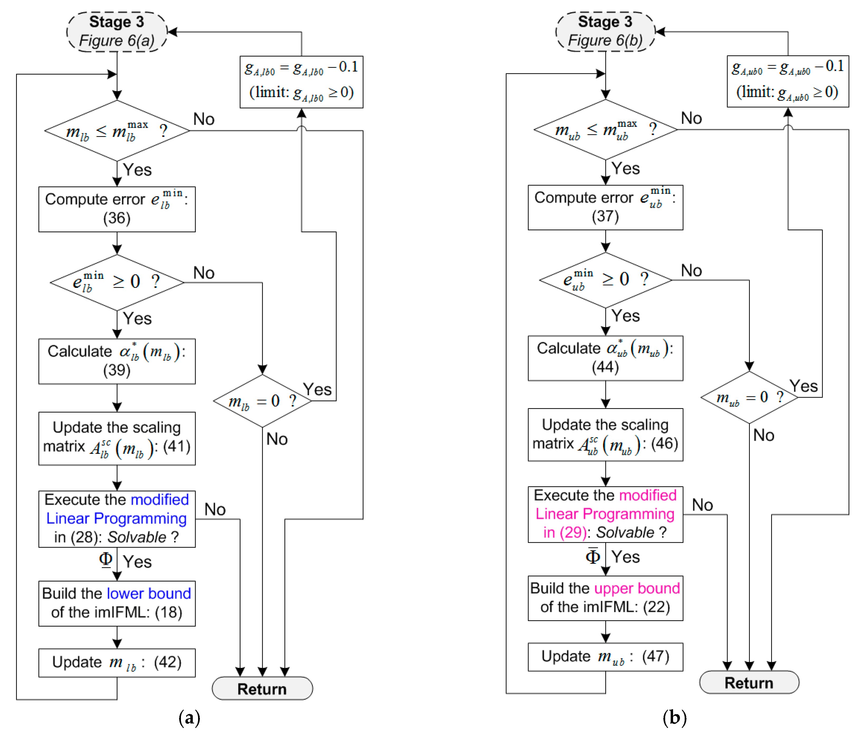
Figure 8.
The robust energy management system with the proposed imIFML for estimating solar PV, wind and battery power in a demonstrative renewable energy system.
Figure 8.
The robust energy management system with the proposed imIFML for estimating solar PV, wind and battery power in a demonstrative renewable energy system.
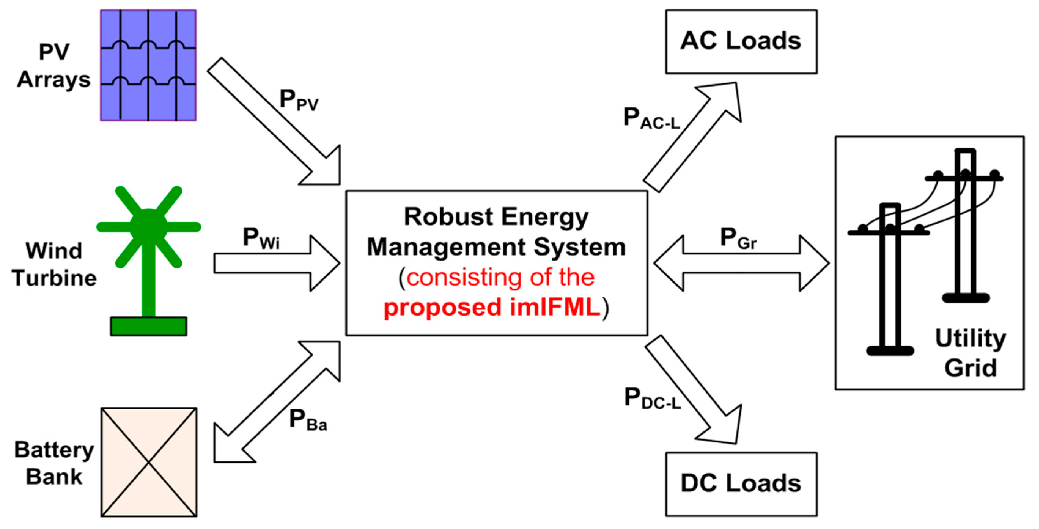
Figure 9.
Test case 1: Results of estimating battery power under the proposed imIFML technique.

Figure 10.
Test case 2: Results on estimating solar PV power under the proposed imIFML.
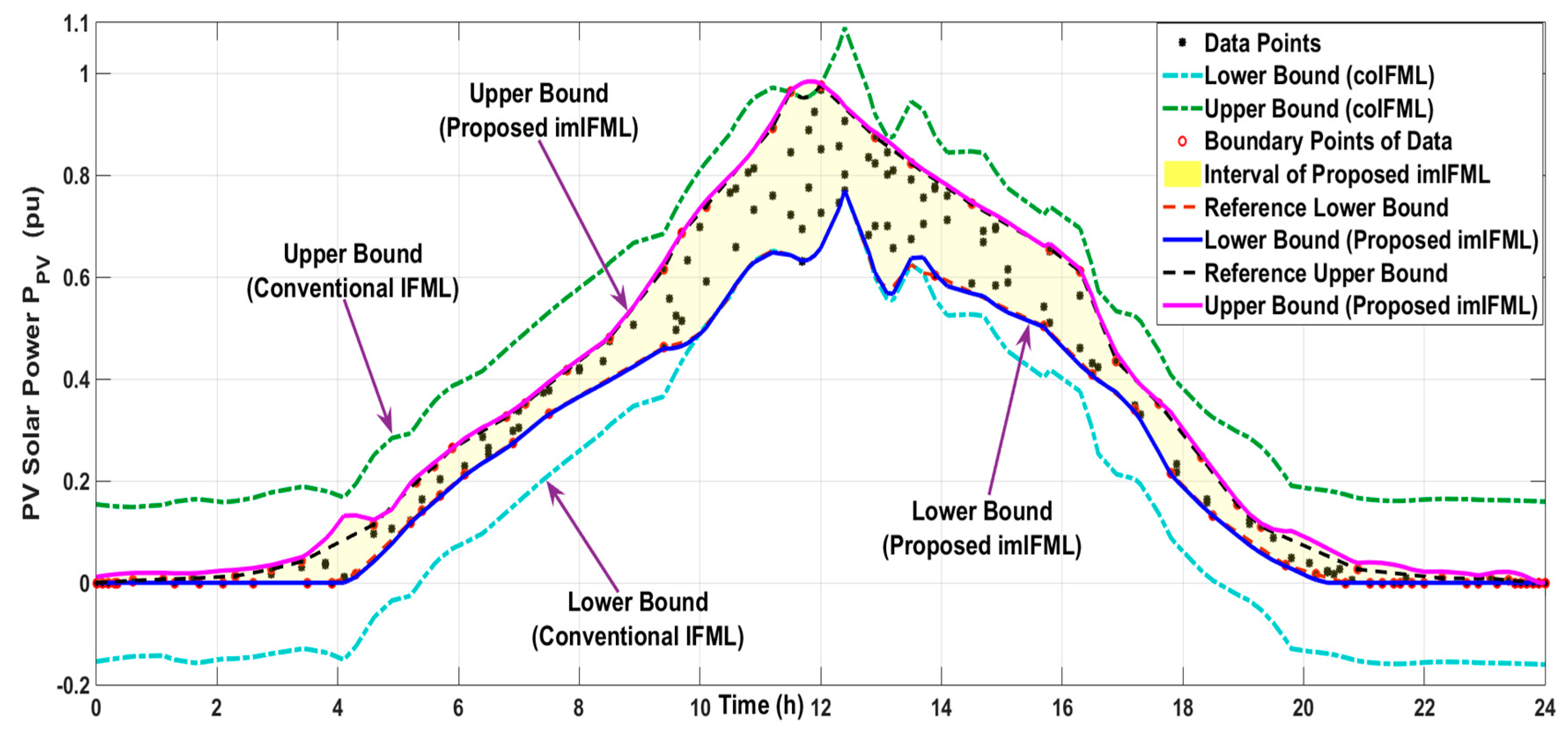
Figure 11.
Test case 3: Results on estimating wind power under the proposed imIFML.

© 2018 by the authors. Licensee MDPI, Basel, Switzerland. This article is an open access article distributed under the terms and conditions of the Creative Commons Attribution (CC BY) license (http://creativecommons.org/licenses/by/4.0/).
Share and Cite
MDPI and ACS Style
Thao, N.G.M.; Uchida, K. An Improved Interval Fuzzy Modeling Method: Applications to the Estimation of Photovoltaic/Wind/Battery Power in Renewable Energy Systems. Energies 2018, 11, 482. https://doi.org/10.3390/en11030482
AMA Style
Thao NGM, Uchida K. An Improved Interval Fuzzy Modeling Method: Applications to the Estimation of Photovoltaic/Wind/Battery Power in Renewable Energy Systems. Energies. 2018; 11(3):482. https://doi.org/10.3390/en11030482
Chicago/Turabian StyleThao, Nguyen Gia Minh, and Kenko Uchida. 2018. "An Improved Interval Fuzzy Modeling Method: Applications to the Estimation of Photovoltaic/Wind/Battery Power in Renewable Energy Systems" Energies 11, no. 3: 482. https://doi.org/10.3390/en11030482
Note that from the first issue of 2016, this journal uses article numbers instead of page numbers. See further details here.