A Soft Curtailment of Wide-Area Central Air Conditioning Load


1
Department of Electrical Engineering, National Taipei University of Technology, Taipei 10608, Taiwan
2
Faculty of Engineering, Technology and Built Environment, UCSI University, Kuala Lumpur 56000, Malaysia
*
Author to whom correspondence should be addressed.
Energies 2018, 11(3), 492; https://doi.org/10.3390/en11030492
Submission received: 26 January 2018
/
Revised: 19 February 2018
/
Accepted: 22 February 2018
/
Published: 26 February 2018
(This article belongs to the Section F: Electrical Engineering)
Abstract
:An innovative solution to provide a demand response for power system is proposed in this paper by considering the feasibility of two-way direct load control (TWDLC) of central air conditioning chiller system for wide-area in real-time manner. Particularly, the proposed TWDLC scheme is designed to tackle the load shedding ratio optimization problem for all under-controlled customers, aiming to satisfy the target load curtailment defined in each scheduling step. Another notable contribution of this work is the utilization of constraint loosening concept on actual load, curtailed to overcome the uncertainties of load reduction during TWDLC. Given the presence of fuzzy constraints, the proposed load shedding ratio optimization problem can be tackled using fuzzy linear programming. A delicate strategy is then formulated to transform the proposed fuzzy linear programming problem into a regular linear programming problem. A selection scheme used to obtain the feasible candidates set for load shedding at every sampling interval of TWDLC is also designed along with the fuzzy linear programming.
1. Introduction
The rapid development of smart grid [1,2,3], integrated with advanced metering infrastructure (AMI) and two-way communication capability offers a new opportunity for utility company to revolutionize the existing electrical systems. The emergence of these cyber-infrastructures allows for utility to exploit demand side capability of electricity users in order to achieve certain grid-level operation objectives, such as the reduction of peak demand and forced outage [4]. Utilities tend to deploy different demand response (DR) programs to fully realize the benefits of smart grid. On one hand, DR programs are considered by the electric system planners or utility operators as resource options to achieve electricity supply and demand balance. On the other hands, DR programs allow for the electricity user to have more active participation in the demand side of electric grid by reducing or shifting their electricity consumption during the peak periods. Existing DR programs are categorized into two types, namely the price-based and incentive-based schemes [5,6]. For latter schemes, electricity users are incentivized by utility or curtail service provider (CSP) for being able to reduce their energy consumption for a certain periods of time upon request.
Direct load control (DLC) is one common incentive-based DR program that is used by utility or CSP to reshape load profile by scheduling the operation cycles of customer’s high-power appliances. Central air conditioning chillers of industrial and commercial customers are the excellent candidates to achieve a cost effective DLC because the potential load reduction capacity delivered can reach up to several hundred kilowatts. Given the impressive strides that have been made in metering and intelligent control technologies in facilitating a continuous bidirectional communication between the utility or CSP and its customers [7,8], a two-way direct load control (TWDLC) scheme for central air-conditioning chiller systems can further be envisioned as an emergency demand response mechanism with real-time load shedding effect. In particular, the utility or CSP can transmit the load shedding signals to its controlled customers, while monitoring the load shedding results continuously via the Internet. The TWDLC of central chillers can even serve as an ancillary service if a huge amount of central chiller loads are aggregated, monitored, and managed effectively under smart grid environment [9,10]. A successful load shedding program can reduce the cost of electricity in wholesale market and this leads to lower electricity retail prices. Furthermore, these load shedding programs also have the potential to help a utility company in achieving cost saving via peak demand reductions and defer the necessity of constructing the new power plants that reserved for use during peak times.
Computational intelligence approach has gained popularity in recent years to solve complex DLC scheduling problems. An iterative deepening search strategy was incorporated into genetic algorithm [11] and genetic programming [12] to produce a DLC schedule of air conditioning load that is capable of meeting the target load shed profile with minimum cost. A DLC scheduling problem with multiobjective framework was solved from different perspectives using an interactive evolutionary algorithm [13,14]. An optimal DLC dispatch of air-conditioning loads was proposed in [15] using an imperialist competitive algorithm to optimize the actual target load shed profile to ensure that it can be as close as possible to the predefined target profile. An innovative modelling of DLC for air-conditioning loads was coordinated along with unit commitment in [16] using distributed imperialist competitive algorithm to minimize system operational cost. In [17], the operational cost of a micro-grid with high penetration of solar power and air conditioning loads was successfully minimized by using the differential evolution. A hierarchical DLC framework for large-scale air conditioning load dispatch was proposed in [18] using differential evolution algorithm to minimize the operational cost. With a two-way communication platform, the load curtailment of central air-conditioning systems can be achieved in real-time using linear programming [19]. By considering the uncertainties of electricity prices and ambient temperature change, a DLC of air-conditioning loads was solved in [20] by mixed-integer linear programming to enhance wind power utilization level and minimize the system operational cost. By considering the transmission system reliability, an optimal DLC schedule of air conditioning loads was obtained in [21] by a fuzzy DR to attain a tradeoff between peak load and system operation cost reduction. In [22], a nonlinear programming approach was formulated by considering DLC as a part of integrated resource planning to minimize the investment cost of a microgrid. A DLC union was formed for the retailer and residential users in [23] using cooperative game to minimize the regulation cost of retailer by providing users an indirect access into balance market to improve market efficiency. A model estimator controller was designed in [24] using Markov chain model to coordinate aggregation of air-conditioning loads in order to address energy imbalance issue in power systems. Both of the distributed load shedding and micro-generator dispatching was coordinated in [25] using a probabilistic method to provide an emergency DR. A novel DLC scheme was proposed using queuing system model to control the air-conditioning loads without comprising users’ cooling comfort [26].
Most existing DLC scheduling strategies have not, to the authors’ best knowledge, considered the uncertainties of demand reduction provided by air-conditioning loads. The previous works assumed the target load shed to be met are fixed and crisp optimization constraints were formulated to guarantee the actual curtailment produced does not violate the target profile. In practical scenarios, the load reduction that is produced by central chiller systems in large-scale geographical area is affected by different factors, including the ambient temperature, number of people in the cooling environment, communication network signal strength, etc. [27]. The optimality of DLC schedules produced without taking these uncertainties into account is hence questionable. The main contribution of this paper is to propose an innovative approach based on fuzzy linear programming [28] to tackle the TWDLC optimization of central chiller systems in greater flexibility manner. Particularly, a fuzzy inference system is designed to model the uncertainties of load reduction by allowing for a certain degree of constraint loosening to obtain an optimal TWDLC schedule of central chiller systems. With these optimization flexibilities, a soft curtailment for the TWDLC of central air conditioning systems is achieved. With the proposed approach, a tolerance range of load reduction uncertainty is provided to the aggregators as they negotiate DR capacity and purchase prices with CSPs [29,30].
The rest of this paper is organized as follows. In Section 2, the problem formulation for TWDLC of central air-conditioning chiller systems are described. An optimization approach used to determine the best set of candidates for load curtailment throughout the control intervals is then explained in Section 3. The implementation of fuzzy linear programming for TWDLC is described in Section 4. Extensive simulation studies used to verify the performance of the proposed scheduling optimization approach are demonstrated in Section 5. Finally, some concluding remarks are drawn in Section 6.
2. Problem Formulation for TWDLC of Central Chiller
Consider that a total of N customers are recruited by utility company or CSP to participate the TWDLC program and Ci chillers at every i-th customers are under control, i = 1, …, N. In this study, a scheduling optimization scheme is formulated to achieve TWDLC of central chiller systems in real-time. At any time period t, let the operational status of the j-th central chiller unit belonging to the building of i-th customer be denoted as . The running status of the j-th chiller owned by the i-th customer is assigned as = 1 if it is turned on during time period t and = 0 for otherwise, j = 1, …, Ci, i = 1, …, N. From technical point of view, the load curtailment for a centrifugal compressor can be achieved through partial load reduction instead of turning the equipment off. Chiller energy efficiency is measured using the coefficient of performance (COP), which varies with chiller’s load ratio. It is noteworthy that the majority of central chillers suffers with drastic COP drops when its load ratio is 50% or lesser, leading to poor energy efficiency. In order to prevent the chiller from having undesirably low COP due to the partial load reduction for DLC, it is necessary to define the lower boundary of chiller’s load ratio. Denote and as chiller’s capacity and the load measured at time t, respectively, and as the lower bound of the load ratio for the j-th chiller of the i-th customer. Let be the controllable load available for each i-th customer and it refers to the total controllable load among all of the chillers belonging to that customer, i.e.,:
where the controllable load for the j-th chiller of the i-th customer is defined as:
For customers that are willing to participate in the curtailed service program or similar DR programs, a set of load management facility consisting of gateway and chiller control network will be installed into their buildings by the utility company or curtailed service provider. Once the load curtailment signal is received by gateway through the Internet over the broadband network from the control center at time t, the gateway needs to determine the required load curtailment for each central chiller, followed by the activation of load curtailment through the chiller control network. Define Tc as the overall control interval of TWDLC, while Ts refers to the sampling interval that is set by the control center to perform TWDLC. Then, the total number of evaluations throughout the entire control interval of TWDLC is defined as .
The computer server in control center reviews available customers for load control during the k-th scheduling step , k = 1, …, M. As long as the customer is available for control, the average controllable load is measured at every sampling interval. Denote as the average controllable load for the i-th available customer at and as the averaging interval for calculating . Then,
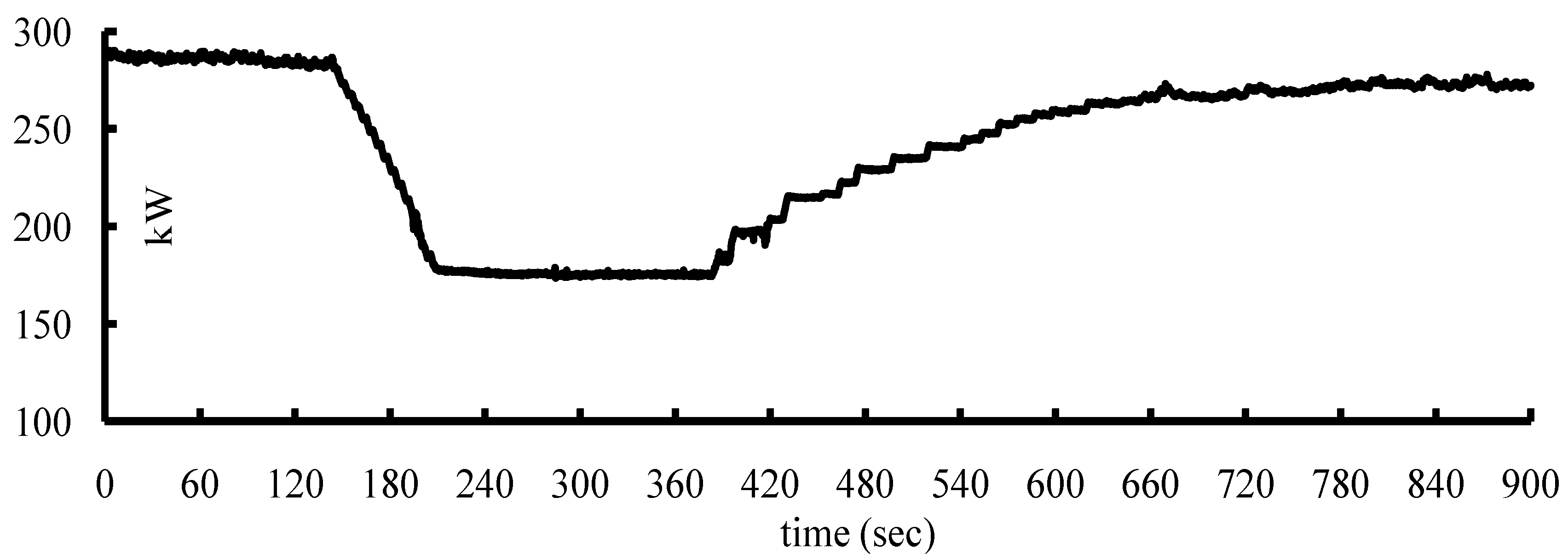
As soon as reviewing all of the available customers for control, the computer server in control center selects certain number of available customers for load shedding by sending out load shedding commands through the Internet to the gateway at customer site. Figure 1 shows the load variation of a typical chiller starts shedding load to a certain ratio, maintains the load ratio for certain period of time and restores the load back to the original load before shedding. It is shown in Figure 1 that a period of time is required for a chiller to conduct load shedding and load restoration. For customers that are chosen for load shedding, the actual load reduction delivered by a chiller is measured by gateway and reverted to computer server in control center through internet. Denote as the average load after load shedding for the i-th available customer and as the time interval to wait until the chiller finishes load shedding. Then,
With the average loads defined in (3) and (4), the average shed load is defined as:
The average controllable load available for each under-controlled customer,, i = 1, …, N, at each scheduling step is measured and revert to control center through the Internet by the gateway installed at customer’s site. A real-time optimization scheme is then formulated in this paper for determining the combination of load shedding ratios for all of the customers at every time step through the entire control interval based on the received average controllable load , i = 1, …, N. Let be the expected load shedding ratio computed by the computer server in control center for each i-th customer. The calculated load shedding ratio is defined as the ratio of expected load curtailed with respect to average controllable load of customer i. The proposed optimization approach aims to find the best combination of load shedding ratio of each central chiller unit in real time so that the overall target shed load is individually satisfied at every scheduling period. The overall target shed load is the total load that is required to curtail by the direct control of entire set of central chillers.
Denote P(·) as the overall target shed load based on the load forecast, while J(·) is a set consisting of all customers available for TWDLC. The utility aims to minimize the load curtailment produced by TWDLC in order to minimize utility’s electricity sale loss while satisfy overall and regional target shed load. When considering that the target shed load is derived by referring to load forecast, it is necessary to facilitate certain degree of precision tolerance corresponds to weather, temperature, control timing, customer conditions, etc. Particularly, the constraint for the calculated shed load to be greater than the overall target load curtailment allows for a certain degree of loosening. With this constraint loosening, more calculation flexibility is allocated to tackle the TWDLC scheduling optimization using fuzzy linear programming. The fuzzy linear programming categorized as linear programming with fuzzy resources is defined as:
subject to
and
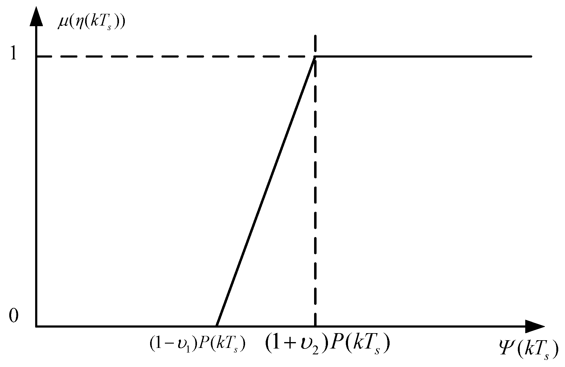
The expected shedding ratios range between 0 and 1. However, if the calculated is too small, then the required shed load at the corresponding customer might be barely greater than the disturbance, leading to insignificant shedding contribution to the entire load reduction. Even though some of the calculated shedding ratios are insignificantly small, the control center still needs to send these ratios one by one to the corresponding gateways at customer sites, leading to inefficient communication efforts. To avoid obtaining insignificantly small values, a lower bound is assigned to the shedding ratio. Therefore, the calculated shedding ratio in the optimization is constrained between 0.1 and 1, as in (7). The sign “” in (8) symbolizes that the inequality is in essence with fuzziness. The load curtailment due to TWDLC in (8) could be considered as a soft curtailment because the load shed quantity is allowed to vary within a soft range. The fuzzy constraint of (8) is described by the membership function , as illustrated in Figure 2, where the tolerance for the fuzzy constraint is represented using two coefficients . Denote as the calculated shed load, that is,
Mathematically, the fuzzy constraint described by the membership function in Figure 2 is given as:
3. Mechanism of Candidates Selection for TWDLC
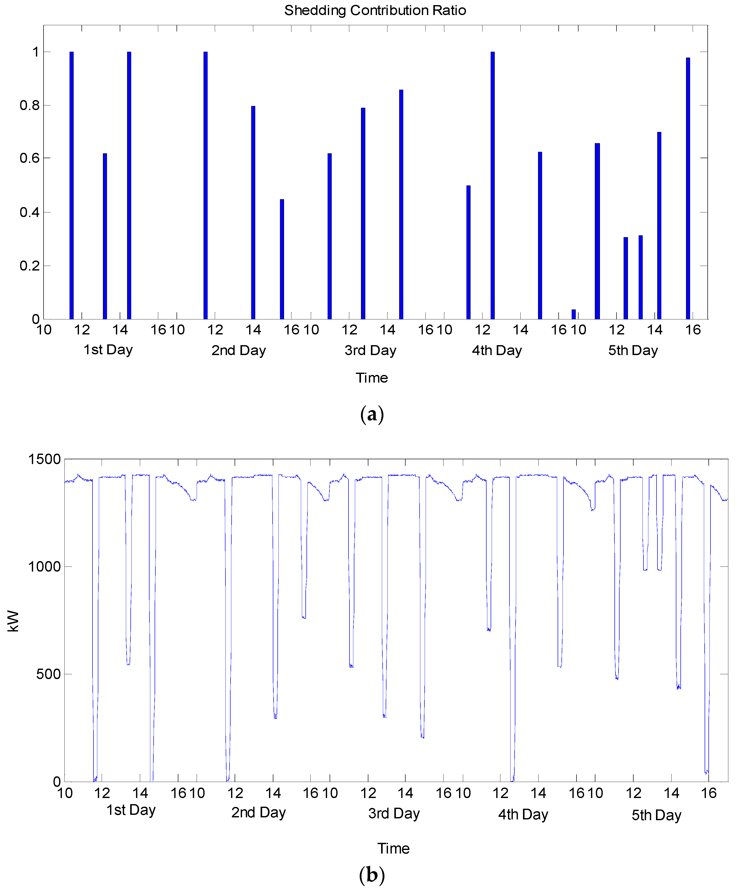
The monitoring and control of every chiller for the computer server is achieved through the gateway installed at the building of each customer. To ease the computational and communication effort, the computer server calculates the load to be curtailed and sends the shedding control commands in customer by customer basis instead of in chiller by chiller basis. The customer determination for shedding at each scheduling step is to fulfill the target shedding capacity P(·) and to level off the contribution to the entire load shedding for every customer. A coefficient denoted as is introduced as shedding contribution ratio to measure the load curtailment contributed by each i-th customers. Mathematically, is defined as a ratio between the average actual curtailed load to the average controllable load as follows:
For each customer, the respective accumulated time of under-controlled status is recorded by the computer server. This information is considered as one of the reference indices to select the customer for load shedding at every scheduling period. Let and be the effective accumulated time of under-controlled and off-controlled status for each i-th customer up to the k-th scheduling step, respectively. Practically, these effective accumulated times can be calculated by adding up the time intervals of under-controlled and off-controlled status for each i-th customer. The shedding contribution ratios are also taken into account. For instance, the customers assigned with higher shedding contribution ratios tend to experience more cooling comfort losses than those with lower shedding contribution ratios. Therefore, the effective increments of the accumulated times under control are considered to be longer than the ones for customers with lower shedding contribution ratios. An adjustment scheme for the accumulated time under control and off control is then proposed by referring to the previous experience of load shedding control as well as the feedback collected from customers. Accordingly, no adjustment is needed for the customers with shedding contribution ratios greater than 0.75. For the customer with smaller than 0.15, the associated equivalent shedding intervals are reduced to 1/3 in order to reflect the lesser loss of cooling comfort experienced by these customers during of shedding control period of TWDLC. As for the customers with fall between 0.15 and 0.75, a linear function is formulated to adjust their equivalent shedding intervals between 1/3 to 1, based on . Denote as the adjustment coefficient of each i-th customer, then:
Let be a binary variable indicates the control status of every i-th customer during the k-th scheduling step. Specifically, is assigned for the under-controlled costumers, while is assigned for those either in off-controlled status or just restored from being controlled. and are effectively adjusted with reference to as follows:
∀i = 1, …, N and k = 1, …, M, where and .
Notably, the variable shown in both (13) and (14) is the complement of . It is also shown in (13) and (14) that the variables and are reset to zero once the control status changes. From (12) to (14), customers with larger in the previous scheduling period have effectively more accumulated and vice versa. The accumulated time under control needs an upper limit in order not to affect too much cooling comfort due to load shedding. Denote as the maximum allowable time for the i-th customer to perform continuous shedding control, then:
For a customer with off-controlled status, it means that the customer is restored from the previous shedding control. It takes time for the building to regain cooling comfort before it is controlled again. Let be the least time the i-th customer needs to stay off-controlled, then
Every i-th customer becomes a candidate for load shedding if both constraints in (15) and (16) are satisfied. On the contrary, if the constraint in either (15) or (16) is violated, the i-th customer is removed from the candidate list for load curtailment in the next scheduling period. Therefore,
Every customer’s shedding contribution ratio is accumulated and recorded in the computer server at the control center. Let and represent the accumulated shedding contribution ratio and its average value, respectively, for the i-th customer building at the k-th time step, then
where the initial value . As the TWDLC is conducted day by day, the load shedding control fairness needs to be watched because it is a long-term change in cooling comforts for customers. The computer server in the control center monitors and compares the accumulated shedding contribution of each customer with the average contribution among all of the customers to avoid certain customers from being controlled too frequent and lead to the biasing of load shedding fairness. For the i-th customer, if , the customer can be removed from the candidate list for load curtailment in the next scheduling period. Therefore,
Conversely, if , it is expected that more contribution to the TWDLC is required and the customer is taken as a candidate for load curtailment. Let be the set of candidates available for load curtailment at the -th scheduling period based on the records calculated up to the k-th scheduling period. Referring to (15), (16), and (20), is defined as:
Referring to (6), a set consisting of optimization decision variables denoted as J(·), is shown in (21).
4. Fuzzy Linear Programming
The optimization in (6) with of the crisp constraint (7) and the fuzzy constraint (8) described by the membership function in (10), can be addressed by first converting it into two standard linear programming problems shown, as follows:
where v1 and v2 are defined in the membership function in (8). Assume that the optimal solution of (19) and (20) are and , respectively. Denote the shed load corresponding to and as and , respectively, i.e.,
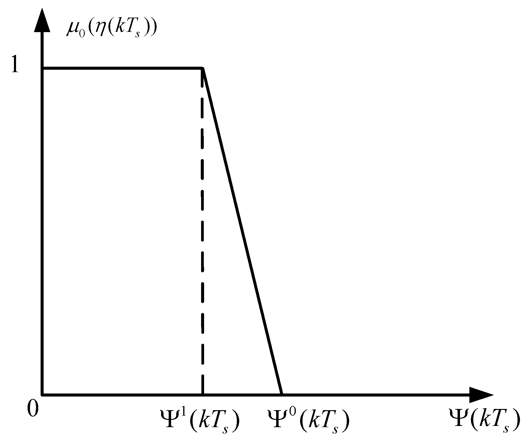
The degree of optimality is described using the following membership function illusrated in Figure 3 based on and as following:
Given that the fuzzy constraint is converted into the membership function μ in (10) and the objective function associated with the fuzzy constraint is converted into the membership function in (26), the max-min approach can then be used to solve the optimization in (6)–(8), as follows:
Without loss of generality, the constrained max-min optimization problem described in (27) can be rewritten into standard linear programming problem as follow:
where , .
Substituting (26) into (30) to produce an equivalent constraint of (30) known as:
Similarly, substituting (10) into (31), to produce an equivalent constraint of (31) known as:
Note that the constraint in (29) is not in expressed as the standard format of linear programming. To overcome this issue, the surplus decision variable of for is first defined, followed by a large constant of Q >> 1. To this end, the constraint in (29) can be expressed in the standard format of:
Therefore, the fuzzy linear programming in (6)–(8) can be easily addressed by solving the equivalent linear programming problem in (28) with constraints in (32)–(35).
5. Computer Simulation
A total of 30 customers are selected in this section to evaluate the load shedding performance of the proposed TWDLC algorithm using fuzzy linear programming. The overall load shedding was conducted for five consecutive days, started from 10:00 to 17:00 each day. The sampling interval of computer server to retrieve the controllable load of every customer and to conduct load curtailment through gateway are both set as Ts = 15 min, as recommended by most previous studies, such as those in [11,12,19,20,22,26]. The averaging interval Tm in (3) and the waiting interval Tw in (4) for the gateway to calculate the average controllable load before and after every sampling time are both set as three minutes. Other simulation parameters including the actual capacity, maximum controllable load and the time constraints to remain under-controlled and off-controlled status for each customer throughout five consecutive days of load shedding are provided in Table 1.
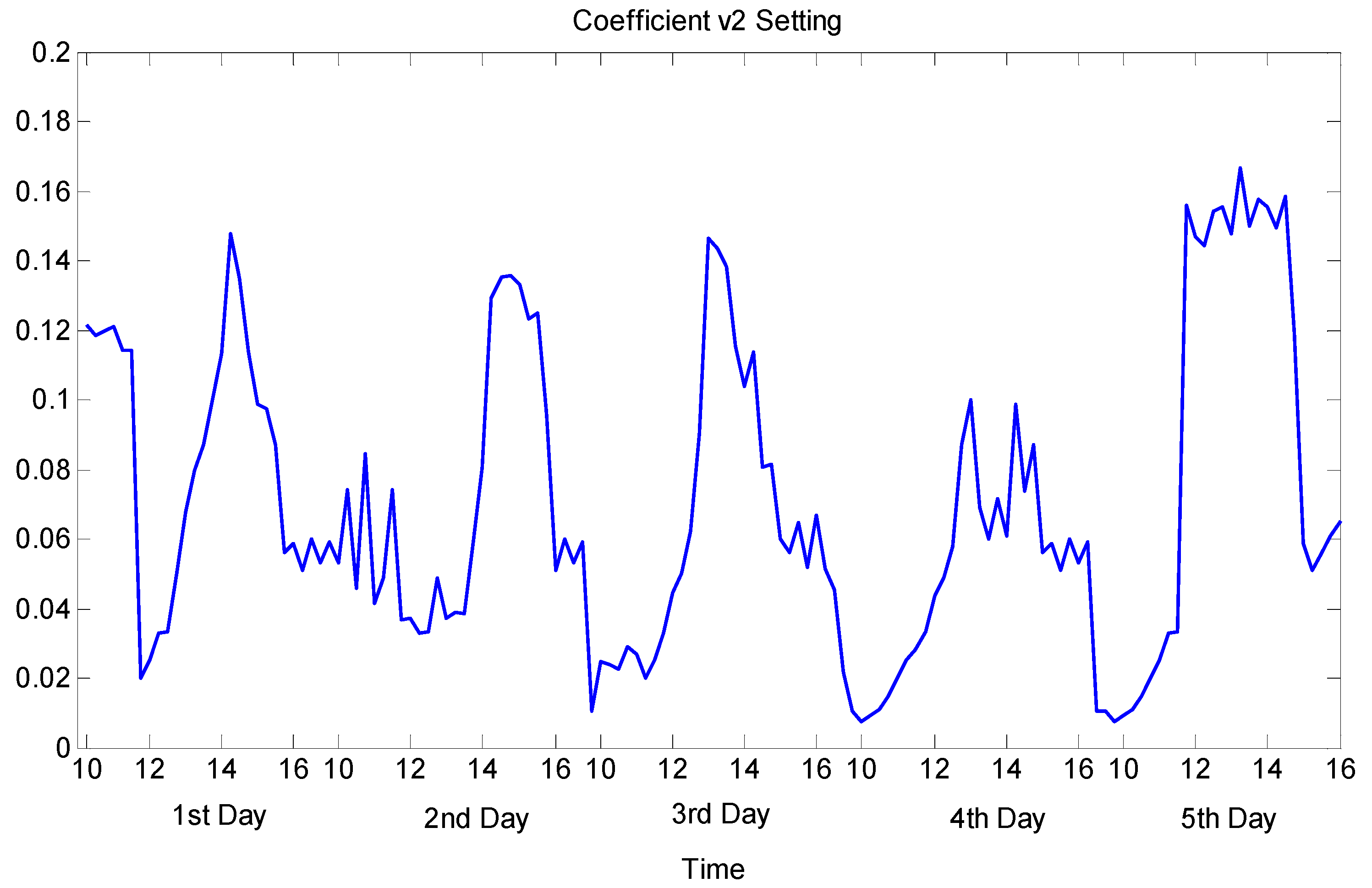
Recall that v1 and v2 in association with the membership function in (10) represent the fuzzy constraint in (8) that the calculated load shed greater than or equal to the target load P(·) to a certain degree of precision tolerance. Both coefficients v1 and v2 could be either constants or time-varying functions since the degree of precision tolerance for the fuzzy constraint in (8) can vary with the temperature, load in regional power system, or time of a day, etc. In this paper, the variations of v1 and v2 are both set as time-varying functions, as shown in Figure 4 and Figure 5, respectively. Using the proposed optimal real-time scheduling approach based on fuzzy linear programming, the calculated load shed, , is illustrated in Figure 6. Both of the upper and lower boundaries of fuzzy constraints in (8), denoted as and , respectively, as well as the target load shedding profile are also compared with in Figure 6. In Figure 6, it is shown that the optimized load shed matches the target load well in response to the variations in target load tolerance. Meanwhile, Figure 7a,b illustrate the optimized shedding ratios and the controllable load of customer with the largest capacity.
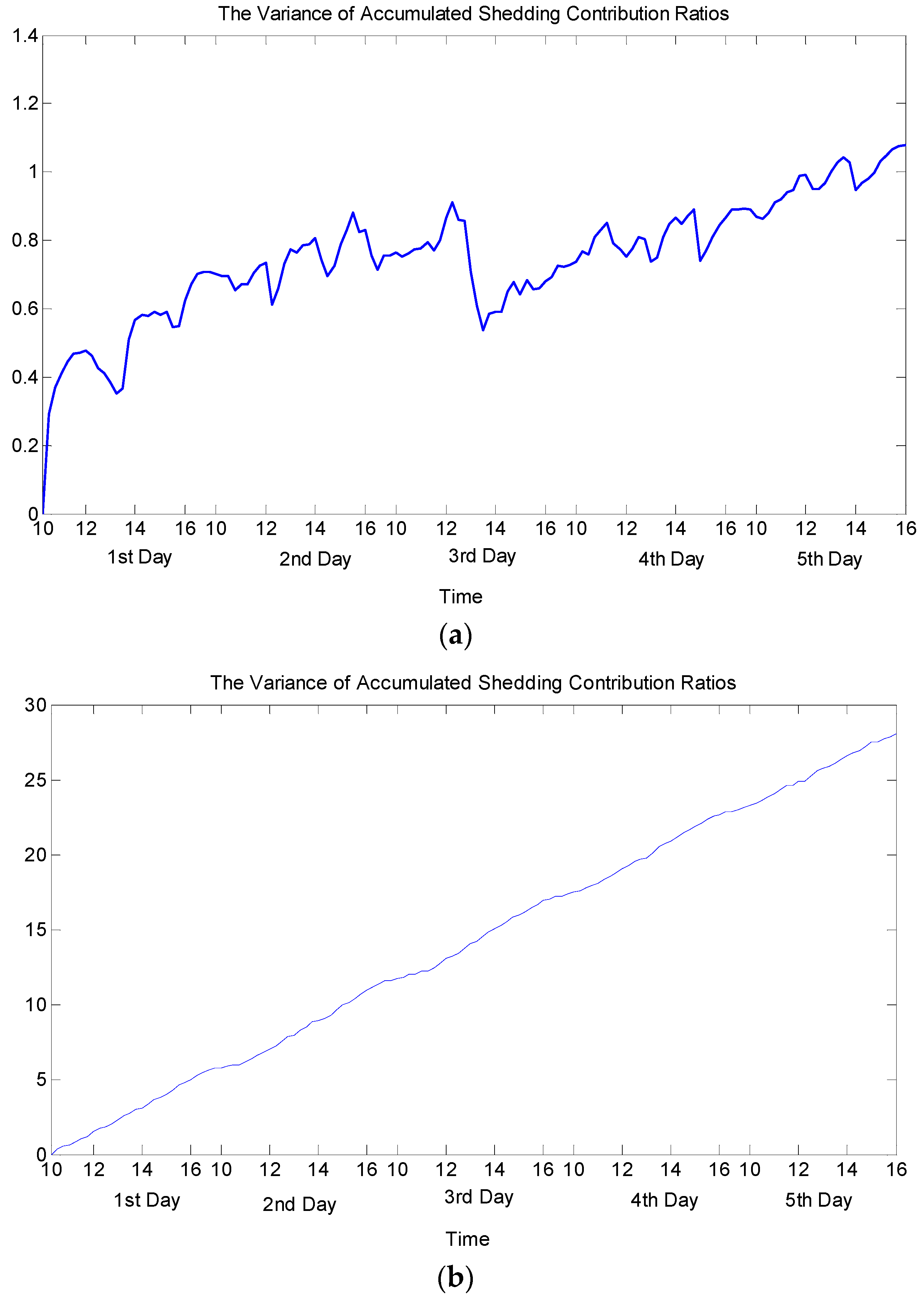
Different customers are assigned with different shedding times as well as load shedding ratios due to different capacity and time constrains assigned. In order to show the effectiveness of the filtering scheme defined in (20), a metric used to consider the standard deviation ofs accumulated shedding contribution ratios at every k-th scheduling step is formulated as:
Note that the accumulated shedding contribution ratio of the i-th customer is defined in (18), while the average accumulated shedding contribution ratio can be obtained from (19). The variation profiles of with and without the filtering scheme in (20) are both shown in Figure 8a,b, respectively. From Figure 8a, it is observed that the variation of accumulated shedding contribution ratios is relatively insignificant as times goes on when the filtering scheme in (20) is applied. This shows that the filtering scheme levels off the contribution of each customer that is participating in load shedding, hence guaranteeing the load shedding fairness. Conversely, if the filtering scheme in (20) is removed from the customer selection process, Figure 8b illustrates that the accumulated shedding contribution ratios tend to increased drastically with time.
6. Conclusions
A real-time two-way direct lad control (TWDLC) optimization scheme is proposed as an effective demand response approach by scheduling the load shedding of the central air-conditioning chiller systems in wide area. The proposed TWDLC works well through the broadband network with gateway installed at the building of every customer. Fuzzy linear programming is utilized to solve the DLC optimization in more flexible manner because it allows for a certain degree of precision tolerance for shed load constraints. It is shown in simulation that the load shedding performance delivered by the proposed TWDLC scheme is promising, hence feasible for real-time optimization and time-varying precision tolerance in response to variable target load profile.
For future work, the degree of precision tolerance for the fuzzy constraints can be linked with weather condition, regional load, time of a day, etc., depending on the application scenario. Delicate modeling can be designed to automatically adjust the precision tolerance in response to environmental changes. Type-2 membership functions can also be used to define precision tolerance of constraints for future work.
Author Contributions
Leehter Yao conceived and designed the main ideas proposed in the paper. He also wrote the paper. Lei Yao designed and performed the experiments. Wei Hong Lim designed the fuzzy linear programming model and analyzed the data.
Conflicts of Interest
The authors declare no conflict of interest.
References
- Rahimi, F.; Ipakchi, A. Demand response as a market resource under the smart grid paradigm. IEEE Trans. Smart Grid 2010, 1, 82–88. [Google Scholar] [CrossRef]
- Medina, J.; Muller, N.; Roytelman, I. Demand response and distribution grid operations: Opportunities and challenges. IEEE Trans. Smart Grid 2010, 1, 193–198. [Google Scholar] [CrossRef]
- Varaiya, P.P.; Wu, F.F.; Bialek, J.W. Smart operation of smart grid: Risk-limiting dispatch. IEEE Proc. 2011, 99, 40–57. [Google Scholar] [CrossRef]
- Pullins, S.; Westerman, J. San Diego Smart Grid Study Final Report; Technical Report; Science Applications Int. Corp.: Reston, VA, USA, October 2006. [Google Scholar]
- Albadi, M.H.; El-Saadany, E.F. Demand response in electricity markets: An overview. In Proceedings of the IEEE PES General Meeting, Tampa, FL, USA, 24–28 June 2007; pp. 1–5. [Google Scholar]
- U.S. Department of Energy. Benefits of Demand Response in Electricity Markets and Recommendations for Achieving Them; Report to the United State Congress; February 2006. Available online: http://eetd.lbl.gov (accessed on 7 January 2018).
- Reusens, P.; Bruyssel, D.V.; Sevenhans, J.; Bergh, S.V.D.; Nimmen, B.V.; Spruyt, P. A practical ADSL technology following a decade of effort. IEEE Commun. Mag. 2001, 39, 145–151. [Google Scholar] [CrossRef]
- Ouyang, F.; Duvaut, P.; Moreno, O.; Pierrugues, L. The first step of long-reach ADSL: Smart DSL technology, READSL. IEEE Commun. Mag. 2003, 41, 124–131. [Google Scholar] [CrossRef]
- Parvania, M.; Fotuhi-Firuzabad, M. Demand response scheduling by stochastic SCUC. IEEE Trans. Smart Grid 2010, 1, 89–98. [Google Scholar] [CrossRef]
- Brooks, A.; Lu, E.; Reicher, D.; Spirakis, C.; Weihl, B. Demand dispatch. IEEE Power Energy Mag. 2010, 8, 20–29. [Google Scholar] [CrossRef]
- Yao, L.; Chang, W.-C.; Yen, R.-L. An iterative deepening genetic algorithm for scheduling of direct load control. IEEE Trans. Power Syst. 2005, 20, 1414–1421. [Google Scholar] [CrossRef]
- Yao, L.; Chou, Y.-C.; Lin, C.-C. Scheduling of direct load control using genetic programming. Int. J. Innov. Comput. I 2011, 7, 2515–2528. [Google Scholar]
- Gomes, A.; Antunes, C.H.; Martins, A.G. A multiple objective approach to direct load control using an interactive evolutionary algorithm. IEEE Trans. Power Syst. 2007, 22, 1004–1011. [Google Scholar] [CrossRef]
- Gomes, A.; Antunes, C.; Oliveira, E. Direct load control in the perspective of an electricity retailer—A multi-objective evolutionary approach. In Soft Computing in Industrial Applications; Springer: Berlin/Heidelberg, Germany, April 2011; pp. 13–26. [Google Scholar]
- Luo, F.; Zhao, J.; Dong, Z.Y.; Tong, X.; Chen, Y.; Yang, H.; Zhang, H. Optimal dispatch of air conditioner loads in southern china region by direct load control. IEEE Trans. Smart Grid 2016, 7, 439–450. [Google Scholar] [CrossRef]
- Luo, F.; Zhao, J.; Wang, H.; Tong, X.; Chen, Y.; Dong, Z.Y. Direct load control by distributed imperialist competitive algorithm. J. Mod. Power Syst. Clean Energy 2014, 2, 385–395. [Google Scholar] [CrossRef]
- Luo, F.; Xu, Z.; Meng, K.; Dong, Z.Y. Optimal operation scheduling for microgrid with high penetrations of solar power and thermostatically controlled loads. Sci. Technol. Built Environ. 2016, 22, 666–673. [Google Scholar] [CrossRef]
- Luo, F.; Dong, Z.Y.; Meng, K.; Wen, J.; Wang, H.; Zhao, J. An operational planning framework for large-scale thermostatically controlled load dispatch. IEEE Trans. Ind. Inform. 2017, 13, 217–227. [Google Scholar] [CrossRef]
- Yao, L.; Lu, H.-R. A two-way direct control of central air-conditioning load via Internet. IEEE Trans. Power Deliv. 2009, 24, 240–248. [Google Scholar] [CrossRef]
- Wang, D.; Meng, K.; Gao, X.; Coates, C.; Dong, Z. Optimal air-conditioning load control in distribution network with intermittent renewables. J. Mod. Power Syst. Clean Energy 2017, 5, 55–65. [Google Scholar] [CrossRef]
- Goel, L.; Wu, Q.; Wang, P. Fuzzy logic-based direct load control of air conditioning loads considering nodal reliability characteristics in restructured power system. Electr. Power Syst. Res. 2010, 80, 98–107. [Google Scholar] [CrossRef]
- Zhu, L.; Yan, Z.; Lee, W.-J.; Yang, X.; Fu, Y.; Cao, W. Direct load control in microgrids to enhance the performance of integrated resources planning. IEEE Trans. Ind. Appl. 2015, 51, 3553–3560. [Google Scholar] [CrossRef]
- Cui, Q.; Wang, X.; Wang, X.; Zhang, Y. Residential applicances direct load control in real-time using cooperative game. IEEE Trans. Power Syst. 2016, 31, 226–233. [Google Scholar] [CrossRef]
- Mathieu, J.L.; Koch, S.; Callaway, D.S. State estimation and control of electric loads to manage real-time energy imbalance. IEEE Trans. Power Syst. 2013, 28, 430–440. [Google Scholar] [CrossRef]
- Argiento, R.; Faranda, R.; Pievatolo, A.; Tironi, E. Distributed interruptible load shedding and micro-generator dispatching to benefit system operations. IEEE Trans. Power Syst. 2012, 27, 840–848. [Google Scholar] [CrossRef]
- Lee, S.C.; Kim, S.J.; Kim, S.H. Demand side management with air conditioner loads based on the queuing system model. IEEE Trans. Power Syst. 2011, 26, 661–668. [Google Scholar] [CrossRef]
- Sullivan, M.; Bode, J.; Kellow, B.; Woehleke, S.; Eto, J. Using residential AC load control in grid operations: PG&E’s ancillary service pilot. IEEE Trans. Smart Grid 2013, 4, 1162–1170. [Google Scholar]
- Wang, L.-X. A Course in Fuzzy Systems and Control; Pearson Education: London, UK, 2005. [Google Scholar]
- Nguyen, D.T.; Negnevitsky, M.; Groot, M.D. Walrasian market clearing for demand response exchange. IEEE Trans. Power Syst. 2012, 27, 535–544. [Google Scholar] [CrossRef]
- Gkatzikis, L.; Koutsopoulos, I.; Salonidis, T. The role of aggregators in smart grid demand response markets. IEEE J. Sel. Areas Commun. 2013, 31, 1247–1257. [Google Scholar] [CrossRef]
Figure 1.
Load variation as a typical chiller conducts load shedding and load restoration.

Figure 2.
Membership function used to describe the fuzzy constraint of (8).

Figure 3.
Membership function used to describe the degree of optimality.

Figure 4.
The variation of coefficient v1.
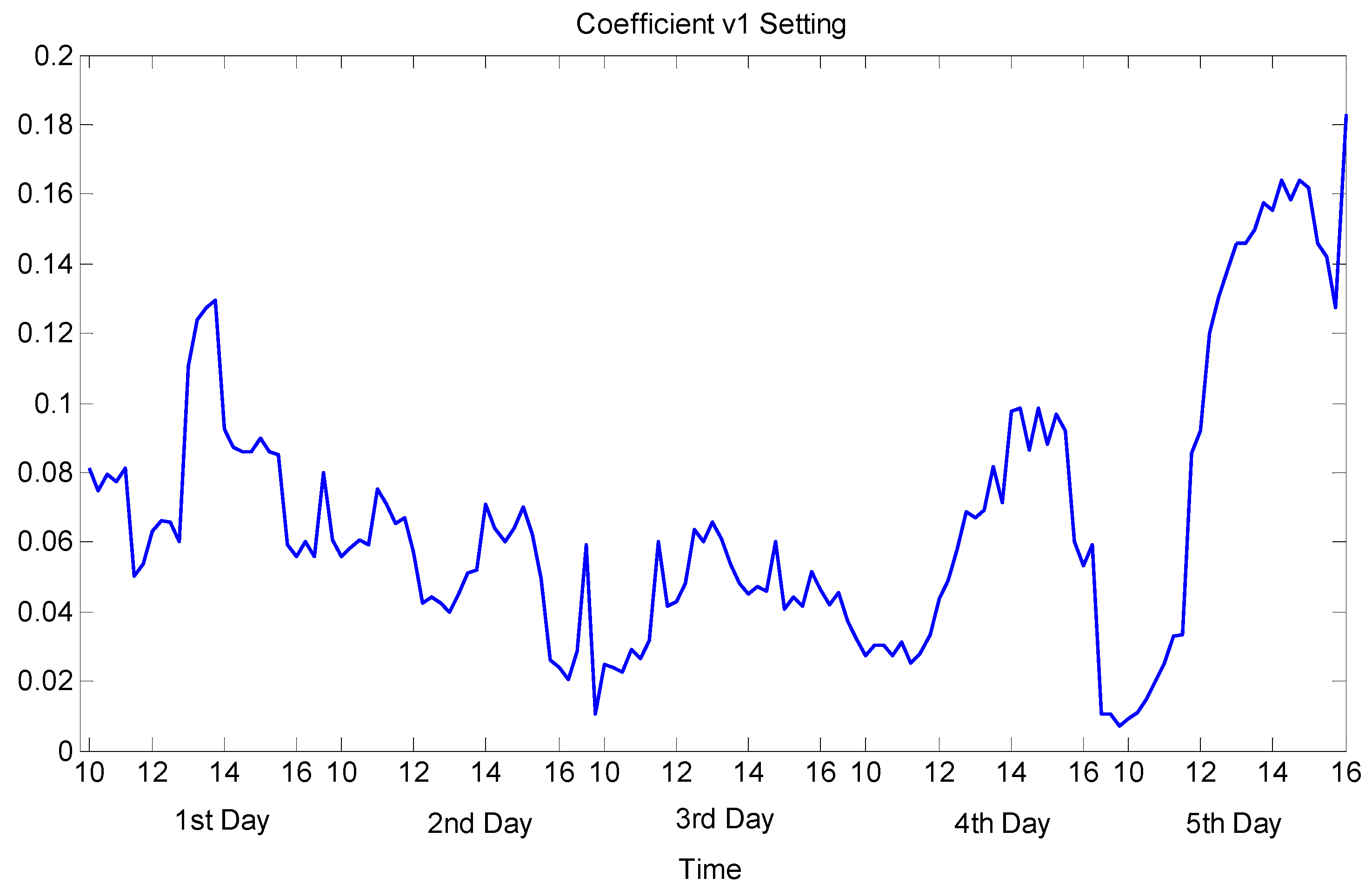
Figure 5.
The variation of coefficient v2.

Figure 6.
Comparison between the optimized load shed Ψ(kTs), the target load shedding profile P(kTs) and the upper and lower boundaries of target (1 − ν1)P(kTs) and (1 + ν2)P(kTs).
Figure 6.
Comparison between the optimized load shed Ψ(kTs), the target load shedding profile P(kTs) and the upper and lower boundaries of target (1 − ν1)P(kTs) and (1 + ν2)P(kTs).
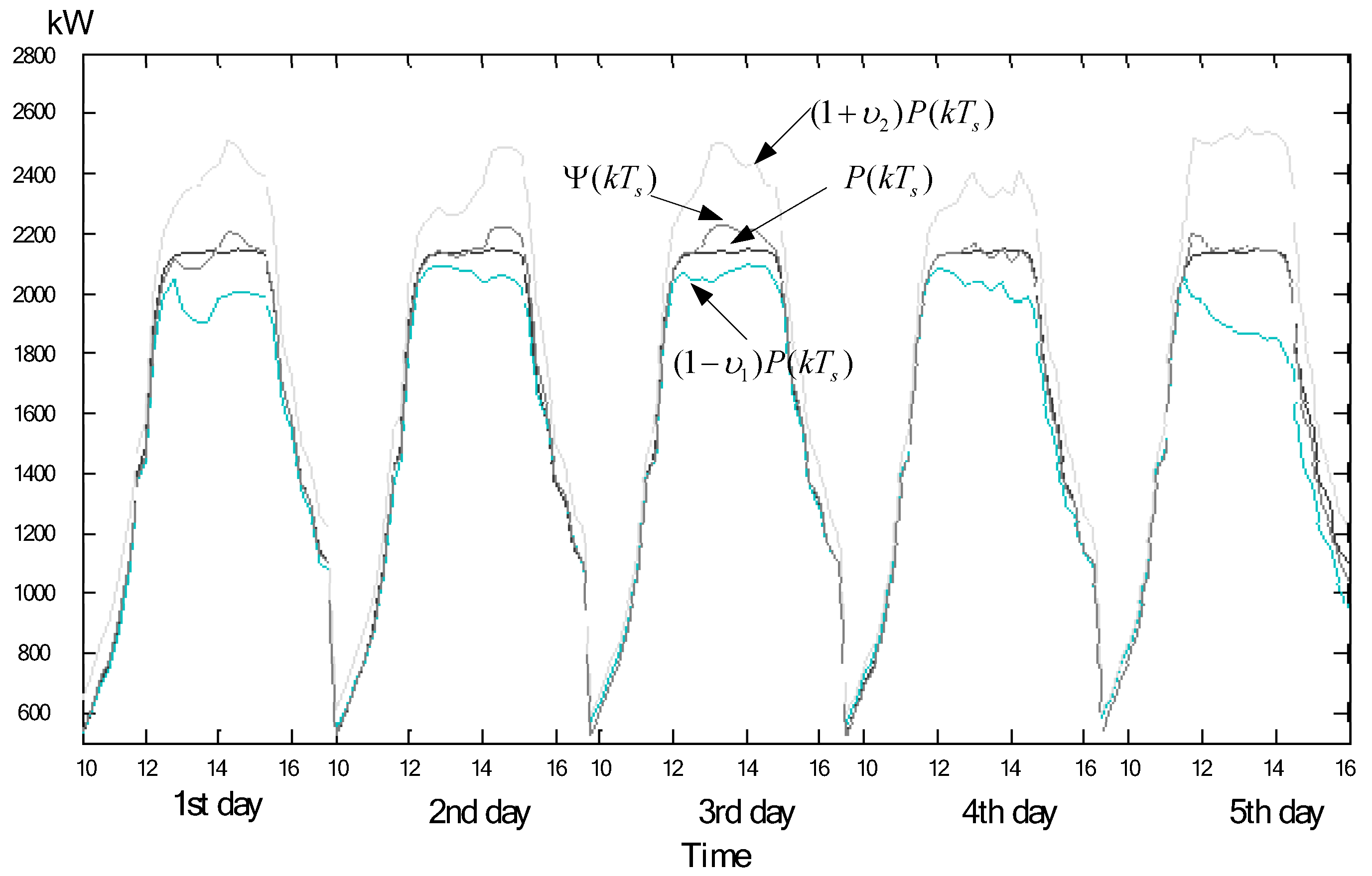
Figure 7.
(a) Variation of optimized load shedding contribution ratios obtained by customer with the largest capacity. (b) Variation of controllable load profile for customer with the largest capacity.
Figure 7.
(a) Variation of optimized load shedding contribution ratios obtained by customer with the largest capacity. (b) Variation of controllable load profile for customer with the largest capacity.

Figure 8.
Changes of standard deviation of shedding contribution ratios (a) with (b) without considering the filtering scheme in defined (20).
Figure 8.
Changes of standard deviation of shedding contribution ratios (a) with (b) without considering the filtering scheme in defined (20).

Table 1.
Simulation parameters including the actual capacity, maximum controllable load and the time constraints to remain in under-controlled and off-controlled status for each customer.
Table 1.
Simulation parameters including the actual capacity, maximum controllable load and the time constraints to remain in under-controlled and off-controlled status for each customer.
| i | Capacity (kW) | Max () (kW) | (min) | (min) |
|---|---|---|---|---|
| 1 | 250 | 109 | 15 | 30 |
| 2 | 350 | 219 | 30 | 15 |
| 3 | 750 | 296 | 30 | 15 |
| 4 | 800 | 466 | 30 | 15 |
| 5 | 1000 | 585 | 30 | 15 |
| 6 | 1150 | 727 | 30 | 15 |
| 7 | 1350 | 772 | 30 | 15 |
| 8 | 1430 | 930 | 30 | 15 |
| 9 | 1800 | 1093 | 30 | 30 |
| 10 | 2100 | 1194 | 30 | 15 |
| 11 | 250 | 140 | 30 | 15 |
| 12 | 500 | 237 | 15 | 30 |
| 13 | 800 | 347 | 15 | 30 |
| 14 | 800 | 494 | 30 | 30 |
| 15 | 1100 | 698 | 30 | 15 |
| 16 | 1300 | 727 | 15 | 16 |
| 17 | 1380 | 846 | 30 | 17 |
| 18 | 1550 | 1018 | 30 | 18 |
| 19 | 2000 | 1083 | 15 | 19 |
| 20 | 2400 | 1198 | 30 | 20 |
| 21 | 320 | 193 | 15 | 21 |
| 22 | 530 | 253 | 30 | 22 |
| 23 | 800 | 461 | 30 | 23 |
| 24 | 930 | 510 | 30 | 24 |
| 25 | 1100 | 669 | 30 | 25 |
| 26 | 1320 | 740 | 30 | 26 |
| 27 | 1400 | 905 | 30 | 27 |
| 28 | 1720 | 1045 | 30 | 28 |
| 29 | 2100 | 1131 | 30 | 29 |
| 30 | 2400 | 1427 | 30 | 30 |
© 2018 by the authors. Licensee MDPI, Basel, Switzerland. This article is an open access article distributed under the terms and conditions of the Creative Commons Attribution (CC BY) license (http://creativecommons.org/licenses/by/4.0/).
Share and Cite
MDPI and ACS Style
Yao, L.; Yao, L.; Lim, W.H. A Soft Curtailment of Wide-Area Central Air Conditioning Load. Energies 2018, 11, 492. https://doi.org/10.3390/en11030492
AMA Style
Yao L, Yao L, Lim WH. A Soft Curtailment of Wide-Area Central Air Conditioning Load. Energies. 2018; 11(3):492. https://doi.org/10.3390/en11030492
Chicago/Turabian StyleYao, Leehter, Lei Yao, and Wei Hong Lim. 2018. "A Soft Curtailment of Wide-Area Central Air Conditioning Load" Energies 11, no. 3: 492. https://doi.org/10.3390/en11030492
Note that from the first issue of 2016, this journal uses article numbers instead of page numbers. See further details here.