Time Traveling Regularization for Inverse Heat Transfer Problems
by
 ,
,
Elisan Dos Santos Magalhães
 ,
,
Bruno De Campos Salles Anselmo
,
Ana Lúcia Fernandes de Lima e Silva
and
Sandro Metrevelle Marcondes Lima e Silva
* Heat Transfer Laboratory—LabTC, Institute of Mechanical Engineering—IEM, Federal University of Itajubá—UNIFEI, Campus Prof. José Rodrigues Seabra, Av. BPS, 1303, 37500-903 Itajubá, MG, Brazil
*
Author to whom correspondence should be addressed.
Energies 2018, 11(3), 507; https://doi.org/10.3390/en11030507
Submission received: 4 January 2018
/
Revised: 16 February 2018
/
Accepted: 19 February 2018
/
Published: 27 February 2018
(This article belongs to the Section I: Energy Fundamentals and Conversion)
Abstract
:This work presents a technique called Time Traveling Regularization (TTR) applied to an optimization technique in order to solve ill-posed problems. This new methodology does not interfere in the minimization technique process. The Golden Section method together with TTR are applied only to the objective function which will be minimized. It consists of finding an ideal timeline that minimizes an objective function in a defined future time step. In order to apply the proposed methodology, inverse heat conduction problems were studied. Controlled experiments were performed on 5052 aluminum and AISI 304 stainless steel samples to validate the proposed technique. One-dimensional and three-dimensional heat input experiments were carried out for the 5052 aluminum and AISI 304 stainless steel samples, respectively. The Sequential Function Specification Method (SFSM) was also used to be compared with the results of heat flux obtained by TTR. The estimated heat flux presented a good agreement when compared with experimental values and those estimated by SFSM. Moreover, TTR presented lower residuals than the SFSM.
1. Introduction
In mathematical physics, solving a direct problem usually means finding a mathematical function that describes a phenomenon or a process of a given domain at any time instant. However, many transient and non-linear problems do not have a direct solution for their governing equations. In those cases, the development of new approaches and techniques to solve those problems is necessary. Among these, there are the techniques based on the solution of inverse problems. The inverse model aims to find a cause from an effect or observation. This particular situation is often called ill-posed problems [1].
A stability criterion that could be used to minimize the divergence on the solutions is the regularization method proposed by Tikhonov and Arsenin [2]. This method is usually applied together with an inverse or optimization method. Likewise, there is a relatively many procedures that have been studied in the last years for the solution of ill-posed problems. For example, Grasmair et al. [3] developed a stability and convergence theory to regularize ill-posed problems for the residual method. Solodky and Volynets [4] proposed a new algorithm to solve a linear ill-posed problem with operators of finite smoothness. The algorithm used a semi-iterative method for the regularization of the original problem in combination with an adaptive strategy of discretization. Zhan and Mammadov [5] considered a method based on the Karush-Kuhn-Tucker condition, Fisher-Burmeister function and the discrepancy principle for solving linear ill-posed problems. Cheng et al. [6] studied the problem by analyzing the regularization and the conditional stability. A statistical approach is also used for the solution of inverse problems [7].
In mechanical engineering, heat transfer studies usually use inverse methods to solve ill-posed problems. As a matter of fact, some inverse techniques have been developed in order to solve heat transfer problems, for instance, the acclaimed Sequential Function Specification Method (SFSM) developed by Beck et al. [8] to minimize the heat input on a plate. However, this technique is based on Duhamel’s theorem which is only valid for linear problems [8]. Despite its limitations, Duhamel’s theorem is often used to determine the heat input in several processes [9,10]. Therefore, it should not be applied to phase change problems. This technique is currently being used to estimate heat input in many applications, for example [11,12,13]. Another inverse methodology used to estimate the heat input is the Bayesian approach, which models the entire problems in terms of probability in order to obtain the unknown variable [14,15]. Zhou et al. [16] proposed a modified Duhamel’s theorem method for the surface heat flux estimation of transient ultra-fast surface cooling. In this work, the authors compared the surface heat flux estimation of the proposed method with Duhamel’s theorem, SFSM, and the Transfer Function method. There is also the use of filter solutions that allow the heat flux estimation, for instance [17]. Some authors use the Trefftz approach to minimize the heat transfer on steady problems [18], while others present general methods to solve inverse heat transfer problems [19,20].
Another option to minimize variables is the optimization technique. For example, Magalhães et al. [21] applied the Broyden-Fletcher-Goldfarb-Shano (BFGS) method to estimate the thermal efficiency in Aluminum Gas Tungsten Arc Welding (GTAW) process; Hosseni et al. [22] applied the Conjugate Gradient method to estimate the heat input in a friction stir welding. However, the major problem of those techniques is the susceptibility to the interference of noise on the estimated parameter in the experiments. Therefore, those techniques use only the average data estimated in the heated region. When this factor is considered, the estimated parameter converges to the expected value.
This work aims to present a technique which can be applied with the optimization techniques in order to have a better approach of the estimated curves on transient problems. The method is based on the Time-Traveling concept and it is applied to the objective function. The Golden Section technique [23] is used in order to estimate the imposed heat flux on sample surfaces. This technique was chosen due to its non-linear characteristic. The TTR can be applied to any optimization technique that requires an objective function. The proposed method is compared with the SFSM [7] in order to present its reliability.
2. Methodology
Heat Transfer Model
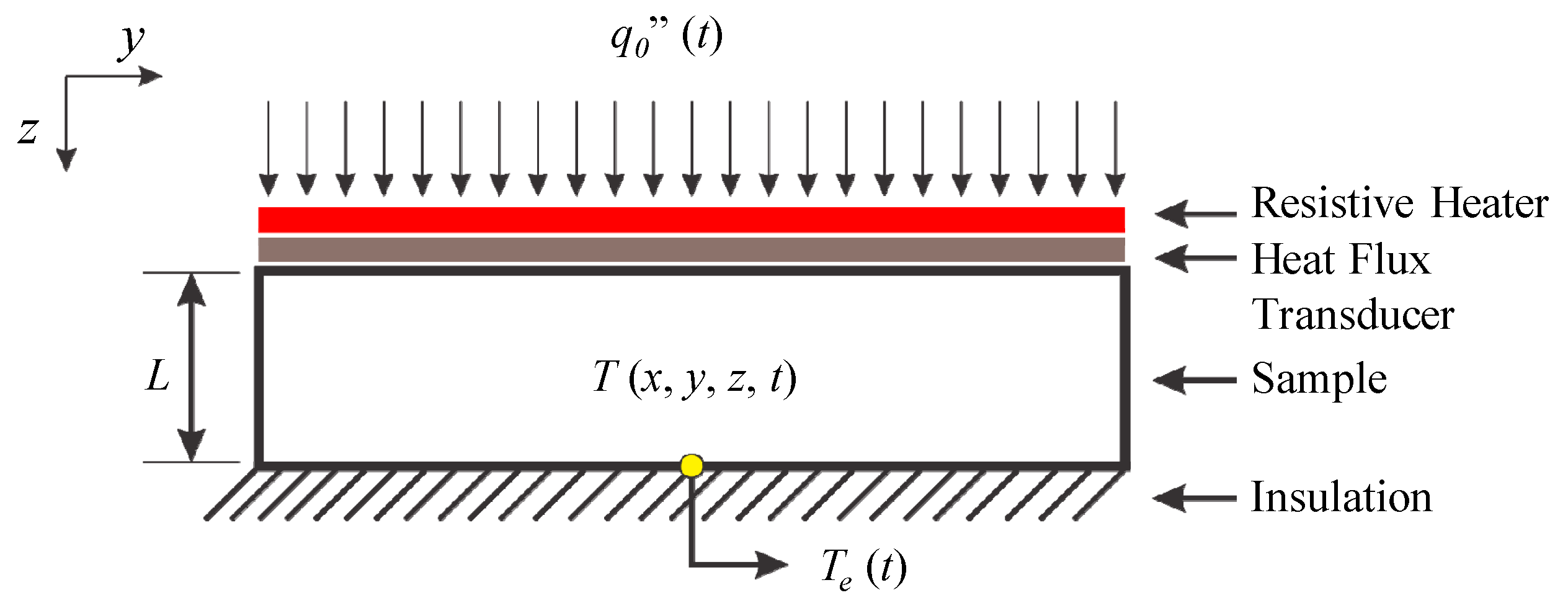
In this work, a three-dimensional heat transfer model was studied. The thermal model is approximated by using the finite difference method with the implicit formulation. The thermal properties are considered constant in the temperature interval analyzed. The transient 3D conduction equation for the problem presented in Figure 1 could be written as:
where x, y, and z are the Cartesian Coordinates, L, H and W are the dimensions of the sample in directions x, y and z respectively, t is the physical time, tf is the experimental or simulated total time, and α is the thermal diffusivity.
Equation (1) is subjected to the boundary condition of a uniform imposed heat flux on surface A, while the other surfaces are subjected to the boundary condition of insulation. The boundary and initial conditions are given by:
where λ is the thermal conductivity, q” is the estimated heat flux, and T∞ is the room temperature. A C++ code was built in order to solve the linear system of the equations obtained through the application of the finite difference method. These equations are solved through the Modified Strongly Implicit procedure method [24].
3. The Inverse Heat Conduction Problem (IHCP)
The proposed methodology is applied to an Inverse Heat Conduction Problem (IHCP). As presented by Beck and Woodbury [13], the measured temperature vector Y with n elements can be represented by:
The calculated temperature vector T can be represented by:
Both elements represent temperature points collected in the same location. The unknown heat flux is represented by:
Calculated temperature vector, T, can be obtained by the Finite Difference method through the solution of the following linear system:
where A represents the finite difference coefficient matrix and B the finite difference source term.
A T = B
3.1. Time Traveling Regularization (TTR)
The proposed technique consists of an initial guess which analyses a hypothetical timeline. Then, it compares the parameter which will be minimized in a future time. If the guess does not suit the optimum condition in a future time, the method returns to the present time and changes the guess. In other words, the method analyzes how the effect of a simple guess will affect the response in a future time.
In many kinds of experimental measurements, there is a settling time between the physical or thermal excitation and the measurements. This methodology allows minimizing this settling time in order to maximize the estimation. Consequently, this configuration reduces the number of required future time steps which can overcome the settling time of the sample.
Algorithm 1 presents the implementation of the TTR with the Golden Section method for an inverse heat transfer problem. In this algorithm, the heat flux is estimated by minimizing an objective function defined by the square difference between the experimental and numerical temperatures. In Algorithm 1, enter the input variables as the thermal properties, initial conditions, experimental temperatures, stop criterion ε and a variable r which represents the number of future time steps. Counter i represents the number of interactions which the model uses to simulate a case. In general, reference imax (Algorithm 1 line 6) is defined by the number of collected temperature points subtracting r. Temperature matrix T for counter i is stored in T* to save the previous value. This value is required in the optimization process. The Golden Section minimization method is started in line 8. Values qmin and qmax are the limits for the estimated heat flux. Xl, Xu, X1, and X2 are Golden Section variables that allow the heat flux estimation, while F1 and F2 store the objective function value. The Golden Section ratio variable τ has the value of [23].
| Algorithm 1: The Golden Section Algorithm with Time Travelling Regularization | ||
| 1: | Start | |
| 2: | Given the input variables | |
| 3: | Define the tolerance for the objective function ε | |
| 4: | T = Define the initial condition | |
| 5: | Define the number of future times r | |
| 6: | for i = 1; i ≥ imax; i = i + 1 | |
| 7: | T* = T | |
| 8: | Xl = qmin | |
| 9: | Xu = qmax | |
| 10: | X1 = (1 − τ) Xl + τ Xu | |
| 11: | qi = X1 | |
| 12: | F1 = 0 | |
| 13: | for j = i; j ≤ i + r; j = j + 1 | TTR |
| 14: | A = Evaluate the coefficients for the step j | |
| 15: | B = Evaluate the source term for the step j | |
| 16: | T = A−1 B (Solve the direct model) | |
| 17: | F1 = F1 + (Yj − Tj)2 | |
| 18: | end for | |
| 19: | T = T* | |
| 20: | X2 = τ Xl + (1 − τ) Xu | |
| 21: | qi = X2 | |
| 22: | F2 = 0 | |
| 23: | for j = i; j ≤ i+r; j = j + 1 | TTR |
| 24: | A = Evaluate the coefficients for the step j | |
| 25: | B = Evaluate the source term for the step j | |
| 26: | T = A−1 B (Solve the direct model) | |
| 27: | F2 = F2 + (Yj − Tj)2 | |
| 28: | end for | |
| 29: | do | |
| 30: | T = T* | |
| 31: | if F1 > F2 | |
| 32: | Xl = X1 | |
| 33: | Fl = F1 | |
| 34: | X1 = X2 | |
| 35: | F1 = F2 | |
| 36: | Re-evaluate lines 20-28 | |
| 37: | Fobj = F1 | |
| 38: | Endif | |
| 39: | Else | |
| 40: | Xu = X2 | |
| 41: | Fu = F2 | |
| 42: | X2 = X1 | |
| 43: | F2 = F1 | |
| 44: | Re-evaluate lines 10-18 | |
| 45: | Fobj = F2 | |
| 46: | endif | |
| 47: | while (Fobj > ε) | |
| 48: | T = T* | |
| 49: | A = Evaluate the coefficients for the step i | |
| 50: | B = Evaluate the source term for the step i | |
| 51: | T = A−1B (Solve the direct model for qopt) | |
| 52: | end for | |
| 53: | End | |
The optimization method starts by defining the guess values for the minimization process (lines 10 and 11). The objective function (F1) is defined as 0. The heat flux variable q is used to store the guess values (lines 11 and 21). The TTR methodology is then applied between lines 13 to 18 and lines 23 to 28. Given the heat flux as a constant value, counter j replaces counter i and an iterative process starts considering a constant heat flux in the time interval comprised between the time represented by counter i and the time represented by i + r (lines 13 and 23). In those loops, coefficient matrix A and the source term B are evaluated. The numerical temperature is then calculated by solving the linear system represented by lines 16, 26 and 51. The objective functions F1 and F2 are then evaluated in a sum (Equation (10)) for counter j. The temperature is then restarted to the previous value (lines 19, 30 and 48). The Golden Section method loop starts in line 29 and is then evaluated until the objective function Fobj is lower than the tolerance ε (line 22). After the loop, the optimal value for the heat flux qi is then estimated. The temperature should be updated with estimated qi. However, it should be calculated for only the time represented by counter i. Thus, this algorithm analyzes how the temperature behaves if the heat flux is temporarily held constant for r future time steps.
3.2. The TTR Objective Function
The TTR does not interfere with the minimization procedure. However, it modifies the objective function in order to have the temporal analysis. Thus, the Objective Function is minimized in a future time step rather than in the present time step. For example, Equation (7) presents a usual objective function adjusted to the TTR:
where Fobj is the objective function, j is the index of time, r is the number of future time steps, and are the experimental and numerical temperatures respectively at time index j + r. In this equation, the introduction of r reduces the noise on the estimated parameter significantly. As r increases, this numerical noise decreases. However, in order to achieve the predetermined r, the temperature at time index r − 1, r − 2, …, 1 and 0 should be evaluated. Thus, the objective function may also consider these terms as follows:
3.3. Settling Time
The use of TTR requires that the number of future time steps multiplied by the time interval should be twice or three times higher than the settling time, which is usually measured experimentally. The Settling Time could be obtained as presented by Shirtliffe [25] for a constant heat flux as:
where St is the Settling Time, Lc is the characteristic length, α is the thermal diffusivity, and em is measurement error.
3.4. Sequential Function Specification Method (SFSM)
As in TTR, the Sequential Function Specification Method (SFSM) also temporarily considers the heat flux as constant for r future time steps [8]. The main difference is how the numerical temperatures are obtained. The algebraic equation for the SFSM at time tM is:
where ϕi is the dimensionless temperature for a unit surface heat flux, S is the sensitivity matrix, which is a square matrix of n elements given by:
The numerical values of the first column of Equation (12) are approached by setting the temperature to zero and the heat flux to unit value [13].
3.5. Tikhonov Regularization
In this work, the Tikhonov regularization [2] was used in order to compare the results. A first order regularization was applied using the Golden Section method. The main goal was to minimize the following objective function:
where γ represents the regularization parameter and qref is the heat flux reference value. The regularization parameter γ was defined according to the L-curve [26].
4. Experimental and Numerical Procedure
4.1. One-Dimensional Experiment Using Aluminum 5052
In order to present the versatility of the methodology, two experimental conditions were tested at the Heat Transfer Laboratory (LabTC) of the Federal University of Itajubá. The experiments have only the feature of proving the feasibility of the methodology. Therefore, only three experiments of each case were conducted in order to assure the repeatability.
In the first one, a one-dimensional experiment was conducted in Aluminum 5052 samples. Figure 2 presents the experimental thermal model, where a homogeneous 50 × 50 × 6.2 mm3 Aluminum 5052 sample was positioned as presented. The sample was uniformly heated with an intensity of q0”(t), with a 50 × 50 × 0.2 mm3 Kapton resistive heater. This imposed heat flux was measured through a heat flux transducer. All the other surfaces were insulated with expanded polystyrene. The temperature signals were measured in the center of the opposite heated surface. A HP 75000 Series B data acquisition system, together with a computer was used in order to collect the temperature signals. 2024 temperature points were collected for a time step of 0.396 s. This time step was automatically defined by the data acquisition system.
In order to minimize the heat flux, the C++ code took into account the values of the thermal conductivity λ = 137 W/m.K. and thermal diffusivity α = 5.59 × 10⁻⁵ m2/s for Aluminum 5052 [27]. The software considered the boundary condition of applied heat flux on the top surface and the insulated condition on all other surfaces. A convergence mesh test was performed in order to verify the ideal mesh. A refined mesh with 300,000 volumes was applied.
4.2. Three-Dimensional Experiment Using AISI 304
In the second experiment, a three-dimensional experimental condition was achieved on two symmetrically assembled 60 × 100 × 9.5 mm3 AISI 304 stainless steel plate. A Kapton heater, similar to the one used with Aluminum 5052, was used. Each experiment lasted 250 s. In the first 30 s, the DC power supply was turned off. Then it was switched on for 70 [s] imposing a heat flux of about 3800 W/m². Finally, in the last 150 s, the power supply was turned off. The data acquisition system read temperature at a time interval of 0.2 s totalizing 1250 temperature points. The thermal diffusivity α = 3.77 × 10⁻⁶ m2/s and thermal conductivity λ = 14.7 W/m.K of AISI 304 were obtained from Carollo et al. [28]. The adopted values for heat flux and heating time were chosen in order to ensure a temperature difference lower than 7 °C. Therefore, the thermal properties may be considered constant in this temperature interval. Figure 3a presents the experimental assembly of the sample and heater and Figure 3b presents the symmetrical assembly of the experiment as well as the position of the thermocouple. The expanded polystyrene was used for the insulation of the experiment. As the resistive heater did not cover all the upper surface of the sample, the heat flux distribution was not uniform.
5. Random Error Analysis
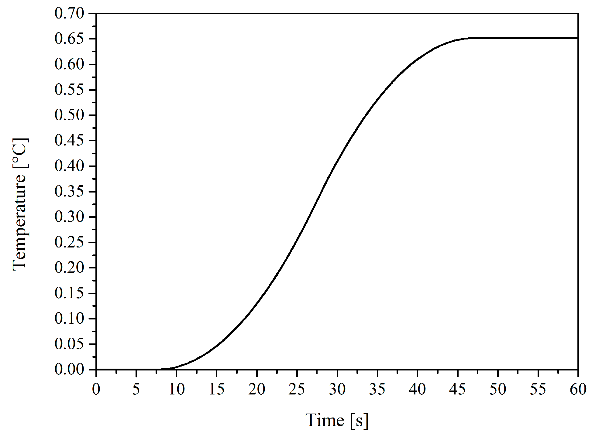
In order to compare the TTR with the SFSM and the Tikhonov Regularization, a random error analysis is proposed [29]. This analysis considers a hypothetical experiment free from noise. Considering the one-dimensional model presented in Section 4.1, the initial condition is T(x, y, z) = 0, and a triangular hypothetical heat flux surface defined by:
The temperature response to this thermal excitation on the center of the opposite surface is presented in Figure 4.
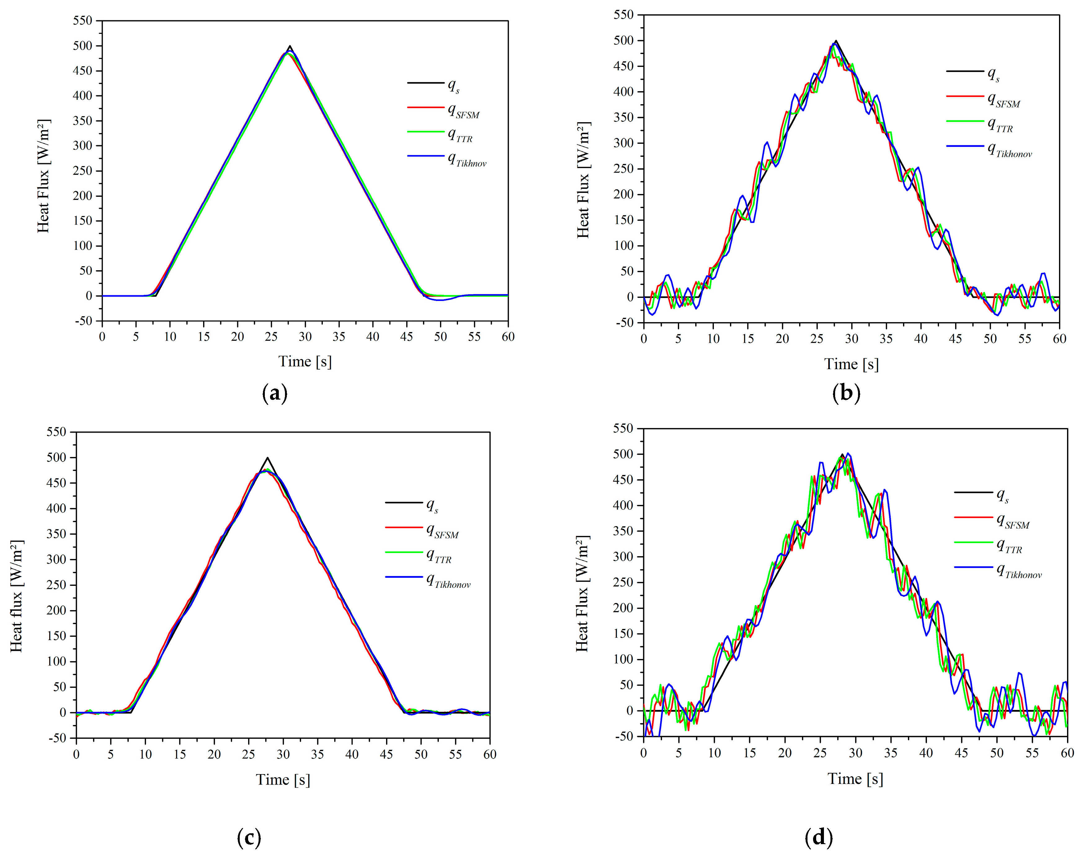
In order to evaluate the influence of noise interference on temperature data, random errors were added to the temperature response presented in Figure 4. Four conditions were analyzed where the heat input was estimated by the TTR, SFSM, and Tikhonov Regularization. In the first condition, the heat flux was estimated from the temperature response without using random errors. In the three other conditions, random errors were used in the temperature curve. The additive error vector E can be defined as:
In this case, the measured temperature vector Y is obtained from the following relation:
Y = T ± E
The additive error vector was formed by random errors in the order of 1% (±0.326 × 10⁻³ °C), 5% (±0.163 × 10⁻² °C) and 10% (±0.326 × 10⁻² °C) of the maximum temperature (0.652 °C). Figure 5 presents the estimated heat flux for the four conditions tested. From the analysis of Figure 5, it may be observed that the three estimation methods presented almost the same results. However, the SFSM and TTR presented better results than the Tikhonov Regularization when the errors in the input data increased.
6. Result Analysis
6.1. Aluminum 5052
The three experiments performed had the same configuration. Hence, the results of only one experiment are presented. Figure 6 presents the estimated heat flux for three different numbers of future time steps in TTR, r = 5, 10 and 20. It also presents the heat flux measured by the heat flux transducer on the sample. It may be noticed that as the number of future time steps increases, the noise in the heated region (60 s < t < 730 s) decreases slightly. Therefore, as presented in Figure 6, the estimated curve with r = 20 has a lower noise signal than r = 10 or 5. However, this noise reduction is too small. This could be explained as TTR bypasses the settling time of the material. The settling time depends on the characteristic length, measurement error, and the thermal diffusivity. The estimated settling time for the Aluminum 5052 sample was about 1 s. The time interval in the numerical analysis was 0.396 s. Therefore, it took at least three future time steps to bypass the settling time and achieve good results.
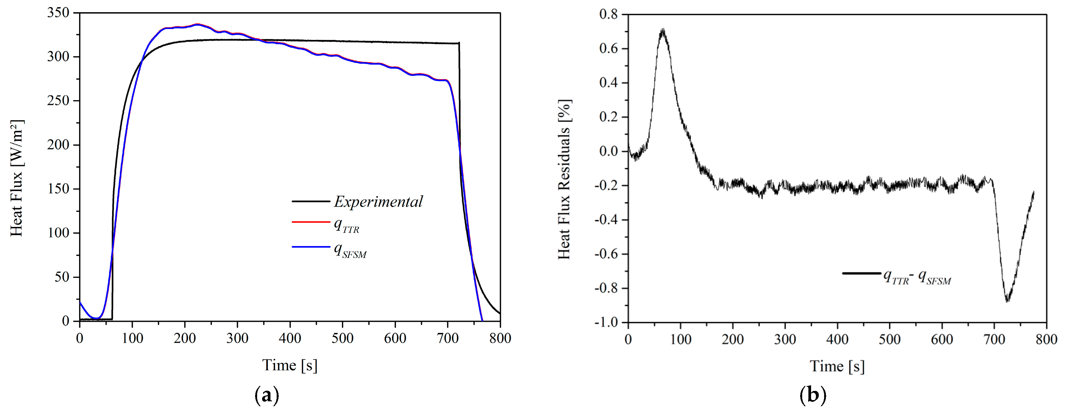
In the heated region, the estimated heat flux presented average differences of approximately 5% compared to the experimental measurements. This difference may be explained: the first factor is the errors of the heat flux transducer measurements and the second factor is the uncertainties of the thermocouple measurements in aluminum. A third factor is a small oscillation on current or voltage that will interfere significantly with the temperature measurement. Since the estimation process takes into account only the measured temperatures, the estimated heat flux curve will be affected. In order to confirm the good results of TTR, SFSM [8] was used to estimate the heat flux. The Specification Function also takes r into account. For both methods, r = 60 was chosen. Figure 7 presents a comparison of the estimated heat flux through the SFSM, TTR and the experimental measurement. It could be noticed that in Figure 7a, TTR has almost the same behavior as SFSM. However, by analyzing Figure 7b, the estimated heat flux through SFSM is lower than through TTR. This can be related to the linear characteristic of SFSM. A final factor explains what happens at the end of the experiment. When the heater is turned off SFSM does not follow the experimental curve. Thus, it indicates that the heat flux keeps being imposed on the sample (750 < t < 780 s). On the other hand, TTR is closer to the experimental curve when the heat source is turned off. This may indicate that the methodology is more accurate to deal with abrupt changes on the estimated variable than SFSM. This is associated with the objective function used in this work. The regression model only has the role of regularizing the objective function.
Another validation could be obtained by comparing the experimental and calculated temperatures. Thus, the numerical temperatures were calculated using the estimated heat flux through TTR and SFSM (Figure 8). In both cases, good results were obtained.
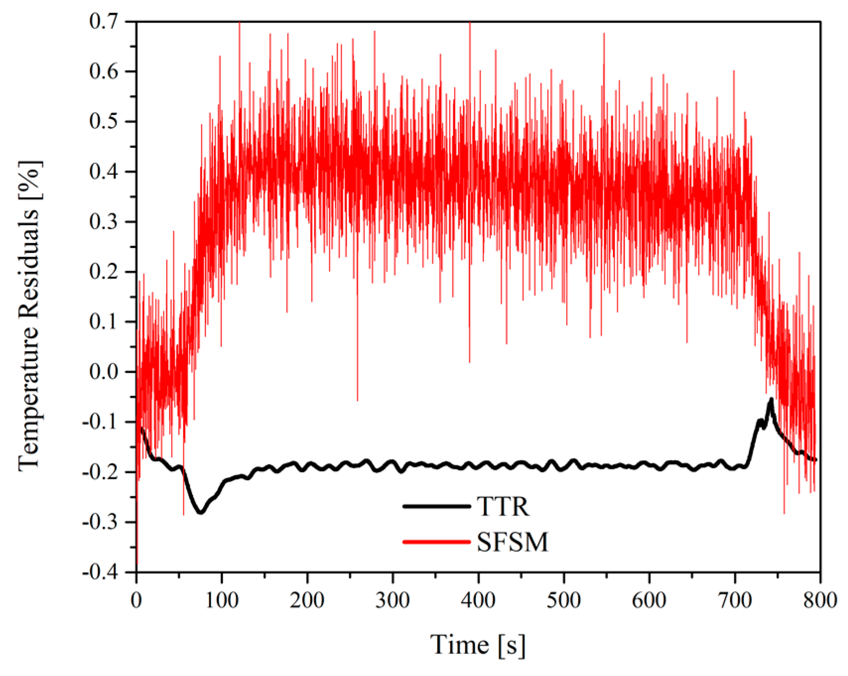
In order to analyze the precision of the estimation, Figure 9 presents the temperature residuals for TTR and SFSM. The temperature residuals are obtained through the difference between the measured and calculated temperatures divided by the maximum temperature difference. In Figure 9, the temperature residual modulus for TTR is lower than 0.04 °C and for SFSM lower than 0.10 °C. TTR presents better results and the residuals are more stable than SFSM. Indeed, the noise in the heated region for the proposed technique is almost zero and the residuals behave as a straight line. This may be associated with the optimization process that occurs when Golden Section method is used.
6.2. AISI 304 Stainless Steel
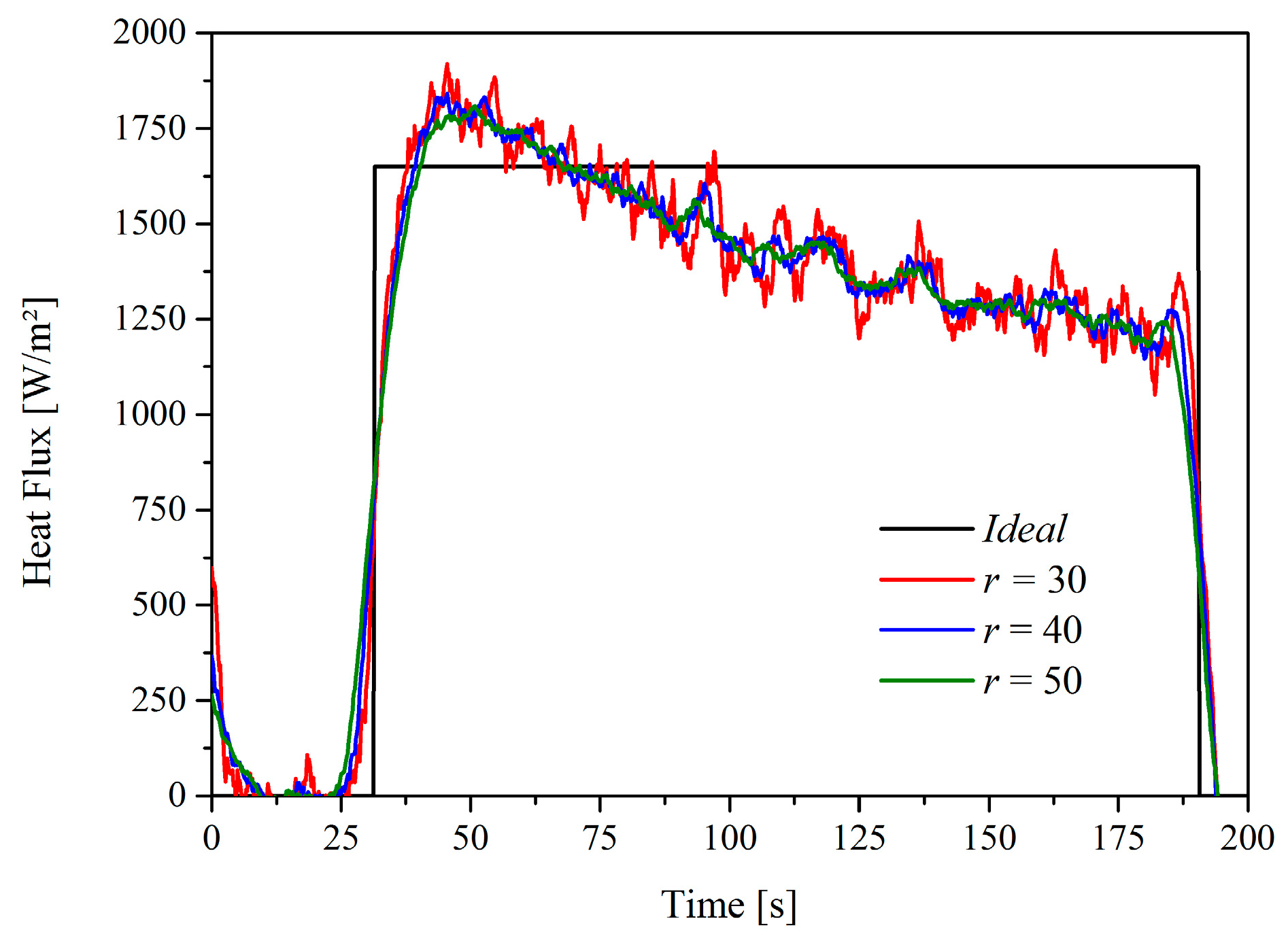
The AISI 304 stainless steel sample was thicker than the aluminum sample. In addition, the thermal conductivity of the stainless steel used is about ten times lower than that of the aluminum sample. Therefore, the estimated settling time response for the stainless-steel sample was about 2 s. In order to achieve a good result, TTR requires at least ten future time steps to minimize the result. Figure 10 presents the estimated heat flux for the experiment for three r conditions: 30, 40 and 50 and the experimental heat flux obtained from the symmetrical assembly.
It may be observed that at the beginning of the experiment the estimated heat flux overpasses the experimental one. This behavior may be related to the thermal contact resistance between the resistive heater and sample. At the beginning of the experiment, an amount of heat is stored in the thermal resistance region. Therefore, there is a delay between the beginning of the heating by the resistive heater and the effective heating on the sample. As the insulation is not perfect, there is also the heat loss by the insulation. This heat loss increases as the temperature on the sample increases affecting the estimation of the heat flux.
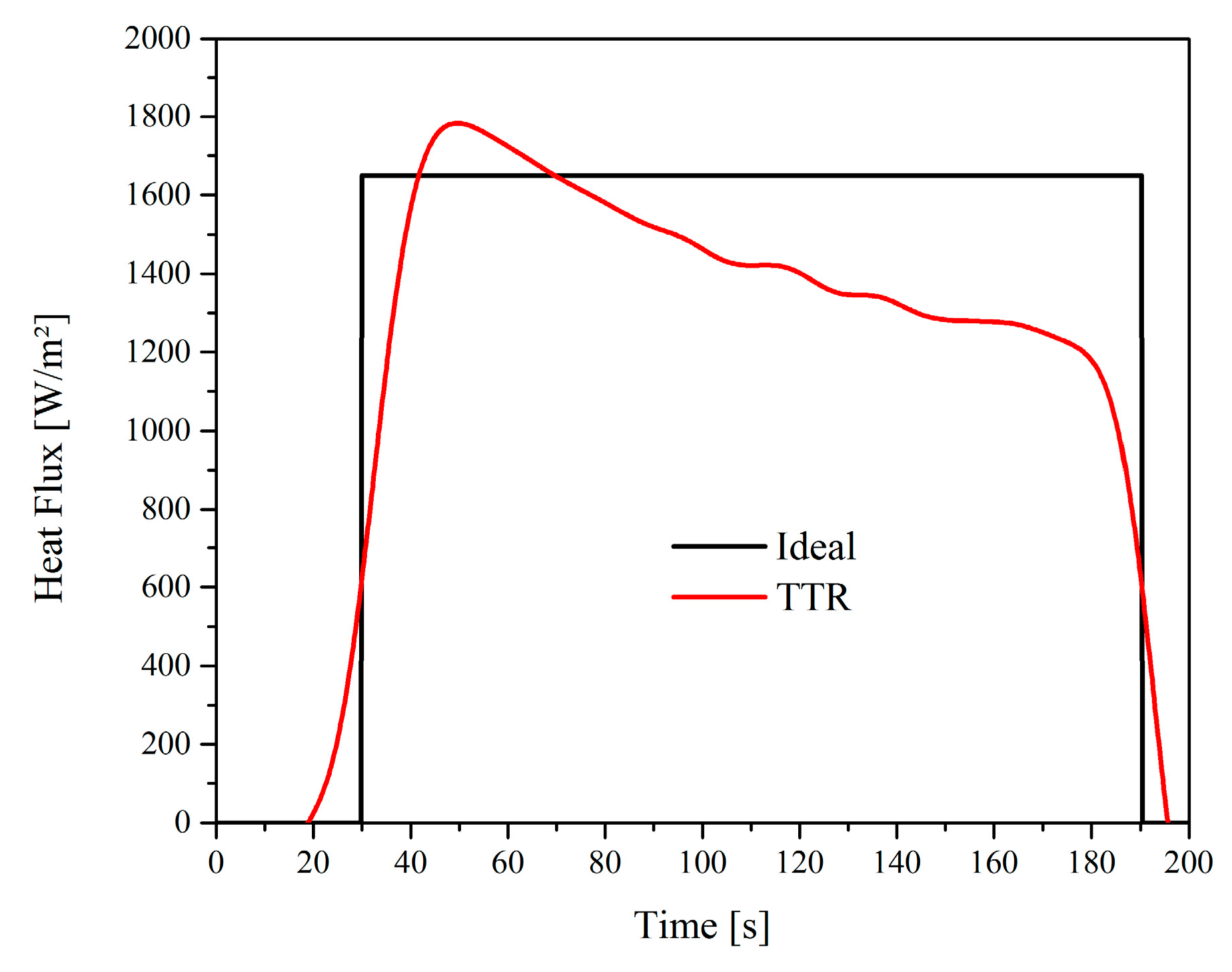
AISI 304 stainless steel presented the same behavior of the heat flux estimation as in the aluminum experiment. However, the obtained noise is relatively higher for the estimated condition with r = 30. This may be explained: As the settling time increases, more future time steps on TTR are required to overcome the settling time. There is not an ideal number of future time steps. However, the number of future time steps multiplied by the estimation time interval should be at least between two and three times the settling time of the sample. As r increases, the parameter estimation is more precise. However, the required computational time will increase substantially. For example, for r = 60, the estimated heat flux as in Figure 11 for the stainless steel almost does not present any noise in the heated region. However, it takes three times more computational time to achieve this result than for r = 20. As the presented model is three-dimensional, the required computational time to achieve the result for r = 20 is about 24 h on a computer equipped with an Intel Core i7 3.4 GHz processor. Therefore, for r = 60, the required computational time is about 72 h.
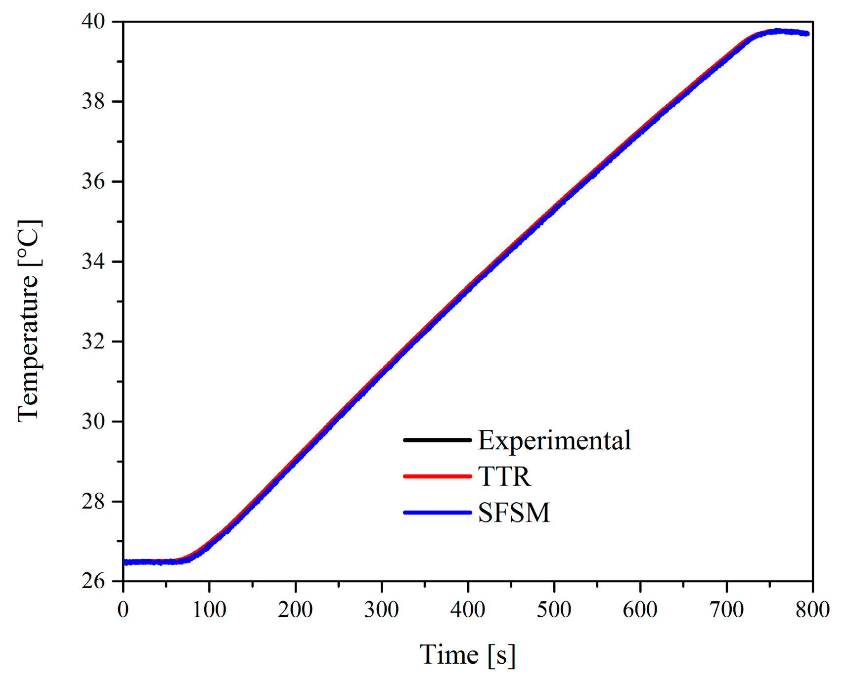
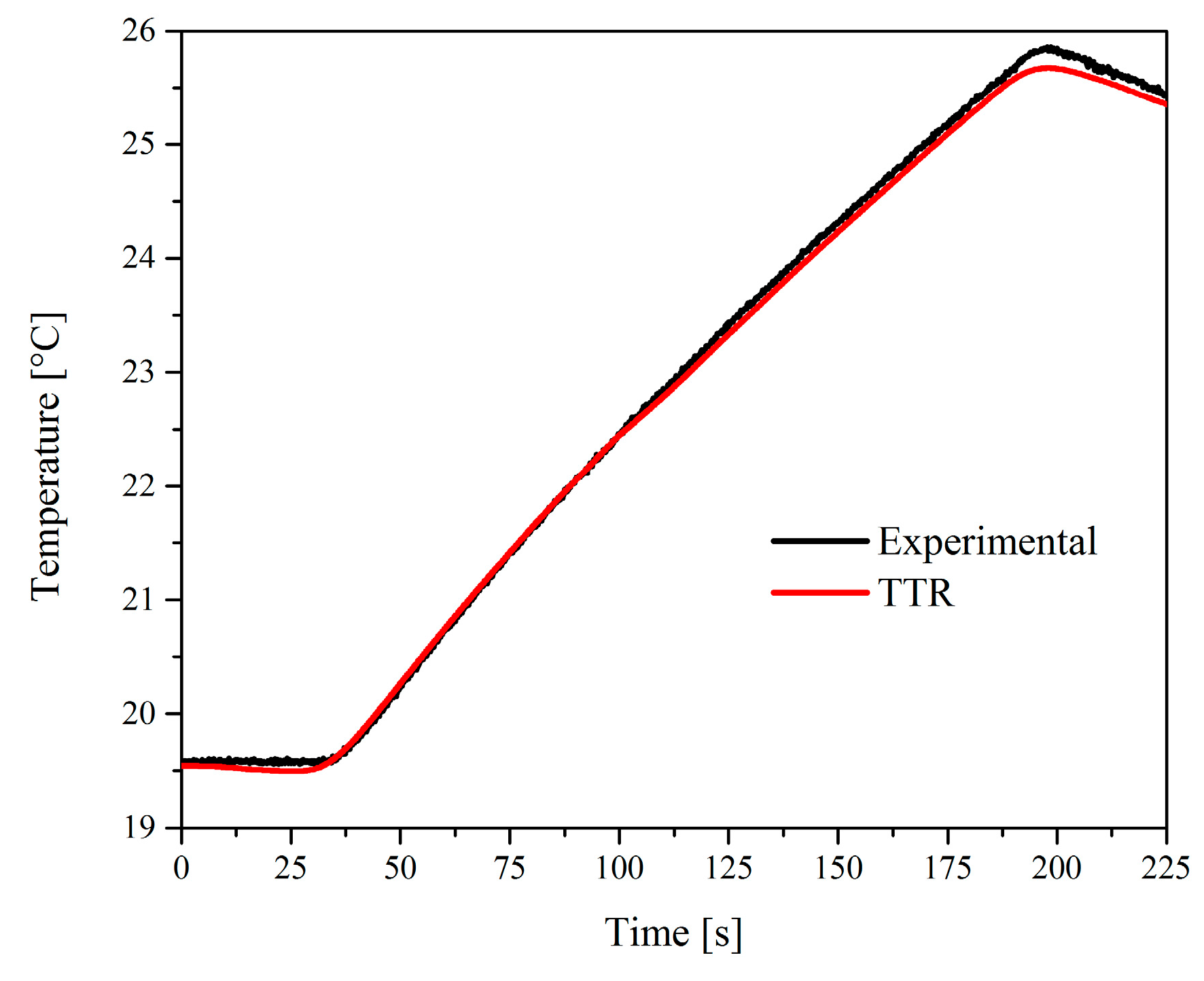
In Figure 12, a comparison between the experimental and numerical temperatures is presented. In this case, the heat flux was estimated using the Time Travelling method with r = 60. It may be noticed that the experimental and numerical temperature curves present a good agreement. For this case, the temperature residuals are lower than 0.2 °C.
7. Conclusions
This work presented a Time Traveling Regularization (TTR) technique which can be applied to some optimization techniques in order to reduce the noise in parameter estimations. In this work, the TTR was used together with the Golden Section method aiming to minimize an objective function to estimate the heat flux on ill-posed problems. The TTR proved to be an efficient way to estimate parameters that present much interference in the data. When compared with SFSM, TTR presented better results to estimate the heat flux in the region where the heating was turned off. Therefore, it can be applied to heat transfer ill-posed problems, which are worth a deep study.
Acknowledgments
The authors would like to thank CNPq, CAPES, and FAPEMIG for their financial support.
Author Contributions
Elisan dos Santos Magalhaes developed the methodology, conceived and wrote the paper; Bruno de Campos Salles Anselmo and Ana Lúcia Fernandes de Lima e Silva helped Elisan to develop the numerical code; Sandro Metrevelle Marcondes Lima e Silva to develop the manuscript and was also responsible for the experiments.
Conflicts of Interest
The authors declare no conflict of interest. The founding sponsors had no role in the design of the study; in the collection, analyses, or interpretation of data; in the writing of the manuscript, and in the decision to publish the results.
References
- Kabanikhin, S.I. Definitions and examples of inverse and ill-posed problems. J. Inverse Ill-Posed Probl. 2008, 16, 317–357. [Google Scholar] [CrossRef]
- Tikhonov, A.N.; Arsenin, V.Y. Solutions of Ill-Posed Problems. Math. Comput. 1978, 32, 1320–1322. [Google Scholar] [CrossRef]
- Grasmair, M.; Haltmeier, M.; Scherzer, O. The residual method for regularizing ill-posed problems. Appl. Math. Comput. 2011, 218, 2693–2710. [Google Scholar] [CrossRef] [PubMed]
- Solodky, S.G.; Volynets, E.A. Adaptive scheme of discretization for one semiiterative method in solving ill-posed problems. J. Mat. Sci. 2011, 175, 477–489. [Google Scholar] [CrossRef]
- Zhang, J.; Mammadov, M. A new method for solving linear ill-posed problems. Appl. Math. Comput. 2012, 218, 10180–10187. [Google Scholar] [CrossRef]
- Cheng, J.; Hofmann, B.; Lu, S. The index function and Tikhonov regularization for ill-posed problems. J. Comput. Appl. Math. 2013, 265, 110–119. [Google Scholar] [CrossRef]
- Warner, J.E.; Aquino, W.; Grigoriu, M.D. Stochastic reduced order models for inverse problems under uncertainty. Comput. Methods Appl. Mech. Eng. 2015, 285, 488–514. [Google Scholar] [CrossRef] [PubMed]
- Beck, J.; Blackwell, B.; Clair, C. Inverse Heat Conduction: Ill-Posed Problems; Wiley: New York, NY, USA, 1985; ISBN 0471083194. [Google Scholar]
- Zhou, Z.; Chen, B.; Wang, R.; Bai, F.; Wang, G. Coupling effect of hypobaric pressure and spray distance on heat transfer dynamics of R134a pulsed flashing spray cooling. Exp. Therm. Fluid Sci. 2016, 70, 96–104. [Google Scholar] [CrossRef]
- Zhou, Z.; Chen, B.; Wang, Y.; Guo, L.; Wang, G. An experimental study on pulsed spray cooling with refrigerant R-404a in laser surgery. Appl. Therm. Eng. 2012, 39, 29–36. [Google Scholar] [CrossRef]
- Somasundaram, S.; Tay, A.A.O. A study of intermittent spray cooling process through application of a sequential function specification method. Inverse Probl. Sci. Eng. 2012, 20, 553–569. [Google Scholar] [CrossRef]
- Mohammadiun, M.; Molavi, H.; Bahrami, H.R.T.; Mohammadiun, H. Application of Sequential Function Specification Method in Heat Flux Monitoring of Receding Solid Surfaces. Heat Transf. Eng. 2014, 35, 933–941. [Google Scholar] [CrossRef]
- Beck, J.V.; Woodbury, K.A. Inverse heat conduction problem: Sensitivity coefficient insights, filter coefficients, and intrinsic verification. Int. J. Heat Mass Transf. 2016, 97, 578–588. [Google Scholar] [CrossRef]
- Kaipio, J.P.; Fox, C. The Bayesian Framework For Inverse Problems In Heat Transfer. Heat Transf. Eng. 2011, 32, 83. [Google Scholar] [CrossRef]
- Franck, I.M.; Koutsourelakis, P.S. Sparse Variational Bayesian approximations for nonlinear inverse problems: Applications in nonlinear elastography. Comput. Methods Appl. Mech. Eng. 2016, 299, 215–244. [Google Scholar] [CrossRef]
- Zhou, Z.F.; Xu, T.Y.; Chen, B. Algorithms for the estimation of transient surface heat flux during ultra-fast surface cooling. Int. J. Heat Mass Transf. 2016, 100, 1–10. [Google Scholar] [CrossRef]
- Tian, J.; Chen, B.; Zhou, Z. Methodology of surface heat flux estimation for 2D multi-layer mediums. Int. J. Heat Mass Transf. 2017, 114, 675–687. [Google Scholar] [CrossRef]
- Grysa, K.; MacIag, A.; Pawinska, A. Solving nonlinear direct and inverse problems of stationary heat transfer by using Trefftz functions. Int. J. Heat Mass Transf. 2012, 55, 7336–7340. [Google Scholar] [CrossRef]
- Duda, P. A general method for solving transient multidimensional inverse heat transfer problems. Int. J. Heat Mass Transf. 2016, 93, 665–673. [Google Scholar] [CrossRef]
- Park, H.M.; Chung, O.Y. Reduction of modes for the solution of inverse natural convection problems. Comput. Methods Appl. Mech. Eng. 2000, 190, 919–940. [Google Scholar] [CrossRef]
- Magalhães, E.D.S.; de Carvalho, S.R.; de Lima E Silva, A.L.F.; Lima E Silva, S.M.M. The use of non-linear inverse problem and enthalpy method in GTAW process of aluminum. Int. Commun. Heat Mass Transf. 2015, 66, 114–121. [Google Scholar] [CrossRef]
- Hosseini, M.M.; Basirat Tabrizi, H.; Jalili, N. Thermal optimization of friction stir welding with simultaneous cooling using inverse approach. Appl. Therm. Eng. 2016, 108, 751–763. [Google Scholar] [CrossRef]
- Vanderplaats, G.N. Numerical Optimization Techniques for Engineering Design, 4th ed.; Vanderplaats Research and Development: Colorado Springs, CO, USA, 2005. [Google Scholar]
- Schneider, G.E.; Zedan, M. A Modified Strongly Implicit Procedure for the Numerical Solution of Field problems. Numer. Heat Transf. Part B Fundam. 1981, 4, 1–19. [Google Scholar] [CrossRef]
- Shirtliffe, C.J. Establishing Steady-State Thermal Conditions in Flat Slab Specimens. Heat Transm. Meas. Therm. Insul. Am. Soc. Test. Mater. 1974, ASTM STP 5, 13–33. [Google Scholar]
- Calvetti, D.; Morigi, S.; Reichel, L.; Sgallari, F. Tikhonov regularization and the L-curve for large discrete ill-posed problems. J. Comput. Appl. Math. 2000, 123, 423–446. [Google Scholar] [CrossRef]
- Lima e Silva, S.M.M.; Guimarães, G.; Silva Neto, A.J. Uma Técnica para Determinação da Capacidade de Calor Volumétrica do Alumínio 5052. Proc. Congr. Iberoam. Ing. Mech. Mérida Venezuela 2001. (In Portuguese) [Google Scholar]
- Carollo, L.F.S.; Lima e Silva, A.L.F.; Lima e Silva, S.M.M. Applying different heat flux intensities to simultaneously estimate the thermal properties of metallic materials. Meas. Sci. Technol. 2012, 23, 65601. [Google Scholar] [CrossRef]
- Woodbury, K.A. Inverse Engineering Handbook; CRC Press: Boca Raton, FL, USA, 2003. [Google Scholar]
Figure 1.
Transient 3D heat conduction problem.
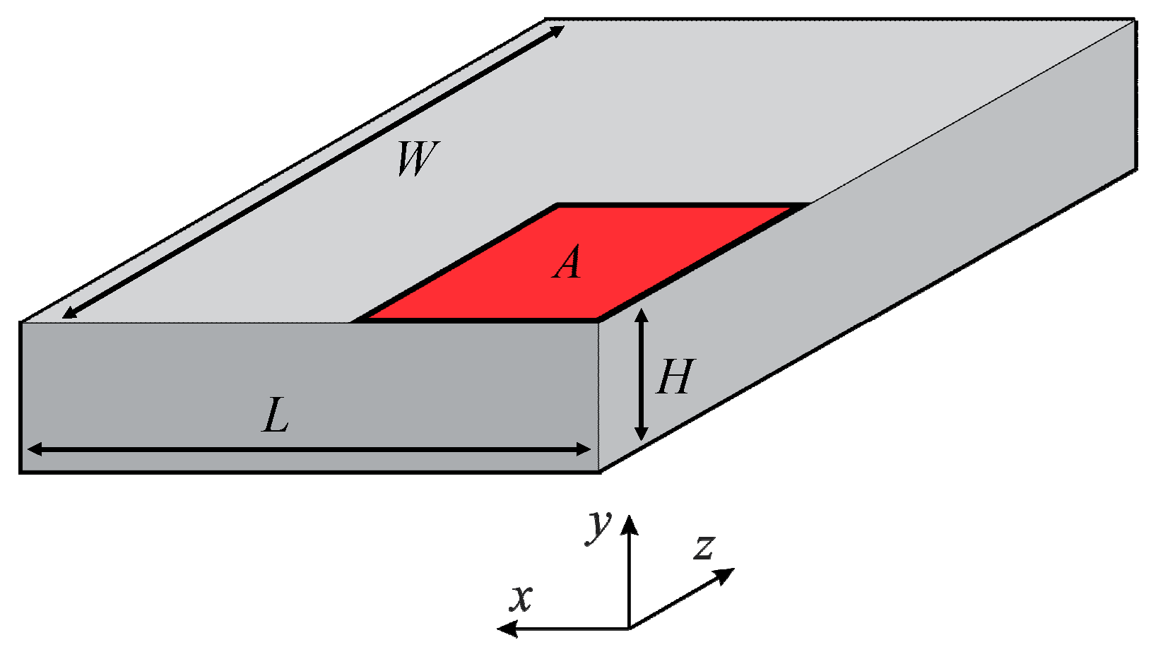
Figure 2.
One-dimensional thermal model.

Figure 3.
(a) Three-dimensional cut view of the experiment using AISI 304 stainless steel and (b) Symmetrical cut view assembly of the experiment with thermocouple.
Figure 3.
(a) Three-dimensional cut view of the experiment using AISI 304 stainless steel and (b) Symmetrical cut view assembly of the experiment with thermocouple.
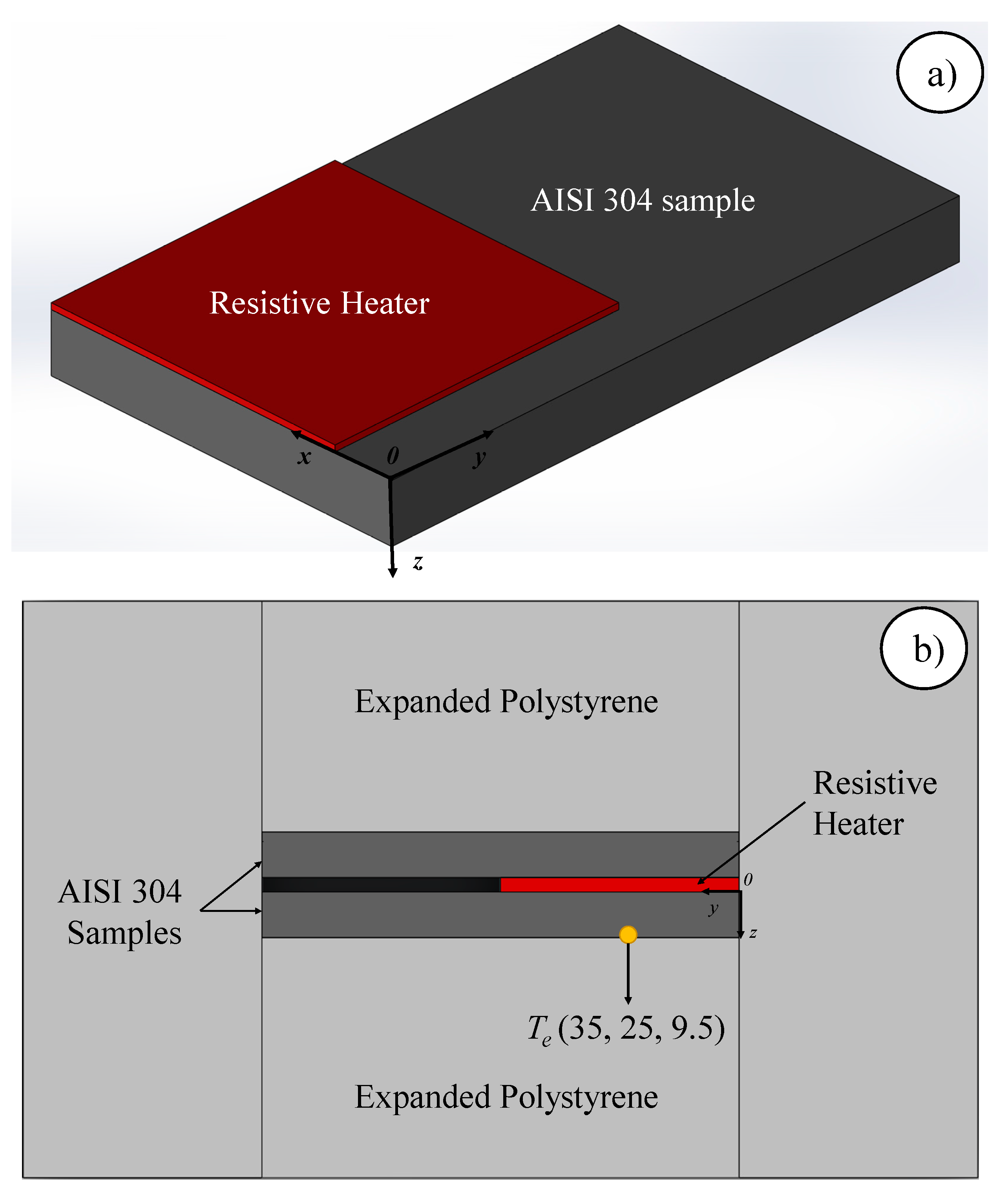
Figure 4.
Temperature response for the triangular heat flux.

Figure 5.
Estimated heat flux for the additive error vector: (a) Y = T ± 0; (b) Y = T ± 0.326 × 10⁻³; (c) Y = T ± 0.163 × 10⁻²; and (d) Y = T ± 0.326 × 10⁻².
Figure 5.
Estimated heat flux for the additive error vector: (a) Y = T ± 0; (b) Y = T ± 0.326 × 10⁻³; (c) Y = T ± 0.163 × 10⁻²; and (d) Y = T ± 0.326 × 10⁻².

Figure 6.
Comparison between the measured and estimated heat flux for Aluminum 5052.
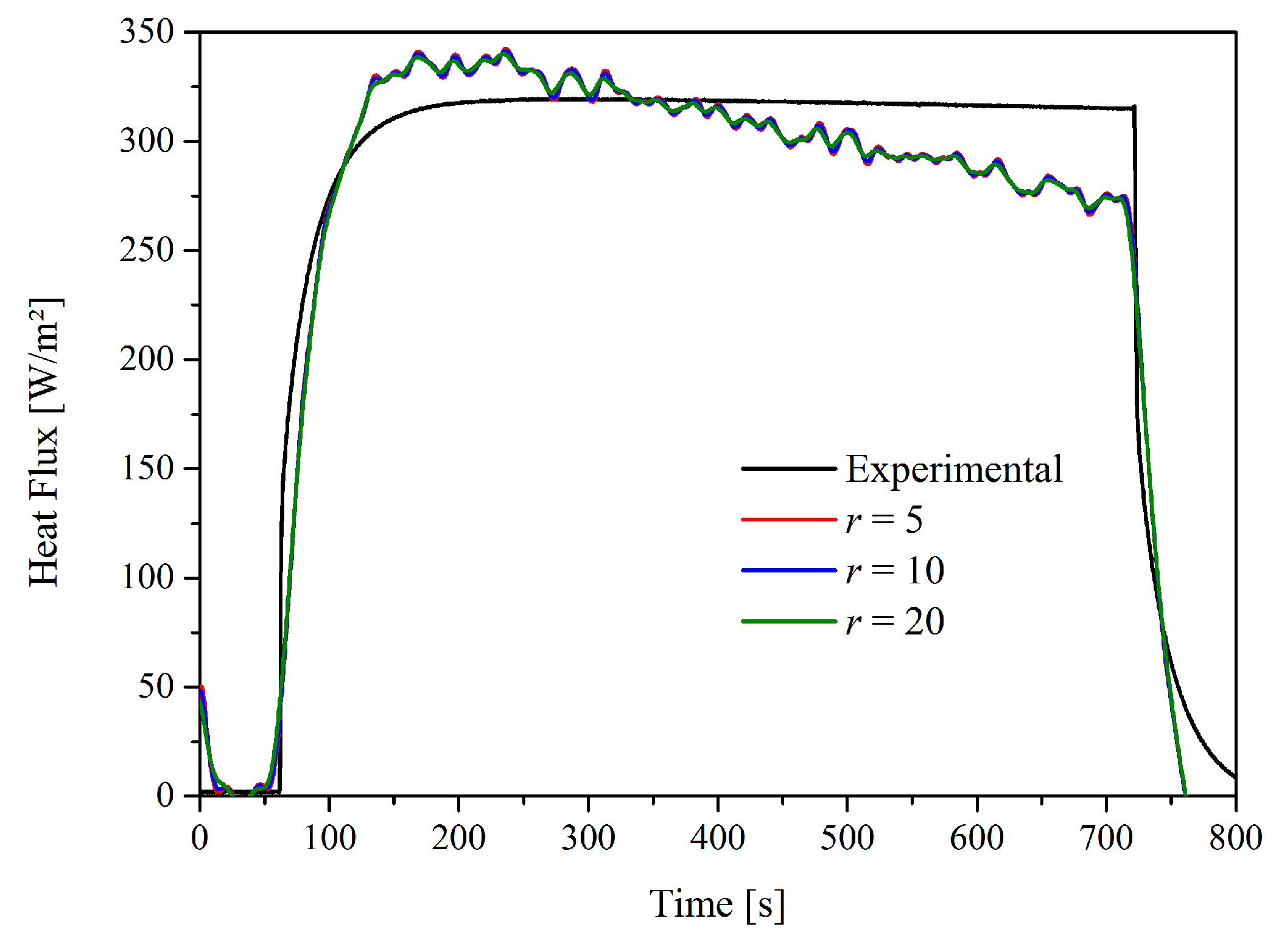
Figure 7.
(a) TTR, SFSM and experimental heat flux, (b) Difference of heat flux estimated using SFSM and TTR.
Figure 7.
(a) TTR, SFSM and experimental heat flux, (b) Difference of heat flux estimated using SFSM and TTR.

Figure 8.
Comparison between the experimental and calculated temperatures.

Figure 9.
Temperature residuals for both methods.

Figure 10.
Estimated heat flux for the AISI 304 stainless steel.

Figure 11.
Estimated heat flux for r = 60.

Figure 12.
Comparison between the experimental and numerical temperatures for r = 60 with TTR.

© 2018 by the authors. Licensee MDPI, Basel, Switzerland. This article is an open access article distributed under the terms and conditions of the Creative Commons Attribution (CC BY) license (http://creativecommons.org/licenses/by/4.0/).
Share and Cite
MDPI and ACS Style
Magalhães, E.D.S.; Anselmo, B.D.C.S.; Lima e Silva, A.L.F.d.; Lima e Silva, S.M.M. Time Traveling Regularization for Inverse Heat Transfer Problems. Energies 2018, 11, 507. https://doi.org/10.3390/en11030507
AMA Style
Magalhães EDS, Anselmo BDCS, Lima e Silva ALFd, Lima e Silva SMM. Time Traveling Regularization for Inverse Heat Transfer Problems. Energies. 2018; 11(3):507. https://doi.org/10.3390/en11030507
Chicago/Turabian StyleMagalhães, Elisan Dos Santos, Bruno De Campos Salles Anselmo, Ana Lúcia Fernandes de Lima e Silva, and Sandro Metrevelle Marcondes Lima e Silva. 2018. "Time Traveling Regularization for Inverse Heat Transfer Problems" Energies 11, no. 3: 507. https://doi.org/10.3390/en11030507
Note that from the first issue of 2016, this journal uses article numbers instead of page numbers. See further details here.