A Graph-Based Power Flow Method for Balanced Distribution Systems


1
School of Information and Electrical Engineering, Zhejiang University City College, Hangzhou 310030, China
2
College of Control Science and Engineering, Zhejiang University, Hangzhou 310027, China
3
College of Electrical Engineering, Zhejiang University, Hangzhou 310027, China
*
Author to whom correspondence should be addressed.
†
These authors contributed equally to this work.
Energies 2018, 11(3), 511; https://doi.org/10.3390/en11030511
Submission received: 14 December 2017
/
Revised: 21 February 2018
/
Accepted: 21 February 2018
/
Published: 27 February 2018
Abstract
:A power flow method based on graph theory is presented for three-phase balanced distribution systems. The graph theory is used to describe the power network and facilitate the derivation of the relationship between bus Currents and the bus Voltage Bias from the feeder bus (the CVB equation). A distinctive feature of the CVB equation is its unified form for both radial and meshed networks. The method requires neither a tricky numbering and layering of nodes nor breaking meshes and loop-analysis, which are both necessary in previous works for meshed networks. The convergence of the proposed method is proven using the Banach fixed-point theorem.
1. Introduction
Power flow calculation is the most fundamental numerical problem for power system analysis. A fast and general power flow method will be required by distribution systems as the development of smart grid and must be as efficient as possible in the future [1]. Methods on transmission networks are well developed such as Gauss–Seidel, Newton–Raphson [2] and Fast-Decoupled method [3]. Distribution networks have some special characteristics such as radial/weakly meshed structure, high R/X ratios of impedances, large number of branches and nodes, etc. These features may cause problems when the algorithms for power flow of transmission networks are applied to distribution systems [4]. Power flow calculations may be executed every five minutes on traditional networks, but as for microgrids, it may not meets the requirements. Microgrids have the natures of uncertainty and volatility, so they need real-time monitoring to guarantee their reliability, and require a faster power flow method. Power flow method is also a very important tool for improving the reliability and efficiency of fault analysis [5], and it can also provide evidence for protection for power distribution systems.
Backward/forward sweep (BFS) method ,which is intended to solve unbalanced radial distribution networks, has a very good performance, where all nodes are labeled into different layers according to distances from the feeder node. The branch currents are calculated in the backward sweep, while the bus voltage is then calculated in the forward sweep [6]. However, the BFS method cannot be applied directly to networks even with weakly meshed structure because the distances from the feeder node are not unique in the presence of loops. Shirmohammadi et al. have proposed a compensation-based power flow method for solving weakly meshed networks by using the multi-port compensation technique and basic formulations of Kirchhoff’s laws [7]. Teng has proposed a direct method for both radial and meshed networks by developing the bus-injection to branch-current (BIBC) matrix and the branch-current to bus-voltage (BCBV) matrix. However, when solving meshed networks, the method has to apply some preliminary operations, including Kron’s Reduction and modifying the two matrices by loop-analysis [8]. Wu and Zhang developed a power flow method for dealing with meshed network based on compensation and loop-analysis [9]. These methods all need extra processing for meshed networks.
This paper proposes a graph-based power flow method for distribution systems, which has a unified formulation for both radial and meshed networks. Compared with previous works, the method uses graph theory to directly build the CVB equation, a map to the bus currents from the bus voltage bias from the feeder node. It requires neither a tricky numbering and layering of nodes nor breaking meshes and loop-analysis, which are both necessary in previous works for meshed networks. Although graph theory has been used for power systems in many aspects [10,11,12], there are a few in power flow calculation. The most relevant is the work published more recently [13], where graph theory is used for building the Z-bus matrix, and the results obtained are only for radial distribution systems. The other contribution of this paper is that the convergence of the graph-based method is addressed by using the Banach fixed-point theorem, associated with the convergence rate of a clear physical meaning.
Notations: The following notations are used in this paper:
- CVB: The equation between the bus currents and the bus voltage bias from the feeder bus.
- BFS: The backward/forward sweep method.
- BIBC, BCBV: The bus-injection to branch-current matrix and the branch-current to bus-voltage matrix in [8].
- denote the rational, complex number sets.
- denotes the conjugate operator of complex number.
- : The inject current and voltage vectors of all nodes including the feeder node.
- : The inject current and voltage vectors of all nodes except the feeder node.
- : The voltage drop, impedance, current vectors of all branches.
- : Matrices of all impedance of branches/complex power of nodes except feeder node.
- : The incidence matrix with/without the row of feeder node.
- : The voltage difference vector between the feeder node and other nodes.
- : The mapping between and .
- : A —order vector with all elements being 1.
2. Problem Formulation
2.1. Topological Description of the Network
A distribution network has a typical tree structure, the root of which is the feeder node with a known voltage. Sometimes there are some extra branches between nodes so as to form a meshed structure.
We use undirected graph to depict the topology structure of a given distribution network where and are node set and branch set, respectively. If there is a branch between two nodes in a graph, the two nodes are connected. Although incidence matrix has been used in previous studies [14,15], it has to be numbered from front to back in sequence. By using of graph theory, we can give an arbitrary numbering to nodes and branches. Figure 1 shows two simple typical distribution network containing 4 nodes, where the feeder node is node 3, not the first node. Without loss of generality, the positive direction of branch current is defined to be always flowing out of the node with the lower number. In this setting, the incidence matrix of the graph is defined as
The incidence matrices of networks in Figure 1, for instance, are given as
Specially, for radial networks. It is rational to assume that the considered network is connected, which implies that the rank of H is .
2.2. Basic Formulations of Kirchhoff’s Laws
The power flow is related to the steady-state behavior of the power systems, where all the voltages and currents are sinusoidal signals with the same frequency. For a three-phase balanced distribution system, each signal can be represented by a complex value. Without loss of generality, all the electrical variables are complex numbers in this paper if not specifically stated.
In this sense, the current, voltage and complex power of node k are denoted by complex numbers , and , respectively. The positive direction of injects to node k, as illustrated in Figure 1. The concatenated current and voltage vectors are denoted by and . Let f be the number of feeder node. The feeding power of distribution networks can be given by , where denotes the conjugate operator.
Let , and be the current, voltage and impedance of branch k, respectively. The positive directions of and follow that of , i.e., from the node with lower number to the node with larger number. Similarly and . The diagonal impedance matrix is defined by .
Clearly one has
and
The Kirchhoff’s Current and Voltage Laws can be conveniently described by use of incidence matrix, respectively,
and they are valid for both radial and meshed networks. Combining with Equation (2), it follows that
2.3. Reformulation of Power Flow Equations
Equations (1) and (4) form the power flow equations. However, matrix is singular, which hampers constructing an identity map from them (an identity map is a function that always returns the same value that was used as its argument.).
For a distribution network, the feeder node is a slack node, whose voltage is fixed as the base value . This paper addresses the case that all the other buses except for the feeder bus are modeled as bus. Such a constant power case is increasingly common in the modern distribution systems because more and more power electronics devices are used.
Given the feeder node voltage and the complex power for other nodes , where notation denotes the subset of deleting the element f, the goal of power flow is to calculate the currents and voltages of nodes in the set , which we use to denote respectively, that is,
Correspondingly, let be the matrix removing the f-th row of H, with which
As for the examples in Figure 1, node 3 is the feeder node, then
Denote by the voltage differences between the feeder node and other nodes, namely,
Throughout of this paper, notation denotes a —order vector with all elements being 1. Due to , the following can be obtained,
3. Main Results
3.1. Review BFS Method
Traditional BFS method generally takes advantage of the radial topology. It starts with numbering and layering from the feeder node to terminal nodes. The backward sweep, starting from the terminal layer and ending at the first layer, is to calculate the branch currents by a current summation with a possible voltage update. The forward sweep operating in an opposite direction is to calculate the voltage drop of nodes with the branch currents obtained in the backward process.
Note that is nonsingular in a connected radial network, we can directly obtain branch current from by Equation (6), instead of by current summations in the backward sweep. In our study, the backward and forward processes can be described, based on graph theory, simply without layering as:
- (s1)
- ,
- (s2)
- ,
- (s3)
- ,
- (s4)
- ,
- (s5)
- ,
- (s6)
- repeat (s1) to (s5) until ,
where superscript denotes the values at the k-th iteration and is the convergence tolerance.
3.2. Unified Method for both Radial and Meshed Networks
The above graph-based process is no longer applicable for meshed network because is not a square matrix for meshed structure. The traditional methods cannot apply either in that the presence of circulating current prohibits layering nodes.
Generally, radial and meshed networks are dealt with separately when we consider the power flow for distribution systems. For dealing with meshed networks, breaking meshes or loop-analysis were needed in previous studies. Below, a uniform method for both radial and meshed networks is presented.
Here, is nothing but the Laplacian matrix weighted by branch admittances of removing the row and column corresponding to the feeder node. For a connected network, is always nonsingular no matter if is a square matrix. Define
Equation (10) builds a bijective mapping between and , by which the function of the steps (s2)–(s4) in BFS method can be compactly rewritten as
which is nothing but the CVB equation. Equations (10) and (12) look significant by themselves since they mean that the injected currents of nodes could be directly related not to node powers but to the node voltage bias from the feeder node.
Now, our uniform graph-based method now can be delivered as follows:
- (g1)
- ,
- (g2)
- ,
- (g3)
- ,
- (g4)
- Repeat (g1) to (g3) until .
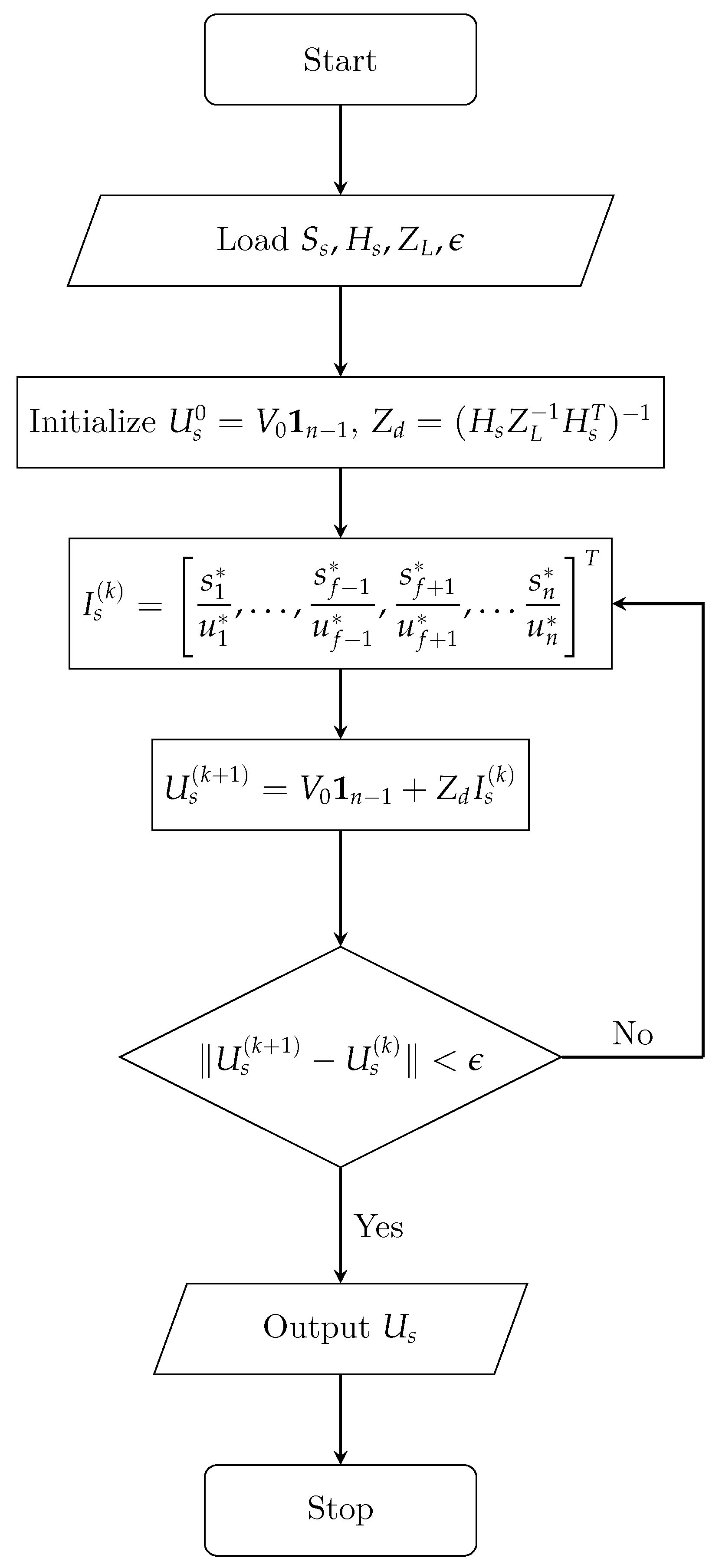
The initial value is generally set as . Note that the inversion of , i.e., does not need to calculate during the iteration. The flowchart of graph-based method is shown in Figure 2.
3.3. Convergence of Method
Since the above algorithm is explicit about the involved electrical variables, its convergence can be analyzed by using Banach fixed-point theorem.
Let , the diagonal matrix of injected power for node set . Denote by a vector consisting of all indexed by except for the fth one. Let be the solution of power flow, i.e., the steady state of the algorithm, and be the element of with the minimal magnitude, i.e., where is the ith element of .
Theorem 1.
Algorithm (g1)–(g4) is stable for all initial value satisfying
where
Proof.
The proposed algorithm is a mapping from to itself which essentially is a kind of fixed-point iteration and can be rewritten as
Based onBanach fixed-point theorem, the fixed-point satisfying exists and is unique if is a contraction mapping on . It can be seen that
where with .
Due to , one has and for all . Subsequently for one . Furthermore, for all . Therefore, due to Equation (13),
which implies that . It together with the initial condition shows that is a contraction mapping on . ☐
Remark 1.
The condition in Equation (14) implies that and .
Remark 2.
A smaller will lead to a larger R. This implies roughly that a strong network (a small ratio between transmitted power and the branch admittance, ) allows a large permissible region for direct approaches of power flow. Meanwhile a small means a small Lipschitz constant and subsequently a fast convergence.
3.4. Comparison to the Direct Approach
It can be seen that our Algorithm (g1)–(g3) is similar to that in [8]. This is not surprising, in that both are based on Equation (12), the mapping from to . The difference is how to obtain Equation (12). The distinctive feature of our graph-based method is to present a much simpler way than the direct approach in [8].
Recall the CVB equation obtained by the direct approach [8] as: for radial networks,
and for meshed networks,
followed by a Kron’s Reduction. The following comparison is stated.
In the radial network, the direct approach needs: (1) sequentially numbering nodes and edges from layer to layer beginning at the feeder node; (2) performing a six-step algorithmto build the matrices (BCBV) and (BIBC) ; and (3) obtaining by multipling (BCBV) by (BIBC). Our method needs: (1) an arbitrary numbering nodes and edges; (2) directly writing matrices H, , and ; and (3) calculating .
In the meshed network, the direct approach needs an extra drawing the corresponding radial version of the meshed network, adding two steps for every extra branch that makes the network meshed to build matrices (BCBV) and (BIBC), and a Kron’s reduction.
Thus, the complexity of the direct approach would increase largely as the degree of mesh increases, while our method has the same procedure for the meshed network as that for the radial network. In fact, our method can apply to any meshed network rather than to the weakly-meshed network. Moreover, our method has a clearer physical meaning because no network reduction has to be made. The above contents are summarized in Table 1 for a clear insight.
4. Test Results
The proposed method is tested and compared on both radial and meshed networks on MATLAB. Table 2 shows the distribution systems of 14-, 33-, 69-, 84-, 119-, 135-, and 874-node radial networks and their meshed editions, which are from papers [16,17,18,19,20].
Four methods are tested. Method I is the Gauss–Seidel Method, Method II is the Newton–Raphson method, Method III is the direct approach proposed in [8] and Method IV is our Graph-based method. The convergence tolerance is set at 0.001 p.u.
Table 3 and Table 4 show the performance of these four methods for radial and meshed networks, where “Time” and “ITs” denote the iteration time and iteration numbers, respectively, and “L” denotes the approximate Lipschitz constant, which describes the convergence rate of Method IV. According to the tables, Method I, the Gauss–Seidel method, costs much more time and iteration steps than the three other methods, since it has a very low convergence rate so that even if it does not need much time at each iteration, it still costs much time. Method II, the Newton–Raphson method, needs fewer iteration steps than other methods since it follows the direction of gradient descent at every step. However, the Newton–Raphson method still costs more time than Method III and IV, because it requires calculating the Jacobian matrix and its inversion matrix at each iteration, which costs majority of time. Therefore, the time consumption of Newton–Raphson is more related to the number of nodes compared with Method III and IV.
As for Method III and Method IV, the results show the direct approach is approximately equivalent to the proposed method, which is consistent with the theoretical analysis. However, the advantage of our method is the process to get the CVB equation. As mentioned above, the direct approach requires loop-analysis and Kron’s Reduction for meshes networks, while our method does not need any extra processing. Table 5 provides a comparison of time spent on getting the CVB equation, and the result shows that the proposed method takes less time than the direct approach to get the CVB equation. Moreover, for the example of the 14-node network, we only increase the number of mesh, and the results show that the time consumptions of proposed method are almost the same when the number of meshes increased, unlike the increasing time consumptions of direct approach, mainly due to the Kron’s Reduction. Note that, in the case that the node numbering, the radial structure drawing and the meshed branch identifying have been made in advance, it can be seen that the graph-based method is much better if the time spent on these pretreatments are contained.
Limitations
The proposed method has shown obvious advantage compared to previous works. However, it has some limitations. First, as for the impact of distributed generators, DGs can be considered as nodes with constant active/reactive powers as well as nodes with constant active power and voltage magnitude. If DGs are considered as nodes, our method can deal with it. Alternatively, if DGs are considered as PV nodes, our method is not applicable. Besides, as for the applicability to unbalanced networks, we have a preliminary outline to extend our method for unbalanced networks, but the work still needs deliberate discussion and proof. Finally, the impact of FACTS devices is not discussed in this paper since FACTS devices cannot be simply modeled as nodes and our method aims at distribution networks with nodes.
5. Conclusions
This paper has proposed a graph-based power flow method for three-phase balanced distribution systems with nodes. For the nature of distribution systems such as radial/weakly meshed structure, and large number of branches and nodes, traditional power flow method may fail or cannot meet the requirement. With regards to this, we have made some progress. The proposed method provides a uniform formulation for both radial and meshed networks. The uniform formulation is much simpler than before, requiring neither a tricky numbering and layering of nodes nor breaking meshes and loop-analysis, which are both necessary in previous works for meshed networks. The convergence of the proposed method has been shown by using the Banach fixed-point theorem. The comparison test results show the efficiency of our competitive method.
Acknowledgments
The authors would like to thank anonymous reviewers for their valuable comments and insights. This research was supported by the National key research and development program of China (2016YFB0900605), the National Natural Science Foundation of China(61573314, 61773339), the science and technology project of SGCC(5211SX16000J).
Author Contributions
Tao Shen conducted analysis and simulations. Yanjun Li provided guidance, conception and gave final approval of the version to be submitted. Ji Xiang provided guidance, conception and plan.
Conflicts of Interest
The authors declare no conflict of interest.
References
- Balamurugan, K.; Srinivasan, D. Review of power flow studies on distribution network with distributed generation. In Proceedings of the 2011 IEEE Ninth International Conference on Power Electronics and Drive Systems (PEDS), Singapore, 5–8 December 2011; pp. 411–417. [Google Scholar]
- Nguyen, H.L. Newton-Raphson Method in Complex Form. IEEE Trans. Power Syst. 1997. [Google Scholar] [CrossRef]
- Zimmerman, R.D.; Chiang, H.D. Fast decoupled power flow for unbalanced radial distribution systems. IEEE Trans. Power Syst. 1995, 10, 2045–2052. [Google Scholar] [CrossRef]
- Luo, G.X.; Semlyen, A. Efficient load flow for large weakly meshed networks. IEEE Trans. Power Syst. 1990, 5, 1309–1316. [Google Scholar] [CrossRef]
- Ou, T.C. A novel unsymmetrical faults analysis for microgrid distribution systems. Int. J. Electr. Power Energy Syst. 2012, 43, 1017–1024. [Google Scholar] [CrossRef]
- Kersting, W.H. A Method to Teach the Design and Operation of a Distribution System. IEEE Trans. Power Appar. Syst. 1984, 7, 1945–1952. [Google Scholar] [CrossRef]
- Shirmohammadi, D.; Hong, H.W.; Semlyen, A.; Luo, G.X. A compensation-based power flow method for weakly meshed distribution and transmission networks. IEEE Trans. Power Syst. 1988, 3, 753–762. [Google Scholar] [CrossRef]
- Teng, J.H. A direct approach for distribution system load flow solutions. IEEE Trans. Power Deliv. 2003, 18, 882–887. [Google Scholar] [CrossRef]
- Wu, W.C.; Zhang, B.M. A three-phase power flow algorithm for distribution system power flow based on loop-analysis method. Int. J. Electr. Power Energy Syst. 2008, 30, 8–15. [Google Scholar] [CrossRef]
- De, M.; Goswami, S.K. A Direct and Simplified Approach to Power-flow Tracing and Loss Allocation Using Graph Theory. Electr. Power Compon. Syst. 2010, 38, 241–259. [Google Scholar] [CrossRef]
- Mehta, D.; Ravindran, A.; Joshi, B.; Kamalasadan, S. Graph theory based online optimal power flow control of Power Grid with distributed Flexible AC Transmission Systems (D-FACTS) Devices. In Proceedings of the North American Power Symposium, Charlotte, NC, USA, 4–6 October 2015; pp. 1–6. [Google Scholar]
- Pan, L.; Liu, J.; Cheng, P.; Wang, D. Fast Recognition of Power Flow Transferring Under Change of Power Network Topology. Power Syst. Technol. 2011, 35, 118–121. [Google Scholar]
- Hsieh, T.Y.; Chen, T.H.; Yang, N.C. Matrix decompositions-based approach to Z-bus matrix building process for radial distribution systems. Int. J. Electr. Power Energy Syst. 2017, 89, 62–68. [Google Scholar] [CrossRef]
- Yang, N.C. Three-phase power flow calculations by direct ZLOOP method for microgrids with electric vehicle charging demands. IET Gener. Transm. Distrib. 2013, 7, 1002–1010. [Google Scholar] [CrossRef]
- Yang, N.C. Three-phase power flow calculations using direct Z BUS method for large-scale unbalanced distribution networks. IET Gener. Transm. Distrib. 2016, 10, 1048–1055. [Google Scholar] [CrossRef]
- Baran, M.E.; Wu, F.F. Network reconfiguration in distribution systems for loss reduction and load balancing. IEEE Trans. Power Deliv. 1989, 4, 1401–1407. [Google Scholar] [CrossRef]
- Savier, J.S.; Das, D. Impact of Network Reconfiguration on Loss Allocation of Radial Distribution Systems. IEEE Trans. Power Deliv. 2007, 22, 2473–2480. [Google Scholar] [CrossRef]
- Su, C.T.; Lee, C.S. Network Reconfiguration of Distribution Systems Using Improved Mixed-Integer Hybrid Differential Evolution. IEEE Power Eng. Rev. 1989, 22, 66. [Google Scholar] [CrossRef]
- Civanlar, S.; Grainger, J.J.; Yin, H.; Lee, S.S.H. Distribution feeder reconfiguration for loss reduction. IEEE Trans. Power Deliv. 1988, 3, 1217–1223. [Google Scholar] [CrossRef]
- Zhang, D.; Fu, Z.; Zhang, L. An improved TS algorithm for loss-minimum reconfiguration in large-scale distribution systems. Electr. Power Syst. Res. 2007, 77, 685–694. [Google Scholar] [CrossRef]
Figure 1.
A typical radial network and meshed network: (a) radial structure (, ); and (b) meshed structure (, ).
Figure 1.
A typical radial network and meshed network: (a) radial structure (, ); and (b) meshed structure (, ).
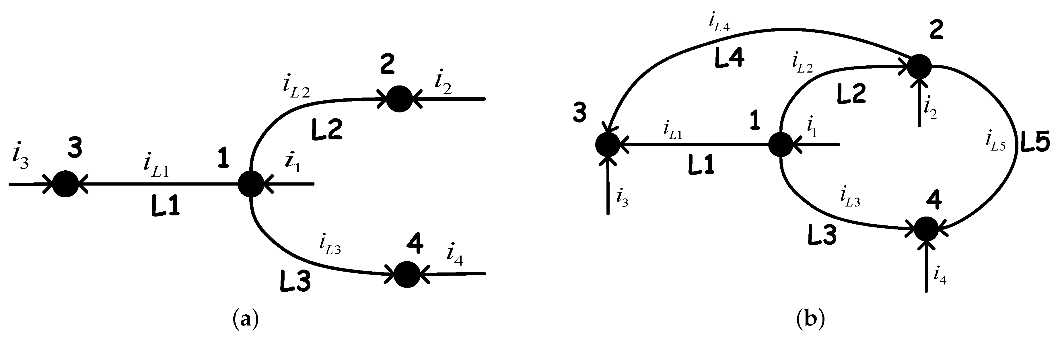
Figure 2.
The flowchart of graph-based method.

Table 1.
Comparison with Direct Approach.
| Radial Networks | ||
| Direct Approach | Proposed Method | |
| Numbering | Sequential | Arbitrary |
| Matrices | ||
| Operation | ||
| Meshed Networks | ||
| Direct Approach | Proposed Method | |
| Meshes | Need Recognition | No Need |
| Numbering | Sequential for radial structure and place meshes to the end | Arbitrary |
| Matrices | Modified | |
| Operation | Modifying and Applying Kron’s Reduction | |
Table 2.
Network Configuration.
| No. of Nodes | No. of Branch (Radial) | No. of Branch (Meshed) |
|---|---|---|
| 14 | 13 | 16 |
| 33 | 32 | 37 |
| 69 | 68 | 73 |
| 84 | 83 | 96 |
| 119 | 118 | 132 |
| 135 | 134 | 156 |
| 874 | 873 | 900 |
Table 3.
Radial Network Test.
| No. of Nodes | Method I | Method II | Method III | Method IV | |||||
|---|---|---|---|---|---|---|---|---|---|
| Time | ITs | Time | ITs | Time | ITs | Time | ITs | L | |
| 14 | 7.7 × 10⁻³ | 25 | 5.2 × 10⁻⁴ | 2 | 1.2 × 10⁻⁵ | 2 | 1.1 × 10⁻⁵ | 2 | 0.012 |
| 33 | 0.31 | 433 | 1.2 × 10⁻³ | 3 | 2.5 × 10⁻⁵ | 4 | 2.5 × 10⁻⁵ | 4 | 0.091 |
| 69 | 0.75 | 476 | 2.4 × 10⁻³ | 3 | 3.7 × 10⁻⁵ | 4 | 3.6 × 10⁻⁵ | 4 | 0.17 |
| 84 | 0.7 | 353 | 3.8 × 10⁻³ | 3 | 4.4 × 10⁻⁵ | 4 | 4.4 × 10⁻⁵ | 4 | 0.097 |
| 119 | 1.4 | 493 | 5.7 × 10⁻³ | 3 | 7.6 × 10⁻⁵ | 4 | 7.5 × 10⁻⁵ | 4 | 0.14 |
| 135 | 1.7 | 519 | 6.0 × 10⁻³ | 3 | 6.5 × 10⁻⁵ | 3 | 6.6 × 10⁻⁵ | 3 | 0.091 |
| 874 | 0.78 | 27 | 0.67 | 3 | 4.0 × 10⁻³ | 4 | 4.0 × 10⁻³ | 4 | 0.056 |
Table 4.
Meshed Network Test.
| No. of Nodes | Method I | Method II | Method III | Method IV | |||||
|---|---|---|---|---|---|---|---|---|---|
| Time | ITs | Time | ITs | Time | ITs | Time | ITs | L | |
| 14 | 8.6 × 10⁻³ | 30 | 5.3 × 10⁻⁴ | 2 | 1.2 × 10⁻⁵ | 2 | 1.1 × 10⁻⁵ | 2 | 7.5 × 10⁻³ |
| 33 | 0.16 | 220 | 1.2 × 10⁻³ | 3 | 1.9 × 10⁻⁵ | 3 | 1.9 × 10⁻⁵ | 3 | 0.05 |
| 69 | 0.28 | 178 | 3.0 × 10⁻³ | 3 | 2.7 × 10⁻⁵ | 3 | 2.7 × 10⁻⁵ | 3 | 0.066 |
| 84 | 0.65 | 336 | 3.0 × 10⁻³ | 3 | 3.4 × 10⁻⁵ | 3 | 3.3 × 10⁻⁵ | 3 | 0.059 |
| 119 | 0.78 | 283 | 4.8 × 10⁻³ | 3 | 5.7 × 10⁻⁵ | 3 | 5.6 × 10⁻⁵ | 3 | 0.061 |
| 135 | 1.6 | 504 | 6.1 × 10⁻³ | 3 | 6.5 × 10⁻⁵ | 3 | 6.6 × 10⁻⁵ | 3 | 0.028 |
| 874 | 0.5 | 17 | 0.45 | 2 | 2.0 × 10⁻³ | 2 | 2.1 × 10⁻³ | 2 | 7.9 × 10⁻³ |
Table 5.
Time to get the CVB equation.
| No. of Node | No. of Branch | Method IV Time | Method III Time |
| 14 | 16 | 5.5 × 10⁻⁵ | 1.2 × 10⁻⁴ |
| 33 | 37 | 1.3 × 10⁻⁴ | 2.6 × 10⁻⁴ |
| 69 | 73 | 3.9 × 10⁻⁴ | 6.4 × 10⁻⁴ |
| 84 | 96 | 5.2 × 10⁻⁴ | 9.2 × 10⁻⁴ |
| 119 | 132 | 8.2 × 10⁻⁴ | 1.4 × 10⁻³ |
| 135 | 156 | 1.1 × 10⁻³ | 1.8 × 10⁻³ |
| 874 | 900 | 9.5 × 10⁻² | 1.1 × 10⁻¹ |
| No. of Node | No. of Branch | Method IV Time | Method III Time |
| 14 | 3 | 5.5 × 10⁻⁵ | 1.2 × 10⁻⁴ |
| 14 | 4 | 5.5 × 10⁻⁵ | 1.5 × 10⁻⁴ |
| 14 | 5 | 5.5 × 10⁻⁵ | 1.7 × 10⁻⁴ |
| 14 | 6 | 5.5 × 10⁻⁵ | 2.5 × 10⁻⁴ |
| 14 | 7 | 5.6 × 10⁻⁵ | 2.6 × 10⁻⁴ |
| 14 | 8 | 5.6 × 10⁻⁵ | 2.6 × 10⁻⁴ |
| 14 | 9 | 5.6 × 10⁻⁵ | 2.7 × 10⁻⁴ |
© 2018 by the authors. Licensee MDPI, Basel, Switzerland. This article is an open access article distributed under the terms and conditions of the Creative Commons Attribution (CC BY) license (http://creativecommons.org/licenses/by/4.0/).
Share and Cite
MDPI and ACS Style
Shen, T.; Li, Y.; Xiang, J. A Graph-Based Power Flow Method for Balanced Distribution Systems. Energies 2018, 11, 511. https://doi.org/10.3390/en11030511
AMA Style
Shen T, Li Y, Xiang J. A Graph-Based Power Flow Method for Balanced Distribution Systems. Energies. 2018; 11(3):511. https://doi.org/10.3390/en11030511
Chicago/Turabian StyleShen, Tao, Yanjun Li, and Ji Xiang. 2018. "A Graph-Based Power Flow Method for Balanced Distribution Systems" Energies 11, no. 3: 511. https://doi.org/10.3390/en11030511
Note that from the first issue of 2016, this journal uses article numbers instead of page numbers. See further details here.