A Reconfigured Whale Optimization Technique (RWOT) for Renewable Electrical Energy Optimal Scheduling Impact on Sustainable Development Applied to Damietta Seaport, Egypt

Abstract

This paper studies the effect on the rate of growth of carbon dioxide emission in seaports’ atmosphere of replacing a part of the fossil fuel electrical power generation by clean renewable electrical energies, through two different scheduling strategies. The increased rate of harmful greenhouse gas emissions due to conventional electrical power generation severely affects the whole global atmosphere. Carbon dioxide and other greenhouse gases emissions are responsible for a significant share of global warming. Developing countries participate in this environmental distortion to a great percentage. Two different suggested strategies for renewable electrical energy scheduling are discussed in this paper, to attain a sustainable green port by the utilization of two mutual sequential clean renewable energies, which are biomass and photovoltaic (PV) energy. The first strategy, which is called the eco-availability mode, is a simple method. It is based on operating the renewable electrical energy sources during the available time of operation, taking into consideration the simple and basic technical issues only, without considering the sophisticated technical and economical models. The available operation time is determined by the environmental condition. This strategy is addressed to result on the maximum available Biomass and PV energy generation based on the least environmental and technical conditions (panel efficiency, minimum average daily sunshine hours per month, minimum average solar insolation per month). The second strategy, which is called the Intelligent Scheduling (IS) mode, relies on an intelligent Reconfigured Whale Optimization Technique (RWOT) based-model. In this strategy, some additional technical and economical issues are considered. The studied renewable electrical energy generation system is considered in two scenarios, which are with and without storage units. The objective (cost) function of the scheduling optimization problem, for both scenarios, are developed. Also, the boundary conditions and problem constraints are concluded. The RWOT algorithm is an updated Whale Optimization Algorithm (WOA). It is developed to accelerate the rate of reaching the optimal solution for the IS problem. The two strategies simulation and implementation are illustrated and applied to the seaport of Damietta, which is an Egyptian port, located 10 km to the west of the Nile River (Damietta Branch). The scheduling of PV and biomass energy generation during the different year months is examined for both strategies. The impact of renewable electrical energies generation scheduling on carbon dioxide emission and consequently global warming is discussed. The saving in carbon dioxide emission is calculated and the efficient results of the suggested models are clarified. The carbon dioxide emission is reduced to around its fifth value, during renewable energy operation. This work focuses on decreasing the rate of growth of carbon dioxide emission coming from fossil fuel electrical power generation in Egypt, targeting, sustainable green seaports, through three main contributions in clean renewable electrical energies scheduling. The contributions are: 1-presenting the eco-availability mode for minimum gifted biomass and PV energy generation, 2-developing and progressing the IRWOT scheduling strategy for both scenarios (with and without storage unit), 3-defining the scheduling optimization problem boundary conditions and constraints.

1. Introduction

The great need to search for new environmental energy sources is increaseing, not only due to the expected shortage of conventional electrical energy resources, but also because of the increasing rate of pollution and harmful emissions. The concentration of heat-trapping greenhouse gases in the atmosphere has significantly increased throughout the preceding century as a result of burning fossil fuels, deforestation, and other causes. These gases act like a cover that make the world’s surface hotter than it ought to be the place as it captures a portion of the warmth emanated from the world’s surface and afterward this warmth is retransmitted back to the surface. Many publications concerned with Life Cycle Assessments of various electricity generation technologies have been performed throughout the past decades [1,2,3,4].

Within the electric power sector, assessments for the life cycle greenhouse gas “GHG” emissions for solar, wind, nuclear, and coal technologies showed that the total life cycle GHG emissions from fossil fuels are much higher and more variable than those from nuclear energy and other clean, renewable sources. Assessments showed that the generation of electricity from fossil fuel combustion is responsible for the vast majority of GHG emissions. For instance, electricity generated using coal-fired releases about 20 times more GHGs per kilowatt-hour than any clean, renewable energy sources whether it’s solar, wind or nuclear energy [1,2,3,4].

Carbon dioxide (CO₂) plays a remarkable part as the main GHG released from process of fossil fuels combustion. The atmospheric concentration of CO₂ has increased by over 40% from a preindustrial amount of 280 ppm (parts/million) to over 400 parts/million in 2016. With the increase of the CO₂ and GHGs concentrations, the universal average temperatures are growing [1,2,3].

Substitutional clean energy sources, replacing the conventional fossil fuels electrical energy resources, should be renewable to uphold the objective of sustainable development. Photovoltaic (PV) and biomass energies are clean and renewable electrical energy generation resources [5,6,7,8,9].

One of the noticeable renewable energy resources is biomass energy. Since the 1970s, some scientists became more interested in the possibility of replacing fossil fuels with biomass [10]. Around 1975, “biomass” became the formal name of this energy [10]. Although currently fulfillment of the majority of the energy needs and requirements is still attained through the combustion of fossil fuel, 14% of the world utilizes biomass. Generating energy could be attained through the thousands of tons of manure, mounds of agricultural waste and piles of sawdust.

In these days, around 7% of the yearly production of biomass is utilized worldwide. New technologies in biomass energy field are progressing, despite the little investment in biomass research. This small investment in the biomass area relegates biomass plants to small niche markets and individual efforts. These small-scale projects can become economically efficient and environmentally sustainable [11,12,13]. Nowadays, the thermal and/or the electrical returns of biogas are targeted in many researches. Despite the fact that the electrical power generation from biomass is considered to be a promising task, that research mainly focuses on the thermal energy section [6,14,15,16]. In biomass technology, the improvement of the exhaust quality and its contents from hydrogen and carbon faces has seen many updates through the years. Many techniques and approaches, targeting the enhancement of the generation and the reduction of the CO₂ are investigated in [17,18,19,20,21].

Lately, PV electrical power generation has been receiving considerable attention, especially, when a comparison is made with the traditional power systems. Thus, a PV system could be designed to fulfill the various requirements of applications and operations, through being either a stand-alone unit (distributed power generation) or connected to an electrical power grid. PV systems are static sunlight fuel systems, that avoid noise and pollution. PV modules have the capability of expanding and transporting in certain situations. In general, minimal maintenance is required for well-designed and properly installed PV systems, and additionally, they will have long-service lifetimes [5,7,8,9,12,13]. In 1952, the primal prototype is introduced [22]. During the 1970s, cost reduction was attained through the enhancements performed in manufacturing, performance, and quality of PV modules [23]. Following 1970s energy crisis, considerable efforts were progressed to develop PV power systems for both the commercial and residential utilizes, for stand-alone, remote power, and utility-connected applications. Solar energy harvesting technologies have progressed to exploit this almost unlimited energy utilization potential [24]. Recently, the PV module production industry is growing extensively. Implementation of PV systems on buildings and correlation to utility networks is accelerating rapidly in the major programs of Europe, Japan, and the USA [22,25,26]. Also, free software packages for PV electricity production allow quick estimations and calculations to be developed, discussed and compared [27]. Photovoltaic Geographical Information System (PVGIS), PVWatts and RETScreen are three major examples of these free software packages, which can help in PV system simulation and estimation.

One of the pivotal environmental entities that emits different types of contaminants which affect the total atmospheric pollution percentage is seaports. Many researches and projects address the sustainable green seaport technologies [28,29,30]. An ecological port (or green port) is a sustainable development port which is capable of both fulfilling the environmental requirements along with increasing their economic value. Creating a good ecological environment and high economic efficiency along with ensuring the overall harmonious and sustainable construction of the community’s economic, environmental complex ecosystem in the port is considered to be the main objective of the ecological port [31]. There are 15 commercial and 44 specialized ports on the Egyptian coast [32].

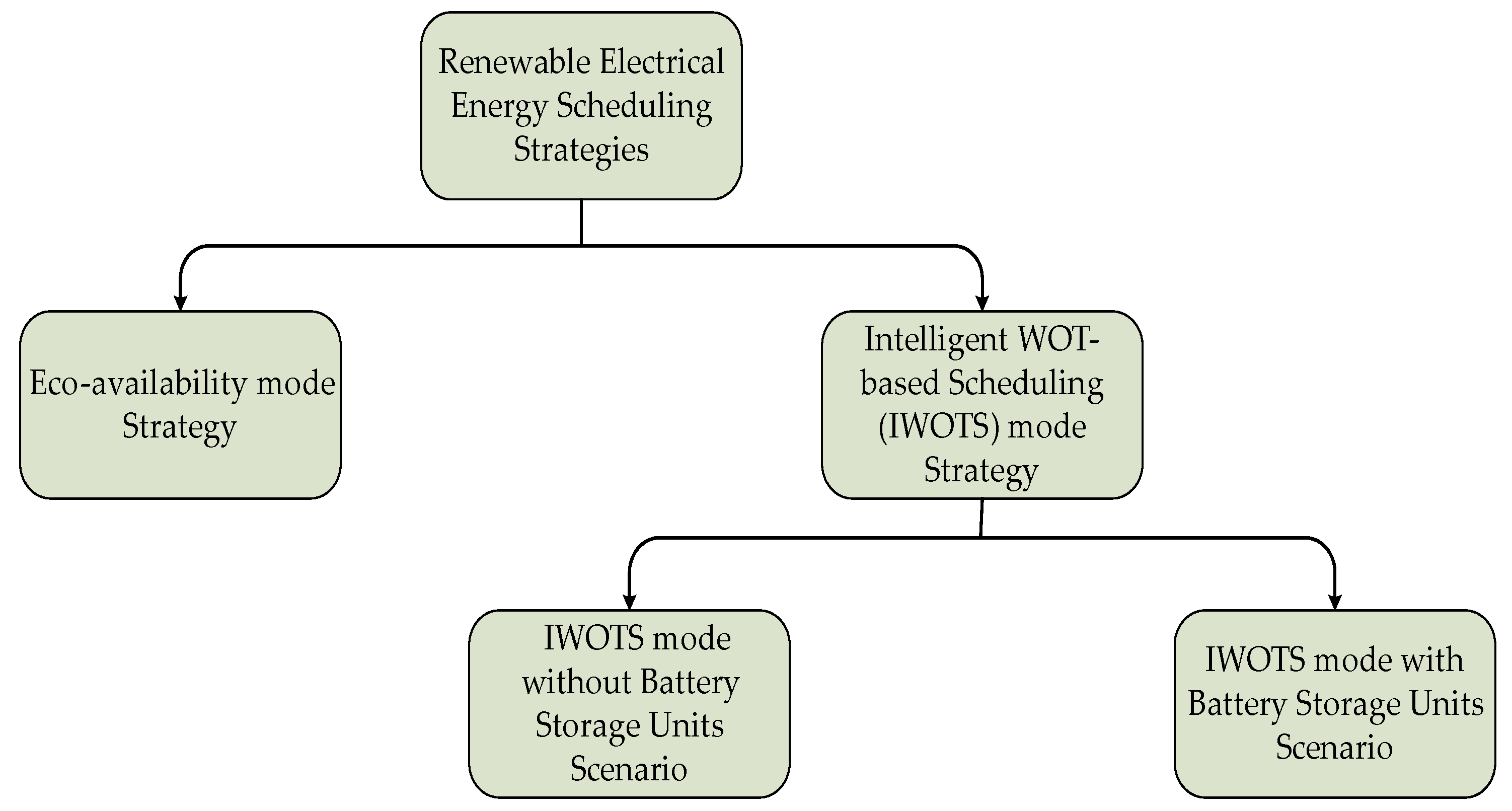
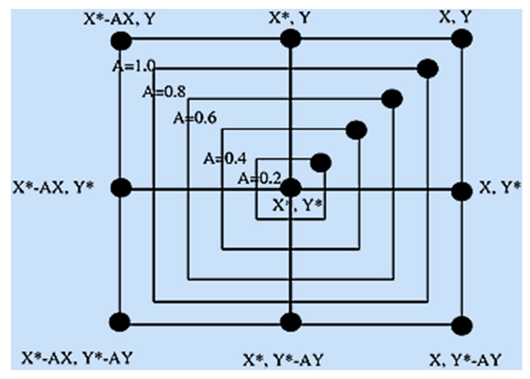
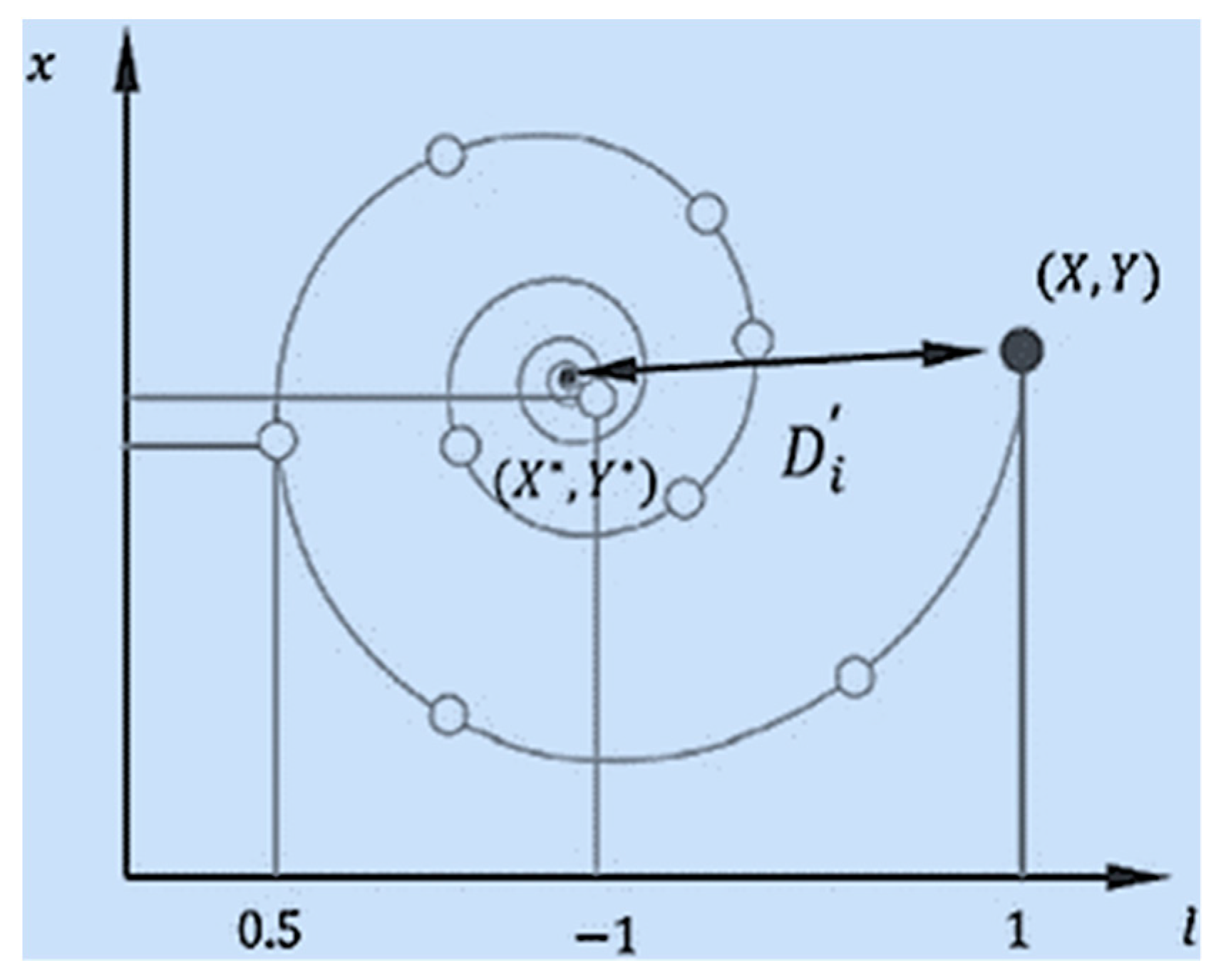
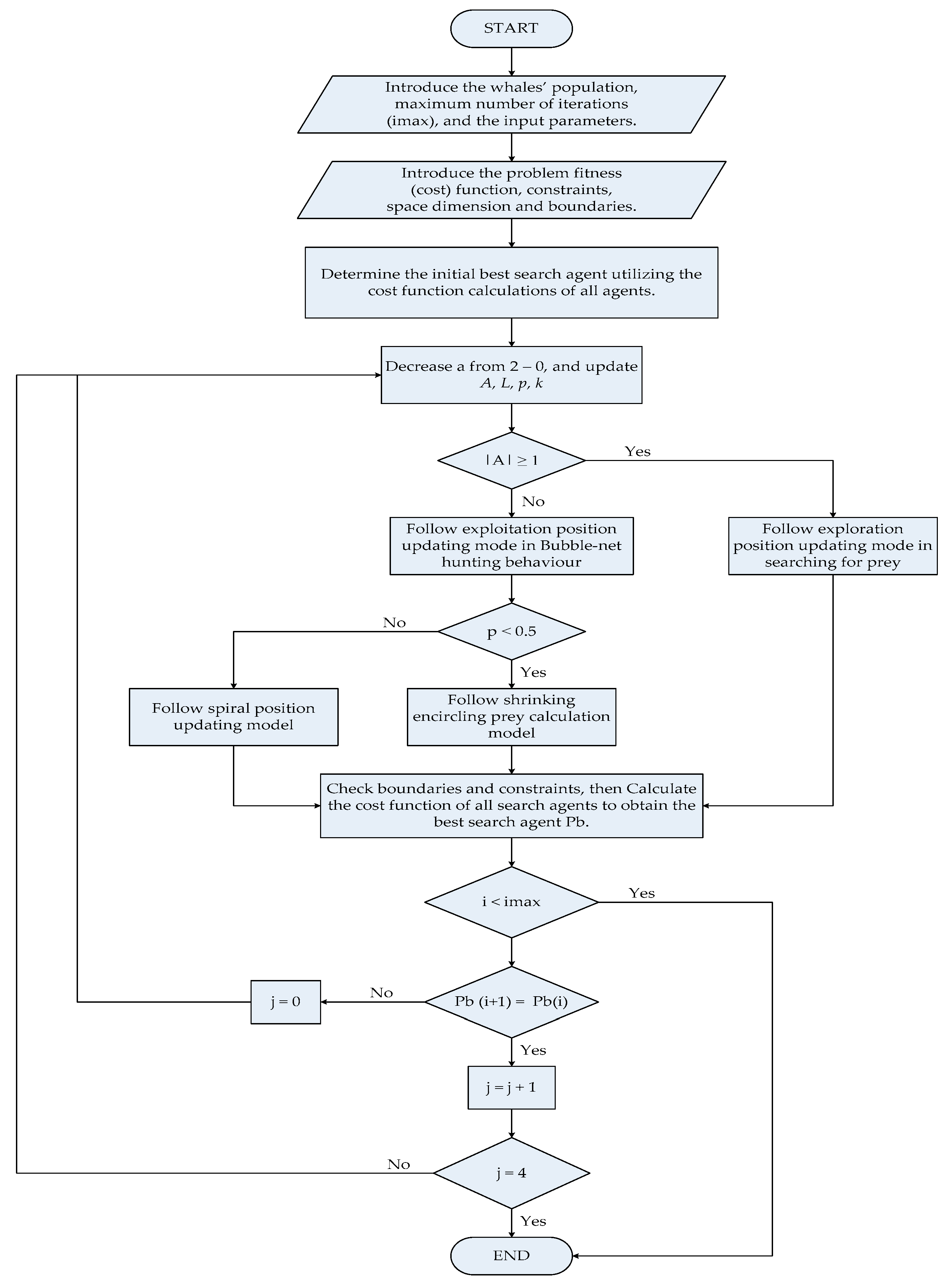
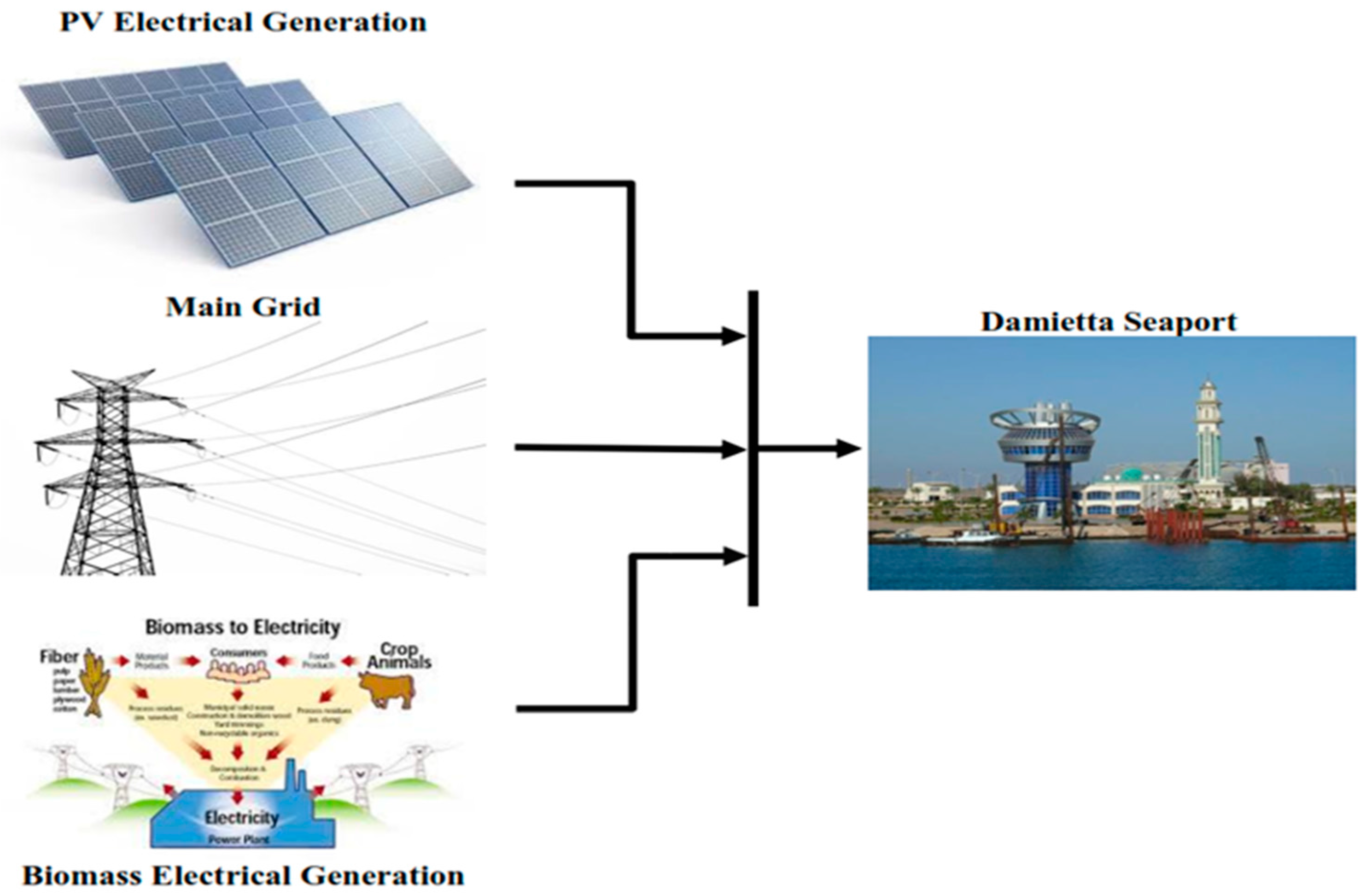
This paper discusses the impact of renewable electrical energy scheduling on carbon dioxide emission reduction through two strategies: (i) a port connected to the grid, which is called, eco-availability mode strategy and (ii) a standalone system which is called Intelligent Scheduling (IS) mode strategy (with and without storage unit consideration). Our eco-availability study is based on the basic technical-environmental (techno-env) operational availability conditions. The intelligent scheduling mode is an optimizing approach based on Reconfigured Whale Optimization Technique (RWOT) targeting the maximization the of carbon dioxide emission reduction. The RWOT cost function is derived in two cases, which are with and without considering the storage battery units. An integrated study is held for both strategies, regarding the environmental influences. The model of the green energy seaport is discussed and applied to one of the Egyptian seaports, which is the Damietta seaport.

The paper is divided into seven sections: Section 2 gives an overview of the environmental effects of carbon oxides. Section 3 provides an overview of biomass and photovoltaic general modeling and applications. The RWOT overview, algorithm description and the proposed cost function are illustrated in Section 4. Section 5 presents an integrated description for the proposed studied port (Damietta port). The simulation and results of both eco-availability strategy and IS strategy are clarified in Section 6, while Section 7 discusses the paper’s conclusions.

2. Carbon Oxides and Environmental Effect

2.1. Carbon Dioxide (CO₂)

With increased emissions of carbon dioxide, global warming will continue to increase, followed by rising sea levels due to melting polar ice, a slight increase in the average global rainfall in the twentieth century and the increase in the proportion of parts of the world exposed to waves of drought or flooding since 1970. Many scientists have warned of major changes that would affect marine life if no strong action is taken to reduce carbon dioxide emissions. Ocean temperatures are on the rise, and more oxygen is lost as salinity rises because of higher carbon dioxide, experts said. Many experts point out that many of the living organisms can withstand the future in front of rising temperatures because of carbon dioxide, but not every time [33,34,35,36].

The ocean is at the forefront of climate change with signs of a change in its physical and chemical system that ecosystems and organisms are already changing, and these changes will continue as long as the emissions continue. They warned that oceans have absorbed about 30 percent of the carbon dioxide produced by humans since 1750, and since carbon dioxide is acidic, it increases the salinity of seawater. Scientists say that high salinity rates are expected to affect reproduction, nutrition and marine growth rates.

2.2. Carbon Monoxide (CO)

Carbon monoxide is a poisonous gas that causes the death of a high-concentration product that exceeds the limit. The surrounding air is safe and uncontaminated if the carbon monoxide concentration is 5 parts per million (PPM). Carbon monoxide is colourless and odourless gas that results from the incomplete combustion of fuel. Its concentration varies in urban areas, depending on the conditions prevailing in each of these areas. It depends mainly on the intensity of traffic and therefore more concentrated in the day at night and affects the carbon monoxide on public health, especially on Hemoglobin blood as it has a strong susceptibility to union with it. It seriously affects the breathing processes in living organisms, including human and causes many poisoning cases [36,37,38]. Most organisms are at risk of carbon monoxide poisoning. The most affected are fetuses, children and people with heart and respiratory diseases, as well as anemia. Annual deaths from accidental poisoning by carbon monoxide in the United States are estimated at five hundred cases per year, while nearly 2000 people commit suicide by inhalation. The effects of exposure to different levels of carbon oxides have been reviewed [34,35,36].

3. Biomass and Photovoltaics

3.1. Biomass

Biomass is a substance that is structurally based on carbon [39]. Biogas is a form of energy produced by biochemically breaking down organic materials from biomass under anaerobic conditions [40]. Biogas is an ignitable gas, with an average calorific value of ca. 6 kWh/m³. Biogas production amount depends upon the processed chemical reaction different parameters. The type of the bio-waste and its Total Solids Percentage (TS %) are counted as reference to the effective parameters. Alcohol fermentation, landfill gas, and gasification are considered among the different techniques of biomass utilization. Gasification is the latest method for electricity generation. Gasification is based on capturing about 70% of the available energy extracted from solid fuels through a conversion process that turn the fuel into combustible-gases and then burning these gases, and generates energy. Synthetic fuel technologies (synfuel) are still new [11,12,13,14,15,41,42].

Gasification of biomass is an interesting biorefinery concept due to its adaptability in applications, which ranges from pre-combustion of waste to avoid poisons in the flue gases, to producing progressive mixtures of hydrocarbons. For instance, the gasification process was employed in Sweden for the propulsion of cars during the Second World War when access to oil was limited. Nowadays a real challenge for researchers to apply biomass via gasification in an effective and efficient manner regarding process conduits and suitable end products. In a recent study by Hannula and Kurkela [43] the generation of biofuels from paper and wooden residues has been suggested as a method of renewable sources alternatives in the transportation system to impede the build-up of greenhouse gases (GHGs) in the atmosphere. Biomass can be converted to fuels by gasification into a gas that is plentiful in CO and H₂, which can be use as structural blocks for making mixtures of almost any hydrocarbon. These processes, which have a conversion efficiency of approximately 50–70%, often produce an excess of heat. To achieve improved overall efficiencies and economic competitiveness, this heat should be utilized by co-locating gasification processes with heat demanding industries, so the excess heat can be consumed throughout the year [44]. Due to the recent application of biomass technologies in generating electricity, a base load build margin has been created. The base load build margin is defined as the type of electricity generation grid capacity addition that is affected by the way of implementing the gasification project. Greenhouse gas (GHG) emissions associated with the different built marginal electricity generation technologies, are shown in

Table 1. Marginal electricity production technologies and associated CO₂ emissions [44,45,46].

Emission	Coal Power	Oil Power	Natural Gas Combined Cycle	Biomass (Gassification)
CO2 emission (kg CO2/MWh)	1050	850	480	50

[43,44,45].

3.2. Photovoltaic

Photovoltaic is the generation of electricity from solar energy. Many various factors affect the generation rate, such as, climatic conditions of location and surrounded temperature, the surface tilt angle related to the incident angle, possible shadings, Balance of System (BOS) efficiency, the cell material, solar irradiance, etc. [47]. In recent years, from both technical and commercial point of view, the technology that has conquered the market for the last two decades is photovoltaic (PV), which has experienced an extraordinary development. The productivities of PV modules have increased over recent decades relative to the different incentive mechanisms established in different countries. The recent technologies have reduced the panels’ cost. One of the most commonly used panels is the flat-plate photovoltaic panel. In Egypt, the average daily photovoltaic power generation is around 6 kWh/m² [48]. Figure 1 illustrates the solar energy intensity distribution (in kWh/m²/day) over Egypt [48,49].

The Siegel method is applied to get the efficiency and the power model for the photovoltaic panels, as follows [50]:

$$\eta ={\eta }_R[1-{\beta }_R\left(\overline{T_{ea}}-T_R\right)-\frac{{\beta }_R\left(\overline{\tau \alpha }\right)\overline{V_k}E}{n{U}_c}]$$

(1)

where; $\eta$ is the monthly average daily efficiency, while ${\eta }_R$ is the efficiency at the reference temperature $T_R$. $\overline{T_{ea}}$ is the external air temperature. ${\beta }_R$ is the temperature coefficient and depends mainly on the material properties. $E$ is the incident solar radiation. $U_c$ is the overall thermal loss coefficient. $\overline{V_k}$ is a dimensionless function of quantities (as the sunset angle, the monthly average daily clearness index, and the ratio of the monthly average daily total radiation on the array to that on a horizontal surface). $n$ is the number of hours per day. $T_R$ is the reference temperature at solar radiation of 1000 W/m² and $\alpha$ is the cell solar absorptance.

The output generated electrical energy is calculated according to the following formulas:

$$E_e=A·\eta ·S_R·r_P,$$

(2)

$$P=\frac{E_e}{t},$$

(3)

where; $E_e$ is the generated electrical energy (in kWh). $A$ is the total solar panel area (in m²), while $\eta$ is the solar panel yield or efficiency (%). $S_R$ is the annual average solar radiation on tilted panels (shadings not included). $r_P$ is the performance ratio. It is a coefficient for losses (range between 0.5 and 0.9, default value = 0.75). $P$ is the power (in kW), while $t$ is the consumption time (in hours).

4. Reconfigured Whale Optimization Technique (RWOT)

4.1. WOT Overview and Methodology

The Whale Optimization Algorithm (WOA) is a developed swarm-based optimization technique for solving optimization problems in many applications [51,52,53,54,55,56,57,58,59]. WOA is a meta-heuristic algorithm, which is first introduced and developed by Mirjalili and Lewis in 2016. It is influenced by the bubble-net hunting strategy of humpback whales. This algorithm includes three operators to simulate the search for prey, encircling prey, and bubble-net foraging behaviour of humpback whales.

Whales are considered as the biggest mammals in the world. An adult whale can grow up to 30 m long and weigh 180 tons [51,52,53,54]. Whales are mostly considered as predators, which never sleep because they have to breathe from the surface of oceans, and only half of whose brain sleeps. According to Hof and Van Der Gucht, whales have common cells in certain areas of their brains similar to those of human called spindle cells. These cells are responsible for judgment, emotions, and social behaviours in humans. It has been proven that whales can think, learn, judge, communicate, and become even emotional as a human does, but obviously with a much lower level of smartness. Figure 2 shows their special hunting method of the humpback whales. This foraging behaviour is called bubble-net feeding method. Humpback whales prefer to hunt school of krill or small fishes close to the surface, whose foraging is done by creating distinctive bubbles along a circle or ‘9’-shaped path as shown in Figure 2. The bubble-net hunting is a unique behaviour which can be only observed in humpback whales [51,52,53,54].

The mathematical model of WOA is described in the following sections; (1) Bubble net hunting method (exploitation phase). (2) Search the prey (exploration phase).

1. Bubble-net hunting behaviour (exploitation phase):

In this hunting mode, where $|\overrightarrow{A}|<1$, two models are utilized, which are:

• Shrinking encircling prey

WOA expects that the present best candidate solution is the objective prey. Others try to update their positions toward the best search agent. The behaviour modelled is as

$$\overrightarrow{P}\left(i+1\right)=\overrightarrow{P^b}\left(i\right)-\overrightarrow{A}·\overrightarrow{D},for\rho <0.5$$

(4)

$$\overrightarrow{D}=|\overrightarrow{L}·\overrightarrow{P^b}\left(i\right)-\overrightarrow{P}\left(i\right)|$$

(5)

$$\overrightarrow{D}=|\overrightarrow{L}·\overrightarrow{P^b}\left(i\right)-\overrightarrow{P}\left(i\right)|$$

(6)

$$\overrightarrow{L}=2\overrightarrow{r}$$

(7)

where $\overrightarrow{P^b}$, $\overrightarrow{P}$ refer to the position of best solution and position vector respectively. $i$ denotes the current iteration. $\overrightarrow{A},\overrightarrow{L}$ are coefficient vectors. $\overrightarrow{a}$ is linearly lessened from 2 to 0, while $\overrightarrow{r}$ is a random vector [0, 1]. $\rho$ is random number $0\to 1$. In this mode, $\overrightarrow{A}\in \left[-\mathrm{a},\mathrm{a}\right]$, where $\overrightarrow{A}$ is recorded randomly between $\left[-1,1\right]$. The new position of $\overrightarrow{A}$ is attained between original position and the current best agent position. The possible positions from $\left(X,Y\right)$ toward $\left(X^{*},Y^{*}\right)$ which can be achieved by $0\le A\le 1$ in 2 dimension space is illustrated in Figure 3.

• Spiral position updating

In this approach, a logarithmic spiral equation to simulate the helix-shaped movement of humpback whales is used

$$\begin{array}{cc}\overrightarrow{P}\left(i+1\right)=\overrightarrow{D^{\prime }}·e^{mk}·\cos \left(2\mathsf{\pi }i\right)+\overrightarrow{P^b}\left(i\right),& for\rho \ge 0.5\end{array}$$

(8)

$$\overrightarrow{D^{\prime }}=\left|\overrightarrow{P^b}\left(i\right)-\overrightarrow{P}\left(i\right)\right|$$

(9)

where, $\overrightarrow{D^{\prime }}$ denotes the distance between the whale and the best prey. $m$ is a constant, while $k\in \left[-1,1\right]$. The logarithmic spiral updating equation is clarified by Figure 4.

In hunting, whales swim around the prey in the mentioned two paths simultaneously.

2. Search for prey (exploration phase)

In fact, humpback whales search randomly according to the position of each other. Therefore, $|\overrightarrow{A}|\ge 1$ is used to force search agent to move far away from a reference whale. In contrast to the exploitation phase, the position of a search agent in the exploration phase is updates according to a randomly chosen search agent rather than the best search agent found so far, to get the global optimal value. This mechanism emphasizes exploration and allow the WOA algorithm to perform a global search. The mathematical model is as follows:

$$\overrightarrow{D}=|\overrightarrow{L}·\overrightarrow{P_r}\left(i\right)-\overrightarrow{P}\left(i\right)|$$

(10)

$$\overrightarrow{P}\left(i+1\right)=\overrightarrow{P_r}\left(i\right)-\overrightarrow{A}·\overrightarrow{D}$$

(11)

$\overrightarrow{P_r}$ is the random whales in current iteration.

An overview of statistical performance evaluation for different evolutionary algorithms is studied [51,52,53,54,55,56,57,58,59]. Comprehensive simulations and statistical analysis are implemented on different algorithm (WOA, PSO and GA) for different standard test functions, showing that:

• WOA is more proficient in finding the global optimum solution with higher rates of success.
• WOA has outperformed both PSO and GA in terms of less number of parameters to be controlled; as there are mainly three parameters, $\rho ,|\overrightarrow{A}|$ and the population size basically controls the elitism.
• WOA is robust and more generic for numerous optimization problems, comparable with other optimization algorithms.

4.2. RWOT Algorithm and Flowchart

In RWOT, the value of $|\overrightarrow{A}|$ is checked before $\rho$, to determine the whale behaviour first, then the model of hunting (attacking) phase. However, WOA starts with examing $\rho$ before $|\overrightarrow{A}|$. A Matlab program is carried out to fulfill the logical steps of RWOT algorithm. The algorithm of RWOT program can be summarized in the following steps:

• Introduce the initial values, WOT and system parameters, the number of whales’ population (N), maximum iteration number (imax), studied system boundaries, constraints and fitness (cost) function.
• Calculate the cost function of all whale population to determine the initial global best search agent ($P^b$).
• Decrease $a$ from 2 to 0, and update $A,L,\rho ,k$.
• According to the values of $A$ and $\rho$, choose the suitable position updating model to find the new whale (search agent) position.
• Check the boundaries conditions and constraints for each search agent. If the constraints are avoided, the whale will return to its previous position or randomly set.
• Calculate the cost functions to determine $P^b$
• Repeat steps (3 to 6) for certain number of iteration (imax) or until repetition of the same $P^b$ for 4 consecutive times.

The flowchart of the WOT algorithm is clarified in Figure 5.

4.3. RWOT Fitness Function (Proposed System Cost Function)

The proposed electrical power system of Damietta port consists of three main electrical power generation sources which are the governmental electrical power feeder, biomass electrical power generation unit and PV electrical generation field (will be discussed in details in Section 6). The WOT fitness function of the studied system is composed of three major parts which represent each connected source. The fitness function is performed for the system with and without battery storage unit.

4.3.1. Without Battery Storage Unit

Each major part of the derived cost (fitness) function of the system without storage unit is constructed from three terms which are: generation cost ($C_{Gr}$), technical supplementary cost ($C_{TS}$), and CO₂ environmental impact cost ($C_{C{O}_2}$). The generation cost term ($C_{Gr}$) presents the cost of the electrical energy generation in $/kWh. The technical supplementary cost term ($C_{TS}$) includes the average value of the installation, maintenance and running cost (in $/kWh) of the devices and equipments which are needed to adjust or regulate the generated power voltage and frequency. The CO₂ environmental impact cost ($C_{C{O}_2}$) is the cost of each emitted kg of CO₂ in $/kg CO₂, which is multiplied by the CO₂ emission (Em) in kg CO₂/ kWh.

$$\begin{array}{ll}F.F\equiv C.F.=& S{h}_{FF}{T}_{FF}{P}_{FF}{\left(C_{Gr}+C_{TS}+C_{CO2}E{m}_{FF}\right)}_{FF}\\ & +S{h}_{PV}{T}_{PV}{P}_{PV}{\left(C_{Gr}+C_{TS}+C_{CO2}E{m}_{PV}\right)}_{PV}\\ & +S{h}_{BM}{T}_{BM}{P}_{BM}{\left(C_{Gr}+C_{TS}+C_{CO2}E{m}_{BM}\right)}_{BM}\end{array}$$

(12)

where, $S{h}_{FF},S{h}_{PV}$ and $S{h}_{BM}$ denote the power share coefficient of fossil fuel, PV and biomass electrical energy generation respectively. $T_{FF},T_{PV}$ and $T_{BM}$ indicate the generation duration of fossil fuel, PV and biomass electrical energy (in hours) respectively. The maximum available electrical generated power (in kW) from fossil fuel, PV and biomass are referred as $P_{FF},P_{PV}$ and $P_{BM}$ respectively. Referring to Equations (2) and (3), $P_{PV}$ is directly proportional with the total solar panel area ($A_{PV}$ in m²). The system optimized variables are $S{h}_{FF},S{h}_{PV}$, $S{h}_{BM}$ $T_{FF},T_{PV}$, $T_{BM}$ and $A_{PV}.$

4.3.2. With Battery Storage Unit

The cost function of the studied system with battery storage unit is the same as the system without battery storage unit, except for an additional cost term $\left(C_{SU}\right).$ $C_{SU}$ represents the average cost of the installation and maintenance of the storage unit (in $/kWh). It is added to the PV part only:

$$\begin{array}{l}F.F\equiv C.F.=S{h}_{FF}{T}_{FF}{P}_{FF}{\left(C_{Gr}+C_{TS}+C_{CO2}E{m}_{FF}\right)}_{FF}\\ +S{h}_{PV}{T}_{PV}{P}_{PV}{(C_{Gr}+C_{TS}+C_{CO2}E{m}_{PV}+C_{SU})}_{PV}\\ +S{h}_{BM}{T}_{BM}{P}_{BM}{\left(C_{Gr}+C_{TS}+C_{CO2}E{m}_{BM}\right)}_{BM}\end{array}$$

(13)

4.3.3. System Constraints and Boundary Conditions

The proposed system variables obey the following boundary conditions and constraints; to cover the overall required electrical energy and power, under certain power sharing and operating duration conditions

$$0\le S{h}_{FF}\le 1,0.5\le S{h}_{PV}\le 1,whileS{h}_{BM}=\{\begin{array}{c}0\\ 1\end{array}$$

(14)

$$T\le Du{r}_{max}$$

(15)

$$Du{r}_{det}\le T_{FF}+T_{PV}+T_{BM}\le 3Du{r}_{det}$$

(16)

$$P_{PV}\le P_{P{V}_{max}}$$

(17)

$$if{T}_{PV}{P}_{P{V}_{max}}>0:S{h}_{PV}{P}_{PV}\le \{\begin{array}{ll}{P}_{Cons}& \hfill forsystemwithoutstorageunit\\ P_{Cons}+P_{SU}& \hfill forsystemwithstorageunit\end{array}$$

(18)

$$P_{Cons}=\{\begin{array}{ll}{Sh}_{FF}{P}_{FF}+{Sh}_{PV}{P}_{PV}+{Sh}_{BM}{P}_{BM}& if{T}_{PV}{P}_{P{V}_{max}}>0\\ {Sh}_{FF}{P}_{FF}+P_{SU}+{Sh}_{BM}{P}_{BM}& if{T}_{PV}{P}_{P{V}_{max}}=0\end{array}$$

(19)

$$S{h}_{FF}{T}_{FF}{P}_{FF}+S{h}_{PV}{T}_{PV}{P}_{PV}+S{h}_{BM}{T}_{BM}{P}_{BM}=E_{DT}$$

(20)

to cover the system overall required electrical energy and power, under certain power sharing and operating duration conditions.

$T$ is the generation duration of any generation source (in hours) and $Du{r}_{max}$ denotes the maximum available electrical generation duration of the corresponding source. $Du{r}_{max}$ depends on some operating factors, such as the available duration of sunlight and the acceptable working hours of the biogas generator. $Du{r}_{det}$ presents the available assigned duration for power scheduling ($Du{r}_{det}=24\mathrm{h}/\mathrm{day})$. $P_{P{V}_{max}}$ refers to the available maximum electrical PV generation. It is determined by substituting in Equation (2) and (3), the maximum available generated area and average solar radiation for the average daily sunshine hours. $P_{Cons}$ and $P_{SU}$ symbolize the maximum electrical power consumption and the battery storage unit power capacity (in kW) respectively. The overall daily electrical energy consumption is indicated by $E_{DT}$.

5. Damietta Port

Damietta Port is an ancient Egyptian city, which is located on the east bank of the Damietta branch of the Nile River [60,61,62,63]. It is situated on the Mediterranean Sea, to the west of Ras El Bar, and about 8.5 km to the west of the Damietta branch of the River Nile. Damietta Port is located 200 km from Alexandria port and 70 km to the west of Port-Said. The total port area is about 11.8 Mm². Water area is 3.9 Mm², that will be increased to 4.5 Mm². The land area is around 7.9 Mm², that will be increased to 8.6 Mm². The ratio of land area to total port area is about 2:3. The port is connected with the main transport network of Egypt. The access channel is about 11.3 km long, 300 m wide and 15 m depth. The Nile river is connected to the port via a barge channel, which is 4.5 km long, 5 m deep, and 90 m width. The Port of Damietta is the capital of the Damietta Governorate. It is reported to be the wealthiest governorate in Egypt.

Nowadays, the channel has been dredged and port facilities upgraded thus the Port of Damietta is capable of relieving the maritime congestion in Alexandria. The Port of Damietta is famous for various types of industries which include the manufacturing of clothing and furniture, leather working, fishing, and flour milling. The Port of Damietta is connected to the Nile via a canal, which transformed it to be an important maritime center where most of the cargo volume is containers. The Port of Damietta now contains a liquefied natural gas plant, and a methanol plant producing 1.3 million tons per year that reaches the global methanol market. The Port of Damietta is also a busy fishing port [60,61,62,63]. A detailed description of the post of Damietta and the ship traffic is available in [61]. Also, maps of Damietta port’s location in Egypt and the seaport plan can be found in [62,64,65].

6. Electrical Energy Scheduling in Damietta Port

A suggested green energy seaport model, which is supplied by environmentally-friendly electrical energy, is developed, implemented and followed-up in this project. This project stage targets studying the impact of renewable electrical energy generation scheduling on the environmental aspects. The renewable electrical energy generation scheduling is studied through two strategies. The eco-availability scheduling strategy is the first studied strategy in which simple technical-environmental (techno-env) analysis and calculations are followed. The second strategy is the intelligent scheduling strategy in which whale optimization technique is utilized to determine the optimal share and duration time for each connected supply through two studied scenarios. IWOTS targeted scenarios are for the system with and without battery storage units. The different scheduling strategies of the renewable electrical energy generation are presented in Figure 6 block diagram. Figure 7 illustrates the different electrical power sources combination which feed the implemented project of Damietta seaport (the grid and suggested renewable energy sources). The reduction in carbon dioxide emission due to partial replacement of the conventional fossil fuel electric power utility by PV and biomass is analysed and discussed.

Damietta seaport is recommended to be the studied model, to which the targeted project is applied. The required information about Damietta port, which is collected from Damietta port authority in November 2016, is represented in

Table 2. Some information about Damietta port.

Total port area	9,296,911.45 m2
Water area	3,933,123.16 m2
Land area	5,363,788.29 m2
Port average electrical power consumption per day	8 MW/day
Port human capacity (manpower)	40,000 persons
Port average organic waste capacity per day	15 tons/day

. The typical daily electrical power consumption pattern for Damietta port is shown in Figure 8.

6.1. Eco-Availability Scheduling Strategy

In this strategy, the PV electrical generation supplies the port loads during the availability of efficient daylight to avoid using storage units. On the other hand, the biomass electrical generation provides a part of the port electrical requirements over the whole day. The total electrical energy consumption of the port is covered by the integration between the fossil fuel electrical power utility and the port’s green generated energy. The excess generated electrical energy can be sold to the unified electrical power network and neighboring consumers.

The overall organic waste capacity is treated through biomass reactors to be converted into biogas, then to be utilized in generating electrical power. Based on practical experience in biomass energy generation, the extracted biogas volume per each ton of organic waste $(v_{TS\%}$) varies from 2 to 15 (2–15 m³/day) depending on the Total Solids percentage (TS %). The total extracted biogas volume capacity ($V_{bio}$), in m³, relies on the organic waste mass ($m_{ow}$) in ton, as illustrated in Equation (21). Each cubic meter of biogas can generate ($p_{V_{bio}}$) electrical power, which varies from 1.7 to 2 kW. The total electrical generated power from biomass ($P_{bio}$) can be calculated using Equation (22). In Damietta port, the equivalent value of the organic waste (15 tons/day) can be converted into $P_{bio}=51\mathrm{KW}$ to 450 kW. The daily average electrical generated power from biomass can be around 0.2 MW/day. The estimated daily generated energy from biomass ($E_{bio}$) is 4.8 MWh:

$$V_{bio}=v_{TS\%}·m_{ow}$$

(21)

$$P_{bio}=p_{V_{bio}}·V_{bio},$$

(22)

$$E_{bio}={\displaystyle \int }{P}_{bio}dt$$

(23)

The average CO₂ emission rate of electricity generation from biomass ($e_{bio}$) is 50 kg CO₂/MWh [1,2,3]. This leads to an average biomass CO₂ emission (in kg CO₂) equal to 240 kg CO₂, so the avoided CO₂ emissions are 3840 kg CO₂, as the average difference between the CO₂ emissions rate of electricity generation from fossil fuels and biomass is (850 − 50 = 800 kg CO₂/MWh). The avoided CO₂ emissions are the reduced CO₂ emission due to the replacement of fossil fuel electrical energy by renewable energy. The comparison of the published life cycle GHG estimates by U.S. Electricity Generation Technology (EGT) is presented in [1,2,3]:

$$C{O}_{2}emission=e_{renewable}·E_{renewable}$$

(24)

$$\begin{gathered} AbsoletedC{O}_{2}emission=C{O}_{2}emissio{n}_{FossilFuel}-C{O}_{2}emissio{n}_{ren} \\ =\left(e_{FossilFuel}-e_{renewable}\right)·E_{renewable} \end{gathered}$$

(25)

where, $e_{renewable}$ is the CO₂ emission rate (in kg CO₂/ MWh) for each MWh of certain renewable electrical energy generation ($E_{renewable})$ (in MWh). The sustainable green electrical power schedule varies according to the annual seasons. It varies from month to another considering the average day length, the average solar insolation and solar radiation and the operating requirements.

The monthly average length of efficient daylight (in hours) [66] and solar insolation (in kWh/m²/day) [67] are presented in

Table 3. The calculated average daily PV energy, power, CO₂ emission and obsoleted CO₂ emission through different months based on Eco-Availability strategy.

Months		Average Length of Day (Hours)	Average Daily Sunshine Hours	Insolation (kWh/m2/day)	Average Daily Solar Energy (MWh/day)	Power (MW/day)	CO2 Emission (kg CO2)	Obsoleted Emissions (kg CO2)
Months/Year	January	10.8	4	3.16	266.625	11.1	14,397.75	213,300
	February	11.5	5	4.02	361.171	15	19,503.234	288,936.8
	March	12.4	6	5.42	525.062	21.8	28,353.348	420,049.6
	April	12.4	6	6.85	663.593	27.6	35,834.022	530,874.4
	May	14.2	8	7.77	861.984	35.9	46,547.136	689,587.2
	June	14.6	8	8.43	961.547	40	51,923.538	769,237.6
	July	14.4	8	8.33	937.125	39	50,604.75	749,700
	August	13.7	7	7.73	827.351	34.4	44,676.954	661,880.8
	September	12.7	6	6.65	659.804	27.4	35,629.416	527,843.2
	October	11.8	5	5.05	465.546	19.3	25,139.484	372,436.8
	November	11	5	3.7	317.968	13.2	17,170.272	254,374.4
	December	10.6	4	2.97	245.953	10.2	13,281.462	196,762.4

. Figure 9 illustrates the monthly solar insolation (in kWh/m²/day). The average daily Damietta global solar radiation variation through the different months of the year is revised from [66]. By 2026, it is supposed that PV panels will be distributed on 1/5 of the port land area (A ≈ 1.1 km²). The daily estimated PV generated energy and produced power through different months are clarified in Table 3, by substituting in Equations (2) and (3), with $A=1.1$ km², $\eta =0.1=10\%$ and $r_P=0.75$. The average PV CO₂ emission (in kg CO₂) and the obsoleted CO₂ emission (in kg CO₂) can be calculated from Equations (24) and (25). PV CO₂ emission (in kg CO₂) compared to the obsoleted CO₂ emission (in kg CO₂) are also illustrated in Table 3 and Figure 10. The extra power from Damietta port generation unit is ready to be sold to the Egyptian Unified Electrical Power Network (EUEPN) and nearby consumers. Figure 11 clarifies the electrical power generation scheduling and sharing pattern, with the sold power to grid, according to Eco-availability strategy for a typical day.

6.2. Intelligent Whale Optimization Technique Based-Scheduling Strategy

The different cost terms of the RWOT fitness function are determined in

Table 4. RWOT fitness function parameters’ value.

Cost Function Parameters’ Values for Different Electrical Energy Generation Sources
Fossil Fuel		Photovoltaic		Biomass
$C_{Gr}$	0.07 $/kWh	$C_{Gr}$	0.1 $/kWh	$C_{Gr}$	0.07 $/kWh
$C_{TS}$	0 $/kWh	$C_{TS}$	0.02 $/kWh	$C_{TS}$	0.03 $/kWh
$C_{CO2}$	8 $/ton CO2	$C_{CO2}$	8 $/ton CO2	$C_{CO2}$	8 $/ton CO2
$E{m}_{FF}$	850 kg CO2/MWh	$E{m}_{PV}$	40 kg CO2/MWh	$E{m}_{BM}$	50 kg CO2/MWh
$P_{FF}$	10 MW	$P_{PV}$	optimized var.	$P_{BM}$	0.2 MW

, after revising some organizations’ publications and websites [68,69,70,71,72,73], Egyptian and worldwide market price lists. Both capital and running cost of the PV plant and biomass unit are considered in their $C_{Gr}$ term. The plant capital cost is distributed on the available working hours of the unit throughout its life time.

6.2.1. Without Battery Storage Unit

In this scenario, the IRWOTS cost function, boundary conditions and constraints of “without battery storage unit” pattern are utilized. The three power share coefficients, the generation durations of the three electrical energy sources (in hours) and the total solar panel area (in km²) ($S{h}_{FF},S{h}_{PV}$, $S{h}_{BM}$ $T_{FF},T_{PV}$, $T_{BM}$ and $A_{PV}$) are obtained from the RWOT algorithm for optimal electrical energy scheduling. The optimum values of $S{h}_{FF},S{h}_{PV}$, $S{h}_{BM}$ $T_{FF},T_{PV}$, $T_{BM}$ and $A_{PV}$ for different months of the year are demonstrated in

Table 5. The RWOT-based monthly optimized variables’ values for the proposed system without battery storage unit.

Months		$\mathit{S}{\mathit{h}}_{\mathit{F}\mathit{F}}$	${\mathit{T}}_{\mathit{F}\mathit{F}}$ (h/day)	$\mathit{S}{\mathit{h}}_{\mathit{P}\mathit{V}}$	${\mathit{T}}_{\mathit{P}\mathit{V}}$ (h/day)	${\mathit{A}}_{\mathit{P}\mathit{V}}$ (km2)	$\mathit{S}{\mathit{h}}_{\mathit{B}\mathit{M}}$	${\mathit{T}}_{\mathit{B}\mathit{M}}$ (h/day)
Months/Year	January	0.79	20	0.98	4	1	1	24
	February	0.77	19	0.96	5	0.74	1	24
	March	0.76	18	0.95	6	0.52	1	20
	April	0.75	18	0.94	6	0.41	1	19
	May	0.73	16	0.92	8	0.32	1	16
	June	0.72	16	0.89	8	0.28	1	16
	July	0.73	16	0.91	8	0.3	1	16
	August	0.74	17	0.93	7	0.34	1	17
	September	0.76	18	0.94	6	0.42	1	19
	October	0.78	19	0.96	5	0.6	1	20
	November	0.79	19	0.97	5	0.86	1	24
	December	0.8	20	0.98	4	1	1	24

. Referring to the typical daily power consumption chronological curve and the PV electrical power generation constraints in Equations (17)–(19), the RWOT cost function is addressed for eight periods per day, as shown in

Table 6. The RWOT-based optimized variables’ values of a typical day in December for the proposed system without battery storage unit.

Hours		$\mathit{S}{\mathit{h}}_{\mathit{F}\mathit{F}}$	${\mathit{T}}_{\mathit{F}\mathit{F}}$ (h/day)	$\mathit{S}{\mathit{h}}_{\mathit{P}\mathit{V}}$	${\mathit{T}}_{\mathit{P}\mathit{V}}$ (h/day)	${\mathit{A}}_{\mathit{P}\mathit{V}}$ (km2)	$\mathit{S}{\mathit{h}}_{\mathit{B}\mathit{M}}$	${\mathit{T}}_{\mathit{B}\mathit{M}}$ (h/day)
h/Day	12 a.m.–2.59 a.m.	0.58	3	0.64	0	1	1	3
	3 a.m.–5.59 a.m.	0.68	3	0.71	0	1	1	3
	6 a.m.–8.59 a.m.	0.88	3	0.52	0	1	1	3
	9 a.m.–11.59 p.m.	0.98	2	1	1	1	1	3
	12 a.m.–3.59 p.m.	0.98	1	1	3	1	1	4
	4 p.m.–6.59 p.m.	0.88	3	0.63	0	1	1	3
	7 p.m.–9.59 p.m.	0.68	3	0.58	0	1	1	3
	10 p.m.–11.59 p.m.	0.58	2	0.61	0	1	1	2

and

Table 7. The RWOT-based optimized variables’ values of a typical day in June for the proposed system without battery storage unit.

Hours		$\mathit{S}{\mathit{h}}_{\mathit{F}\mathit{F}}$	${\mathit{T}}_{\mathit{F}\mathit{F}}$ (h/day)	$\mathit{S}{\mathit{h}}_{\mathit{P}\mathit{V}}$	${\mathit{T}}_{\mathit{P}\mathit{V}}$ (h/day)	${\mathit{A}}_{\mathit{P}\mathit{V}}$ (km2)	$\mathit{S}{\mathit{h}}_{\mathit{B}\mathit{M}}$	${\mathit{T}}_{\mathit{B}\mathit{M}}$ (h/day)
h/Day	12 a.m.–2.59 a.m.	0.58	3	0.74	0	0.28	1	3
	3 a.m.–5.59 a.m.	0.68	3	0.5	0	0.28	1	3
	6 a.m.–8.59 a.m.	0.88	3	0.63	0	0.28	1	3
	9 a.m.–11.59 p.m.	0	1.8	0.98	3	0.28	0	1.7
	12 a.m.–3.59 p.m.	0	1.6	0.98	4	0.28	0	2.2
	4 p.m.–6.59 p.m.	0.88	2	0.88	1	0.28	1	3
	7 p.m.–9.59 p.m.	0.68	3	0.52	0	0.28	1	3
	10 p.m.–11.59 p.m.	0.58	2	0.51	0	0.28	1	2

. Table 6 and Table 7 represent the RWOT- based optimized variables’ values for a typical day in December and June respectively, during the eight different periods. The electrical power generation scheduling and sharing pattern according to IROWTS strategy (without battery storage unit scenario) for a typical day in December and June are introduced in Figure 12 and Figure 13, respectively.

6.2.2. With Battery Storage Unit

The IRWOTS cost function, boundary conditions and constraints of “with battery storage unit” pattern are processed in this scenario. $C_{SU}$ is substituted by 550 $/kWh. $S{h}_{FF},S{h}_{PV}$, $S{h}_{BM}$ $T_{FF},T_{PV}$, $T_{BM}$ and $A_{PV}$ are acquired from for the optimal electrical energy scheduling.

Table 8. The RWOT-based monthly optimized variables’ values for the proposed system with battery storage unit.

Months		$\mathit{S}{\mathit{h}}_{\mathit{F}\mathit{F}}$	${\mathit{T}}_{\mathit{F}\mathit{F}}$ (h/day)	$\mathit{S}{\mathit{h}}_{\mathit{P}\mathit{V}}$	${\mathit{T}}_{\mathit{P}\mathit{V}}$ (h/day)	${\mathit{A}}_{\mathit{P}\mathit{V}}$ (km2)	$\mathit{S}{\mathit{h}}_{\mathit{B}\mathit{M}}$	${\mathit{T}}_{\mathit{B}\mathit{M}}$ (h/day)
Months/Year	January	0.75	20	0.96	4	1.1	1	24
	February	0.7	19	0.96	5	1.1	1	24
	March	0.58	18	0.94	6	1.08	1	20
	April	0.43	18	0.92	6	0.89	1	19
	May	0.35	16	0.89	8	0.67	1	17
	June	0.2	16	0.82	8	0.6	1	17
	July	0.21	16	0.83	8	0.62	1	17
	August	0.37	17	0.9	7	0.7	1	17
	September	0.41	18	0.91	6	0.88	1	19
	October	0.63	19	0.94	5	1.1	1	20
	November	0.72	19	0.95	5	1.1	1	24
	December	0.76	20	0.98	4	1.1	1	24

illustrates the optimal values of $S{h}_{FF},S{h}_{PV}$, $S{h}_{BM}$ $T_{FF},T_{PV}$, $T_{BM}$ and $A_{PV}$ for different months of the year. The RWOT- based optimized variables’ values for a typical day in December and June, during the eight different periods, are presented in

Table 9. The RWOT-based optimized variables’ values of a typical day in December for the proposed system with battery storage unit.

Hours		$\mathit{S}{\mathit{h}}_{\mathit{F}\mathit{F}}$	${\mathit{T}}_{\mathit{F}\mathit{F}}$ (h/day)	$\mathit{S}{\mathit{h}}_{\mathit{P}\mathit{V}}$	${\mathit{T}}_{\mathit{P}\mathit{V}}$ (h/day)	${\mathit{A}}_{\mathit{P}\mathit{V}}$ (km2)	$\mathit{S}{\mathit{h}}_{\mathit{B}\mathit{M}}$	${\mathit{T}}_{\mathit{B}\mathit{M}}$ (h/day)
h/Day	12 a.m.–2.59 a.m.	0.56	3	0.72	0	1.1	1	3
	3 a.m.–5.59 a.m.	0.67	3	0.51	0	1.1	1	3
	6 a.m.–8.59 a.m.	0.86	3	0.6	0	1.1	1	3
	9 a.m.–11.59 p.m.	0.97	2	1	1	1.1	1	3
	12 a.m.–3.59 p.m.	0.96	1	1	3	1.1	1	4
	4 p.m.–6.59 p.m.	0.86	3	0.53	0	1.1	1	3
	7 p.m.–9.59 p.m.	0.67	3	0.5	0	1.1	1	3
	10 p.m.–11.59 p.m.	0.56	2	0.76	0	1.1	1	2

and

Table 10. The RWOT-based optimized variables’ values of a typical day in June for the proposed system with battery storage unit.

Hours		$\mathit{S}{\mathit{h}}_{\mathit{F}\mathit{F}}$	${\mathit{T}}_{\mathit{F}\mathit{F}}$ (h/day)	$\mathit{S}{\mathit{h}}_{\mathit{P}\mathit{V}}$	${\mathit{T}}_{\mathit{P}\mathit{V}}$ (h/day)	${\mathit{A}}_{\mathit{P}\mathit{V}}$ (km2)	$\mathit{S}{\mathit{h}}_{\mathit{B}\mathit{M}}$	${\mathit{T}}_{\mathit{B}\mathit{M}}$ (h/day)
h/Day	12 a.m.–2.59 a.m.	0.05	3	0.64	0	0.6	1	3
	3 a.m.–5.59 a.m.	0.15	3	0.59	0	0.6	1	3
	6 a.m.–8.59 a.m.	0.35	3	0.56	0	0.6	1	3
	9 a.m.–11.59 p.m.	0	1.8	1	3	0.6	0	2.3
	12 a.m.–3.59 p.m.	0	1.6	1	4	0.6	0	2.8
	4 p.m.–6.59 p.m.	0.35	2	0.98	1	0.6	1	3
	7 p.m.–9.59 p.m.	0.15	3	0.72	0	0.6	1	3
	10 p.m.–11.59 p.m.	0.05	2	0.53	0	0.6	1	2

, respectively. The electrical power generation scheduling and sharing pattern according to IROWTS strategy (with battery storage unit scenario) for a typical day in December and June are approached in Figure 14 and Figure 15, respectively.

The average daily PV electrical energy generation and the average PV CO₂ emission (in kg CO₂) compared to the obsoleted CO₂ emission (in kg CO₂) for both scenarios “with and without storage battery unit” of IRWOTS calculated in

Table 11. The calculated average daily PV energy, CO₂ emission and obsoleted CO₂ emission through different months based on IRWOTS strategy.

		Without Storage Battery Unit			With Storage Battery Unit
Months		Average Daily PV Energy (MWh/day)	CO2 Emission (kg CO2)	Obsoleted Emissions (kg CO2)	Average Daily PV Energy (MWh/day)	CO2 Emission (kg CO2)	Obsoleted Emissions (kg CO2)
Months/Year	January	40	1600	32,400	48	1920	38,880
	February	50	2000	40,500	80	3200	64,800
	March	60	2400	48,600	132	5280	106,920
	April	60	2400	48,600	132	5280	106,920
	May	79	3160	63,990	176	7040	142,560
	June	79	3160	63,990	176	7040	142,560
	July	79	3160	63,990	176	7040	142,560
	August	70	2800	56,700	154	6160	124,740
	September	60	2400	48,600	132	5280	106,920
	October	50	2000	40,500	100	4000	81,000
	November	50	2000	40,500	70	2800	56,700
	December	40	1600	32,400	44	1760	35,640

. Figure 16 and Figure 17 clarify the average PV CO₂ emission (in kg CO₂) compared to the obsoleted CO₂ emission (in kg CO₂) for both scenarios.

An Artificial Intelligence (AI) comparative study is applied to the electrical power generation scheduling (with battery storage unit scenario) for a typical day in June. Genetic Algorithm (GA), Particle Swarm Optimization (PSO) and RWOT techniques are examined.

Table 12. A comparative study applied to the electrical power generation scheduling (with battery storage unit scenario) for a typical day in June.

Item	RWOT	PSO	GA
Population size	30	30	30
Execution time	≈0.2465 s	≈0.6438 s	≈7.7423 s
Average daily PV energy (in MWh/day)	176	175	168
CO2 emission (in kg CO2) for 176 MWh	7040	7850	13,520
Obsoleted emissions (in kg CO2)	142,560	141,750	136,080

shows the results of the three AI techniques. The result shows the privilege of RWOT over both GA and PSO. Scheduling of PV and biomass electrical energy generation, to partially replace the conventional fossil fuel sources in a green energy seaport, is processed in this project. As carbon dioxide emissions affect the greenhouse gas and global warming phenomena, the impact of the environmentally friendly electrical energy generation unit on the carbon dioxide emissions reduction and environment saving is the main target.

7. Conclusions

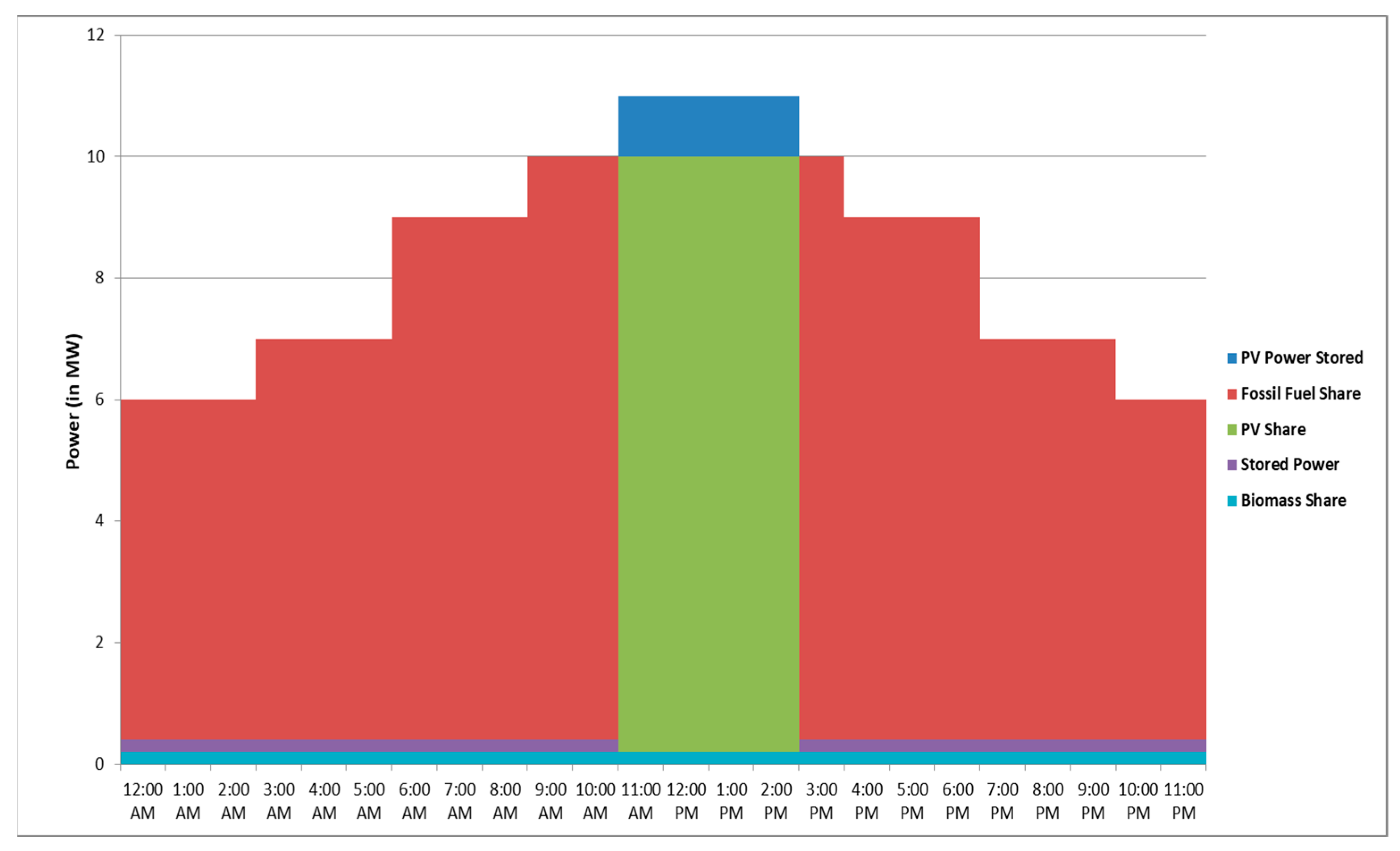
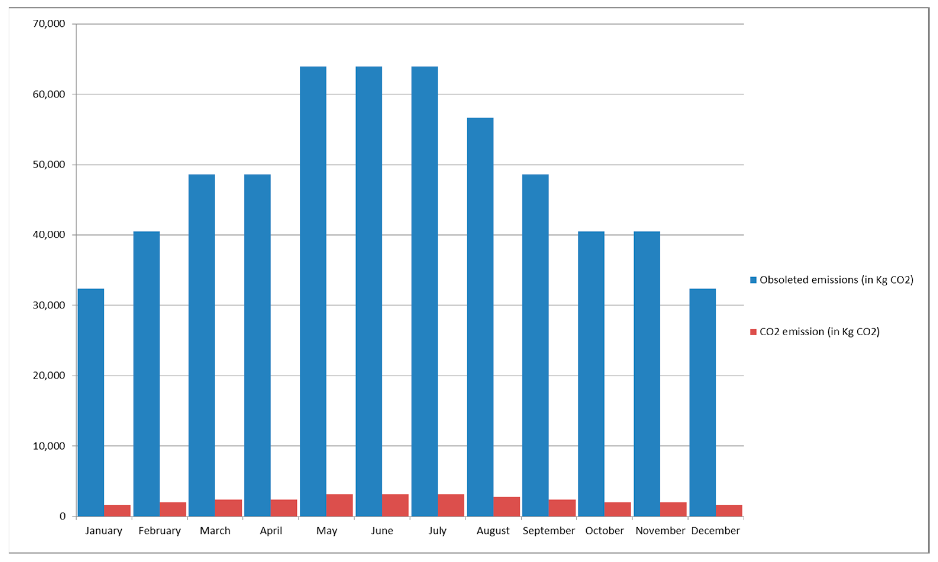
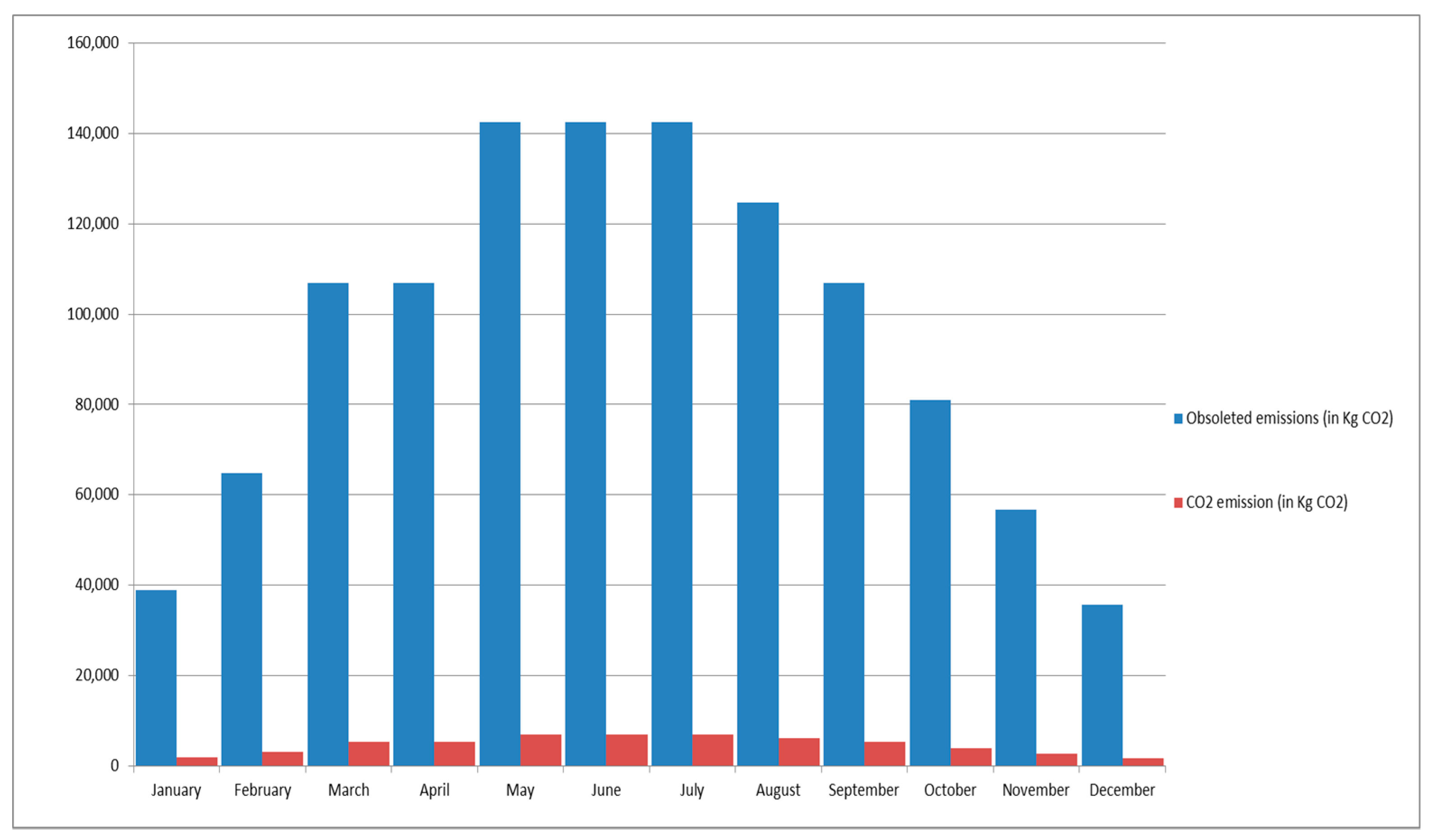
Scheduling of PV and biomass electrical energy generation to partially replace the conventional fossil fuel sources in a green energy seaport, is studied in this project. As carbon dioxide emissions affects the greenhouse gas and global warming phenomena, the impact of the environmentally friendly electrical energy generation unit on the reduction of carbon dioxide emissions and saving the environment is the main target of this research. Renewable sustainable electrical power sources are annually scheduled to be adapted with the available generation inputs. The study is based on two main strategies, which are eco-availability mode and Intelligent Scheduling (IS) mode. The Intelligent Reconfigured Whale Optimization Technique based Scheduling (IRWOTS) mode is executed for two scenarios. The first scenario is considering the system without battery storage units, to avoid the storage techniques’ problems of the excess generated power, while the storage units are considered in the second scenario.

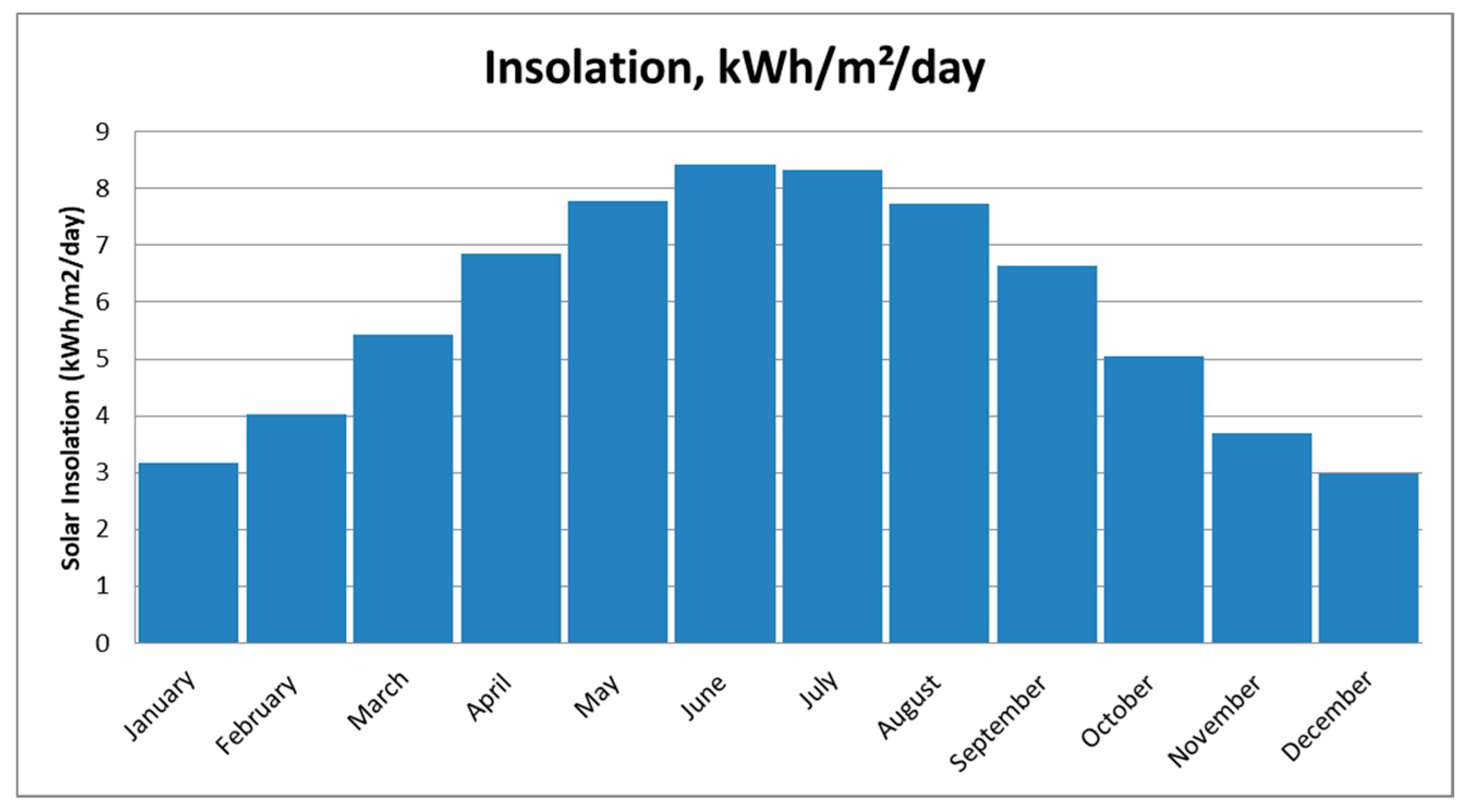
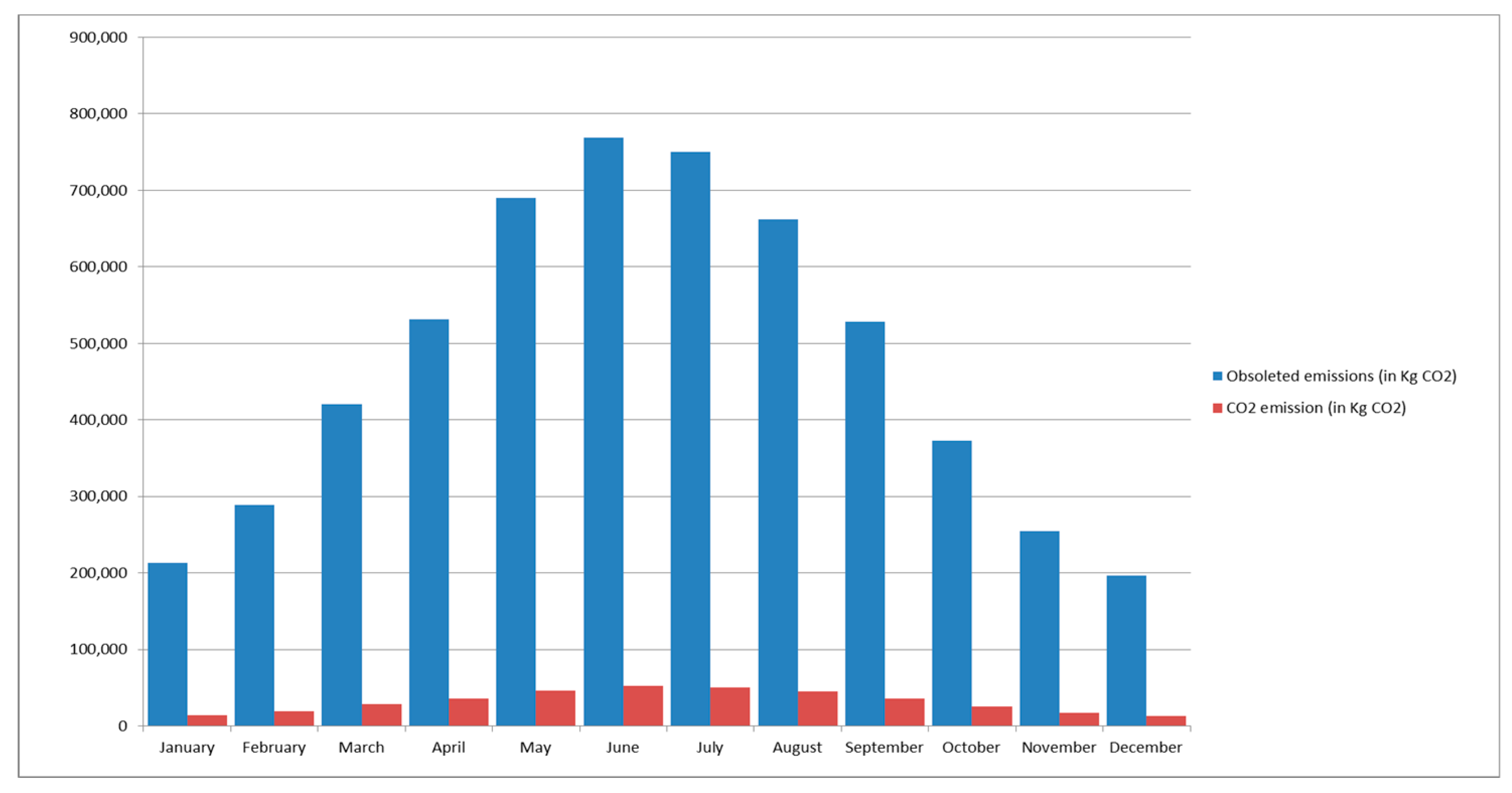
Photovoltaic generation depends on the average efficient daylight and solar insolation, which vary monthly and from one season to another. Regarding biomass electrical generation, it is suggested that total organic waste capacity of the community will be utilized in generating electrical power. The biomass generation is almost constant over the whole year. Sustainable efficient green energy port pattern is addressed by applying the combination of photovoltaic and biomass electrical power to Damietta port. It is also proposed that the extra generated green electrical energy be sold to the Egyptian Unified Electrical Power Network and the neighboring loads. The generation scheduling of biomass and photovoltaic electrical energy combination is assumed to vary from 40.2 MWh/day (in December—IRWOTS strategy-without battery storage unit) to 966 MWh/day (in June—Eco-availability strategy). The daily carbon dioxide emission oscillates between 1840 kg CO₂ and 52,163 kg CO₂. It results in clear daily carbon dioxide emission reduction that fluctuates between 36,240 kg CO₂ and 773,077.6 kg CO₂. The rate of obsoleted carbon oxides emission encourages the global societies to follow up the proposed model for the environment sake.

References

1. U.S. Department of Energy. Environment Baseline. Volume 1: Greenhouse Gas Emissions from the U.S. Power Sector. Office of Energy Policy and System Analysis, June 2016. Available online: https://energy.gov/sites/prod/files/2017/01/f34/Environment%20Baseline%20Vol.%201Greenhouse%20Gas%20Emissions%20from%20the%20U.S.%20Power%20Sector.pdf (accessed on 10 July 2017).
2. National Renewable Energy Laboratory (NREL). Life Cycle Greenhouse Gas Emissions from Electricity Generation. Available online: https://www.nrel.gov/docs/fy13osti/57187.pdf (accessed on 5 July 2017).
3. Sathaye, J.; Lucon, O.; Rahman, A.; Christensen, J.; Denton, F.; Fujino, J.; Heath, G.; Kadner, S.; Mirza, M.; Rudnick, H.; et al. Renewable energy in the context of sustainable development. In IPCC Special Report on Renewable Energy Sources and Climate Change Mitigation; Edenhofer, O., Pichs-Madruga, R., Sokona, Y., Seyboth, K., Matschoss, P., Kadner, S., Zwickel, T., Eickemeier, P., Hansen, G., Schlömer, S., Eds.; Cambridge University Press: Cambridge, UK, 2011; Available online: http://www.ipcc-wg3.de/report/IPCC_SRREN_Ch09.pdf (accessed on 5 August 2017).
4. Michael, J.J.; Selvarasan, I. Economic analysis and environmental impact of flat plate roof mounted solar energy systems. Sol. Energy 2017, 142, 159–170. [Google Scholar] [CrossRef]
5. Balbaa, A.; El-Amary, N.H. Green energy seaport suggestion for sustainable development in Damietta Port, Egypt. WIT Trans. Ecol. Environ. 2017, 214, 67–77. [Google Scholar]
6. Evans, A.; Strezov, V.; Evans, T.J. Sustainability considerations for electricity generation from biomass. Renew. Sustain. Energy Rev. 2010, 14, 1419–1427. [Google Scholar] [CrossRef]
7. Frankfurt School Team. Global Trends in Renewable Energy Investment 2016. Frankfurt School, FS-UNEP Collaborating Centre for Climate & Sustainable Energy Finance, 2016. Available online: http://fs-unep-centre.org/sites/default/files/publications/globaltrendsinrenewableenergyinvestment2016lowres_0.pdf (accessed on 20 March 2017).
8. Behl, R.K.; Chhibar, R.N.; Jain, S.; Bahl, V.P.; El Bassam, N. Renewable energy sources and their applications. In Proceedings of the International Conference on Renewable Energy for Institutes and Communities in Urban and Rural Settings, Agro House, India, 27–29 April 2012; Available online: https://www.surrey.ac.uk/ces/files/pdf/0700_WP_Renewable_ Energy_Sources.pdf (accessed on 20 March 2017).
9. Jackson, T. Renewable Energy Sources; Centre for Environmental Strategy, University of Surrey: Guildford, UK, 2000; Available online: https://www.surrey.ac.uk/ces/files/pdf/0700_WP_Renewable_Energy_ Sources.pdf (accessed on 20 March 2017).
10. History of Biomass. Available online: http://biomass-energy-project.weebly.com/history.html (accessed on 13 December 2016).
11. Biomass Energy. Available online: http://cr.middlebury.edu/es/altenergylife/sbiomass.htm (accessed on 13 December 2016).
12. Brower, M. Cool Energy: The Renewable Solution to Global Warming; Union of Concerned Scientists: Cambridge, MA, USA, 1990. [Google Scholar]
13. Howes, R.; Fainberg, A. The Energy Sourcebook: A Guide to Technology, Resources, and Policy; American Institute of Physics: College Park, MD, USA, 1991. [Google Scholar]
14. Schipfera, F.; Kranzla, L.; Leclèreb, D.; Sylvainb, L.; Forsellb, N.; Valinb, H. Advanced biomaterials scenarios for the EU28 up to 2050 and their respective biomass demand. Biomass Bioenergy 2017, 96, 19–27. [Google Scholar] [CrossRef]
15. Gavrilescu, D. Energy from biomass in pulp and paper mills. Environ. Eng. Manag. J. 2008, 7, 537–546. [Google Scholar]
16. Ruiza, J.A.; Juárezb, M.C.; Moralesb, M.P.; Muñozb, P.; Mendívilb, M.A. Biomass gasification for electricity generation: Review of current technology barriers. Renew. Sustain. Energy Rev. 2013, 18, 174–183. [Google Scholar] [CrossRef]
17. Puigjaner, L.; Pérez-Fortes, M.; Laínez-Aguirre, J.M. Towards a carbon-neutral energy sector: Opportunities and challenges of coordinated bioenergy supply chains-A PSE approach. Energies 2015, 8, 5613–5660. [Google Scholar] [CrossRef] [Green Version]
18. Tchapda, A.; Pisupati, S.V. A review of thermal co-conversion of coal and biomass/waste. Energies 2014, 7, 1098–1148. [Google Scholar] [CrossRef]
19. Molino, A.; Iovane, P.; Donatelli, A.; Braccio, G.; Chianese, S.; Musmarra, D. Steam gasification of refuse-derived fuel in a rotary kiln pilot plant: Experimental tests. Chem. Eng. Trans. 2013, 32, 337–342. [Google Scholar]
20. Chianese, S.; Fail, S.; Binder, M.; Rauch, R.; Hofbauer, H.; Molino, A.; Blasi, A.; Musmarra, D. Experimental investigations of hydrogen production from CO catalytic conversion of tar rich syngas by biomass gasification. Catal. Today 2016, 277, 182–191. [Google Scholar] [CrossRef]
21. Chianese, S.; Loipersböck, J.; Malits, M.; Rauch, R.; Hofbauer, H.; Molino, A.; Musmarra, D. Hydrogen from the high temperature water gas shift reaction with an industrial Fe/Cr catalyst using biomass gasification tar rich synthesis gas. Fuel Process. Technol. 2015, 132, 39–48. [Google Scholar] [CrossRef]
22. Florida Solar Energy Center. Available online: http://www.fsec.ucf.edu/en/ (accessed on 10 December 2016).
23. Psomopoulos, C.S.; Ioannidis, G.C.; Kaminaris, S.D. Electricity production from small-scale photovoltaics in urban areas. In Renewable and Alternative Energy: Concepts, Methodologies, Tools, and Applications; Information Resources Management Association: Hershey, PA, USA, 2017; Volume 3, Chapter 18; pp. 618–656. [Google Scholar] [CrossRef]
24. Psomopoulos, C.S. Solar energy: Harvesting the sun’s energy for sustainable future. In Handbook of Sustainable Engineering; Kauffman, J., Lee, K.-M., Eds.; Springer Science and Business Media: Dordrecht, The Netherlands, 2013; Chapter 56; ISBN 978-1-4020-8939-8. [Google Scholar] [CrossRef]
25. Green, M.A. Solar Cells: Operating Principles, Technology, and System Applications; Prentice-Hall, Inc.: Englewood Cliffs, NJ, USA, 1982. [Google Scholar]
26. Graziano, M.; Gillingham, K. Spatial patterns of solar photovoltaic system adoption: The influence of neighbors and the built environment. J. Econ. Geogr. 2014, 15, 815–839. [Google Scholar] [CrossRef]
27. Psomopoulos, C.S.; Ioannidis, G.C.; Kaminaris, S.D.; Mardikiset, K.D.; Katsikas, N.G. A comparative evaluation of photovoltaic electricity production assessment software (PVGIS, PVWatts and RETScreen). Environ. Process. 2015, 2 (Suppl. S1), 175–189. [Google Scholar] [CrossRef]
28. Batarlienė, N.; Jarašūnienė, A. Development of Advanced Technologies (AT) in green transport corridors. In Proceedings of the 9th International Scientific Conference Transbaltica, Vilnius, Lithuania, 7–8 May 2015; Volume 134, pp. 481–489. [Google Scholar]
29. Beleya, P.; Raman, G.; Chelliah, M.K.; Nodeson, S. Sustainability and green practices at Malaysian seaports: Contributors to the core competitiveness. J. Bus. Manag. Econom. 2015, 3, 23–27. [Google Scholar]
30. Anastasopoulos, D.; Kolios, S.; Stylios, C. How will Greek ports become green ports? Geo-Eco-Marina 2011, 17, 73–80. [Google Scholar]
31. Chao-Feng, S.; Mei-Ting, J.; Jing-Lei, Y.; Cui-Juan, H.; Chun-Li, C. The strategies and proposals for ecological port construction in China. J. US-China Public Adm. 2009, 6, 23–33. [Google Scholar]
32. Maritime Transport Sector (MTS). Available online: http://www.mts.gov.eg/en/ (accessed on 14 February 2017).
33. Kadiyala, A.; Kommalapati, R.; Huque, Z. Evaluation of the life cycle greenhouse gas emissions from different biomass feedstock electricity generation systems. Sustainability 2016, 8, 1181. [Google Scholar] [CrossRef]
34. Praxair Technology. Safety Precautions for Carbon Dioxide; Technical Communications; Praxair. Inc.: Tonawanda, NY, USA, 2009. Available online: http://catalogs.praxairdirect.com/i/27114-safety-precautions-for-carbon-dioxide/16 (accessed on 20 June 2017).
35. American Society of Heating. Refrigerating, and Air-Conditioning Engineers (ASHRAE) Standards. Available online: https://ashrae.iwrapper.com/ViewOnline/Standard_62.1-2016 (accessed on 8 March 2017).
36. Occupational Safety and Health Administration (OSHA). Available online: https://www.osha.gov/ (accessed on 8 March 2017).
37. Shindell, D.T.; Shindell, D.T.; Faluvegi, G.; Stevenson, D.S.; Krol, M.C.; Emmons, L.K.; Lamarque, J.F.; Pétron, G.; Dentener, F.J.; Ellingsen, K.; et al. Multimodel simulations of carbon monoxide: Comparison with observations and projected near-future changes. J. Geophys. Res. 2006, 111. [Google Scholar] [CrossRef] [Green Version]
38. Transportation Research Board and National Research Council. The Ongoing Challenge of Managing Carbon Monoxide Pollution in Fairbanks; The National Academies Press: Washington, DC, USA, 2002; Available online: https://www.nap.edu/catalog/10378/the-ongoing-challenge-of-managing-carbon-monoxide-pollution-in-fairbanks-alaska (accessed on 19 May 2017).
39. European Climate Foundation Report. Biomass for Heat and Power—Opportunity and Economics; European Climate Foundation: The Hague, The Netherlands, 2010. [Google Scholar]
40. Mateescu, C. Biomass to Biogas in rural regions. In Proceedings of the Sustainable Energy Best Practice in European Regions, Wales, UK, 13–15 March 2012. [Google Scholar]
41. European Biomass Association. BASIS—Biomass Availability and Sustainability Information System, Version #2; Report on Conversion Efficiency of Biomass; Supported by: Co-funded by the Intelligent Energy Europe, Programme of the European Union; European Biomass Association: Brussels, Belgium, 2015. [Google Scholar]
42. BIOS Company. Available online: http://www.bios-bioenergy.at/en/electricity-from-biomass/steam-turbine.html (accessed on 12 February 2017).
43. Hannula, I.; Kurkela, E. Liquid Transportation Fuels via Large-Scale Fluidised-Bed Gasification of Lignocellulosic Biomass; VTT Technology 91; VTT Technical Research Centre of Finland: Espoo, Finland, 2013. [Google Scholar]
44. Isaksson, J. Biomass Gasification-Based Biorefineries in Pulp and Paper Mills—Greenhouse Gas Emission Implications and Economic Performance. Ph.D. Thesis, Industrial Energy Systems and Technologies, Department of Energy and Environment, Chalmers University of Technology, Göteborg, Sweden, 2015. [Google Scholar]
45. Axelsson, E.; Pettersson, K. Energy Price and Carbon Balances Scenarios Tool (ENPAC)—A Summary of Recent Updates; Chalmers University of Technology: Göteborg, Sweden, 2014. [Google Scholar]
46. Axelsson, E.; Harvey, S. Scenarios for Assessing Profitability and Carbon Balances of Energy Investments in Industry; AGS Pathways Report 2010:EU1; The Alliance for Global Sustainability: Gothenburg, Sweden, 2010. [Google Scholar]
47. Mazzeo, D.; Matera, N.; Bevilacqua, P.; Arcuri, N. Energy and economic analysis of solar photovoltaic plants located at the University of Calabria. Int. J. Heat Technol. 2015, 33, 41–50. [Google Scholar] [CrossRef]
48. Shaltout, M.A. Egyptian Solar Radiation Atlas; New and Renewable Energy Authority (Egypt): Cairo Governorate, Egypt, 1991.
49. Salem, M.G. Solar Desalination as an Adaptation Tool for Climate Change Impacts on the Water Resources of Egypt; Technical Report; United Nations Educational, Scientific and Cultural Organization: Paris, France, 2013. [Google Scholar]
50. Siegel, M.M.D.; Klein, S.A.; Beckman, W.A. A simplified method for estimating the monthly-average performance of photovoltaic systems. Sol. Energy 1981, 26, 413–418. [Google Scholar] [CrossRef]
51. Mirjalili, S.; Lewis, A. The Whale Optimization Algorithm. Adv. Eng. Softw. 2016, 95, 51–67. [Google Scholar] [CrossRef]
52. Hu, H.; Bai, Y.; Xu, T. A whale optimization algorithm with inertia weight. WSEAS Trans. Comput. 2016, 15, 319–326. [Google Scholar]
53. Aljarah, I.; Faris, H.; Mirjalili, S. Optimizing connection weights in neural networks using the whale optimization algorithm. Soft Comput. 2018, 22, 1–15. [Google Scholar] [CrossRef]
54. Kaveh, A.; Ghazaan, M.I. Enhanced whale optimization algorithm for sizing optimization of skeletal structures. Mech. Based Des. Struct. Mach. 2017, 45, 345–362. [Google Scholar] [CrossRef]
55. Prasad, D.; Mukherjee, A.; Shankar, G.; Mukherjee, V. Application of chaotic whale optimisation algorithm for transient stability constrained optimal power flow. IET Sci. Meas. Technol. 2017, 11, 1002–1013. [Google Scholar] [CrossRef]
56. Mafarja, M.M.; Mirjalili, S. Hybrid Whale Optimization Algorithm with simulated annealing for feature selection. Neurocomputing 2017, 260, 302–312. [Google Scholar] [CrossRef]
57. Abd El Aziz, M.; Ewees, A.A.; Hassanien, A.E. Whale Optimization Algorithm and Moth-Flame Optimization for multilevel thresholding image segmentation. Expert Syst. Appl. 2017, 83, 242–256. [Google Scholar] [CrossRef]
58. Dinakara Prasad Reddy, P.; Veera Reddy, V.C.; Gowri Manohar, T. Optimal renewable resources placement in distribution networks by combined power loss index and whale optimization algorithms. J. Electr. Syst. Inf. Technol. 2017, 28, 669–678. [Google Scholar]
59. Ling, Y.; Zhou, Y.; Luo, Q. Lévy Flight Trajectory-Based Whale Optimization Algorithm for Global Optimization. IEEE Access 2017, 5, 6168–6186. [Google Scholar] [CrossRef]
60. World Port Source, Port of Damietta? Available online: http://www.worldportsource.com/ports/review/EGY_Port_of_Damietta_670.php (accessed on 14 June 2017).
61. Damietta Port Authority. Available online: http://www.dpa.gov.eg/ (accessed on 16 July 2017).
62. Damietta Port. Available online: http://www.imsalex.com/damietta.html#q1 (accessed on 16 July 2017).
63. Alexandria Chamber of Shipping, Damietta Port. Available online: http://www.acs.org.eg/port-type/damietta-port/ (accessed on 16 July 2017).
64. Weather-Forecast.com, Damietta Weather Forecast. Available online: http://www.weather-forecast.com/locations/Damietta (accessed on 16 July 2017).
65. Cargo Supervision and Surveying Office. Available online: http://www.cargo-sup-sur.com/Domiate%20Map.html (accessed on 16 July 2017).
66. Weatherbase, Damietta, Egypt. Available online: http://www.weatherbase.com/weather/weatherall.php3?s=601777&cityname=Damietta%2C+Dumyat%2C+Egypt&units= (accessed on 10 June 2017).
67. GAISMA, Damietta, Egypt. Available online: http://www.gaisma.com/en/location/damietta.html (accessed on 10 June 2017).
68. Open Power System Data. Available online: https://open-power-system-data.org/ (accessed on 3 December 2017).
69. Breeze, P. The Cost of Power Generation: The Current and Future Competitiveness of Renewable and Traditional Technologies; Business Insights Ltd.: London, UK, 2010; Available online: http://lab.fs.uni-lj.si/kes/erasmus/The%20Cost%20of%20Power%20Generation.pdf (accessed on 3 December 2017).
70. International Renewable Energy Agency. Renewable Power Generation Costs in 2017; IRENA: Abu Dhabi, UAE, 2018; Available online: http://irena.org/-/media/Files/IRENA/Agency/Publication/2018/Jan/IRENA_2017_Power_Costs_2018.pdf (accessed on 4 December 2017).
71. Luckow, P.; Stanton, E.A.; Fields, S.; Ong, W.; Biewald, B.; Jackson, S.; Fisher, J. Spring 2016 National Carbon Dioxide Price Forecast; Synapse Energy Economics, Inc.: Cambridge, MA, USA, 2016; Available online: http://www.synapse-energy.com/sites/default/files/2016-Synapse-CO2-Price-Forecast-66-008.pdf (accessed on 10 December 2017).
72. The World Bank. Available online: http://www.worldbank.org/en/programs/pricing-carbon (accessed on 13 December 2017).
73. Markets Insider. Available online: http://markets.businessinsider.com/commodities/co2-emissionsrechte (accessed on 13 December 2017).
Figure 1. Solar energy intensity in Egypt [48].
Energies 11 00535 g001
Figure 2. Bubble-net hunting behaviour of humpback whales [51,52,53,54].
Energies 11 00535 g002
Figure 3. Bubble-net search shrinking encircling model of humpback whales [51,52,53,54].
Energies 11 00535 g003
Figure 4. Model of Bubble-net search spiral position updating model [51,52,53,54].
Energies 11 00535 g004
Figure 5. Reconfigured Whale Optimization Technique (RWOT) flowchart.
Energies 11 00535 g005
Figure 6. The renewable electrical energy generation scheduling strategies block diagram.
Energies 11 00535 g006
Figure 7. Different electrical power sources that feed the Damietta seaport (the grid and suggested renewable energy sources).
Energies 11 00535 g007
Figure 8. Damietta port typical daily electrical power consumption pattern (power consumption chronological curve).
Energies 11 00535 g008
Figure 9. Average solar insolation (in kWh/m2/day) versus the months of the year.
Energies 11 00535 g009
Figure 10. The average PV CO2 emission compared to the obsoleted CO2 emission based on Eco-availabiltiy strategy.
Energies 11 00535 g010
Figure 11. Typical daily electrical power generation scheduling and sharing pattern according to Eco-availability strategy.
Energies 11 00535 g011
Figure 12. Electrical power generation scheduling and sharing pattern according to IROWTS strategy (without battery storage unit) for a typical day in December.
Energies 11 00535 g012
Figure 13. Electrical power generation scheduling and sharing pattern according to IROWTS strategy (without battery storage unit) for a typical day in June.
Energies 11 00535 g013
Figure 14. Electrical power generation scheduling and sharing pattern according to IROWTS strategy (with battery storage unit) for a typical day in December.
Energies 11 00535 g014
Figure 15. Electrical power generation scheduling and sharing pattern according to IROWTS strategy (with battery storage unit) for a typical day in June.
Energies 11 00535 g015
Figure 16. The average PV CO2 emission compared to the obsoleted CO2 emission based on IRWOTS strategy (without battery storage unit).
Energies 11 00535 g016
Figure 17. The average PV CO2 emission compared to the obsoleted CO2 emission based on IRWOTS strategy (with battery storage unit).
Energies 11 00535 g017