Line-to-Line Fault Analysis and Location in a VSC-Based Low-Voltage DC Distribution Network


The Key Laboratory of Smart Grid of Ministry of Education, Tianjin University, Tianjin 300072, China
*
Author to whom correspondence should be addressed.
Energies 2018, 11(3), 536; https://doi.org/10.3390/en11030536
Submission received: 24 January 2018
/
Revised: 23 February 2018
/
Accepted: 26 February 2018
/
Published: 2 March 2018
(This article belongs to the Special Issue Emerging Power Electronics Technologies for Power Systems and Machine Drives)
Abstract
:A DC cable short-circuit fault is the most severe fault type that occurs in DC distribution networks, having a negative impact on transmission equipment and the stability of system operation. When a short-circuit fault occurs in a DC distribution network based on a voltage source converter (VSC), an in-depth analysis and characterization of the fault is of great significance to establish relay protection, devise fault current limiters and realize fault location. However, research on short-circuit faults in VSC-based low-voltage DC (LVDC) systems, which are greatly different from high-voltage DC (HVDC) systems, is currently stagnant. The existing research in this area is not conclusive, with further study required to explain findings in HVDC systems that do not fit with simulated results or lack thorough theoretical analyses. In this paper, faults are divided into transient- and steady-state faults, and detailed formulas are provided. A more thorough and practical theoretical analysis with fewer errors can be used to develop protection schemes and short-circuit fault locations based on transient- and steady-state analytic formulas. Compared to the classical methods, the fault analyses in this paper provide more accurate computed results of fault current. Thus, the fault location method can rapidly evaluate the distance between the fault and converter. The analyses of error increase and an improved handshaking method coordinating with the proposed location method are presented.
1. Introduction
In recent years, distributed generation has been promoted on a large scale, primarily for DC current systems. For this reason, hybrid AC/DC power systems have developed considerably. Voltage source converters (VSCs) attracted widespread attention because of their excellent control and operation characteristics in low-voltage DC distribution networks [1,2]. Hence, technology to protect VSC-based DC distribution networks has become a heavily researched topic. However, the relevant research is limited, especially in the area of fault analysis and location. Some papers have been published in the last two years, with the relevant results summarized below.
For DC relay protection, Baran et al. [3] proposed a protection method based on early overcurrent. Yang et al. [4] considered that freewheel diodes were very easy to damage because of the severe overcurrent resulting from a capacitance discharge. Next, Baran et al. [3] proposed replacing the diodes with emitter turn-off devices (ETOs) to provide diodes with the capacity to block the current. Moreover, Baran et al. [3] adopted an ETO-based capacitance DC circuit breaker to cut off the capacitance branches and block the discharge current. However, this method increased the power loss to some extent. Deng et al. [5] developed an expression establishing the relationship between the peak value of the discharge current and the current-limiting inductance with the result that a simple inductance was effectively used to protect the diodes. Several papers have investigated the superconducting fault current limiter [6,7,8,9].
As the theoretical basis for fault location and current-limiting technology, papers examining short-circuit faults or ground fault analyses in VSC-based DC networks are still inadequate. Most of these papers’ results are based on numerical simulation tests, lacking theoretical analysis. These studies’ conclusions are made based on qualitative relationships or curves derived from simulated data. Yang et al. [4] first divided the fault into 3 stages ((a) capacitor discharge, (b) diodes freewheel and (c) grid current feeding) and provided in-depth theoretical analyses of the transient discharge process in a 2nd-order circuit model, eventually proposing formulas for fault current and voltage. Deng et al. [5] performed similar work to determine the relationship between the transient fault current and parameters of capacitance and inductance, providing a theoretical basis for current limiting by inductance on the DC side. Consequently, almost all later theories, both in high-voltage DC (HVDC) and low-voltage DC (LVDC) systems, regarding fault analyses were developed based on the above results, which may mislead the current limiter designs and fault location principles to some extent. Furthermore, few papers present research on steady-state fault analysis. A whole fault process includes both a transient-state fault and a steady-state fault. Steady-state fault analysis is of great significance for efforts to limit current.
However, almost all study about fault analyses are based on an HVDC-VSC transmission system [4,5,10,11,12,13,14,15], which presents several problems in a LVDC distribution network. The main problem is that stage 1, capacitor discharge, does not arise in a 2nd-order circuit model because the DC voltage is not considerably higher than that of the AC side. Under this circumstance, the diodes freewheel throughout the whole fault process, and the fault is better represented by a 3rd-order circuit model. Thus, the theoretical formulas in [4] have omitted the forced response and resulted in larger errors in fault current computing or location of an LVDC system. Alwash et al. [16] initially considers the diodes conduction stage and the current feeding from AC side in fault analyses. However, it omits the capacitance branch which is unsuitable for some fault cases.
In the study of fault locations, a prevalent method is injecting signals into a faulty cable with a probe power unit (PPU) [17,18]; a handshaking method is proposed in [19] to locate a fault without any communication models. These methods must disconnect all the sources from the system, which greatly reduces the speed of power recovery. In addition, the handshaking method may lose selectivity in some cases. Yang et al. [20] determined the fault distance by analyzing the fault information sampled by two mutual inductances separated by a known distance, but the expense of measuring the equipment is double. Tang et al. [21] located the fault by comparing the derivative, time interval or oscillation mode of the fault current in different places. It is a communication-based method which is unfit for a distribution network. Other studies have attempted to develop an accurate fault location technology, with research still focusing on the method based on a traveling wave [22,23,24,25]. However, the traveling wave location method is difficult to adopt in a distribution network with short cables because the demanded sampling frequency is too high. Additionally, some papers, such as [4,26], previously referred to the fault analysis results and determined the fault distance by solving for the parameters of resistance and inductance. However, the method in [26] has lower accuracy than that in [4] with fault resistance because its fault distance is calculated from measured resistance and unit resistance of a cable (R/km).
However, because the fault stages differ from the HVDC system, the theoretical formulas in [4] are not appropriated for fault location in the LVDC distribution system. In addition, steady-state fault analysis is indispensable because the DC-linked capacitors are cut in some protection scheme [3]. However, relevant works are deficient.
Thus, in accordance with the low-voltage distribution network itself, this paper compares the whole fault process in the HVDC transmission and LVDC distribution systems, giving a reasonable explanation for their differences. Then, we divide short-circuit fault into two stages: the transient- and steady-state stages. The primary focus of the paper is fault analysis during the steady-state stage. Next, a 3rd-order circuit was adopted for transient-state short-circuit fault analyses to correct the shortcomings of the 2nd-order circuit model analysis results in a low-voltage network. A fault location method adopting both transient and steady fault components was proposed based on the theoretical analyses. The computed results of fault current base on theoretical formulas in [4] and this paper are compared to verify the improvement in the computed accuracy. In addition, the reasons for the increase in errors in high fault resistance short-circuit faults is explained in brief. Finally, an improved location method is proposed by coordinating with the classical handshaking method, by which the performance of the handshaking method is enhanced.
This paper is organized as follows: Section 2 presents the comparison of fault processes, detailed fault analyses, and a theoretical solution for transient and steady-state short-circuit faults is developed. Specific parameters and simulations in PSCAD/EMTDC are provided in Section 3. The fault location method, data on the location results, error analysis and coordination with other methods are presented in Section 4.
2. LVDC Cable Short-Circuit Fault Analysis
2.1. Fault Stages Comparison
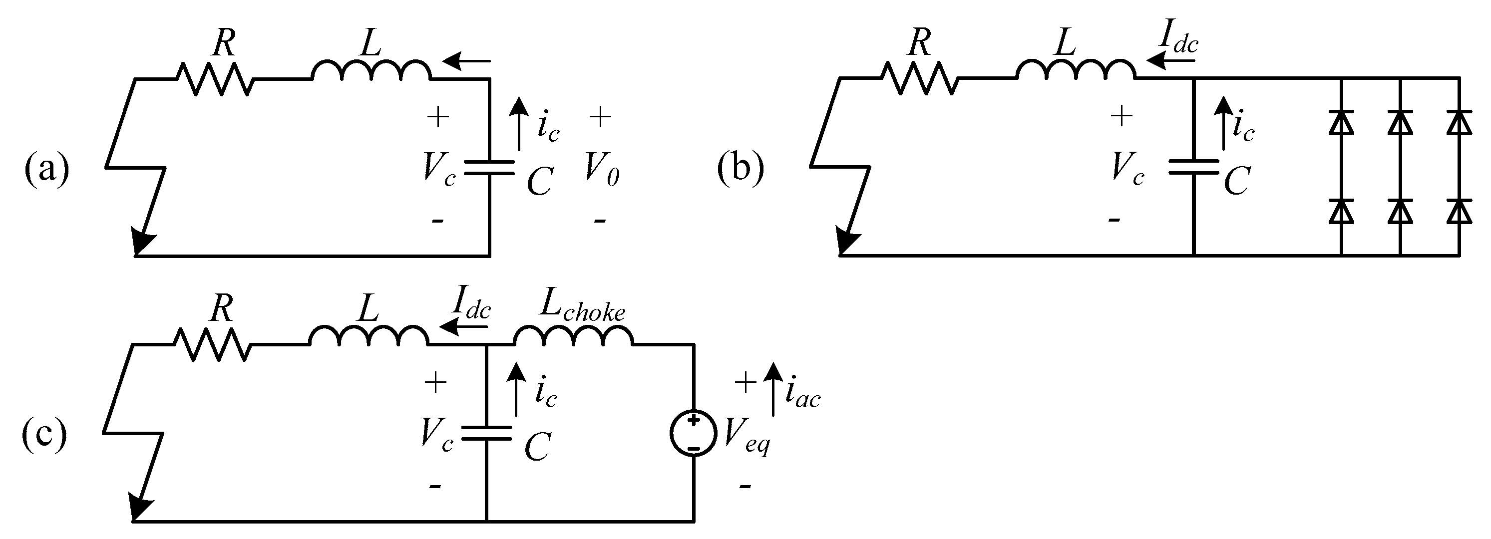
When a short-circuit fault occurs, all DC-linked capacitances in the system will discharge to the fault location. This discharge leads the system voltage to collapse and the fault current to surge. As the classical theory proposed in [4], a whole fault progresses in three stages: (i) Capacitor discharges stage (Natural Response); (ii) Diode freewheel stage (Natural Response under the circumstance of ); and (iii) Grid-side current feeding stage (Forced Response). The classical equivalent circuits and electrical waveforms of different stages are shown as Figure 1 and Figure 2a, respectively. The fact that stage 2 is the most challenging for freewheel diodes is generally accepted. However, stage 2 merely arise under the specified condition. Classically, the DC voltage will oscillate under the condition and drop to zero at , where is fault occurring moment, , and .
However, a fault progresses differently in the LVDC distribution system, and the main differences are reflected in stage 1. Note that the derivatives of grid-side current are as follows:
where is the difference in DC voltage and AC line voltage . In the HVDC transmission system, is much higher . This means that is high enough and that time is sufficient for the freewheel diodes to be blocked swiftly before gets lower than in stage 1. Just the natural response arises in a 2nd-order circuit in this stage (Figure 2a). In the LVDC distribution system, is not so high. This means that and are low; therefore, time is insufficient for the freewheel diodes to be blocked before gets lower than in stage 1. Once inequality is established, freewheel diodes will not be blocked. Both the natural and forced responses arise in a 3rd-order circuit in this stage (Figure 2b). Thus, considerable errors arise in fault current computation and fault location if analyzed results in [4] continue to be adopted. Moreover, the criterion for DC voltage oscillation and estimated time when voltage reaches zero in HVDC system is unsuitable for LVDC system as the whole forced response feeding from AC-side is omitted. Whether DC voltage oscillates and when it drops to zero are depend on the actual expression of transient-state fault current. Fault analysis in a 3rd-order circuit must be proposed.
In this paper, the fault process is divided into two stages: the transient- and the steady-state stages. According to the simulated results, the transient duration is generally approximately 2 ms, and the surge current is more than ten times the normal current. The steady-state develops as the DC-side power steadies. Until all breakers trip, this stage lasts approximately 100 ms [21]. The fault current is a steady DC current with 6 waves, where the amplitude is influenced by the AC-side resistance, inductance and DC-side resistance. The amplitude of the steady fault current is much lower than that of the surge current, but it has a long duration. Therefore, the freewheel diodes will be damaged without appropriate current-limiting measures.
Thus, the peak value of the surge current and the amplitude of the steady current are the most significant parameters in fault analyses.
2.2. Fault Stages Comparison
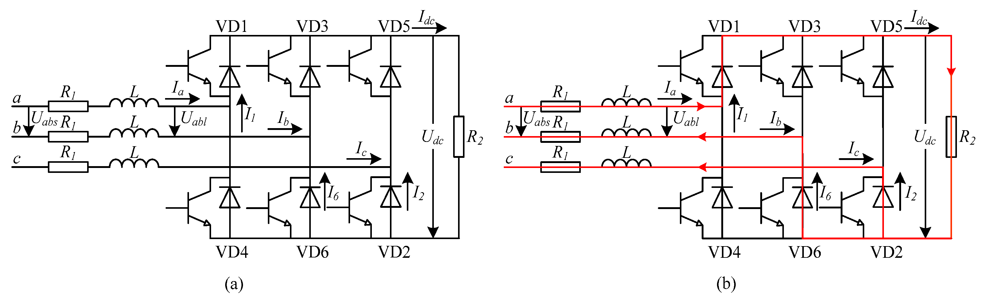
DC-linked capacitance and inductance have no influence on the amplitude of the steady fault current. Therefore, a simplified circuit model is adopted as depicted in Figure 3a. The actual waveforms of the model in Figure 3a are presented as Figure 4. R1, L and R2 are the total AC resistance, AC inductance and DC resistance, respectively.
During the steady-state process, all freewheel diodes conduct for half of a primitive period, which is different from the situation observed in a three-phase rectification circuit (freewheel diodes conduct for one third of a primitive period). This finding is attributable to the freewheel effect of the AC-side inductance when the AC voltage Uabc is lower than the DC voltage Udc. However, when the current of the AC-side inductance decreases to 0 (point A in Figure 4), the freewheel diodes prevent the current from decreasing further. Therefore, the rate of change in the current of the AC-side inductance di1/dt abruptly changes to 0, which results in Uabl = Uabs < Udc, with the result that diode 1 is blocking and diode 4 is conducting. Note that each diode conducts for less than half of a primitive period when .
A primitive period can be divided into 6 equivalent periods based on the conducting status of the freewheel diodes, where each period corresponds to three different conducting freewheel diodes. Because all periods are the same, any one period can be chosen for analysis. In this paper, period ③, in which diodes 1, 2 and 6 are conducting, is analyzed in detail. The current path and direction are shown in Figure 3b. Assume that the starting time of period ③ is 0 and the coordinate system is established as shown in Figure 4.
Because of the equivalence relations—, and —we obtain a 1-order differential equation after plugging the above relationships into Equations (2) + (3):
where . The solution of the above equation is
where
Note that and in the steady-state process. Thus, the amplitude of the steady-state voltage can be estimated as
In a similar way, the amplitude of the steady-state current can be estimated as
2.3. Transient-State Fault
The transient-state fault is more difficult to analyze than the steady-state fault. Based on the boost effect of the VSC, the voltage at the DC side is always higher than that of the AC side. Especially in the HVDC transmission system, the voltage of the DC side is much higher (like AC/DC is 0.392 kV/1.0 kV in [4]). Thus, all freewheel diodes will be blocked in stage 1 and each side will be isolated. Therefore, it is simple and reasonable to analyze this system in the 2nd-order circuit model. However, in the LVDC distribution system, the voltage of the DC side is not sufficiently high. As the analysis in Section 2.1, the fault should be analyzed using the 3rd-order circuit model.
In this paper, the transient-state fault process is divided into the natural response process and the forced response process. Compared to the transient fault current, the normal current is very small and can be omitted. To simplify the analysis, the DC-side circuit is regarded as open. Thus, the transient fault corresponding circuits are shown in Figure 5.
Figure 5a is the circuit representing the natural response process. and are the equivalent parameters of the AC-side components. Two of the three-phase branches are always in parallel connection, connected with the remaining branch in series (circuit structure in Figure 4a). Thus, consider and to be equal to and , respectively. and are the total parameters of the DC-side components. is the parameter of DC-linked capacitance. The DC-linked capacitance discharges to each branch at the voltage of the operating value, . Figure 5b depicts the circuit representing the forced response process. Considering that the DC source is connected to the circuit at the moment of fault occurrence, the magnitude of the source can be equal to the step signal, the amplitude of which is derived from the output voltage of three-phase full-wave bridge circuit .
(1) Forced response of the transient-state fault:
According to Equations (9)–(11), the state equations are
Applying Formula , the characteristic equation can be obtained as follows:
where
Thus, applying the radical formula for a cubic equation, a real root and dual conjugate complex roots can be obtained as follows:
Hence, the analytic expression of the forced response surge current in Figure 4a is
Under the initial conditions of , and . Note that . Thus, the constant terms , , , and the final analytical expression of the forced response surge current is
(2) Natural response of the transient-state fault:
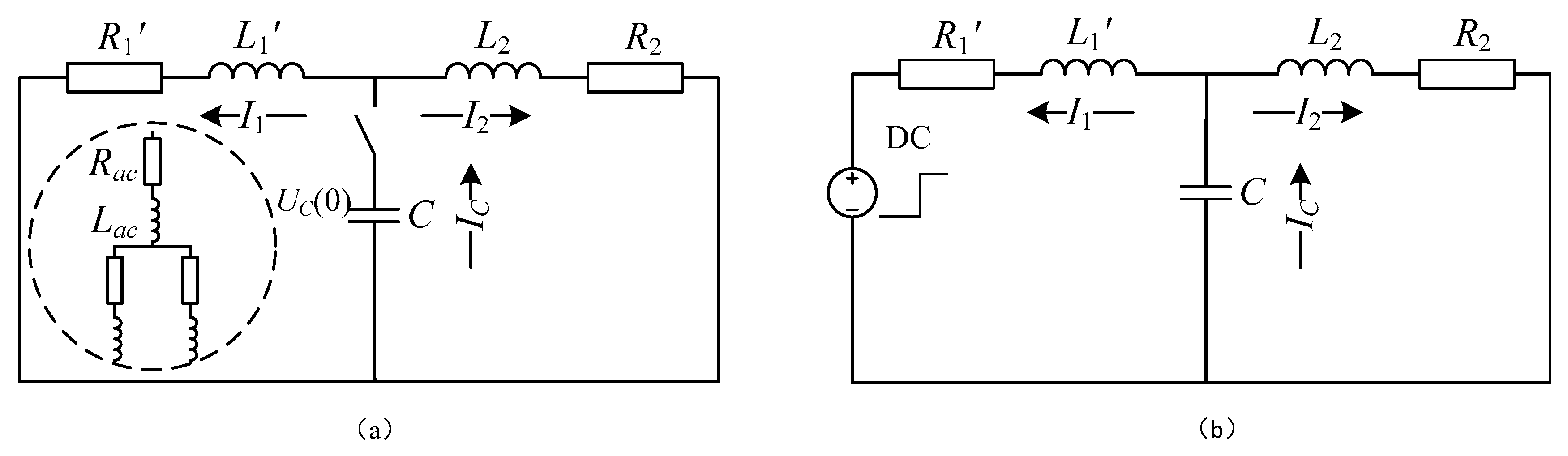
The DC-linked capacitance discharges to two resistance-inductance (R-L) branches in the natural response circuit. An equivalent branch is adopted to replace the two RL branches as shown in Figure 6. Hence, the RLC circuit shown in Figure 6 simplifies the analysis.
Assuming that and , the following equations can be obtained:
where
Hence, the inherent frequency, attenuation coefficient and natural oscillation frequency of the above RLC circuit are , and , respectively. Thus, the analytical expression of the natural response surge current in the capacitance branch is
The current content is inversely proportional to the impedance of each RL branch. Thus, the analytical expression of the natural response surge current in the DC branch is
Note that the above analytical results are reasonable under the circumstance of
and error increases considerably if Equation (23) is unsatisfied.
(3) Computation of the complete response and the surge current:
The analysis presented above shows that the complete response of the short-circuit fault surge current equals the sum of the forced response surge current and the natural response surge current in an equivalent linear circuit
Theoretically, applying Equation (24), the peak value of the surge current can be calculated. Because the derivative of the current equals 0 at the time of the peak, the peak time can be obtained by
Thus, the peak value of the current can be obtained as .
3. Case Studies
Simulations were completed in PSCAD/EMTDC 4.5 (Manitoba HVDC Research Centre, Manitoba, Canada). The parameters of the low-voltage distribution network are shown in Table 1. The RMS of the AC side line voltage and phase voltage . Therefore, the DC voltage source in the equivalent circuit . The cables adopt π-model parameters, and grounding capacitances are omitted.
Figure 7 shows the comparison between the theoretical waveform1 obtained by Equation (24), theoretical waveform2 obtained by formulas in [4] and the simulated waveform of the surge current, with a metal short-circuit fault occurring on 2 km of the whole cable. As the figure shows, nearly no errors are observed between the theoretical waveform1 and simulated waveform when the fault occurs with no resistance. However, considerable errors appear between the theoretical waveform2 and simulated waveform. The theoretical value is much lower than the simulated value, as the forced response from AC-side is omitted.
Table 2 shows the theoretical value, simulated value and the error when a metal short-circuit fault occurs over a different distance. Moreover, the theoretical value of the surge current includes a theoretical value obtained by Equation (24) (theoretical transient-state peak current1) and a theoretical value obtained by formulas in [4] (theoretical transient-state peak current2). As Table 2 shows, in the metal short-circuit fault case, current1 has little error, which is slightly higher than the simulated results. The simulated results demonstrate that the error is approximately 2%, and not more than 4%. Meanwhile, current2 is much lower than simulated results, and the error increases up to 15%. Note that the error increases with increasing fault distance. The error in the steady-state fault current decreases with increasing fault distance. The error is more than 5% within a fault distance of 3 km and less than 5% at a fault distance of 4 km or more. Moreover, the error of the steady-state fault current stabilized approximately 5%.
4. Fault Location and Protection Coordination
4.1. Short-Circuit Fault Location and Analysis
Because the location method based on stage 1 in [4] is inaccurate, this paper proposed a fault location method adopting the amplitude of the steady-state fault current and the transient-state surge peak current based on the fault analyses presented above.
Referring to the simulation result and Equation (8), the value of the resistance on the DC side can be obtained. Due to the 5% computational error, 1.05-fold of the steady-state fault current should be plugged into Equation (8). The DC-side resistance can be obtained as follows:
Based on the transient-state fault analysis, a function establishing a relationship among the DC-side resistance , DC-side inductance and transient-state surge peak current can be obtained as follows:
Obviously, can be obtained when and are given. Based on the linear relationship between and fault distance , a location result can be obtained.
The location results and errors of the proposed location method for different fault distances are shown in Table 3 at fault resistances of and . The error increases with increasing fault distance and resistance. The method has high accuracy with an error less than 5% in the metal short-circuit fault case.
However, the error increases significantly in the non-metal short-circuit case due to the following causes: (i) dissatisfying the circumstance Equation (23) or (ii) the impedance of the DC side is much higher than that of the AC side. This can be explained as follows:
Note that is mainly supplied by natural response current . According to Equation (22), can be approximatively expressed as follows:
where is regarded as constant.
Taking Equation (28)’s partial derivative respect to , the derivative function can be obtained as follows:
Equation (30) means that a small measured or computed error of will result in high deviation of under the circumstance of . Therefore, the fault distance determined by is inaccurate.
Moreover, according to Equation (30), the location error can be reduced by enlarging the value of . Thus, a limiter is installed at AC-side to reduce the error in Table 3. The limiter’s parameters are and . The location results and errors are shown in Table 4. Obviously, the location error declines dramatically with the limiter installed. In addition, reliable measurement, monitoring and sensor devices are required for error elimination.
4.2. Coordination with the Handshaking Method
As analyzed above, the location method proposed has a higher error in a remote fault condition with high resistance. Thus, it has limited advantage when adopted as an independent location method. However, the biggest advantage of this method is easy to realize. The faults are rapidly located without any control and with small quantities of computation. Hence, it is more suitable for fast fault estimation and coordinate with other locations.
In [19], Tang and Ooi proposed a handshaking method for a location fault without any communications in the multi-terminal loop-type DC system. In this method, faults are located according to the following principles:
- Disconnect all the sources;
- Open the switches that carry the fault current from the bus to the line;
- Reconnect all the sources; and
- Re-close the switches with both of their poles connected to an energized bus.
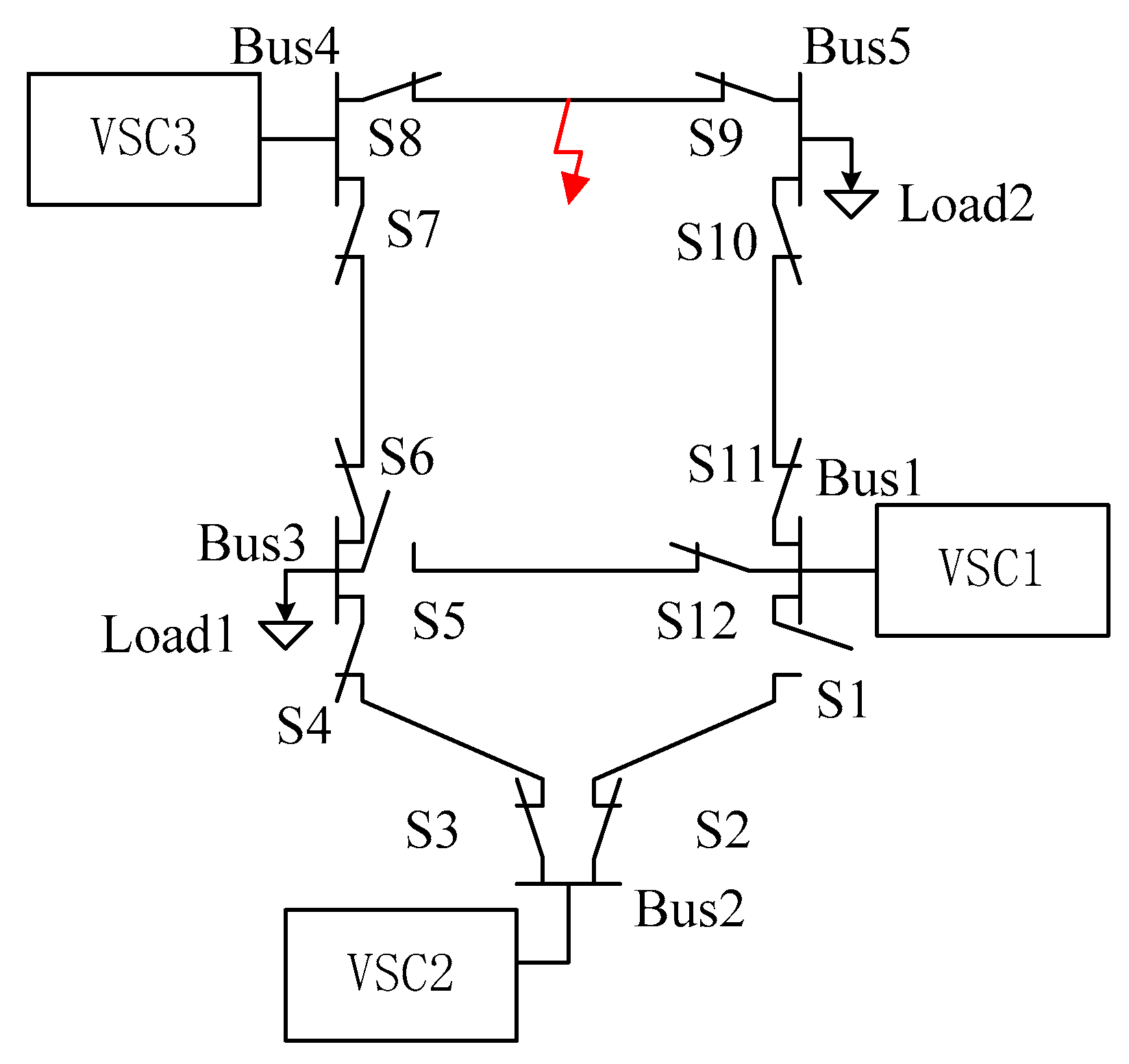
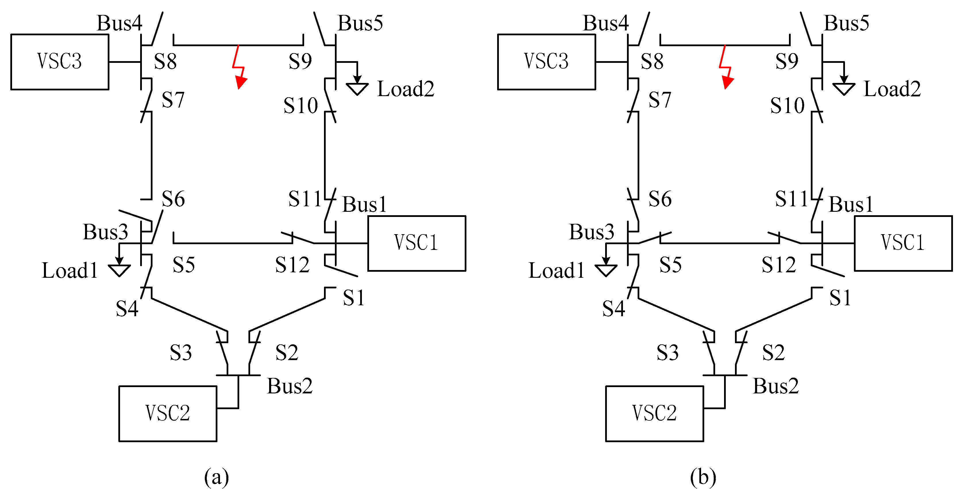
This method can effectively locate and isolate the fault extent. However, too many switch operation times and limited selectivity are its disadvantages. For instance, a multi-terminal loop-type DC distribution network is operating as Figure 8 shows. The system parameters are the same as those shown in Table 1, and the length of each cable is 1 km. To ensure safety, the system is open-loop so S1 and S5 are opened. If a fault occurs as Figure 8 shows, according to principle 2 above, S3, S6, S8, S9 and S11 will be opened (Figure 9a). However, according to principle 4 above, only S1 is re-closed after all the sources are reconnected (Figure 9b). Obviously, the fault is located and isolated, but the power supply of load1 and load2 are interrupted.
The handshaking method loses its selectivity because not all the buses are connected to a source. However, the location method proposed in Section 4.1 can be adopted to coordinate with the handshaking method to reduce switch operation times and ensure selectivity under this circumstance. The improved principles are as follows:
p1. Estimate the fault distance according to the current of each VSC branch;
p2. Determine if the operation instructions of switches connected to the same active bus with VSC should be blocked according to the estimated fault distance;
Then, the remaining switches operate as steps 1–4 of the original principles.
The criterion to block the switch operation instructions is , where is the minimal length of cables connected to active bus, and is the fault distance calculated by the method proposed in Section 4.1. For instance, the same fault occurs in the DC system, and the peak currents of VSC are , and , respectively. According to Equations (26) and (27), the distances of the fault to VSC1, VSC2 and VSC3 are 1.45 km, 2.01 km and 0.63 km, respectively (Data in detail are given in appendices). According to step p2, the operation instructions of switches connected to Bus1 and Bus2 should be blocked. Thus, S1, S2, S3, S11 and S12 will not be opened or re-closed until the last step. The remaining switches S6, S8 and S9 will be opened according to step 2 (Figure 10a), and only S6 will be reclosed according to step 4 (Figure 10b).
Hence, switch operation times are reduced and selectivity is ensured after the handshaking method is improved by coordinating with the fault distance estimation.
5. Conclusions
This paper identified the difference in fault analyses between the HVDC-VSC and LVDC-VSC systems. The steady-state fault analyses and the transient-state fault analyses considering forced response and adopting the 3rd-order circuit model are proposed. The new theories are in accordance with the line-to-line short-circuit fault characteristics in a LVDC distribution network based on a VSC. Simulation results demonstrate that the steady-state fault current and transient-state surge peak current can be computed through analytical expressions derived to describe the fault. Compared to the classical theories neglecting the forced response in [4], the analytical expressions in this paper have fewer errors and more significant implications for current limiter designs and fault locations. The proposed fault location method adopting steady-state and transient-state components is effective and meaningful in the case of line-to-line short-circuit faults. The reason for the increase in location error with increased fault distance and resistance is analyzed at the end of the paper, and the corresponding measure is proposed to improve the location accuracy effectively. For implementation in practice, the location method is adopted to coordinate with the handshaking method. Obviously, the improved method has decreased switch operation times and higher selectivity. Further research may lead to further method improvements to reduce location error.
Acknowledgments
This work was supported in part by the National Natural Science Foundation of China under Grant 51207103 and 51577129, by the Tianjin Municipal Natural Science Foundation under Grant 14JCYBJC21000 and by National High Technology Research and Development (863 program) under Grant 2015AA050102.
Author Contributions
Shi-Min Xue researched the fault analysis theories, fault location principle and drafted the article. Chong Liu provided the results of the simulation. Valuable comments on the first draft were received from Chong Liu. All the authors were involved in revising the paper.
Conflicts of Interest
The authors declare no conflicts of interest.
References
- Jackson, J.J.; Mwasilu, F.; Lee, J.; Jung, J.W. AC-microgrids versus DC-microgrids with distributed energy resources: A review. Renew. Sustain. Energy Rev. 2013, 24, 387–405. [Google Scholar]
- Dragicevic, T.; Lu, X.N.; Vasquez, J.C.; Guerrero, J.M. DC microgrids-Part II: A review of power architectures, applications, and standardization issues. IEEE Trans. Power Electron. 2016, 31, 3528–3549. [Google Scholar] [CrossRef]
- Baran, M.E.; Mahajan, N.R. Overcurrent protection on voltage-source-converter-based multiterminal DC distribution systems. IEEE Trans. Power Deliv. 2007, 22, 406–412. [Google Scholar] [CrossRef]
- Yang, J.; Fletcher, J.E.; O’Reilly, J. Short-circuit and ground fault analyses and location in VSC-based DC network cables. IEEE Trans. Ind. Electron. 2012, 59, 3827–3837. [Google Scholar] [CrossRef]
- Deng, F.J.; Chen, Z. Design of protective inductors for HVDC transmission line within DC grid offshore wind farms. IEEE Trans. Power Deliv. 2013, 28, 75–83. [Google Scholar] [CrossRef]
- Deng, C. Study of a modified flux-coupling-type superconducting fault current limiter for mitigating the effect of DC short circuit in a VSC HVDC system. Supercond. Novel Magn. 2015, 28, 1525–1534. [Google Scholar] [CrossRef]
- Wang, C.Q.; Li, B.; He, J.W.; Xin, Y. Design and Application of the SFCL in the Modular Multilevel Converter Based DC System. IEEE Trans. Appl. Supercond. 2017, 27, 3800504. [Google Scholar] [CrossRef]
- Lee, J.G.; Khan, U.A.; Lee, H.Y.; Lee, B.W. Impact of SFCL on the four types of HVDC circuit breakers by simulation. IEEE Trans. Appl. Supercond. 2016, 26, 5602606. [Google Scholar] [CrossRef]
- Li, B.T.; Jia, J.F.; Li, B.; Zhang, Y.K. Fault Analysis of VSC-HVDC System with Saturated Iron-Core Superconductive Fault Current Limiter. In Proceedings of the 2015 IEEE International Conference on Applied Superconductivity and Electromagnetic Devices (ASEMD), Shanghai, China, 20–23 November 2015. [Google Scholar]
- Mesas, J.J.; Monjo, L.; Sainz, L.; Pedra, J. Cable Fault Characterization in VSC DC Systems. In Proceedings of the 2016 International Symposium on Fundamentals of Electrical Engineering (ISFEE), Bucharest, Romania, 30 June–2 July 2016. [Google Scholar]
- Niaki, S.H.A.; Karegar, H.K.; Monfared, M.G. A novel fault detection method for VSC-HVDC transmission system of offshore wind farm. Electr. Power Energy Syst. 2015, 73, 475–483. [Google Scholar] [CrossRef]
- Sun, X.Y.; Gao, X.; Ji, X.J.; Song, Y. Analysis of fault characteristics of converter in VSC-HVDC. In Proceedings of the 2016 IEEE International Power Modulator and High Voltage Conference (IPMHVC), San Francisco, CA, USA, 6–9 July 2016. [Google Scholar]
- Ma, Y.Y.; Zou, G.B.; Gao, Z.J.; Sun, C.J. Analytic approximation of fault current contributed by DC capacitors in VSC-HVDC pole-to-pole fault. In Proceedings of the 2017 IEEE Electrical Power and Energy Conference (EPEC), Saskatoon, SK, Canada, 22–25 October 2017. [Google Scholar]
- Wang, Y.; Zhang, J.G.; Fu, Y.; Hei, Y.; Zhang, X.Y. Pole-to-ground fault analysis in transmission line of DC grids based on VSC. In Proceedings of the 2016 IEEE 8th International Power Electronics and Motion Control Conference (IPEMC-ECCE Asia), Hefei, China, 22–26 May 2016. [Google Scholar]
- Liu, D.H.; Wei, T.Z.; Huo, Q.H.; Wu, L.X. DC side line-to-line fault analysis of VSC-HVDC and DC-fault-clearing methods. In Proceedings of the 2015 5th International Conference on Electric Utility Deregulation and Restructuring and Power Technologies (DRPT), Changsha, China, 26–29 November 2015. [Google Scholar]
- Alwash, M.; Sweet, M.; Narayanan, E.M.S. Analysis of Voltage Source Converters Under DC Line-to-Line Short-Circuit Fault Conditions. In Proceedings of the 2017 IEEE International Electric Machines and Drives Conference (IEMDC), Edinburgh, UK, 19–21 June 2017. [Google Scholar]
- Park, J.-D.; Candelaria, J.; Ma, L. DC Ring-Bus Microgrid Fault Protection and Identification of Fault Location. IEEE Trans. Power Deliv. 2013, 28, 2574–2584. [Google Scholar] [CrossRef]
- Mohanty, R.; Balaji, U.S.M.; Pradhan, A.K. An Accurate Noniterative Fault-Location Technique for Low-Voltage DC Microgrid. IEEE Trans. Power Deliv. 2016, 31, 475–481. [Google Scholar] [CrossRef]
- Monadi, M.; Koch-Ciobotaru, C.; Luna, A.; Candela, J.I. A protection strategy for fault detection and location for multi-terminal MVDC distribution systems with renewable energy systems. In Proceedings of the 2014 International Conference on Renewable Energy Research and Application (ICRERA), Milwaukee, WI, USA, 19–22 October 2014. [Google Scholar]
- Yang, J.; Fletcher, J.E.; O’Reilly, J. Multiterminal dc wind farm collection grid internal fault analysis and protection scheme design. IEEE Trans. Power Deliv. 2010, 25, 2308–2318. [Google Scholar] [CrossRef]
- Tang, L.; Ooi, B.T. Locating and isolating DC faults in multiterminal DC systems. IEEE Trans. Power Deliv. 2007, 22, 1877–1884. [Google Scholar] [CrossRef]
- Bascom, E.C. Computerized underground cable fault location expertise. In Proceedings of the 1994 IEEE Power Engineering Society Transmission and Distribution Conference, Chicago, IL, USA, 10–15 April 1994. [Google Scholar]
- Liu, X.; Osman, A.H.; Malik, O.P. Hybrid travelling wave/boundary protection for monopolar HVDC line. IEEE Trans. Power Deliv. 2009, 24, 569–578. [Google Scholar] [CrossRef]
- Kwon, Y.J.; Kang, S.H.; Lee, D.G.; Kim, H.K. Fault location algorithm based on cross correlation method for HVDC cable lines. In Proceedings of the IET 9th International Conference on Developments in Power System Protection, Glasgow, UK, 17–20 March 2008. [Google Scholar]
- Yang, X.; Choi, M.S.; Lee, S.J.; Ten, C.W.; Lim, S.I. Fault location for underground power cable using distributed parameter approach. IEEE Trans. Power Syst. 2008, 23, 1809–1816. [Google Scholar] [CrossRef]
- Dhar, S.; Dash, P.K. Differential current-based fault protection with adaptive threshold for multiple PV-based DC microgrid. IET Renew. Power Gener. 2017, 11, 778–790. [Google Scholar] [CrossRef]
Figure 1.
The equivalent circuits of different stages: (a) Stage 1: Capacitor discharge; (b) Stage 2: Diodes freewheel; and (c) Stage 3: Grid current feeding.
Figure 1.
The equivalent circuits of different stages: (a) Stage 1: Capacitor discharge; (b) Stage 2: Diodes freewheel; and (c) Stage 3: Grid current feeding.

Figure 2.
The electrical waveforms of different stages: (a) The waveforms in the HVDC system: DC-side voltage V_c (in kV), DC-side current I_dc (in kA), capacitor current I_C (in kA), AC-side feeding current I_ac (in kA), and AC-side three-phase current I_sa,b,c (in kA); (b) The waveforms in the LVDC system: DC-side voltage V_c (in kV), DC-side current I_dc (in kA), capacitor current I_C (in kA), AC-side feeding current I_ac (in kA), and AC-side three-phase current I_sa,b,c (in kA).
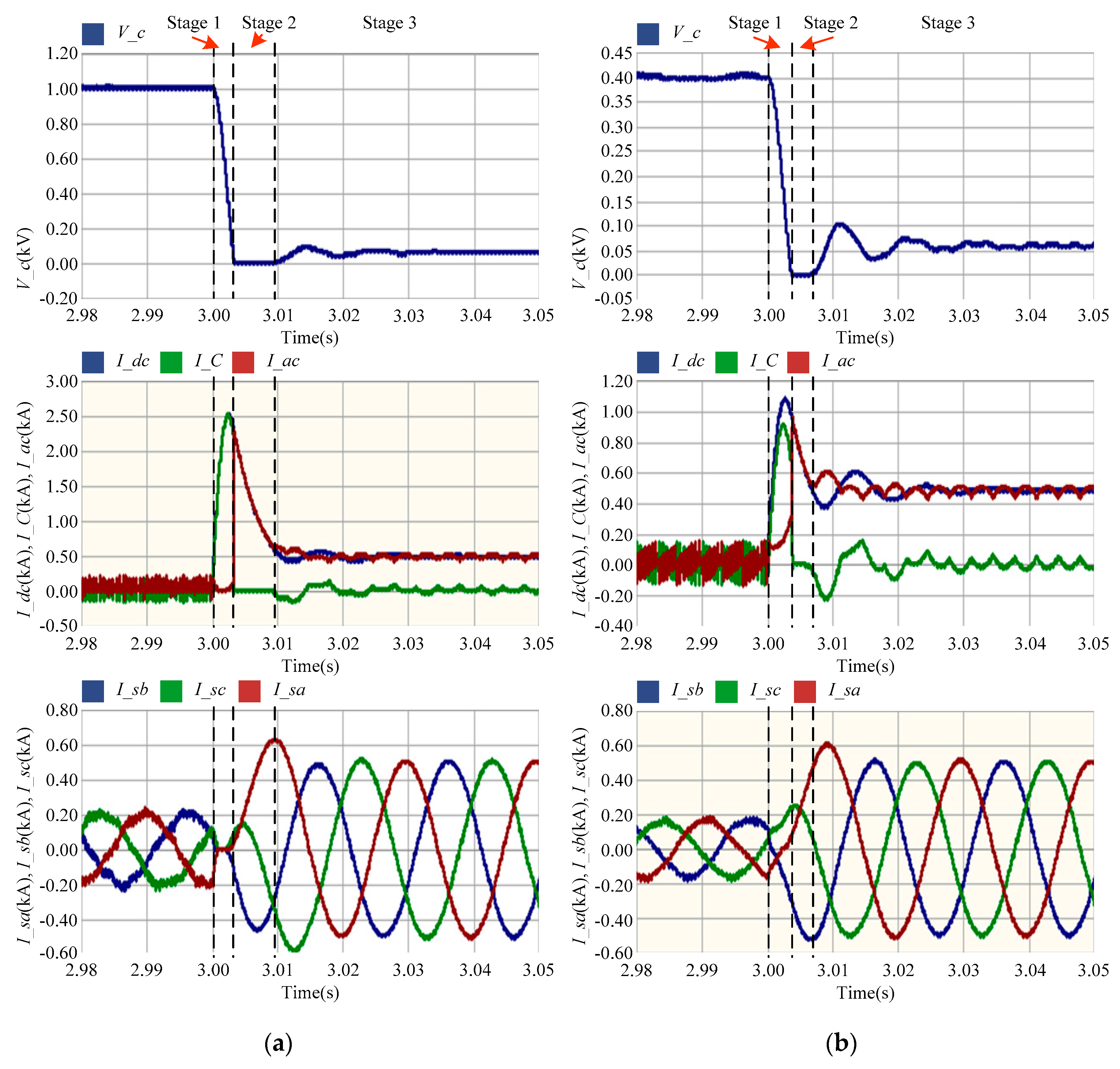
Figure 3.
The equivalent circuit for analysis: (a)The simplified circuit model of VSC; (b) The current path and direction.
Figure 3.
The equivalent circuit for analysis: (a)The simplified circuit model of VSC; (b) The current path and direction.

Figure 4.
The waveform of steady-state quantities in Figure 3: Idc, I1, I2, and I6 (in kA); Udc, Uabl, Uabs and Uan (in kV).
Figure 4.
The waveform of steady-state quantities in Figure 3: Idc, I1, I2, and I6 (in kA); Udc, Uabl, Uabs and Uan (in kV).
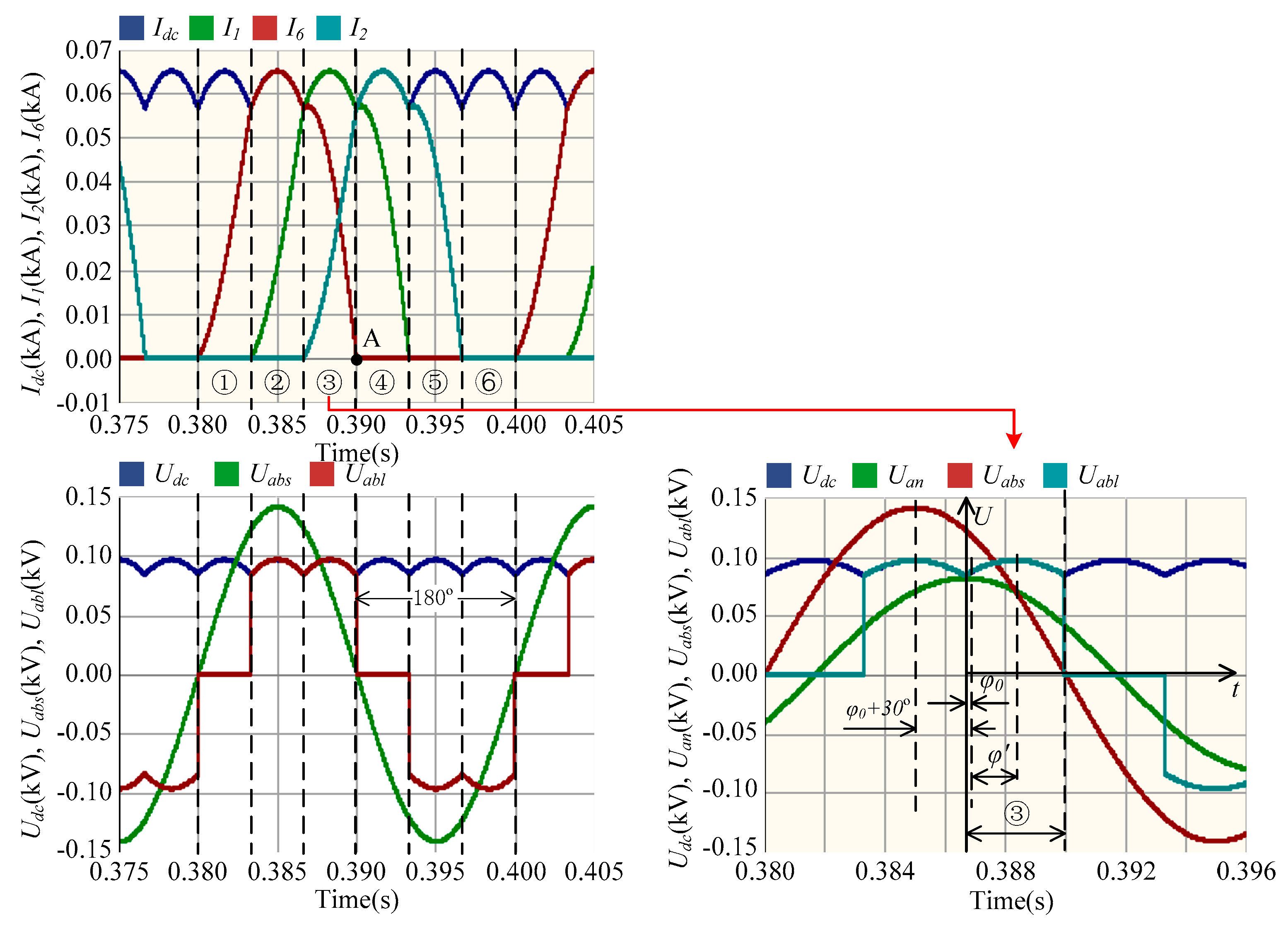
Figure 5.
The equivalent transient-state circuit model of VSC: (a) the natural response process equivalent circuit; and (b) the forced response process equivalent circuit.
Figure 5.
The equivalent transient-state circuit model of VSC: (a) the natural response process equivalent circuit; and (b) the forced response process equivalent circuit.

Figure 6.
The equivalent convert of the RLC circuit.
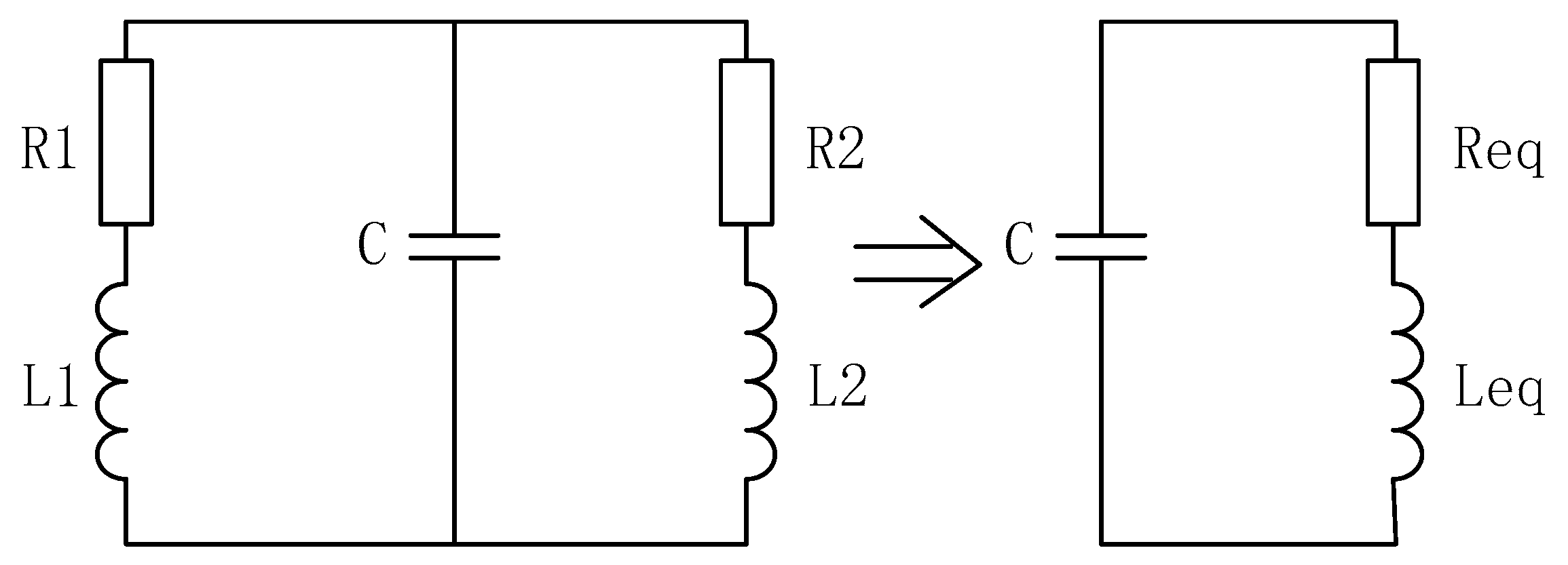
Figure 7.
The waveform of the surge current of simulated values; theoretical values in [4] and this paper.
Figure 7.
The waveform of the surge current of simulated values; theoretical values in [4] and this paper.
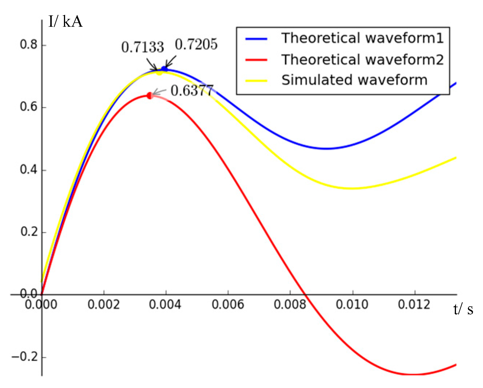
Figure 8.
The structure of a multi-terminal loop-type DC distribution network.

Figure 9.
Switch operations of the classical handshaking method: (a) Switches state after step 2; (b) Switches state after step 4.
Figure 9.
Switch operations of the classical handshaking method: (a) Switches state after step 2; (b) Switches state after step 4.
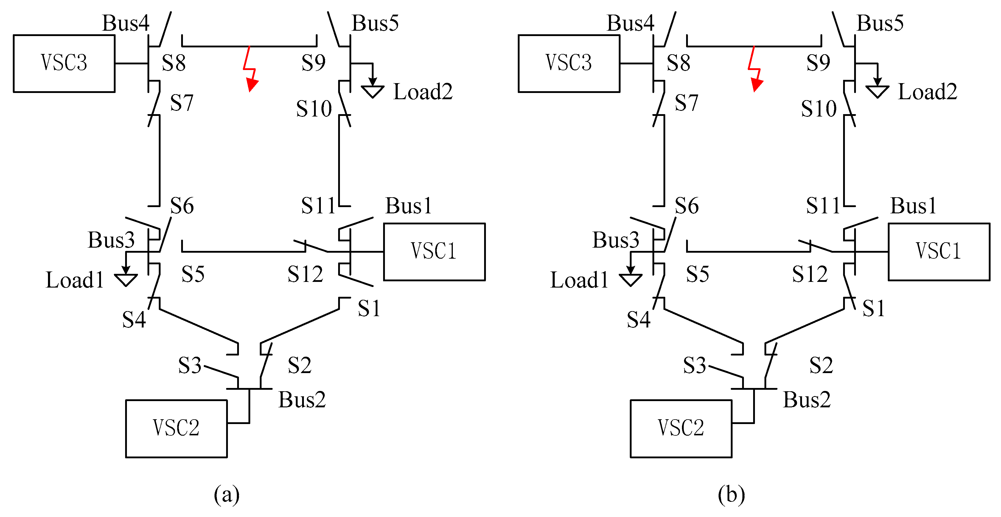
Figure 10.
Switch operations of the improved handshaking method: (a) Switches state after step 2; (b) Switches state after step 4.
Figure 10.
Switch operations of the improved handshaking method: (a) Switches state after step 2; (b) Switches state after step 4.


Table 1.
Simulation parameters and computed initial values.
| System Components | Value | System Voltage | Value |
|---|---|---|---|
| AC-side Inductance Lac | 1.5 mH | Phase Voltage Up_p | 220 V |
| AC-side Resistance Rac | 0.3 Ω | Line Voltage Ul_l | 380 V |
| DC-linked Capacitance C | 6 mF | Equivalent DC Source Udc | 513 V |
| DC-side Inductance Ldc | 0.56 mH/km | Initial DC voltage V0 | 400 V |
| DC-side Resistance Rdc | 0.12 Ω/km |
Table 2.
Simulation parameters and computed initial values.
| Fault Distance (km) | 1 | 2 | 3 | 4 | 5 |
|---|---|---|---|---|---|
| Simulation steady-state current (kA) | 0.480 | 0.445 | 0.411 | 0.380 | 0.351 |
| Theoretical steady-state current (kA) | 0.513 | 0.471 | 0.433 | 0.398 | 0.368 |
| Error (%) | 6.78 | 5.88 | 5.33 | 4.85 | 4.75 |
| Simulation transient-state peak current (kA) | 1.078 | 0.713 | 0.556 | 0.464 | 0.402 |
| Theoretical transient-state peak current1 (kA) | 1.087 | 0.721 | 0.564 | 0.475 | 0.416 |
| Error (%) | 0.91 | 1.06 | 1.51 | 2.32 | 3.52 |
| Theoretical transient-state peak current2 (kA) | 0.994 | 0.638 | 0.486 | 0.398 | 0.339 |
| Error (%) | 7.75 | 10.56 | 12.67 | 12.62 | 15.59 |
Table 3.
Results for the proposed location method.
| Fault Distance/m | 500 | 1000 | 1500 | 2000 | 2500 | 3000 |
|---|---|---|---|---|---|---|
| d/m (Rf = 0) | 519 | 1015 | 1539 | 2054 | 2589 | 3130 |
| Error (%) | 0.63 | 0.50 | 1.30 | 1.80 | 2.97 | 4.33 |
| d/m (Rf = 0.5 Ω) | 579 | 1114 | 1653 | 2190 | 2769 | 3366 |
| Error (%) | 2.63 | 3.80 | 5.13 | 6.33 | 8.97 | 12.20 |
Table 4.
Results for the improved proposed location method.
| Fault Distance/m | 500 | 1000 | 1500 | 2000 | 2500 | 3000 |
|---|---|---|---|---|---|---|
| d/m (Rf = 0) | 519 | 1012 | 1507 | 2016 | 2520 | 3032 |
| Error (%) | 0.63 | 0.40 | 0.23 | 0.53 | 0.67 | 1.07 |
| d/m (Rf = 0.5 Ω) | 536 | 1049 | 1564 | 2089 | 2620 | 3160 |
| Error (%) | 1.20 | 1.63 | 2.13 | 2.97 | 4.00 | 5.33 |
© 2018 by the authors. Licensee MDPI, Basel, Switzerland. This article is an open access article distributed under the terms and conditions of the Creative Commons Attribution (CC BY) license (http://creativecommons.org/licenses/by/4.0/).
Share and Cite
MDPI and ACS Style
Xue, S.-M.; Liu, C. Line-to-Line Fault Analysis and Location in a VSC-Based Low-Voltage DC Distribution Network. Energies 2018, 11, 536. https://doi.org/10.3390/en11030536
AMA Style
Xue S-M, Liu C. Line-to-Line Fault Analysis and Location in a VSC-Based Low-Voltage DC Distribution Network. Energies. 2018; 11(3):536. https://doi.org/10.3390/en11030536
Chicago/Turabian StyleXue, Shi-Min, and Chong Liu. 2018. "Line-to-Line Fault Analysis and Location in a VSC-Based Low-Voltage DC Distribution Network" Energies 11, no. 3: 536. https://doi.org/10.3390/en11030536
Note that from the first issue of 2016, this journal uses article numbers instead of page numbers. See further details here.