Modified Differential Evolution Algorithm: A Novel Approach to Optimize the Operation of Hydrothermal Power Systems while Considering the Different Constraints and Valve Point Loading Effects

Abstract

This paper proposes an efficient and new modified differential evolution algorithm (ENMDE) for solving two short-term hydrothermal scheduling (STHTS) problems. The first is to take the available water constraint into account, and the second is to consider the reservoir volume constraints. The proposed method in this paper is a new, improved version of the conventional differential evolution (CDE) method to enhance solution quality and shorten the maximum number of iterations based on two new modifications. The first focuses on a self-tuned mutation operation to open the local search zone based on the evaluation of the quality of the solution, while the second focuses on a leading group selection technique to keep a set of dominant solutions. The contribution of each modification to the superiority of the proposed method over CDE is also investigated by implementing CDE with the self-tuned mutation (STMDE), CDE with the leading group selection technique (LGSDE), and CDE with the two modifications. In addition, particle swarm optimization (PSO), the bat algorithm (BA), and the flower pollination algorithm (FPA) methods are also implemented through four study cases for the first problem, and two study cases for the second problem. Through extensive numerical study cases, the effectiveness of the proposed approach is confirmed.

1. Introduction

An electrical power system is mainly composed of thermal and hydro power plants connected via transmission lines in order to supply electricity to loads such as industrial zones or manufacturers, etc. For electrical generation, thermal plants use fossil fuel including gas, coal, and oil, which are very expensive, and will become exhausted in the near future, whereas taking water from natural rivers and discharging it via hydro turbines is considered negligible in terms of generation costs. In addition, comparing the response speed to electrical load changes, hydropower plants have advantages over thermal plants, because they can move from producing a very small amount of power to full power in several minutes, due to the quick water control. On the contrary, the startup and the response speed of thermal plants to load changes is very slow. Therefore, thermal plants need to run continuously for some hours once they start. Based on the advantages and disadvantages analyzed for thermal and hydropower plants, it is clear that the coordination of thermal and hydropower plants in electrical generation operations becomes more effective and economical. In summary, hydrothermal scheduling (HTS) aims to minimize the electricity generation fuel cost of thermal plants using fossil fuels, while all constraints from thermal plants, hydropower plants and the system are exactly met [1]. With regard to this problem, the thermal power plant constraints are easily met, because only limitations on generation are taken into consideration and other constraints such as fossil fuel constraints and fuel costs for the start-up and shutdown processes are neglected. Among the optimization problems related to the optimal scheduling of hydrothermal systems, the fixed-head, short-term HTS problem has been widely and successfully studied so far [1,2,3,4,5,6,7,8,9,10,11,12,13,14,15,16,17,18,19,20,21,22,23,24,25,26,27,28,29]. The fixed-head, short-term HTS problem has been classified into two sub-problems with different hydraulic constraints, namely the amount of discharged water available via the turbine [1,2,3,4,5,6,7,8,9,10,11,12,13,14,15,16,17] and reservoir volume limits [2,3,18,19,20,21,22,23,24,25,26,27,28,29,30,31,32,33,34]. In the two sub-problems, the water head of reservoirs is not supposed to be changed over the scheduled time, thus the water discharge function of the two problems has the same quadratic function model with respect to hydro generation and coefficients; however, the set of hydraulic constraints taken into account in the problems are almost completely different. The water volume, which is allowed to run the hydro turbines over the scheduled horizon, is constrained in the first problem, while the main constraints considered in the second problem are the reservoir volume at the beginning and the end of the scheduled horizon, the limitations of the reservoir volume and the water balance in each reservoir.

Several methods have been used to solve the first problem, such as Powell’s hybrid method [1]; the Newton–Raphson method [1,2]; the lambda–gamma method (λ-γ method) [2]; the Lagrange-multiplier, factorization-based, Newton–Raphson method [3]; the Lagrange method based on the linearization of the coordination equation (LCEL) [4]; the Lagrangian relaxation approach [5]; Hopfield neural networks (HNN) [6]; evolutionary programming (EP) [7,8]; the artificial immune system method (AIS) [8]; particle swarm optimization (PSO) and the differential evolutionary method (DE) [8]; the modified bacterial foraging algorithm (MBFA) [9]; the optimal gamma-based genetic algorithm (OGB-GA) [10]; fast genetic algorithm (FGA) [11]; the predator–prey optimization technique (PPO) [12]; improved genetic with multiplier updating (IGA-MU) [13]; real-coded genetic algorithm (RCGA) [14]; a Hopfield Lagrange network (HLN) [15]; an augmented Hopfield Lagrange network (ALHN) [15]; the Cuckoo search algorithm (CSA) [16,17]; and a modified cuckoo search algorithm (MCSA) [17]. On the other hand, there has also been a number of methods proposed to solve the second problem, such as gradient search (GS) [2]; Newton’s method [3]; the simulated annealing approach (SA) [18]; evolutionary programming (EP) [19,20,21]; genetic algorithms (GA) [22]; fast EP (FEP) [23]; improved fast EP (IFEP) [23]; hybrid EP (HEP) [24]; PSO [25]; the improved bacterial foraging algorithm (IBFA) [26]; self-organizing, hierarchical PSO [27]; running improved fast EP (RIFEP) [28]; improved PSO [29,30]; a clonal selection algorithm (CS) [31]; fully-informed particle swarm optimization (FIPSO) [32]; a cuckoo search algorithm with Lévy distribution (CSA-Lévy) [33]; a cuckoo search algorithm with Lévy Gaussian distribution (CSA-Gauss) [33]; a cuckoo search algorithm with Cauchy distribution (CSA-Cauchy) [33]; a one rank cuckoo search algorithm with Lévy distribution (ORCSA-Lévy) [34]; and a one rank cuckoo search algorithm with Cauchy distribution (ORCSA-Cauchy) [34].

Among the introduced methods, the methods in [1,2,3,4,5,6,15] are in the family of deterministic algorithms and the others in [7,8,9,10,11,12,13,14,16,17,18,19,20,21,22,23,24,25,26,27,28,29,30,31,32,33,34] are in the family of meta-heuristic algorithms. The first method group is mainly based on the gradient to find the optimal solution. Meanwhile the second method group searches for the optimal solution mainly based on the population. Moreover, the methods in the first group are defined as derivative-based optimization methods, finding the optimal solution by a single path search line and suffering from the drawback that they cannot deal with non-convex problems where the objective functions or constraints of the problems are non-differentiable or nonlinear. In addition, the conventional methods also suffer from difficulties when dealing with large-scale problems with complicated constraints. On the contrary, the meta-heuristic methods initialize a set of solutions at the beginning of the optimal solution search process. The solutions are newly generated in each iteration and the quality of these solutions is evaluated via a fitness function consisting of a penalty amount for constraint violation and an objective function that needs to be minimized. Unlike the deterministic algorithms, the entire computation procedure of many meta-heuristic methods will terminate based on a predetermined maximum number of iterations. The obtained solutions are capable of satisfying all constraints as the current iteration is much lower than the maximum number and the solution might be out of feasible operating zones even if the termination criteria has already been reached. The meta-heuristic algorithms are considered stronger and more effective than deterministic algorithms, because they can deal with problems where non-differentiable objective functions and many nonlinear constraints as well as large-scale systems are taken into consideration.

Among the deterministic methods, HLN and ALHN are considered the most effective methods, since they can obtain the global optimum solution with a very fast execution time and a low number of fitness evaluations. HLN is a developed version of HNN that combines the Hopfield network from the HNN method and the Lagrange optimization function of the λ-γ method. The search process of the HLN method is based on calculating the change of dynamic neurons, and the updating input and output of multiplier neurons and continuous neurons after establishing an energy function from the Lagrange optimization function. ALHN is also an improved version of HLN since the Lagrange optimization function is converted into an augmented Lagrange function. HLN can overcome several of the drawbacks of HNN, such as local optimum solutions, low convergence, and limited applications for large-scale systems. Compared to HLN, ALHN can obtain better optimum solutions. However, ALHN contains more control parameters due to its converting the Lagrange function into an augmented Lagrange function. In spite of the good performance, the application of the two methods must be stopped when facing problems with many considered constraints, since it has a high number of control parameters that are directly proportional to the number of considered constraints. Furthermore, there is a sensitive impact of the parameters on the results. Thus, if the value of a parameter is tuned, other parameters should also be changed. As a result, the selection of the parameters is the big challenge for the two methods.

Among the meta-heuristic algorithms, SA is the worst method for searching for the optimal solution for hydrothermal system scheduling problems. In fact, although SA can tackle the applicability limitations for non-differential objective functions that deterministic methods have coped with thus far, SA has not been widely applied because it requires a long simulation time and obtains a low quality solution. The applicability of SA is significantly dependent on the selection of the initial temperature and the cooling rate value. The optimal temperature is very hard to determine, since it has a very large range, from zero to infinite, while the cooling rate is used to decrease the temperature and is calculated based on the temperature. For the implementation of GA, the diversification of the offspring in the crossover operation and mutation operation must be performed to guarantee an optimal solution. This manner is regarded as an advantage of the EP method, as the main search operator generating new solutions is fulfilled by the mutation operation. Contrary to GA, EP is slow to obtain a near-optimal solution. However, the convergence speed of EP and GA can be improved by adding other techniques. In fact, there have been several improvements applied to these methods to enhance their search ability and speed up their convergence process. Several improved versions of GA and EP have been developed in [10,11,13,14,23,24,28]. The reported results indicate that the improvements in the conventional EP and GA are successful and efficient. However, there are some weak points, such as the high number of iterations, long execution time, and low quality of optimal solutions. Aware of the drawbacks of GA, the authors in [10] proposed the OGB-GA method by combining the Lagrange optimization function and GA in order to decrease the number of control variables for GA. Instead of having a large number of control variables, such as hydro generations and thermal generations, OGB-GA uses only one gamma variable from the Lagrange optimization function. Thus, GA is used in OGB-GA to determine gamma and then the coordination equation in the λ-γ method is applied to calculate the generation of hydro and thermal units. The result comparisons in [10] illustrate the better performance of OGB-GA compared to GA. However, OGB-GA cannot deal with systems where the non-convex fuel cost function is taken into account. In [11], FGA has been indicated as more efficient than GA in terms of higher solution quality and shorter computation times for solving large-scale systems via the result comparisons on four systems. Compared to GA, FGA has focused on decreasing the search space by collecting the minimum error and the maximum error of the best individual and the worst individual among the current population. As a result, FGA could carry on the search around the narrow zone and then an optimum could be obtained quickly, with a low maximum iteration number. However, if a global optimal solution was outside the limited narrow zone, FGA could converge to a local optimum due to the premature convergence. This disadvantage is evidence of the restricted application of FGA. Compared to FGA and OGB-GA, IGA-MU and RCGA show better performance and wider applications for optimization problems in electrical engineering.

In the EP methods introduced in [19,20,21], only the Gauss random variable was used to generate offspring and the scaling factor was regarded as a constant. However, in the improved versions of EP [23,28], the number of offspring was generated by randomly generated initial parents using Gauss or Cauchy mutations in addition to using the scaling factor as a variable during the search process. The improved EP methods improved the solution and sped up convergence and were superior to conventional EP via only one test system. The improvement of HEP has not been validated, although the authors stated that their improved method was better than original one. In fact, only one system with one thermal unit and one hydro unit scheduled in six twelve-hour subintervals and quadratic fuel cost functions of thermal units were employed to run the proposed methods. Moreover, the optimal solutions for the simple system reported have indicated that the water discharge was lower than the minimum value predetermined in problem data.

Compared to GA and EP, PSO is more easily implemented for the HTS problem, since its feature is very simple, consisting of two updated factors, namely the velocity and position. Furthermore, the solution and the computation for PSO are more effective than those for GA and EP. Recently, several applications of CSA for HTS problems in [16,17] for the first problem and in [33,34] for the second problem have shown very good results with fast execution times compared to GA variants, EP variants, and other methods such as AIS, DE and deterministic methods. CSA methods construct their search strategy based on Lévy flights and the probability of alien egg identification. Lévy flights act as a global search tool, while the probability of alien egg identification acts as a local search tool. Thus, in each iteration, CSA methods have produced two new solution generations in which global search is the first generation and the probability of alien egg identification is the second generation. Compared to other mentioned methods, CSA methods can enlarge the global zone by using Lévy flights and then a local search around the solutions that have just been found by the global search could effectively exploit a narrow zone. As shown in [33,34], CSA could use three different distributions such as Lévy distribution, Gaussian distribution and Cauchy distribution, but the most appropriate distribution was Lévy distribution. Although the evidence indicates that a good evaluation of CSA has been clearly shown, the CSA methods used a high total number of fitness evaluations because they had two separate search strategies.

The CDE was developed by Storn and Price in 1997 [35]. CDE, one of the most popular meta-heuristic algorithms, has been applied to solving different optimization problems in electrical engineering fields, such as hydrothermal scheduling [8], large-scale distribution systems [36], economic dispatch problems [37], and optimal reactive power dispatching [38]. CDE has been considered a simple meta-heuristic algorithm with two main advantages when compared to GA, and has been applied to optimization problems such as fast convergence and few control parameters [39]. In spite of the advantages and the wide applicability of CDE, it has still coped with many other drawbacks, such as feeble local search ability, low convergence to the global optimum, and being easily trapped in local optima and less diversity [40]. As is known, DE has three main operations, including mutation operation, crossover operation and selection operation. The mutation operation generates new solutions, the selection operation keeps the promising current solutions, and crossover mixes old solutions and new solutions to carry out the next mutation. Thus, many studies have pointed out the disadvantages of DE, mainly derived from the mutation and selection operations. In their study [41], Qin et al. analyzed the mutation operation and pointed out the limits of the operation. It was shown that the mutation operation of CDE with the task of selection of mutation factor had a significant impact on the performance of DE. Thus, the implementation of CDE was time consuming due to the number of trials needed to select the mutation factor [41]. In order to overcome disadvantages of CDE, Qin et al. suggested several improved versions of the mutation. Unlike the study in [41], Padhye et al. [42] focused on the selection operation and suggested the elitist selection operation because its performance influences the next mutation in the next generation. The selection of CDE may lead to missing some promising solutions, which are abandoned, and whose qualities would be better than other retained solutions. In fact, CDE selection is a comparison between the previous solution X_d and the solution Z_d, which was chosen via crossover. Derived from the indication of the limitations of CDE, many DE variants have been constructed by modifying mutation and selection operation such as DE with the adaptive mutation [40,41], DE with elitist selection [42], DE with ancestor tree [43], DE with adaptive mutation and elitist selection [44], DE with a penalty method [45], and surrogate differential evolution (SDE) [46]. DE variants with adaptive mutation and/or elitist selection can find better solutions than CDE; however, these methods have to cope with fundamental limitations such as spending a great deal of time tuning the crossover factor and several factors in the adaptive mutation operation, missing promising solutions of good quality, and keeping identical solutions in the current population.

The analysis of the good and bad properties of all mentioned methods identifies drawbacks that these methods have addressed, such as the:

(i)

Restriction of applicability to complicated systems with non-differential objective functions and a high number of power plants,

(ii)

Convergence to local optimal solutions or near-global optimal solutions with low quality and high objective functions, and

(iii)

Limited time for searching for the optimal solution due to a high number of iterations and for tuning control parameters due to high number of control parameters and a large range of such control parameters.

In this study, we propose an efficient and new modified differential evolution (ENMDE) with two main modifications to the two operations, in which the first modification, self-tuned mutation, is constructed on the mutation operation, and the second modification, leading group selection, is carried out in the selection operation. The main contributions to the improvement of the proposed ENMDE method are as follows:

(i)

Propose the cancelling of crossover operations in order to skip the task of tuning the crossover factor. This suggestion can enable the proposed method reduce the impact of parameter factors on the results and reduce the simulation time for the tuning crossover factor.

(ii)

Propose a new formula for calculating the average fitness distance ratio in the mutation operation, which can balance the global search and local search for the proposed method effectively. In addition, the formula can reduce the selection of the average fitness distance ratio that most previous studies have coped with and the formula helps to reduce the simulation time for tuning good value.

(iii)

Propose the leading group selection technique to keep the best solutions among old solutions and new solutions, where only one out of the identical good solutions is retained and solutions of worse quality are abandoned. The technique provides good opportunities to produce more new solutions of high quality.

In order to test the performance of the proposed ENMDE, we implement the ENMDE and two other versions of DE, including DE with self-tuned mutation (STMDE) and DE with the leading group selection (LGSDE) to solve two different fixed-head, short-term hydrothermal scheduling problems with six study cases. Between the two problems, the second problem is more complicated than the first, because reservoir constraints such as minimum limit, maximum limit, initial volume, end volume and water balance are considered. Four study cases, including two cases with convex objective functions and two cases with non-convex objective functions in the first problem, and one case with a convex objective function and one case with a non-convex objective function in the second problem, are the challenges that will result in evidence with which to evaluate the performance of the proposed ENMDE.

The remainder of this paper is organized as follow: Section 2 analyzes methodologies relating to the HTS problem. The original differential evolution and proposed methods for the HTS problem are introduced in Section 3. The application of the two considered hydrothermal scheduling problems, case studies, and the discussion of the results are found in Section 4, Section 5 and Appendix A. Finally, the conclusions are stated in Section 6.

2. Methodology Analysis

The aim of the short-term, fixed-head HTS problem is to reduce the total generation fuel cost of thermal units in addition to meeting load power balance, hydraulic, and generator operating limit constraints. The considered hydrothermal system with N₁ thermal units and N₂ hydro units working in M scheduled sub-intervals is mathematically formulated as follows.

2.1. Objective Function

The economy of the HTS mainly depends on the optimization of fuel cost in thermal units, whilst the fuel cost in hydro units is neglected due to the assumption that water from a natural river is free. In fact, the fuel cost function of thermal units has been built and developed, so that it will be approximately close to the practical costs; meanwhile the fuel cost for hydro units has never been considered and mathematically formulated. Consequently, the objective function of the problem aims to reduce the thermal unit costs for the whole scheduled time of M sub-intervals as follows.

$$\mathrm{Min}{C}_T={\displaystyle \sum _{m=1}^M{\displaystyle \sum _{i=1}^{N_1}{t}_m{F}_{im}}}$$

(1)

where F_im is the fuel cost of the ith thermal unit for one hour in the mth subinterval. In the past, a quadratic function has been employed to represent a second order fuel cost function [2]:

$$F_{im}=\left[a_{si}+b_{si}{P}_{si,m}+c_{si}{P}_{si,m}^2\right]$$

(2)

However, during the operation of increasing or decreasing the power output of thermal units, valve effects take place, resulting in a change of efficiency and a different fuel cost function compared to the quadratic one in Equation (2). The new form of the fuel cost function is the sum of a quadratic function and a sinusoidal function [13]:

$$F_{im}=\left[a_{si}+b_{si}{P}_{si,m}+c_{si}{P}_{si,m}^2+\left|d_{si}\times \sin \left(e_{si}\times \left(P_{si}^{\min }-P_{si,m}\right)\right)\right|\right]$$

(3)

2.2. Transmission Grid Constraints and Generator Constraints

Power balance equality constraint: The total energy generated from the hydrothermal system and transmitted to the power grid must be equal to the total load demand and power losses of the system in each subinterval:

$${\displaystyle \sum _{i=1}^{N_1}{P}_{si,m}}+{\displaystyle \sum _{j=1}^{N_2}{P}_{hj,m}}-P_{L,m}-P_{D,m}=0;m=1,\dots ,M$$

(4)

where the power losses in transmission lines are calculated using Kron’s formula [2]:

$$P_{L,m}={\displaystyle \sum _{i=1}^{N_1+N_2}{\displaystyle \sum _{j=1}^{N_1+N_2}{P}_{i,m}{B}_{ij}{P}_{j,m}}}+{\displaystyle \sum _{i=1}^{N_1+N_2}{B}_{0i}{P}_{i,m}}+B_{00}$$

(5)

Limits on power output: Thermal and hydro generations must be between their maximum and minimum values:

$$P_{si,\min }\le P_{si,m}\le P_{si,\max };i=1,\dots ,N_1;m=1,\dots ,M$$

(6)

$$P_{hj,\min }\le P_{hj,m}\le P_{hj,\max };i=1,\dots ,N_2;m=1,\dots ,M$$

(7)

In power system operation, the primary fuels for thermal plants, such as the coal, gas or oil burned to drive thermal turbines, need to be adjusted to the capacity of the thermal generators due to their generation limits. On the contrary, the power generation of hydro units is controlled by handling the water discharge through the turbines.

2.3. Hydraulic Constraints

Available water volume constraint: The total water discharged via hydro turbines over the whole scheduled time horizon is limited by:

$${\displaystyle \sum _{m=1}^M{t}_m{q}_{j,m}}=W_j;j=1,\dots ,N_2$$

(8)

where q_j,m is the rate of water flow via the turbine of hydropower plant j in interval m. Supposing that the hydraulic reservoir is large enough for the water head to be approximately fixed at the same value over the scheduled time period, Glimn–Kirchmayer expressed the water discharge function with respect to the power output of a hydropower plant only as below [2].

$$q_{j,m}=a_{hj}+b_{hj}{P}_{hj,m}+c_j{P}_{hj,m}^2$$

(9)

Limits on water discharge: The amount of water discharged via hydro turbines should be between the boundaries.

$$q_{j,\min }\le q_{j,m}\le q_{j,\max };j=1,2,\dots ,N_2;m=1,2,\dots ,M$$

(10)

where q_j,max and q_j,min are the highest and lowest water discharges via the hydropower plant j.

Dynamic hydraulic constraint:

$$V_{j,m-1}-V_{j,m}+I_{j,m}-Q_{j,m}-S_{j,m}=0$$

(11)

where Q_j,m is the total discharge constraint for each duration of t_m obtained as below:

$$Q_{j,m}=t_m{q}_{j,m}$$

(12)

where q_j,m is water discharge rate obtained using Equation (9).

Initial and final reservoir storage:

$$V_{j,0}=V_{j,initial};V_{j,M}=V_{j,End}$$

(13)

Reservoir storage limits:

$$V_{j,\min }\le V_{j,m}\le V_{j,\max };j=1,2,\dots ,N_2;m=1,2,\dots ,M$$

(14)

where V_j,max and V_j,min are the maximum and minimum reservoir storages of the hydropower plant j, respectively.

Normally, the volume of each reservoir is reported at the beginning of operation planning and during the process the value is supervised so that satisfying limitations between the lowest and the highest values are subject to Equation (14). Based on the demanded power energy and inflow water, the amount of water is obtained at the end of the process. These are completely different from the constraints in Equation (8) above. In this paper, two models of hydraulic constraints are thus taken into account, in which the first model considers only the water available over the scheduled subintervals, whereas the second model considers only a set of constraints related to the volume of reservoirs such as the start volume, the end volume and the limitations on the reservoir volume. Corresponding to the two models, the constraints in Equations (8) and (10) are included in the first model, while a set of constraints consisting of Equations (10), (11), (13) and (14) are included in the second model.

3. Approaches

3.1. Original Differential Evolution

The conventional differential evolution was developed by Storn and Price in 1997 [35]. Similar to other meta-heuristics, CDE also starts with a population of N_p initial solutions and then the solutions are improved and evaluated to choose the best one at each iteration. The main operations of the CDE are as follows.

3.1.1. Initialization

Each individual in the population is represented by X_d = [x_1d, x_2d, …, x_ld, …, x_Dd] where d is the dth solution, d = 1, …, N_p, and D is the number of variables included in each optimal solution.

3.1.2. Mutation Operation

Mutation operation is a phase where new solutions are produced only one time in each iteration. Each old solution is newly updated using three different random solutions and the mutation factor. Among the three random solutions, the main role of one is to search around it, while the two remaining solutions play a sub-role in creating a difference or a distance from the first random one. The expression can be indicated via the following equation.

$$Y_d=X_{r1}+F(X_{r2}-X_{r3})$$

(15)

where X_r1 is the first random solution playing a main role; X_r2 and X_r3 are the second the third random solutions playing a sub-role; and F is the mutation factor ranging from 0 to 2.

3.1.3. Crossover Operation

In order to generate new solutions for the next iteration, there must be a mixture between the current solutions and the previous solutions. This is the crossover operation and is performed by

$$Z_d=\{\begin{array}{ll}{Y}_d& \mathrm{if}ran{d}_d\le CR\\ X_d& \mathrm{otherwise}\end{array}$$

(16)

3.1.4. Selection Operation

The selection operation is carried out to keep the better solutions in the current iteration. The best solution with the lowest fitness function value is then determined based on the evaluation of the fitness function. The selection operation may be mathematically expressed as follows:

$$X_d=\{\begin{array}{ll}{X}_d& \mathrm{if}FT\left(X_d\right)\le FT\left(Z_d\right)\\ Z_d& \mathrm{otherwise}\end{array}$$

(17)

3.2. The Proposed Approach

In the proposed ENMDE method, we propose two new techniques to improve the performance of the mutation operation and the selection operation. The first technique is called the self-tuned mutation technique and the second technique is called the leading group selection technique.

3.2.1. Self-Tuned Mutation Technique

In the mutation operation, CDE uses only two random solutions to generate an increased value for producing new solutions, as shown in Equation (15). The increase based on the two different solutions used during the search process leads easily to a local optimum and the capability for converging to a global optimum is low. Consequently, the conventional mutation has been modified, many formulas have been proposed and the following ones have been popular so far [41].

$$\mathrm{rand}./1:Y_d=X_{r1}+F(X_{r2}-X_{r3})$$

(18)

$$\mathrm{rand}./2:Y_d=X_{r1}+F(X_{r2}-X_{r3}+X_{r4}-X_{r5})$$

(19)

$$\mathrm{best}/1:Y_d=G_{best}+F(X_{r1}-X_{r2})$$

(20)

$$\mathrm{best}/2:Y_d=G_{best}+F(X_{r1}-X_{r2}+X_{r3}-X_{r4})$$

(21)

$$\mathrm{current-to-best}:Y_d=X_d+F(G_{best}-X_d+X_{r1}-X_{r2})$$

(22)

Among the suggestions, rand./1 and rand./2 are mainly focusing on the global search, while best/1 and best/2 mainly focus on the local search. Clearly, the first two are searching solutions operating around all the current solutions with a large search space, while the two continuous solutions exploit the space near the current best solution. Thus, the search space is narrow. This scenario can lead to a limitation of the four formulas, since the first two are effective in the global search ability, but weak in the local search ability, while the two others are weak in the global search but effective in the local search. Consequently, there are possibilities that rand./1 and rand./2 are hard to converge to or slowly converge to a global optimum [47], and best/1 and best/2 can fall into a local optimum easily [48]. Besides this, the current-to-best also opens the search zone similarly to rand./2. Therefore, the impact of current-to-best and rand./2 on the result can be similar.

On the other hand, rand./1 is the conventional mutation of CDE, which has been considered weak and hard to converge to the global solution due to the small increased value obtained by two different random solutions. On the contrary, rand./2 in Equation (19) can enable CDE to come to a larger search zone when the increased value is from four random solutions. However, the larger step will open the search space when the search procedure begins. Obviously, if the use of rand./1 and rand./2 is separated, the modified mutation will not be effective. The best/1 and best/2, as shown in Equations (20) and (21), are respectively special cases of rand./1 and rand./2 if the first random solution X_r1 and the best solution G_best are the same. Consequently, if Equations (20) and (21) are used separately, the performance of the modification may be insignificantly improved.

Derived from the analysis above, it can be implied that if either Equations (18) and (19) or Equations (20) and (21) are used as a pair, either the global search or the local search will be focused independently and the modifications will suffer from several drawbacks, such as slow convergence to the global optimum solution and easily obtaining the local optimum solution. In fact, exploration and exploitation are the two main phases for an algorithm to quickly converge to the global optimum solution and if one of them is omitted, limitations will be present [49]. Thus, balancing exploration and exploitation is very necessary and the combination of the two random versions and two best versions needs to be carried out. In [50], the authors developed a composite DE (CoDE) using three mutation versions consisting of rand./1, rand./2 and current-to-rand./1, in which current-to-rand./1 had the approximate mode with current-to-best, but G_best was replaced with another random solution.

The use of one of them is based on different mutation factor values and crossover factors. The method seems to be simple to implement but its effectiveness is promising since it can obtain better results than other DE variants. In spite of the favorable results, the suggested CoDE has not completely persuaded authors because its application has been performed only on benchmark functions with simple objective functions and without complicated sets of constraints. In their study [41], Qin et al. employed all the modified mutation versions without fixed conditions, together with the use of another modified crossover operation and a conventional selection operation to construct self-adaptive DE (ASDE). The ASDE has also been demonstrated better than other DE variants via comparisons with benchmark functions. Unlike [41,50], the authors in [44] developed an adaptive elitist DE (AEDE) with an adaptive mutation operation and an elitist selection operation, and implemented the AEDE in six cases of optimization problems with truss structures with discrete design variables. The problem is a bigger challenge than benchmark functions, since objective functions as well as the related expressions are much more complicated than those from benchmark functions. This adaptive mutation operation used only rand./1 and current-to-best for two predetermined conditions based on the comparison between the fitness ratio (FR) and a predetermined tolerance (ε). The FR is a ratio of the difference of the fitness function of each solution and the average fitness function of all populations to the best fitness function of the best solution. If the FR is higher than ε, rand./1 is employed, otherwise the current-to-best is more appropriate. The AEDE has been divided into ADE (DE with the adaptive mutation) and EDE (DE with elitist selection) and this has resulted in three versions of DE. Among the DE variants, AEDE has been considered more effective for the global optimum solution and faster for convergence with a lower maximum number of iterations.

In our paper, we propose a self-tuned mutation based on the four modified mutation versions consisting of rand./1, rand./2, best/1 and best/2, in which rand./1 and rand./2 are included in the first group, called rand group, and best/1 and best/2 are included in the second group, called best group. The condition determining whether to apply either rand group or best group for each solution under consideration d is dependent on the fitness distance ratio (∆FT_d) of the considered solution to the best solution and the average fitness distance ratio (∆FT_mean). ∆FT_d has been proposed in [41], while ∆FT_mean is first proposed for our proposed DE in the study. They are expressed in the following models.

$$\Delta F{T}_d=\frac{F{T}_d-F{T}_{best}}{F{T}_{best}}$$

(23)

$$\Delta F{T}_{mean}=\frac{\frac{\left({\displaystyle \sum _{d=1}^{N_p}F{T}_d}\right)}{N_p}-F{T}_{best}}{F{T}_{best}}$$

(24)

where FT_d and FT_best are the fitness function of the solution under consideration d and the fitness function of the best solution among the current population.

When the ∆FT_d is higher than ∆FT_mean, the rand group is used. Otherwise, the best group is chosen instead. On the other hand, the condition for the use of each solution in the rand, group and each solution in the best group should be also established. Thus, we propose a mutation mode factor (MMF) and the comparison of a random number with MMF is the decision for use. The proposed complete self-tuned mutation is described in detail in pseudo code in Algorithm 1.

Algorithm 1: Self-tuned mutation technique
If	∆FTd > ∆FTmean            % the first condition
	If  randd. > MMF            % the second condition
	$Y_d=X_{r1}+F(X_{r2}-X_{r3})$        % rand./1
	else
	$Y_d=X_{r1}+F(X_{r2}-X_{r3}+X_{r4}-X_{r5})$    % rand./2
	End
else	% the first condition
	if   randd. > MMF           % the second condition
	$Y_d=G_{best}+F(X_{r1}-X_{r2})$       % best/1
	else
	$Y_d=G_{best}+F(X_{r1}-X_{r2}+X_{r3}-X_{r4})$   % best/2
	end
end

3.2.2. Leading Group Selection Technique

As mentioned, most methods have tended to improve the performance of the mutation technique rather than crossover and selection, except the study in [47] that modifies the crossover, the study in [42] that develops an elitist selection operation, and the study [44] that applies the elitist selection operation, although the selection operation plays a very important role in improving the solution quality. In fact, the elitist selection operation has been tested on benchmark functions [42] and in an optimization design problem [44], and the surprising results indicate that the elitist selection is much better than the convention selection in conventional DE in terms of the minimum value and the standard deviation value. In elitist selection, X = [X₁, X₂, …, X_d, …, X_Np] and Z = [Z₁, Z₂, …, Z_d, …, Z_Np] are integrated into one group and then N_p best solutions are retained and assigned to X, which will be used for the next mutation to produce a new solution in the next iteration. Note that Z_d has been obtained by a crossover operation, by choosing either X_d or Y_d. The crossover in Equation (16) indicates that if CR is much less than 1, most of new solutions Y_d in mutation operation are abandoned and most of X_d will be retained instead. Therefore, the probability that X and Z are the same in the elitist selection is very high, and the overlapping solutions are kept by the elitist selection. Therefore, to avoid the overlapping solutions, CR should be set to 1 with the aim of receiving all new solutions in the mutation and to have N_p new solutions different from N_p old solutions. This means that Z_d is always Y_d, and X_d and Z_d in the elitist selection are completely different. Thus, in our selection operation we also use the main idea from elitist selection with some modifications; the proposed technique is given in Algorithm 2.

When applying the proposed selection technique, our proposed ENMDE can be superior to other DE variants, as it has the following advantages:

(i)

It does not perform a crossover operation, reducing the computational time and reducing the number of trial runs for different CR values;

(ii)

It exploits all new solutions generated from the mutation operation; and

(iii)

It keeps N_p leading solutions, which are completely different from other solutions.

Algorithm 2: Leading group selection technique

(1) Integrate both old solutions X and new solutions Y into one group, called W W = X&Y = [X1, X2, …, Xd, …, XNp, Y1, Y2, …, Yd, …, YNp] (2) Sort the new set of solutions with 2xNp solutions. The solution with the lower fitness function is put on the left and the solution with the higher fitness function is put on the right. (3) Identify identical solutions, keeping one of them and abandoning the remaining ones. (4) Keep the Np leading different solutions with lower fitness than the abandoned ones.

3.3. The Iterative Procedure of the Proposed ENMDE

The whole search of the proposed ENMDE is shown in Algorithm 3. Note that the crossover operation is omitted in the algorithm.

Algorithm 3: The proposed efficient and new modified differential evolution

Select Np, Gmax, F, and MMF   Initialization X = [X1, X2, …, Xd, …, XNp];   Evaluate the initial solution FT(X) = [FT(X1), FT(X2), …, FT(Xd), …, FT(XNp)]   Determine the best solution with the lowest fitness function: Gbest, FTbest While G < Gmax   Calculate ∆FTd for each solution Xd   Perform Algorithm 1 to obtain solutions Y % mutation operation   Evaluate fitness function for solutions Y   Perform Algorithm 2   % selection operation   Determine the best solution with the lowest fitness function: Gbest, FTbest End

4. Application to Two Considered Hydrothermal Scheduling Problems

4.1. Initialization and Handling Equality Constraints

In the considered HTS problems, two sets of variables, including control variables and dependent variables, are considered. The control variables will be generated randomly at the beginning and automatically updated during the search process based on the proposed method, whereas the independent variables are calculated from the equality constraints so that the objective function can be minimized. Some control variables and all independent variables are usually included in the fitness function to allow the evaluation of the quality of a solution. Normally, the control variables will be present in the objective function term and the appearance of independent variables is in the penalty terms. The sum of the two kinds of term is the fitness function, and an optimal solution must have the minimum objective function value and the zero value of the penalty terms. Due to their dealing with different problems, the control and the independent variables are also different corresponding to the typical problems, but the fitness function can be identical if they have the same objective function and independent variables.

For the first problem: In the first problem considered in this paper, each solution X_d (d = 1, …, N_p) contains the control variables, including the generation of thermal units P_si,m,d and water discharge of hydro units q_j,m,d in subintervals. However, in order to satisfy the available water constraint and power balance constraint, the control variables included in solution d are comprised of the power generation of (N − 1) thermal units (from unit two to unit N₁) over all M subintervals and the water discharge from all hydropower plants over the first (M − 1) subintervals. The population is randomly initialized within the feasible operating zone of all units as follows.

$$P_{si,m,d}=P_{si,\min }+rand.(P_{si,\max }-P_{si,\min });i=2,\dots ,N_1;m=1,\dots ,M$$

(25)

$$q_{j,m,d}=q_{j,\min }+rand.(q_{j,\max }-q_{j,\min });j=1,\dots ,N_2;m=1,\dots ,M-1$$

(26)

The water discharge of each hydro unit q_j,M,d in the last subintervals is then calculated using (8), as follows:

$$q_{j,M,d}=(W_j-{\displaystyle \sum _{m=1}^{M-1}{t}_m{q}_{j,m,d})/t_M}$$

(27)

All hydro unit generations in M subintervals are calculated as below:

$$P_{hj,m,d}=\frac{-b_{hj}\pm \sqrt{b_{hj}^2-4c_{hj}(a_{hj}-q_{j,m,d})}}{2c_{hj}};m=1,\dots ,M;j=1,\dots ,N_2$$

(28)

As a result, we obtained the power output of thermal units from unit two to unit N₁ and the power output of all hydro units so far. Finally, the power balance constraint Equation (4) will be satisfied by the power output of the independent variable (power output of thermal unit one), which is calculated as follows [16,17]:

$$P_{s1,m,d}=P_{D,m}+P_{L,m}-{\displaystyle \sum _{i=2}^{N_1}{P}_{si,m,d}}-{\displaystyle \sum _{j=1}^{N_2}{P}_{hj,m,d}}$$

(29)

For the second problem: Similarly, the control variables consisting of a power output of (N₁ − 1) thermal units in each subinterval and reservoir volumes of all hydro units in the first (M − 1) subintervals and independent variables such as the total water discharge in each subinterval in this problem are chosen to satisfy the equality constraints such as power balance and continuity of water equality. Each solution in the population is represented as [P_si,m,d, V_j,m,d] and they are also randomly generated by:

$$P_{si,m,d}=P_{si,\min }+rand.(P_{si,\max }-P_{si,\min });i=2,\dots ,N_1;m=1,\dots ,M$$

(30)

$$V_{j,m,d}=V_{j,\min }+rand.(V_{j,\max }-V_{j,\min });j=1,\dots ,N_2;m=1,\dots ,M-1$$

(31)

The total water discharge over the t_m hours is then calculated using (11) above, as follows.

$$Q_{j,m}=V_{j,m-1}-V_{j,m}+I_{j,m}-S_{j,m};m=1,\dots ,M$$

(32)

The water discharge q_j,m is calculated using Equation (12) and then the hydro generation P_hj,m can be obtained using Equation (28). Finally, the generation of thermal unit one is determined by Equation (29).

4.2. Fitness Function Evaluation

Each solution needs to be evaluated after every iteration. Therefore, the evaluation is performed based on the fitness function, which is the sum of the objective function and the amount of penalties for dependent variables of slack thermal unit one and water discharge in the Mth subinterval. Generally, the fitness function for the two considered problems is as below [16].

$$F{T}_d={\displaystyle \sum _{m=1}^M{\displaystyle \sum _{i=1}^{N_1}{F}_i(P_{si,m,d})}}+K_s{\displaystyle \sum _{m=1}^M(P_{s1,m,d}}-P_{s1}^{\lim }{)}^2+K_q{\displaystyle \sum _{j=1}^{N_2}(q_{j,M,d}}-q_j^{\lim }{)}^2$$

(33)

4.3. Generate New Solutions and Fix Boundary Violations

The mutation technique shown in algorithm one has been applied to producing new solutions and the control variables in each new solution must be checked for limitations. If satisfied, they remain unchanged. Otherwise, they are adjusted using Equations (34) and (35) for problem one and Equations (34) and (36) for problem two.

$$\begin{array}{l}{P}_{si,m,d}=\{\begin{array}{l}{P}_{si,\max }\mathrm{if}{P}_{si,m,d}>P_{si,\max }\\ P_{si,\min }\mathrm{if}{P}_{si,m,d}<P_{si,\min }\\ P_{si,m,d}\mathrm{otherwise}\end{array}\\ i=2,\dots ,N_1;m=1,\dots ,M\end{array}$$

(34)

$$\begin{array}{l}{q}_{j,m,d}=\{\begin{array}{l}{q}_{j,\max }\mathrm{if}{q}_{j,m,d}>q_{j,\max }\\ q_{j,\min }\mathrm{if}{q}_{j,m,d}<q_{j,\min }\\ q_{j,m,d}\mathrm{otherwise}\end{array}\\ j=1,\dots ,N_2;m=1,\dots ,M-1\end{array}$$

(35)

$$\begin{array}{l}{V}_{j,m,d}=\{\begin{array}{l}{V}_{j,\max }\mathrm{if}{V}_{j,m,d}>V_{j,\max }\\ V_{j,\min }\mathrm{if}{V}_{j,m,d}<V_{j,\min }\\ V_{j,m,d}\mathrm{otherwise}\end{array}\\ j=1,\dots ,N_2;m=1,\dots ,M-1\end{array}$$

(36)

For the dependent variables, the power output of thermal unit one in each subinterval and the water discharge of all hydropower plants in the Mth subinterval are obtained as described in Section 4.1. The fitness function of all the solutions is evaluated using Equation (33).

4.4. Selection of Leading Solutions

The leading group selection operation shown in Algorithm 2 is carried out here to keep N_p leading solutions.

4.5. Termination Criteria

The ENMDE is terminated when the current iteration G is equal to the maximum number of iterations G_max.

4.6. The Entire Computing Process

The overall procedure of the proposed ENMDE for solving the two HTS problems is described in the detail as below.

Step 1:

Select parameters for the ENMDE, including the population size N_p, the maximum number of iterations G_max, and mutation mode factor MMF, and mutation factor F.

Step 2:

Initialize a population of N_p solutions using Equations (25) and (26) for the first problem and Equations (30) and (31) for the second problem.

Step 3:

Determine generation for all hydro units and thermal unit one Equations (28) and (29).

Step 4:

Calculate the fitness value for all new solutions using Equation (33) and choose the current best solution G_best that has the lowest fitness value. Set the initial iteration counter G = 1.

Step 5:

Produce new solutions using the self-tuned mutation technique shown in Algorithm 1. Handle violated new solutions using Equations (34) and (35) for problem one and Equations (34) and (36) for problem two.

Step 6:

Determine generation for all hydro units and thermal unit one using Equations (28) and (29).

Step 7:

Calculate the fitness function for the new solutions using Equation (33).

Step 8:

Apply the leading group selection technique shown in Algorithm 2 to retain the N_p dominant solutions so far.

Step 9:

Compare the retained solutions to choose the best one G_best.

Step 10:

If G < G_max, G = G + 1, return to Step 5. Otherwise, stop.

5. Case Study and Discussion of the Results

In order to investigate the impact of the proposed self-tuned mutation technique and the proposed leading group selection technique on the obtained results, two other DE variants including STMDE and LGSDE, as well as ENMDE with both proposed techniques and CDE were tested on two HTS problems with different hydraulic constraints, and different objective function forms. The first is constrained by the available water constraints, while the second considers the different constraints in connection with the reservoir volumes, such as the initial volume, the end volume and limitations on the reservoir volume over the scheduled horizon. Four study cases for problem one and two study cases for problem two with information on the number of thermal units, the number of hydro units, valve point loading effects (VPLES) (the “yes” option corresponds to the nonconvex fuel cost function; the “no” option corresponds to the convex fuel cost function), and the number of subintervals are reported in

Table 1. Six study cases for the two considered problems.

Problem	Study Case	VPLES	No. of Hydro Units	No. of Thermal Units	No. of Subintervals	Np	Gmax
1	1	No	2	2	3 8-h subintervals	20	100
	2	No	2	2	4 12-h subintervals	50	150
	3	Yes	2	2	3 8-h subintervals	50	70
	4	Yes	2	4	4 12-h subintervals	40	500
2	5	No	1	1	6 12-h subintervals	20	50
	6	Yes	4	4	6 12-h subintervals	50	1200

.

In addition, we also implemented other existing meta-heuristic algorithms, namely particle swarm optimization (PSO) [51], the bat algorithm (BA) [52] and the flower pollination algorithm (FPA) [53] to solve four study cases for problem one and two study cases for problem two. For the implementation of BA, PSO and FPA, the population size N_p and the maximum iteration number G_max were also set to the same values as the proposed ENMDE. The selection was because there was the same total number of fitness evaluations (TNFES) between the proposed ENMDE and others. As mentioned in [54,55], the comparison of TNFES has been regarded as one more criterion for a fair comparison among the different methods implemented in the different studies. TNFES = N_p × G_max is calculated for meta-heuristics with one generation per iteration, such as CDE, other DE variants, BA, PSO and FPA, but the value is twice as large, i.e., TNFES = 2 × N_p × G_max for meta-heuristics with two generations per iteration, such as CCSA and MCSA. In fact, BA has two new solution generations; however, only N_p new solutions were retained and other N_p new solutions were discarded by the comparison between the pulse rate and a random number. Consequently, there are only N_p fitness evaluations for each iteration and there are N_p × G_max fitness evaluations for the whole search process. Similarly, FPA has the same scenario as BA, since there are two new solution generations, but only N_p solutions are kept and the other N_p solutions are abandoned through comparison between a random number and a probability. On the contrary, PSO only generates one new solution and all the new solutions are evaluated via calculation of the fitness function. Consequently, there are N_p × G_max fitness evaluations in the whole search process of FPA, PSO and BA. Besides, the further selection of the parameters for these methods are as follows:

(i)

PSO: The acceleration constants c₁ and c₂ are set to 2 while the weight factor ω is increased gradually from 0.1 to 1 with a step of 0.1.

(ii)

BA: The pulse rate r is increased from 0.1 to 1 with a step of 0.1, while the loudness is fixed at 1.

(iii)

FPA: The probability P_a is increased from 0.1 to 1, with a step of 0.1.

All demonstrations were implemented under the same conditions, such as coding in the same Matlab R2016a (The MathWorks, Natick, MA, USA) and running on the same PC with 2-GHz processor and 2-GB RAM for 50 independent trials for each study case.

5.1. The First Problem with Available Water Constraints

5.1.1. Study Cases 1 and 2 without Valve Point Loading Effects

In study cases one and two, two hydrothermal systems with the same structure, consisting of two thermal plants and two hydropower plants, were scheduled in three eight-hour subintervals for the first study case and four twelve-hour subintervals for the second study case. The data from the two systems were taken from [6,14]. To implement the proposed ENMDE method, two conventional DE factors, such as mutation factor F and crossover factor CR, are advised to be in range [0, 1.2] and [0, 1] [56]. However, the selection of F is a simple task in the study, achieved by setting F to 0.6; CR is not used in the proposed ENMDE because it neglects the crossover operation.

For the implementation of STMDE, the mutation factor MMF was also set to the same values as for ENMDE, but the crossover factor was set to the range from 0 to 1, as used for CDE. This is because the leading group selection is not performed for STMDE, so crossover is still effective for STMDE. On the contrary, the crossover factor is omitted for LGSDE. The compared results in terms of minimum cost, average cost, maximum cost, and standard deviation are reported in

Table 2. Result comparison for study case one.

Method	Np	Gmax	TNFES	Min. Cost ($)	Mean Cost ($)	Worst Cost ($)	Std. Dev. ($)	CPU Time (s)
RCGA [14]	50	100	5000	66,031	-	-	-	21.64
BA	20	100	2000	66,030.9670	66,450.7889	69,080.0443	565.0942	0.67
PSO	20	100	2000	66,030.9196	66,038.7659	66,546.0678	51.0000	0.61
FPA	20	100	2000	66,031.2368	66,041.5382	66,087.3781	8.6425	0.65
CDE	20	100	2000	66,030.7781	66,172.5584	66,584.7451	186.1825	0.71
STMDE	20	100	2000	66,030.7590	66,070.4260	66,340.8630	68.700	0.64
LGSDE	20	100	2000	66,030.7759	66,092.6500	66,971.3100	131.4645	0.68
ENMDE	20	100	2000	66,030.7570	66,049.4682	66,104.0050	30.8788	0.66

for Case 1. Among the four considered DE variants, the proposed ENMDE can yield better costs than the three remaining ones. Two important costs, including minimum cost and standard deviation from ENMDE are $66,030.7570 and $30.8788, respectively; while these results were $66,030.7781 and $186.1825 for CDE, $66,030.7590 and $68.700 for STMDE, and $66,030.7759 and $131.4645 for LGSDE, respectively. The comparison indicates that the proposed ENMDE has the lowest minimum cost and lowest standard deviation, while CDE has the highest values. It is clear that the proposed self-tuned mutation technique (STMDE) and the proposed leading group selection technique (LGSDE) have a positive impact on the performance of DE, since the best cost and standard for STMDE and LGSDE are less than those for CDE. In fact, compared to CDE, STMDE obtains less cost and less standard deviation by $0.0185 and $40.1324, while LGSDE can reduce to $0.0022 and $54.718, respectively. Furthermore, the combination of the two proposed techniques shows more improvement in the performance, since the cost and standard deviation of ENMDE are lower than CDE by $0.0207 and $117.376.

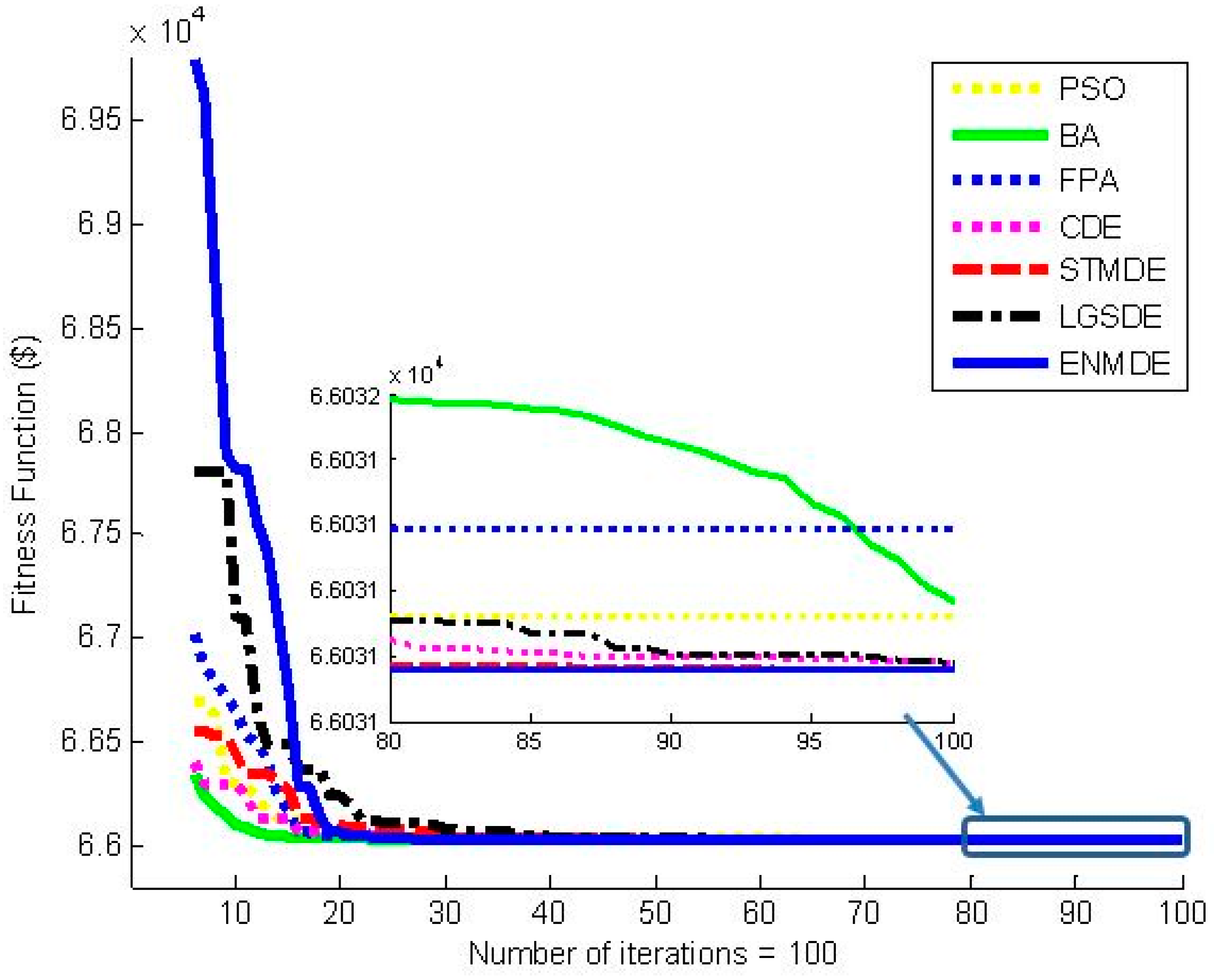
On the other hand, when comparing the proposed ENMDE with RCGA [14], BA, PSO, and FPA, the best cost from ENMDE was lower than that for RCGA [14], BA, PSO, and FPA by $0.2426, $0.2096, $0.1622, and $0.4794, respectively. The lower cost indicates that ENMDE is more efficient than these methods in finding the best optimal solution. Furthermore, ENMDE used 2000, corresponding to an execution time of 0.66 s, while RCGA employed 5000m corresponding to 21.64 s. These values from the proposed method and the others are equal and approximately equal. 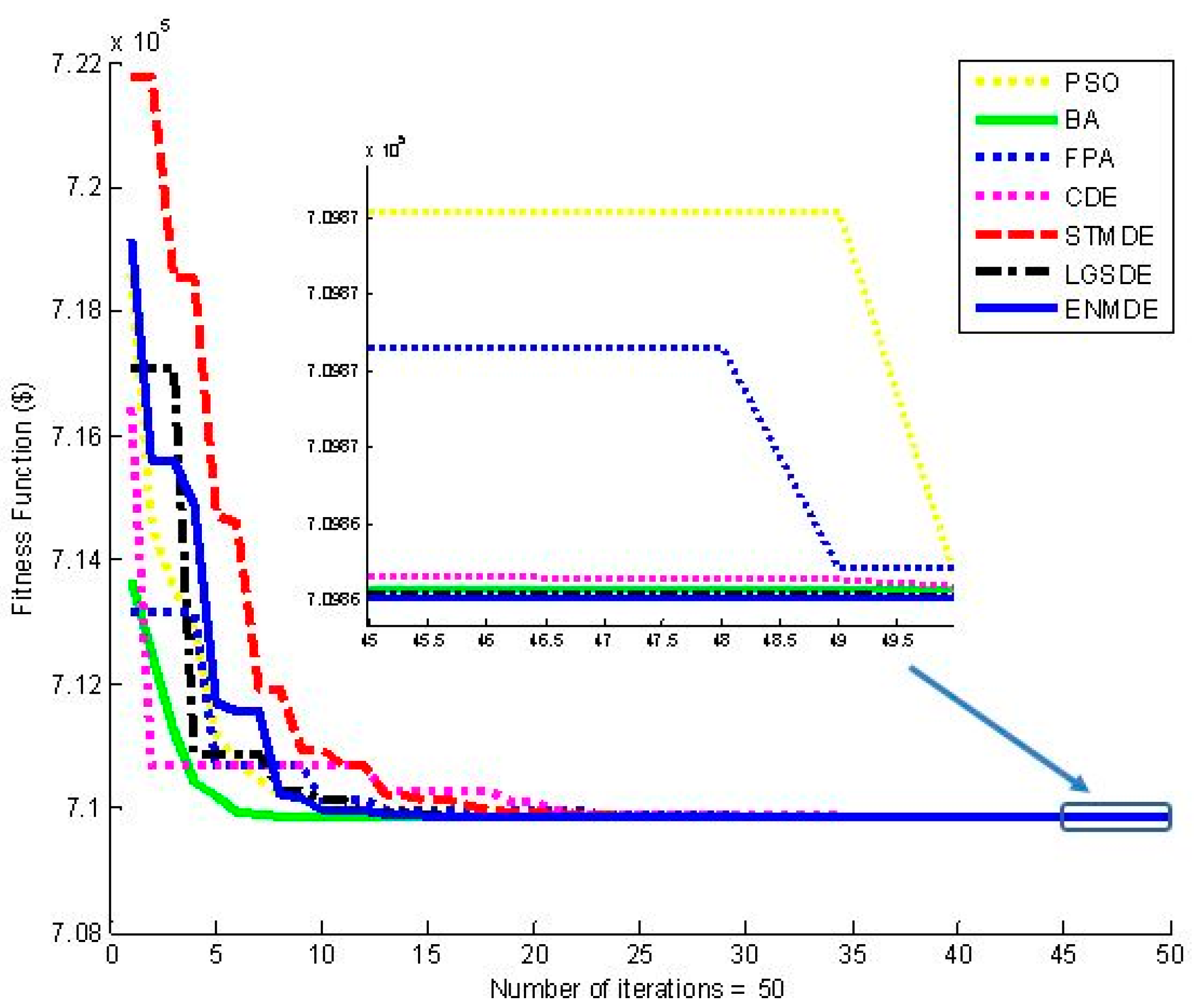The best fitness convergence characteristics obtained by these implemented methods, depicted in Figure 1, indicate that other methods tend to converge to local optimal solutions faster than the proposed ENMDE from the first iteration to the twentieth iteration, but these methods did not improve their fitness much from the eightieth to the last iteration. These methods are trapped into a local optimum and the jump out of the local zone was not carried out. It was clear that the search ability of the proposed ENMDE always improved when the iteration was increased. Consequently, it can be concluded that ENMDE is very effective for the study case of Problem 1.

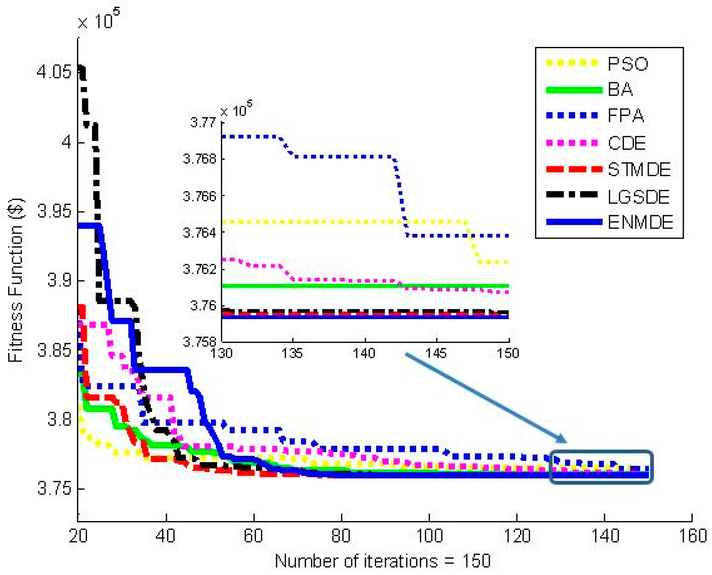
The result obtained by the four DE variants and other methods for study case two are reported in

Table 3. Result comparison for study case two.

Method	Np	Gmax	TNFES	Min. Cost ($)	Mean Cost ($)	Worst Cost ($)	Std. Dev. ($)	CPU Time (s)
Newton [6]	-	-	-	377,374.67	-	-	-	-
HNN [6]	-	-	-	377,554.94	-	-	-	-
HLN [15]	1	631	631	375,933.68	-	-	-	1.26
ALHN [15]	1	707	707	375,933.64	-	-	-	1.1
CSA [16]	100	1000	200,000	375,960.58	376,190.96	376,408.80	176.633	12.1
CSA [17]	50	5000	500,000	376,114.73	376,547.50	377,211.26	274.463	30.29
MCSA [17]	12	3000	72,000	375,990.46	376,060.43	376,167.66	40.997	7.9
BA	50	150	7500	376,104.35	382,443.8	415,403.5	8697.25	2
PSO	50	150	7500	376,226.96	377,166.4	380,492.3	726.12	2.05
FPA	50	150	7500	376,380.83	377,830.03	378,733.11	464.13	1.98
CDE	50	150	7500	376,070.25	376,542.94	377,609.57	434.65	2.38
STMDE	50	150	7500	375,951.86	376,119.84	377,152.44	265.34	2.16
LGSDE	50	150	7500	375,965.55	376,048.86	376,467.66	123.74	2.06
ENMDE	50	150	7500	375,933.71	375,958.45	376,158.14	48.16	2.08

. Similar to the results yielded for case one, the two proposed techniques have a significant impact on the performance of DE since the lowest cost, mean cost, highest cost, and standard deviation cost for STMDE and LGSDE are better than those for CDE. In particular, all the costs from the proposed ENMDE are the lowest values when compared to those from CDE, STMDE, LGSDE, BA, PSO, and FPA. The best cost for ENMDE is lower than that for CDE, STMDE, LGSDE, BA, PSO, and FPA by $136.54, $18.76, $31.84, $170.64, $293.25, and $447.12, respectively. 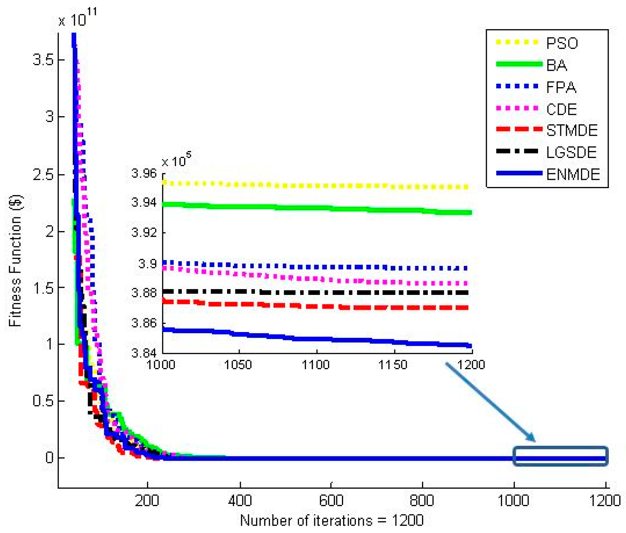The convergence characteristics shown in Figure 2 indicate that the other methods search very well at the beginning of the search process from the first iterations to the forty-fifth iteration, because their fitness functions were much lower than those of the proposed ENMDE. However, at the end of the search, from the 130th iteration to the last iteration, their fitness functions were much higher than those of the proposed ENMDE. Clearly, there are similarities between this scenario and scenario in case 1.

Compared to the others, the proposed ENMDE reveals its strongly highlighted search ability once its best cost is less than that of nearly all methods except HLN and ALHN in [15]. The best cost for ENMDE is slightly higher than HLN and ALHN, by $0.03 and $0.06, respectively; while the cost for ENMDE is much lower than others, such as $1621.23 compared to HNN, $1440.96 compared to the Newton method, $26.87 compared to CSA [16], $181.03 compared to CSA [17], and $56.76 compared to MCSA [17]. Furthermore, the TNFES for the proposed ENMDE is 7500; whilst that for CSA [16], and CSA and MCSA [17] were 200,000, 500,000, and 72,000, respectively. With respect to the execution time, HLN and ALHN still perform best, with the fastest times. However, as pointed out in the introduction, the two methods suffer from a large limitation for the application to a large number of constraints and problems with non-convex objective functions. Overall, it can be concluded that the proposed ENMDE is very efficient for study case two. The optimal solutions obtained by ENMDE for the two cases are given in Appendix A.

5.1.2 Study Cases 3 and 4 with Valve Point Loading Effects

In this section, a demonstration is implemented for two hydrothermal systems with a non-convex fuel cost function, for thermal units where the valve point loading effects of thermal generators are considered [8]. Study case three, including two hydropower plants and two thermal plants scheduled in three eight-hour subintervals, and study case four, including two hydropower plants and four thermal plants scheduled in four twelve-hour subintervals, are used to verify the performance of the proposed ENMDE method. The compared information reported in

Table 4. Result comparison for study case three.

Method	Np	Gmax	TNFES	Min. Cost ($)	Mean Cost ($)	Worst Cost ($)	Std. Dev. ($)	CPU Time (s)
AIS [8]	50	100	10,000	66,117	-	-	-	53.43
EP [8]	100	100	10,000	66,198	-	-	-	75.48
PSO [8]	100	100	10,000	66,166	-	-	-	71.62
DE [8]	100	100	10,000	66,121	-	-	-	60.76
CSA [16]	50	1500	150,000	66,115.45	66,133.86	66,158.10	18.54	6.7
CSA [17]	50	5000	500,000	66,115.59	66,126.92	66,147.82	13.25	23.1
MCSA [17]	12	3000	72,000	66,115.45	66,116.83	66,128.11	2.96	6.6
BA	50	70	3500	66,163.87	66,843.53	68,839.55	557.47	0.87
PSO	50	70	3500	66,163.34	66,286.54	66,308.19	62.09	0.76
FPA	50	70	3500	66,157.992	66,228.48	66,303.14	28.11	0.79
CDE	50	70	3500	66,122.11	66,247.88	66,310.91	33.64	1.02
STMDE	50	70	3500	66,116.66	66,164.84	66,245.37	31.81	0.95
LGSDE	50	70	3500	66,118.01	66,236.09	66,315.58	32.67	0.94
ENMDE	50	70	3500	66,115.44	66,183.25	66,204.15	20.82	0.96

for case three and in

Table 5. Result comparison for study case four.

Method	Np	Gmax	TNFES	Min. Cost ($)	Mean Cost ($)	Worst Cost ($)	Std. Dev. ($)	CPU Time (s)
AIS [8]	50	200	20,000	93,950.00	-	-	-	59.14
EP [8]	100	200	20,000	94,250.00	-	-	-	67.82
PSO [8]	100	200	20,000	94,126.00	-	-	-	80.37
DE [8]	100	200	20,000	94,094.00	-	-	-	83.54
CSA [16]	100	1500	300,000	92,725.13	92,779.32	92,934.77	56.324	18.6
CSA [17]	50	7000	700,000	92,767.09	92,870.80	93,132.55	99.0503	41.2
MCSA [17]	12	5000	120,000	92,741.90	92,836.66	92,938.54	47.7365	13.3
BA	40	500	20,000	93,966.13	127,220.60	166,755.10	20,067.30	4.5
PSO	40	500	20,000	93,956.40	96,071.21	101,067.38	1463.57	4.6
FPA	40	500	20,000	93,571.96	96,131.71	100,445.03	1540.93	4.1
CDE	40	500	20,000	93,214.38	96,008.15	120,163.40	1218.37	6.0
STMDE	40	500	20,000	92,782.03	94,091.11	100,041.66	960.81	5.6
LGSDE	40	500	20,000	92,780.07	95,972.80	106,527.11	2980.97	5.44
ENMDE	40	500	20,000	92,723.96	93,341.06	95,677.89	367.138	5.5

for case four includes fuel costs, standard deviation, and computation time in addition to the population size, the maximum number of iterations and the total number of fitness evaluations. As seen from TNFES in Table 4, the proposed ENMDE has the same value as the other implemented methods, such as BA, FPA, and DE variants, but the proposed ENMDE has much lower values than the other ones. In fact, the proposed ENMDE used 3500 fitness evaluations, while AIS, EP, PSO, and DE in [8] used 10,000 fitness evaluations, especially CSA in [16]; CSA and MCSA in [17] used 150,000, 500,000, and 72,000 fitness evaluations, respectively. A similar scenario can be also seen in Table 5, since the proposed ENMDE is in the group with the lowest TNFES of 20,000 fitness evaluations, while other methods used a very high number, such as CSA [16] with 300,000 fitness evaluations, CSA [17] with 700,000 fitness evaluations, and MCSA [17] with 120,000 fitness evaluations. Comparing the best cost for case three and case four, the proposed ENMDE has a much lower cost than several methods with the same TNFES and have a slightly lower cost than several methods with a much higher TNFES. For case three, the cost obtained by ENMDE was less than BA and FPA by $48.43 and $42.552, respectively. Equally, ENMDE has a much lower cost than AIS, EP, PSO, and DE, being $1.56, $82.56, $50.56, and $5.56 lower, respectively. ENMDE has a slightly lower cost than CSA [16] and CSA and MCSA [17], being $0.01, $0.15 and $0.01 lower, respectively. For case four, the cost obtained by ENMDE was $1242.17 and $848 lower than BA and FPA, respectively; $1226.04, $1526.04, $1402.04, and $1370.04 lower than AIS, EP, PSO, and DE [8], respectively; and $1.17, $43.13, and $17.94 lower than CSA [16] and CSA and MCSA [17], respectively. Similarly, the costs of the proposed ENMDE are also lower than CDE, STMDE and LGSDE. 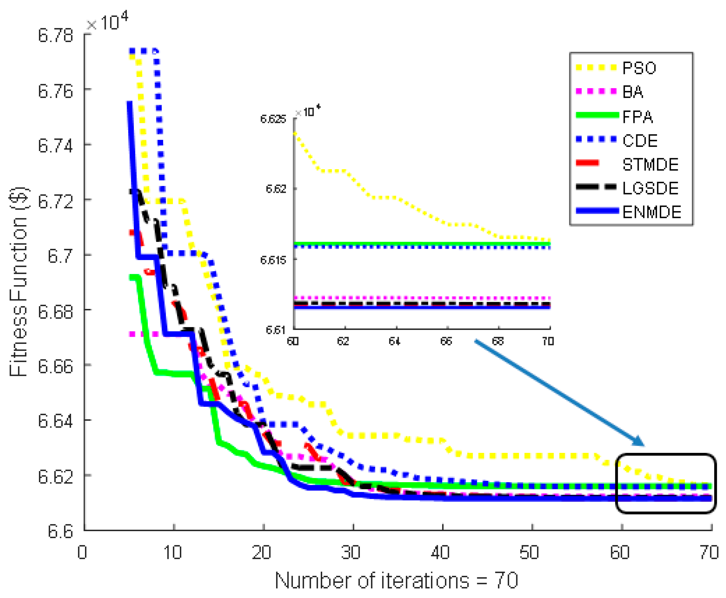Figure 3 and Figure 4 also show the better performance of the proposed ENMDE compared to other methods implemented in this paper. For the two cases with valve point loading effects, the application of HLN and ALHN in [15] could not be performed. Therefore, there was no evaluation of their performance. In summary, the proposed ENMDE is very efficient compared to other methods for solving study cases three and four with a non-convex fuel cost function. The optimal solutions obtained by ENMDE are given in the Appendix A.

5.2. The Second Problem with Reservoir Volume Constraints

In Section 5.1, a big effort was made to clarify the superiority of the proposed ENMDE over other algorithms, including conventional deterministic algorithms, original meta-heuristic algorithms and improved versions of original meta-heuristic algorithms, especially three other DE variants. In this section, the proposed ENMDE is tested on two other hydrothermal systems constrained by the reservoir volume, such as initial volume, end volume, and the limits on the volumes. The first system, called study case five, consists of one hydropower plant and one thermal plant, neglecting the valve point loading effects from [2]. The second system, consisting of four hydro units and four thermal units considering valve point loading effects, is called study case six and is modified from study case five [33].

5.2.1. Study Case 5 without Valve Point Loading Effects

The detailed results obtained by CDE, STMDE, LGSDE, ENMDE, and three additional methods, consisting of PSO, BA, and FPA, are shown in

Table 6. Comparison of the best results obtained by the implemented methods for study case five.

Method	Best Cost ($)	Mean Cost ($)	Worst Cost ($)	Std. Dev. ($)	CPU Time (s)
BA	709,862.2544	712,753.522	725,323.96	3559.16	0.14
PSO	709,862.5034	710,794.074	713,313.23	675.10	0.12
FPA	709,862.8147	710,498.097	717,063.51	1559.40	0.12
CDE	709,862.3718	710,142.287	713,592.06	639.58	0.15
STMDE	709,862.0788	710,480.001	712,168.02	450.16	0.13
LGSDE	709,862.1934	710,685.688	716,829.45	1171.40	0.14
ENMDE	709,862.0490	709,862.192	709,865.00	0.392	0.14

. The fitness convergence characteristics from the second iteration onwards yielded by these methods are depicted in Figure 5. As seen from the Table 6 and Figure 5, the proposed ENMDE obtained the best minimum, average, maximum, and standard deviation cost and the fastest convergence compared to other methods. The performance of the proposed ENMDE method continued to compete with other methods and is presented in

Table 7. Result comparisons for study case five.

Method	Best Cost ($)	Np	Gmax	TNFES	CPU Time (s)
GS [2]	709,877.38	-	-	-	-
SA [18]	709,874.36	-	200	-	901
GA [19]	709,863.56	30	300	9000	-
EP [19]	709,862.06	30	300	9000	8
EP [20]	709,863.29	50	400	20,000	2640
EP [23]	709,862.05	60	500	30,000	159.18
FEP [23]	709,862.05	60	300	18,000	101.4
IFEP [23]	709,862.05	60	150	9000	59.7
RIFEP [28]	709,862.05	-	300	-	-
CS [31]	709,862.05	30	70	2100	4.54
CSA-Lévy [33]	709,862.0489	30	400	24,000	0.26
CSA-Cauchy [33]	709,862.0489	30	400	24,000	0.28
CSA-Gauss [33]	709,862.0489	30	400	24,000	0.3
ORCSA-Lévy [34]	709,862.048	10	300	6000	0.18
ORCSA-Cauchy [34]	709,862.048	10	300	6000	0.18
ENMDE	709,862.049	20	50	1000	0.14

. The best cost comparison reveals that the proposed ENMDE could find a high quality solution, which was as good as that of all methods excluding GS [2], SA [18], GA [19], and EP [20], the costs of which were much higher. Although the best cost cannot lead to a superiority of the proposed ENMDE over some methods, the TNFES value that the ENMDE used was much lower than all methods. In fact, ENMDE used only 1000 fitness evaluations, while the others used from 2100 to 24,000 fitness evaluations. This large difference justified the fastest execution time of the proposed ENMDE of 0.14 s, while other methods (excluding the CSA methods in the studies [33,34]) required from 4.54 s (CS [31]) to 901 seconds (SA [18]). Thus, it can be concluded that ENMDE is very efficient for study case five. The optimal solutions obtained by ENMDE are provided in the Appendix A.

5.2.2. Study Case 6 with Valve Point Loading Effects of Thermal Units

In order to clarify the performance of the proposed ENMDE, the largest system with four hydro units and four thermal units scheduled in six twelve hour subintervals considering the valve point loading effects was used. The results obtained by the CDE, STMDE, LGSDE, and ENMDE and the three additional methods, consisting of PSO, BA, and FPA accompanied by N_p, G_max and TNFES are compared and presented in

Table 8. Result comparisons of the best results from differential evolution (DE) variants for study case six.

Method	Np	Gmax	TNFES	Best Cost ($)	Mean Cost ($)	Worst Cost ($)	Std. Dev. ($)	CPU Time (s)
CSA-Lévy [33]	50	3500	350,000	387,725.60	396,692.50	468,641.10	11,167.30	47.6
CSA-Cauchy [33]	50	3500	350,000	388,887.70	394,450.20	409,167.80	4415.70	49.9
CSA-Gauss [33]	50	3500	350,000	389,213.50	400,034.09	495,151.00	22,239.40	48.3
BA	50	1200	60,000	393,381.70	454,354.80	499,789.6	31,350.40	35.6
PSO	50	1200	60,000	395,099.6	449,470.10	495,411.80	29,556.60	33.4
FPA	50	1200	60,000	389,656.20	429,731.60	466,392.8	23,993.30	34.8
CDE	50	1200	60,000	388,661.80	423,132.60	492,816.40	21,599.50	36.7
STMDE	50	1200	60,000	386,975.91	401,745.60	408,083.10	3026.60	34.6
LGSDE	50	1200	60,000	388,018.90	405,461.00	419,744.80	7573.20	34.5
ENMDE	50	1200	60,000	384,518.09	395,114.20	405,582.30	2766.90	34.4

. The comparison of all the shown values implies that the proposed ENMDE is the most efficient method with the best costs and the lowest TNFES value. In fact, ENMDE, other DE variants, and PSO, BA and FPA used the same TNFES, with only 60,000, while the values for the CSA variants was very high and equal to 350,000. In addition, the best cost from the proposed ENMDE was respectively less than that of CSA-Lévy, CSA-Cauchy, CSA-Gauss, CDE, STMDE, LGSDE, BA, PSO, and FPA by $3207.5, $4369.6, $4695.4, $4143.7, $2457.9, $3500.8, $8863.6, $10,581.5, and $5138.1, respectively. 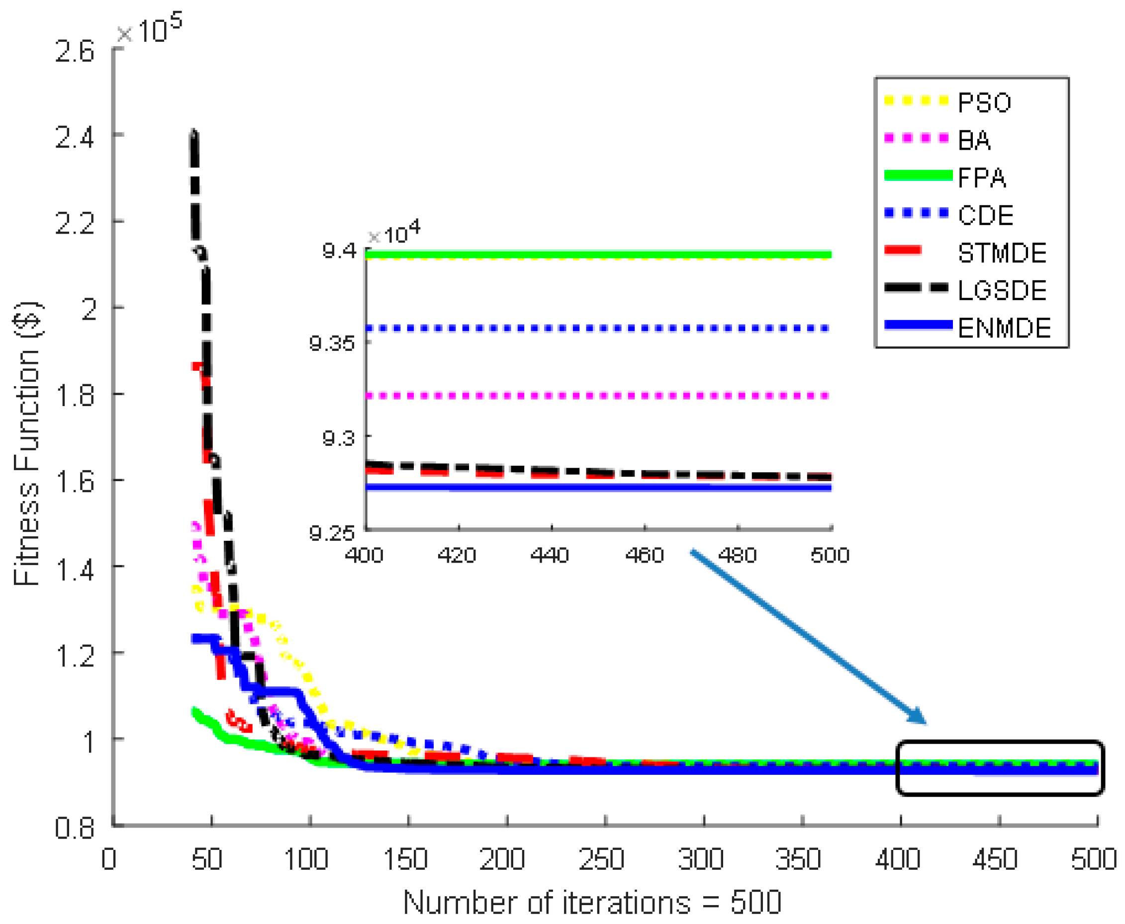Figure 6 indicates the faster convergence of the proposed ENMDE than other DE variants, namely BA, PSO, and FPA. In summary, the proposed ENMDE can both obtain a better optimal solution and has faster convergence than all methods for the study case 5 with reservoir volume constraints and a non-convex fuel cost function. The optimal solutions obtained by ENMDE are given in Appendix A.

5.3. Discussion of the Performance of the Proposed Method

In this work, we employed six benchmark systems and tried to demonstrate the effectiveness and robustness of the proposed method on the systems by adding a non-convex fuel cost function, increasing the number of power plants and changing the complex of set of constraints. We applied two different problems, where the first problem considers the constraint of available water and ignores the constraints related to reservoir volumes, such as reservoir volume limitation, the initial volume of reservoirs and the end volume of reservoirs, while the second problem ignores the constraints of available water but takes all constraints regarding the reservoir volume into account. For the challenge of searching for the global optimum solutions or near-global-optimum solutions, the valve point loading effects, which are represented as a non-convex fuel cost function form, were considered in study cases three and four in problem one and in study case six in problem two. Besides, the scale of the study cases also increased, such as the four power plants for cases one, two and three, six power plants for case four of problem one, two power plants for case five, and eight power plants for case six of problem two.

As observed from cost comparisons, the improvement of fuel cost obtained by the proposed method compared to the other methods is different for different study cases and the improvement is only significant for study case six. For a better performance evaluation between the proposed method and other methods, we supplemented cost saving and cost improvement in

Table 9. Cost saving and cost improvement of the proposed method compared to others for study cases one and two.

Study Case 1			Study Case 2
Method	Cost Saving ($)	Cost Improvement (%)	Method	Cost Saving ($)	Cost Improvement (%)
RCGA [14]	0.243	0.00037	Newton [6]	1440.96	0.382
BA	0.210	0.00032	HNN [6]	1621.23	0.429
PSO	0.163	0.00025	HLN [15]	−0.03	0.000
FPA	0.480	0.00073	ALHN [15]	−0.07	0.000
CDE	0.021	0.00003	CSA [16]	26.87	0.007
STMDE	0.002	0.00000	CSA [17]	181.02	0.048
LGSDE	0.019	0.00003	MCSA [17]	56.75	0.015
			BA	170.64	0.045
			PSO	293.25	0.078
			FPA	447.12	0.119
			CDE	136.54	0.036
			STMDE	18.15	0.005
			LGSDE	31.84	0.008

,

Table 10. Cost saving and cost improvement of the proposed method compared to others for study cases three and four.

Method	Study Case 3		Study Case 4
	Cost Saving ($)	Cost Improvement (%)	Cost Saving ($)	Cost Improvement (%)
AIS [8]	1.56	0.0024	1226.04	1.305
EP [8]	82.56	0.1247	1526.04	1.619
PSO [8]	50.56	0.0764	1402.04	1.49
DE [8]	5.56	0.0084	1370.04	1.456
CSA [16]	0.01	0.0000	1.17	0.001
CSA [17]	0.15	0.0002	43.13	0.046
MCSA [17]	0.01	0.0000	17.94	0.019
BA	48.43	0.0732	1242.17	1.322
PSO	47.90	0.0724	1232.44	1.31
FPA	42.55	0.0643	848	0.906
CDE	6.67	0.0101	490.42	0.526121
STMDE	1.22	0.0018	58.07	0.063
LGSDE	2.57	0.0039	56.11	0.06

and

Table 11. Cost saving and cost improvement of the proposed method compared to others for study cases five and six.

Study Case 5			Study Case 6
Method	Cost Saving ($)	Cost Improvement (%)	Method	Cost Saving ($)	Cost Improvement (%)
GS [2]	15.33	0.0022	CSA-Lévy [33]	3207.51	0.827
SA [18]	12.31	0.0017	CSA-Cauchy [33]	4369.61	1.124
GA [19]	1.51	0.0002	CSA-Gauss [33]	4695.41	1.206
EP [19]	0.01	0.0000	BA	8863.61	2.253
EP [20]	1.24	0.0002	PSO	10,581.51	2.678
EP [23]	0.00	0	FPA	5138.11	1.319
FEP [23]	0.00	0	CDE	4143.71	1.066
IFEP [23]	0.00	0	STMDE	2457.82	0.635
RIFEP [28]	0.00	0	LGSDE	3500.81	0.902
CS [31]	0.00	0
CSA-Lévy [33]	0.00	0
CSA-Cauchy [33]	0.00	0
CSA-Gauss [33]	0.00	0
ORCSA-Lévy [34]	0.00	0
ORCSA-Cauchy [34]	0.00	0

, in which cost saving in dollars and cost improvement in percent were calculated using Equation (37) and (38). Cost saving is the cost reduction of the proposed method compared to other methods, while cost improvement is the improvement of the proposed method over compared methods.

$$\mathrm{Cost}\mathrm{saving}(\$)=\mathrm{Cost}\mathrm{of}\mathrm{a}\mathrm{compared}\mathrm{method}(\$)-\mathrm{Cost}\mathrm{of}\mathrm{the}\mathrm{proposed}\mathrm{method}(\$)$$

(37)

$$\mathrm{Cost}\mathrm{improvement}(\%)=\frac{\mathrm{Cost}\mathrm{saving}}{\mathrm{Cost}\mathrm{of}\mathrm{a}\mathrm{compared}\mathrm{method}}\times 100\%$$

(38)

The cost improvement reported in these tables indicates that the highest cost improvements for cases 1–6 were 0.00073%, 0.382%, 0.1247%, 1.619%, 0.0017%, and 2.678%, respectively; while the lowest cost improvement for cases 1–5 was approximately 0%, excluding case six with a cost improvement of 0.635%. The difference among such numbers can be understood if the scale and the complex of the systems in Table 1 are analyzed. It can be seen that the cost improvement for case two (0.382%) was higher than that for case one (0.00073%), because case two considers a scheduled period of two days with 48 hours, while case one considers the period of one day only. Similarly, the cost improvement for case four (1.619%) and case six (2.678%) are much higher than those for case three (0.1247%) and case five (0.0017%), respectively. The number of power plants for case three is four units and the scheduled period for case three is one day; while those for case four are six power plants and two days. Similarly, those for case five are two power plants and three days, but those for case six are eight power plants and three days. The analysis can send a message that a large-scale system can lead to better cost improvement. Besides, the cost improvement for the cases considering complex objective functions with VPLES is also better than the cases neglecting such VPLES. For instance, the improvement in case three with VPLES is 0.1247%, while that for case one without VPLES is 0.00073%, although these two cases consider the same number of power plants and the same scheduled period. Due to both the higher number of power plants and the much more complicated objective function with VPLES, the cost improvement for case four is 1.619%, that for case six is 2.678%, and that for case 2 is 0.382%.

With respect to the performance comparison, we have stated that the proposed method was more effective and robust than the other methods based on four comparison criteria consisting of the minimum fuel cost comparison, the standard deviation comparison, computational time comparison, and TNFES comparison. Among the four comparisons, the minimum fuel cost comparison reflects the quality of the optimal solutions and the standard deviation comparison points out the robustness of the methods, while the computational time and TNFES comparisons reflect the convergence speed. The proposed method obtained insignificantly lower fuel costs than most methods for cases 1–3 and five but for case four and case six, the lower cost is relatively high. The greater lower cost for cases four and six resulted in the evaluation that the optimal solutions for the proposed method for cases four and six are of higher quality than those of other methods. The slightly lower cost for cases 1–3 and five cannot result in the same conclusion as for cases four and six, but it can lead to the evaluation that these compared methods have not converged to the global optimum or the near-global optimum. In fact, these methods need more iterations to find the same global optimal solutions. Furthermore, the computational time and the TNFES value from the proposed method are also smaller or approximate to those from other methods, excluding deterministic methods such as ALHN and HLN.

6. Conclusions

This paper presents the application of the proposed ENMDE method to solving two different STHTS problems with available water constraints and reservoir volume constraints, in addition to the valve point loading effects of thermal units. The proposed ENMDE with two new proposed techniques, including self-tuned mutation and leading group selection, has effective search abilities, such as fast convergence to the optimal solution, a low total number of fitness evaluations and few control parameters. The superiority of the proposed method over the conventional DE is not only the obtained results in terms of optimal solutions, but also the reduction of computation, such as neglecting crossover operations and cutting the crossover factor. Compared to other existing methods, the proposed ENMDE is also more effective in terms of a better quality of solutions, lower total number of fitness evaluations, and faster execution time. From these advantages, it should be concluded that the proposed ENMDE is very efficient for solving the two HTS problems.

References

1. El-Hawary, M.E.; Landrigan, J.K. Optimum operation of fixed-head hydro-thermal electric power systems: Powell’s hybrid method versus Newton-Raphson method. IEEE Trans. Power Appar. Syst. 1982, PAS-101, 547–554. [Google Scholar] [CrossRef]
2. Wood, A.J.; Wollenberg, B.F. Power Generation, Operation and Control, 2nd ed.; John Wiley & Sons: New York, NY, USA, 1996. [Google Scholar]
3. Zaghlool, M.F.; Trutt, F.C. Efficient methods for optimal scheduling of fixed head hydrothermal power systems. IEEE Trans. Power Syst. 1988, 3, 24–30. [Google Scholar] [CrossRef]
4. Rashid, A.H.A.; Nor, K.M. An efficient method for optimal scheduling of fixed head hydro and thermal plants. IEEE Trans. Power Syst. 1991, 6, 632–636. [Google Scholar] [CrossRef]
5. Salam, M.S.; Nor, K.M.; Hamdam, A.R. Hydrothermal scheduling based Lagrangian relaxation approach to hydrothermal coordination. IEEE Trans. Power Syst. 1998, 13, 226–235. [Google Scholar] [CrossRef]
6. Basu, M. Hopfield neural networks for optimal scheduling of fixed head hydrothermal power systems. Electr. Power Syst. Res. 2003, 64, 11–15. [Google Scholar] [CrossRef]
7. Sharma, A.K. Short Term Hydrothermal Scheduling Using Evolutionary Programming. Master’s Thesis, Thapar University, Patiala, India, 2009. [Google Scholar]
8. Basu, M. Artificial immune system for fixed head hydrothermal power system. Energy 2011, 36, 606–612. [Google Scholar] [CrossRef]
9. Farhat, I.A.; El-Hawary, M.E. Fixed-head hydro-thermal scheduling using a modified bacterial foraging algorithm. In Proceedings of the Electric Power and Energy Conference (EPEC), Halifax, NS, Canada, 25–27 August 2010. [Google Scholar]
10. Sasikala, J.; Ramaswamy, M. Optimal gamma based fixed head hydrothermal scheduling using genetic algorithm. Expert Syst. Appl. 2010, 37, 3352–3357. [Google Scholar] [CrossRef]
11. Murali, M.; Kumari, M.S.; Sydulu, M. Short-range fixed head hydrothermal scheduling using fast genetic algorithm. In Proceedings of the 7th IEEE Conference on Industrial Electronics and Applications (ICIEA), Singapore, 18–20 July 2012. [Google Scholar]
12. Narang, N.; Dhillon, J.S.; Kothari, D.P. Scheduling short-term hydrothermal generation using predator prey optimization technique. Appl. Soft Comput. 2014, 21, 298–308. [Google Scholar] [CrossRef]
13. Chiang, C.L. Optimal economic emission dispatch of hydrothermal power systems. Int. J. Electr. Power Energy Syst. 2007, 29, 462–469. [Google Scholar] [CrossRef]
14. Basu, M. Economic environmental dispatch of fixed head hydrothermal power systems using nondominated sorting genetic algorithm-II. Appl. Soft Comput. 2011, 11, 3046–3055. [Google Scholar] [CrossRef]
15. Dieu, V.N.; Ongsakul, W. Hopfield Lagrange for short-term hydrothermal scheduling. In Proceedings of the IEEE Russia Power Tech, St. Petersburg, Russia, 27–30 June 2005. [Google Scholar]
16. Nguyen, T.T.; Vo, D.N.; Truong, A.V. Cuckoo search algorithm for short-term hydrothermal scheduling. Appl. Energy 2014, 132, 276–287. [Google Scholar] [CrossRef]
17. Nguyen, T.T.; Vo, D.N. Modified cuckoo search algorithm for short-term hydrothermal scheduling. Int. J. Electr. Power Energy Syst. 2015, 65, 271–281. [Google Scholar] [CrossRef]
18. Wong, K.P.; Wong, Y.W. Short-term hydrothermal scheduling Part. I. Simulated annealing approach. IEE Proc. Gener. Trans. Distrib. 1994, 141, 497–501. [Google Scholar] [CrossRef]
19. Yang, P.C.; Yang, H.T.; Huang, C.L. Scheduling short-term hydrothermal generation using evolutionary programming techniques. IEE Proc. Gener. Trans. Distrib. 1996, 143, 371–376. [Google Scholar] [CrossRef]
20. Hota, P.K.; Chakrabarti, R.; Chattopadhyay, P.K. Short-term hydrothermal scheduling through evolutionary programming technique. Electr. Power Syst. Res. 1999, 52, 189–196. [Google Scholar] [CrossRef]
21. Sinha, N.; Chakrabarti, R.; Chattopadhyay, P.K. Fast evolutionary programming techniques for short-term hydrothermal scheduling. IEEE Trans. Power Syst. 2003, 18, 214–220. [Google Scholar] [CrossRef]
22. Chang, H.C.; Chen, P.H. Hydrothermal generation scheduling package: A genetic based approach. IEE Proc. Gener. Trans. Distrib. 1998, 145, 451–457. [Google Scholar] [CrossRef]
23. Sinha, N.; Chakrabarti, R.; Chattopadhyay, P.K. Fast evolutionary programming techniques for short-term hydrothermal scheduling. Electr. Power Syst. Res. 2003, 66, 97–103. [Google Scholar] [CrossRef]
24. Nallasivan, C.; Suman, D.S.; Henry, J.; Ravichandran, S. A novel approach for short-term hydrothermal scheduling using hybrid technique. In Proceedings of the IEEE Power India Conference, New Delhi, India, 10–12 April 2006. [Google Scholar]
25. Samudi, C.; Das, G.P.; Ojha, P.C.; Sreeni, T.S.; Cherian, S. Hydro thermal scheduling using particle swarm optimization. In Proceedings of the Transmission and Distribution Conference and Exposition, Chicago, IL, USA, 21–24 April 2008. [Google Scholar]
26. Farhat, I.A.; El-Hawary, M.E. Short-term hydro-thermal scheduling using an improved bacterial foraging algorithm. In Proceedings of the IEEE Electrical Power & Energy Conference (EPEC), Montreal, QC, Canada, 22–23 October 2009. [Google Scholar]
27. Thakur, S.; Boonchay, C.; Ongsakul, W. Optimal Hydrothermal Generation Scheduling using Self-Organizing Hierarchical PSO. In Proceedings of the IEEE Power and Energy Society General Meeting, Providence, RI, USA, 25–29 July 2010. [Google Scholar]
28. Türkay, B.; Mecitoğlu, F.; Baran, S. Application of a fast evolutionary algorithm to short-term hydro-thermal generation scheduling. Energy Sources Part B Econ. Plan. Policy 2011, 6, 395–405. [Google Scholar] [CrossRef]
29. Padmini, S.; Rajan, C.C.A. Improved PSO for Short Term Hydrothermal Scheduling. In Proceedings of the International Conference on Sustainable Energy and Intelligent Systems (SEISCON 2011), Chennai, India, 20–22 July 2011. [Google Scholar]
30. Padmini, S.; Rajan, C.C.A.; Murthy, P. Application of improved PSO technique for short term hydrothermal generation scheduling of power system. In International Conference on Swarm, Evolutionary, and Memetic Computing; Springer: Berlin/Heidelberg, Germany, 2011. [Google Scholar]
31. Swain, R.K.; Barisal, A.K.; Hota, P.K.; Chakrabarti, R. Short-term hydrothermal scheduling using clonal selection algorithm. Int. J. Electr. Power Energy Syst. 2011, 33, 647–656. [Google Scholar] [CrossRef]
32. Fakhar, M.S.; Kashif, S.A.R.; Saqib, M.A.; ul Hassan, T. Non cascaded short-term hydro-thermal scheduling using fully-informed particle swarm optimization. Int. J. Electr. Power Energy Syst. 2015, 73, 983–990. [Google Scholar] [CrossRef]
33. Nguyen, T.T.; Vo, D.N.; Dinh, B.H. Cuckoo search algorithm using different distributions for short-term hydrothermal scheduling with reservoir volume constraint. Int. J. Electr. Eng. Inf. 2016, 8, 76. [Google Scholar] [CrossRef]
34. Nguyen, T.T.; Vo, D.N.; Ongsakul, W. One rank cuckoo search algorithm for short-term hydrothermal scheduling with reservoir constraint. In Proceedings of the IEEE Eindhoven PowerTech, Eindhoven, The Netherlands, 29 June–2 July 2015. [Google Scholar]
35. Storn, R.; Price, K. Differential evolution—A simple and efficient heuristic for global optimization over continuous spaces. J. Glob. Optim. 1997, 11, 341–359. [Google Scholar] [CrossRef]
36. Chang, C.F.; Wong, J.J.; Chiou, J.P.; Su, C.T. Robust searching hybrid differential evolution method for optimal reactive power planning in large-scale distribution systems. Electr. Power Syst. Res. 2007, 77, 430–437. [Google Scholar] [CrossRef]
37. Chiou, J.P. Variable scaling hybrid differential evolution for large-scale economic dispatch problems. Electr. Power Syst. Res. 2007, 77, 212–218. [Google Scholar] [CrossRef]
38. Varadarajan, M.; Swarup, K.S. Differential evolution approach for optimal reactive power dispatch. Appl. Soft Comput. 2008, 8, 1549–1561. [Google Scholar] [CrossRef]
39. Ho-Huu, V.; Nguyen-Thoi, T.; Nguyen-Thoi, M.H.; Le-Anh, L. An improved constrained differential evolution using discrete variables (D-ICDE) for layout optimization of truss structures. Expert Syst. Appl. 2015, 42, 7057–7069. [Google Scholar] [CrossRef]
40. Kamboj, V.K.; Bath, S.K.; Dhillon, J.S. Multiobjective multiarea unit commitment using hybrid differential evolution algorithm considering import/export and tie-line constraints. Neural Comput. Appl. 2017, 28, 3521–3536. [Google Scholar] [CrossRef]
41. Qin, A.K.; Huang, V.L.; Suganthan, P.N. Differential evolution algorithm with strategy adaptation for global numerical optimization. IEEE Trans. Evol. Comput. 2009, 13, 398–417. [Google Scholar] [CrossRef]
42. Padhye, N.; Bhardawaj, P.; Deb, K. Improving differential evolution through a unified approach. J. Glob. Optim. 2013, 55, 771. [Google Scholar] [CrossRef]
43. Prado, R.S.; Silva, R.C.P.; Neto, O.M.; Guimarães, F.G.; Sanches, D.S.; London, J.B.A.; Delbem, A.C. Differential evolution using ancestor tree for service restoration in power distribution systems. Appl. Soft Comput. 2014, 23, 498–508. [Google Scholar] [CrossRef] [Green Version]
44. Ho-Huu, V.; Nguyen-Thoi, T.; Vo-Duy, T.; Nguyen-Trang, T. An adaptive elitist differential evolution for optimization of truss structures with discrete design variables. Comput. Struct. 2016, 165, 59–75. [Google Scholar] [CrossRef]
45. Ishaque, K.; Salam, Z.; Mekhilef, S.; Shamsudin, A. Parameter extraction of solar photovoltaic modules using penalty-based differential evolution. Appl. Energy 2012, 99, 297–308. [Google Scholar] [CrossRef]
46. Glotić, A.; Zamuda, A. Short-term combined economic and emission hydrothermal optimization by surrogate differential evolution. Appl. Energy 2015, 141, 42–56. [Google Scholar] [CrossRef]
47. Das, S.; Abraham, A.; Chakraborty, U.K.; Konar, A. Differential evolution using a neighborhood-based mutation operator. IEEE Trans. Evol. Comput. 2009, 13, 526–553. [Google Scholar] [CrossRef]
48. Jia, G.; Wang, Y.; Cai, Z.; Jin, Y. An improved (μ+λ)-constrained differential evolution for constrained optimization. Inf. Sci. 2013, 222, 302–322. [Google Scholar] [CrossRef]
49. Yang, X.S. Nature-Inspired Optimization Algorithms; Elsevier: London, UK, 2014. [Google Scholar]
50. Wang, Y.; Cai, Z.; Zhang, Q. Differential evolution with composite trial vector generation strategies and control parameters. IEEE Trans. Evol. Comput. 2011, 15, 55–66. [Google Scholar] [CrossRef]
51. Kennedy, J.; Eberhart, R. Particle swarm optimization. In Proceedings of the IEEE International Conference on Neural Networks, Perth, WA, Australia, 27 November–1 December 1995. [Google Scholar]
52. Yang, X.S. A new metaheuristic bat-inspired algorithm. In Nature Inspired Cooperative Strategies for Optimization; Springer-Verlag: Berlin/Heidelberg, Germany, 2010. [Google Scholar]
53. Yang, X.S. Flower pollination algorithm for global optimization. In Unconventional Computation and Natural Computation: 11th International Conference on Unconventional Computing and Natural Computation (UCNC), Orléan, France, 3–7 September 2012; Springer-Verlag: Berlin/Heidelberg, Germany, 2012. [Google Scholar]
54. Mohamed, A.W.; Sabry, H.Z. Constrained optimization based on modified differential evolution algorithm. Inf. Sci. 2012, 194, 171–208. [Google Scholar] [CrossRef]
55. Mernik, M.; Liu, S.H.; Karaboga, D.; Črepinšek, M. On clarifying misconceptions when comparing variants of the artificial bee colony algorithm by offering a new implementation. Inf. Sci. 2015, 291, 115–127. [Google Scholar] [CrossRef]
56. Price, K.V. Differential evolution: A fast and simple numerical optimizer. In Proceedings of the Biennial Conference of the North American Fuzzy Information Processing Society, Berkeley, CA, USA, 19–22 June 1996. [Google Scholar]
Figure 1. Fitness convergence characteristics obtained for case one.
Energies 11 00540 g001
Figure 2. Fitness convergence characteristics obtained for case two.
Energies 11 00540 g002
Figure 3. Fitness convergence characteristics obtained for case three.
Energies 11 00540 g003
Figure 4. Fitness convergence characteristics obtained for case four.
Energies 11 00540 g004
Figure 5. Fitness convergence characteristics obtained for study case five.
Energies 11 00540 g005
Figure 6. Fitness convergence characteristics obtained for study case six.
Energies 11 00540 g006