Wind Predictions Upstream Wind Turbines from a LiDAR Database

ETSIAE (School of Aeronautics), Universidad Politécnica de Madrid, E-28040 Madrid, Spain
*
Author to whom correspondence should be addressed.
Energies 2018, 11(3), 543; https://doi.org/10.3390/en11030543
Submission received: 22 January 2018
/
Revised: 19 February 2018
/
Accepted: 22 February 2018
/
Published: 3 March 2018
(This article belongs to the Special Issue Data Science and Big Data in Energy Forecasting)
Abstract
:This article presents a new method to predict the wind velocity upstream a horizontal axis wind turbine from a set of light detection and ranging (LiDAR) measurements. The method uses higher order dynamic mode decomposition (HODMD) to construct a reduced order model (ROM) that can be extrapolated in space. LiDAR measurements have been carried out upstream a wind turbine at six different planes perpendicular to the wind turbine axis. This new HODMD-based ROM predicts with high accuracy the wind velocity during a timespan of 24 h in a plane of measurements that is more than 225 m far away from the wind turbine. Moreover, the technique introduced is general and obtained with an almost negligible computational cost. This fact makes it possible to extend its application to both vertical axis wind turbines and real-time operation.
1. Introduction
Light detection and ranging (LiDAR) [1,2] offers a method for the remote measurement of the line-of-sight component of wind speed, at distances between 10 and 200 m from the measurement device [3,4]. Measurements are based on detection of the Doppler shift for light backscattered from natural aerosols transported by the wind in the atmosphere. During the last two decades, the continuous wave (CW) version of the LiDAR system (see [1] for an overview of different LiDAR techniques) has been introduced in many industrial applications, especially, in the wind energy industry. Ground-based CW LiDAR systems have been accurately tested against cup anemometers in a meteorological mast [5,6], including the analysis of different sites with different terrain conditions [7] yielding excellent results in all cases. Moreover, the system has been used in offshore platforms at different wind conditions [8], again yielding excellent correlation with cup anemometer measurements up to heights of 160 m. In addition, it has been demonstrated that the LiDAR system is capable of detecting wind gusts [4,9] when the LiDAR transceiver is mounted on top of the nacelle of the wind turbine.
There are multiple applications of LiDAR technology in connection with the incoming wind characterization in wind turbines. For example, LiDAR is being used to replace meteorological masts in wind resource assessment [5,7]. Traditionally, resource assessment is performed using meteorological mast with sonic and cup anemometers of the same height of the wind turbine hub along a period of two years. However, the installation and operation of these masts in a two years cycle is fairly expensive [5] and the masts are limited to heights of 100–120 m approximately, while modern wind turbines hub height currently exceeds 130 m, a distance that is accessible to LiDAR.
Another application of LiDAR technology consists in using LiDAR wind speed measurements to improve the computation of the wind turbines power curve. The norm [10] defines the power curve measurement process and includes the installation of a meteorological mast between 2 and 4 wind turbine diameters (200–500 m) upstream of the wind turbine. Ground-based [11] and nacelle mounted [12] pulsed LiDAR have been used to improve the power curve measurement process replacing the use of meteorological masts. The use of CW LiDAR for this purpose is conditioned to the range limit of this technology (currently, 200 m).
One last example of application of LiDAR technology is active control of blade pitch [13]. The joint control of blades pitch, as well as the individual control of each blade pitch [14], have demonstrated the reduction of extreme loads, the reduction of emergency shutdowns, and the reduction of fatigue loads in wind turbines. The use of nacelle mounted LiDAR measurements of wind speed suggested by Mikkelsen et al. [4] allows for the use of feed-forward control algorithms [15,16]. These control systems have been tested with real data [17,18], demonstrating a 10–30% reduction of structural loads.
Higher order dynamic mode decomposition (HODMD) [19] is a recently introduced method that can be seen as a step further from standard dynamic mode decomposition (DMD) [20]. The additional ingredient from standard DMD consists in using delayed snapshots, meaning that HODMD synergically combines the advantages of standard DMD and Takens delayed embedding theorem [21]. HODMD is a suitable tool to analyze flow patterns and flow structures in highly complex flows, transient dynamics [22], noisy particle image velocimetry (PIV) data [23] or in cases in which the number of data collected are limited in space, but the dynamics is highly complex (quasi-periodic) in time [24].
HODMD provides a reduced order model (ROM) of the incoming wind flow based on a decomposition into spatio-temporal modes. This representation of the wind field is potentially useful for improving the performance of the LiDAR technology applications described above. For example, as it will be demonstrated in this paper, spatial HODMD modes provide an efficient method for spatial extrapolation of the wind field. Accurately extrapolating the LiDAR wind speed data could be used to extend the range of CW LiDAR measurements, allowing for the use of CW LiDAR in power curve calculation, as well as in characterizing the wind field up to blade tip height. In addition, spatial modes of the wind field could be used to improve the feed-forward control algorithms, reducing the parameter space to be modeled in the control algorithm. Finally, we can envisage the use of the HODMD spatio-temporal modes and frequencies in turbulent wind simulators for extreme and fatigue loads calculations.
This article is focused on demonstrating the modeling and spatial extrapolation capabilities of HODMD. This study is based on a data set collected by the company ZephIR LiDAR [25] during a 24 h timespan. Application of HODMD to the LiDAR data yields the main temporal frequencies and the associated spatial modes, which are used to extrapolate the wind field beyond the range of the LiDAR system. In other words, HODMD has been applied to a set of real LiDAR data collected during 24 h taken at 6 different locations upstream a horizontal axis wind turbine to construct a ROM. This model is then used to predict the evolution of the wind velocity during the same 24 h timespan at a new position beyond the range of LiDAR measurements. The computational cost for both constructing the ROM and predicting these measurements is negligible, making possible to easily update the model in real-time. Moreover, although the method has been tested in a horizontal axis wind tubine, it could also be used in vertical axis wind turbines, since this technique conserves the same features as HODMD: generalisation and robustness [19,22,23].
Regarding the organization of this article, the HODMD method is introduced first, in Section 2, and then illustrated in Section 3, where a toy model is considered that is free of noise. This section intends the reader to familiarize with the methodology to be used in following sections. Section 4 contains some details on the iterative HODMD method that is to be applied to the spatial extrapolation of LiDAR data. Section 5 is devoted to the application of the methodology to a database resulting from actual LiDAR wind measurements. Finally, the main conclusions are presented in Section 6.
2. Higher Order Dynamic Mode Decomposition
The main goal of HODMD is to express a set of instantaneous spatial data , to be called the snapshots, collected at K equispaced time instants, as an expansion in M spatio-temporal modes, in the following way:
Here, are the spatial modes, which are normalized to exhibit unit norm, will be called the mode amplitudes, and the temporal dynamics is characterized by the frequencies and growth rates . Retaining those spatio-temporal modes exhibiting the largest mode amplitudes will give a good approximation of the spatio-temporal behavior.
Let us briefly summarize the HODMD algorithm, which is described in full detail in [19]. As a previous step, a set of K time equispaced snapshots are collected in the following snapshot matrix:
where each vector is composed by the signal (e.g., spatial velocity distribution) at time . In fact, in the present application, the snapshots will contain the wind velocity at those points where the LiDAR measurements are performed. Then, the HODMD algorithm proceeds in two main steps:
- Step 1: Dimension reduction. The spatial dimension J (i.e., the number of planes of measurements in LiDAR experiments) of the original data set of snapshots is reduced by writing down the snapshots as linear combinations of linearly independent vectors. Following Sirovich [26], such dimension reduction is performed by applying truncated singular value decomposition (SVD) [27] to the snapshots matrix (2), as:where the unit matrix and the diagonal of matrix contains the singular values , sorted in decreasing order. The relative root mean square error, RRMSE, which determines the number N of retained SVD modes, is estimated for a certain tolerance (set by the user) as [27]:where is the Frobenius norm, namely the square root of the sum of the squares of the elements of the matrix. It is to be noted that appropriate truncation of in SVD also helps to filter noise [28] if this is present in the given data set.Invoking (3), the original snapshot matrix is written as:where the -matrix is called the reduced snapshots matrix.Appropriate SVD truncation depends on several factors. For example, in noisy data, should be comparable to the noise level [23]. On the other hand, the number of spatial modes N cannot be larger than the number of spatial points on the domain analyzed. For instance, if the LiDAR measurements have been taken in 6 different planes, N should be 6 at most.
- Step 2: DMD-d. The reduced snapshot matrix is used to construct the following higher order Koopman assumption, depending on an index , which is written in matrix form as:where the matrices are called the higher order Koopman matrices. Pre-multiplying (6) by and invoking (5) leads to the following expression:where the reduced Koopman matrices are defined as . The main dynamics of the system (frequencies, damping rates, and DMD modes) are obtained from these linear matrices, which can be encompassed into the modified Koopman matrix (of dimension ), and an associated modified reduced snapshots, defined as:Using these, the higher order Koopman assumption (7) is rewritten as:where the modified snapshot matrices appearing in this expression are defined as and . Equation (9) can be solved via the pseudo-inverse to calculate the matrix . The pseudo-inverse, in turn, is applied using truncated SVD to the matrix (which involves a second dimension-reduction step); see [23] for further details. Once has been calculated, their eigenvectors and the logarithms of the associated eigenvalues give the reduced DMD modes, the frequencies, and the damping rates appearing in the counterpart of the DMD expansion (1) for the reduced snapshots . The mode amplitudes in this reduced DMD expansion are calculated via least square fitting. Pre-multiplying this reduced expansion by the matrix (invoking (5)) gives the DMD expansion (1), which is truncated retaining only those spatio-temporal modes exhibiting DMD amplitudes such that , for a second tolerance (set by the user). Once the DMD expansion has been constructed, the relative root mean square error (RRMSE) of the approximation is defined in terms of the Frobenius norm as:
Obviously, the DMD expansion (1) can be used to either interpolate or extrapolate in time by first letting to take continuous values of t in (1) and then setting t equal to specific values inside or outside the timespan that has been used to obtain the DMD expansion. This gives fairly good results [19,22]. The DMD expansion (1) can also be used to interpolate/extrapolate in space by interpolating or extrapolating in the DMD modes appearing in (1). This application data will be illustrated in Section 3 for a set of clean data. However, when the data are too noisy, or complex, it is possible to apply the HODMD algorithm iteratively [23]. Namely, HODMD is applied to a set of data as in (2). Then, the original data are reconstructed using the DMD expansion (1). The method is applied again to this new reconstruction obtaining a new DMD expansion, which gives a new reconstruction, and so on. Due to the high complexity of the LiDAR database, it is this iterative HODMD method that will be applied to the LiDAR measurements, in Section 4 and Section 5.
Finally, it is remarkable that the index d appearing in the higher order assumption (6) is set by the user after some calibration, looking for robustness of the results (for various , , and various values of d, the results obtained must be similar) [23]. Such calibration is easily performed because the optimal value of the index d (giving the smallest RMS error of the DMD reconstruction) is fairly insensitive to the remaining parameters [19]. When , the algorithm is similar to the standard DMD algorithm [20], and consequently, the results provided by both algorithms essentially coincide. However, as further illustrated and discussed in more detail elsewhere [23,24,29], in highly complex or noisy flows, where, by their own definition, the number of SVD modes retained in the first step described above is small (as in LiDAR database), the flow dynamics will be better approximated using values of .
3. Prediction in a Toy Model
The HODMD-based reduced order model is tested first in the following toy model, which is representative for the methodology used in the prediction of the LiDAR measurements (except that this toy model is free from noise),
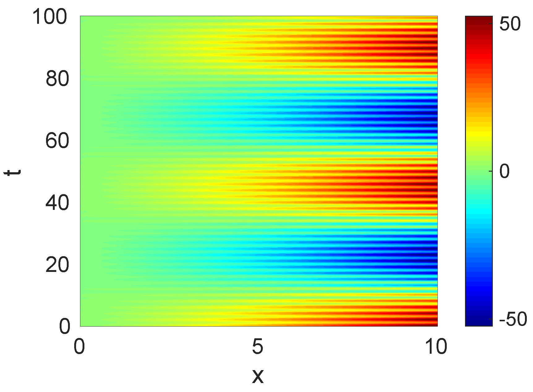
where and . Note that and are disparate from each other, which makes the associated dynamics multiscale and fairly demanding in the present context. This pattern is a slight modification of a toy model introduced in [30] and can be cast into the form (1) involving 4 frequencies, namely and . The model is temporally quasi-periodic because and are incommensurable (namely, the ratio is not a rational number). Figure 1 shows the spatio-temporal color map of the toy model.
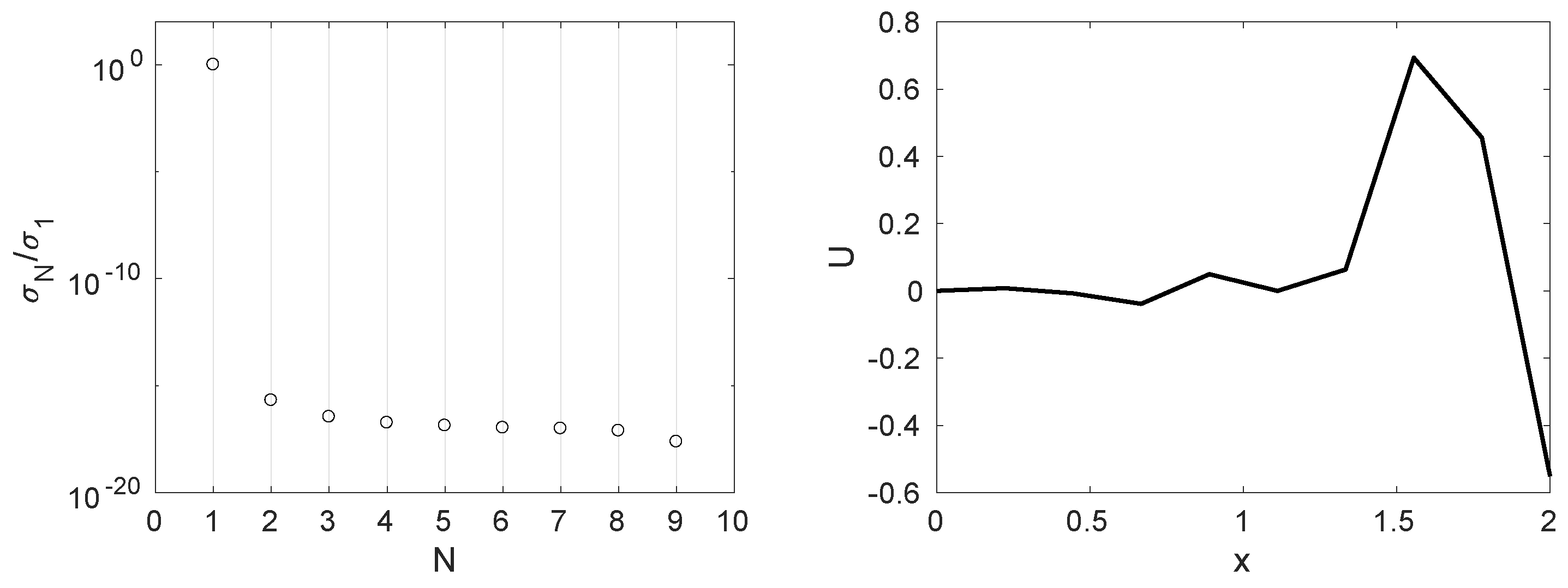
The HODMD method has been applied in 150 snapshots, collected in the time interval , which barely covers one period of the smallest frequency (see Figure 1). The snapshots to apply HODMD are considered in the spatial interval using 10 equispaced points. For simplicity, the parameters set in the analysis are chosen to obtain the zero machine error (the toy model is noise-free), namely and for . Figure 2
left shows the singular values calculated in the dimension-reduction step of the method (see Section 2) for the toy model. As seen, the model can be approximated by a single SVD mode related to the first singular value, whose intensity is much larger than the remaining modes. Figure 2 right shows the dominant SVD mode along the spatial component. As seen, considering the model for values of , the solution can be adjusted by a linear correlation (as first approximation) and a quadratic correlation (as second approximation). This result agrees with the evolution in space of (11), where the spatial component is seen to be approximately linear in x for small values of x, quadratic in x for moderately larger values of x (the quadratic term is multiplied by ) and cubic for still larger values of x (the cubic term is multiplied by ).
According to our comments above, the HODMD method only retains one SVD mode. The method calculates 4 exact frequencies, and the RMSE (as defined in Equation (10)) of the reconstruction of the original data is ∼10. Once DMD expansion (1) is constructed, it is possible to predict the solution in the time interval (temporal extrapolation) with RMSE ∼10. On the other hand, more in the spirit of the present paper, it is possible to predict the solution for points outside the interval , where the HODMD method has been applied (spatial extrapolation), namely for, e.g., and .
Figure 3 shows the prediction of the signal at the aforementioned points using linear and quadratic approximations. As seen, for small values of x (), the linear prediction gives a good approximation, with a RMS error ∼. This prediction improves using the quadratic approximation, whose RMS error is ∼. However, this approximation worsens at where the linear approximation is not good enough, since it gives a RMS error ∼. However, the RMS error at his point for this prediction using the quadratic approximation is . It is remarkable the influence of the cubic term appearing in (11) in all these approximations, since the RMS error is never negligible even for the approximation at using the quadratic approximation. Using a cubic approximation will reduce such error to zero machine, but the purpose of this section is explaining the performance of the model that will be used for the prediction of LiDAR measurements (including spatial extrapolation) rather than optimizing the performance of the method in the toy model.
4. HODMD-Based Reduced Order Model for Wind Prediction in LiDAR Measurements
The DMD expansion (1) can be considered as a reduced order model (ROM) to predict the temporal evolution of the temporal patterns in a given spatio-temporal dynamics data set. However, in real LiDAR measurements, the prediction of the data in time is limited by some other constrains such as changes in wind velocity, the weather or the atmospheric conditions. Thus, an alternative methodology (described below) is needed to predict/extrapolate the spatial patterns. Considering (1), each one of the DMD modes can be extrapolated in one of the spatial directions (i.e., the streamwise component x or, in the case of the LiDAR measurements, where the spatial component corresponds to a plane of measurements, it is possible to extrapolate to a new plane of measurements, resulting in a new DMD expansion for the new component, which is similar to the previously calculated (1)). However, when the data are too complex, the number of DMD modes composing the expansion is very large (i.e., in (1)), and the extrapolation could be very expensive in terms of computational cost. A good alternative is to extrapolate the SVD modes obtained in the dimension reduction step of the HODMD algorithm described in Section 2. In general, the number of SVD modes retained is smaller than the number of DMD modes. Since the DMD modes are composed by a linear combination of the SVD modes, extrapolating the SVD modes is similar to extrapolate the DMD modes. Thus, the methodology employed for the spatial prediction is as follows:
- Step 1 of HODMD: dimension reduction. SVD is applied to the snapshot matrix (2). Two sub-steps are now needed:
- -
- Correlations in SVD modes. Each one of the SVD modes is analyzed observing their trend in space, looking for an appropriate type of correlation (e.g., linear or quadratic) to extrapolate.
- -
- Extrapolation in space. Based on the correlation proposed in the previous step, the SVD modes are extrapolated in space.
- Step 2 of HODMD. The DMD expansion (1) is created using the new SVD modes.
5. Results of the HODMD Method Applied to LiDAR Measurements
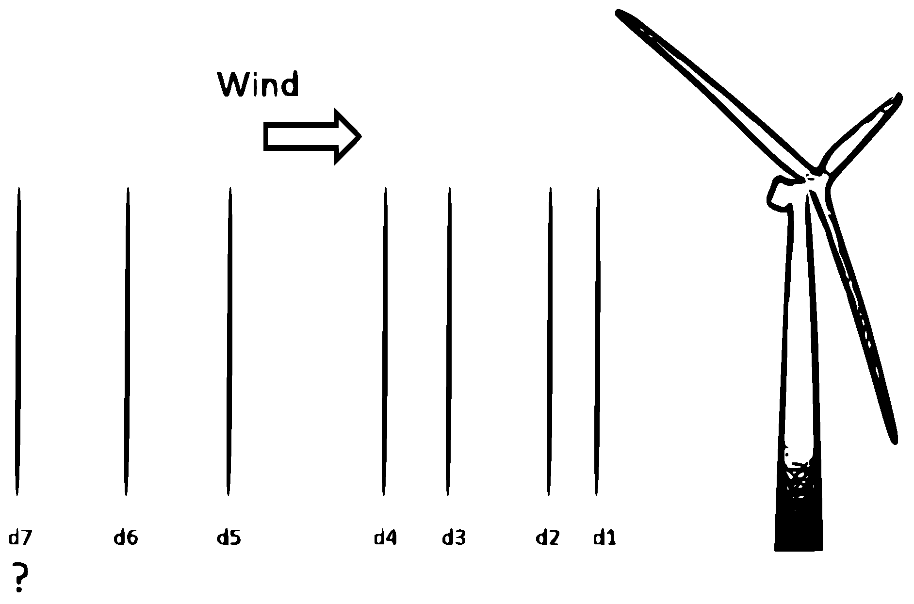
A LiDAR measurements campaign has been performed during 24 h near a horizontal axis wind turbine by the company ZephIR LiDAR [25]. Both the design and the location of the wind turbine are selected for maximizing wind power extraction, but cannot be described in this article for confidentiality reasons. Several sets of measurements have been carried out at six different distances upstream the wind turbine in the streamwise interval 33 m 201 m (for similar values of the transversal coordinate y). Predictions at distances larger than 200m are problematic, thus an HODMD-based ROM has been generated with the aim at predicting the wind velocity at 228 m. Figure 4 shows the distribution of the LiDAR measurements upstream the wind turbine. Two different sets of measurements have been carried out, at both sides of the wind turbine (left and right sides).
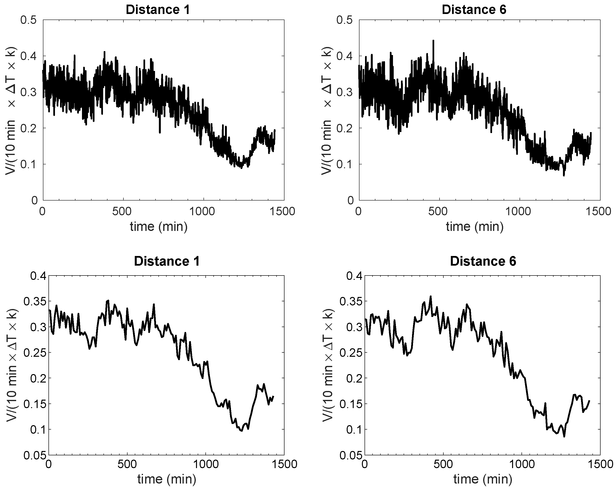
In order to overcome the difficulties usually triggered by the experimental measurements, between three and five sets of measurements are carried out in each distance, during time sub-intervals of ∼5 s. In order to reduce data uncertainty, these three to five values are promediated in time, for each distance. The original data are then organized as a group of measurements taken every s for all the distances. Hence, the database of LiDAR measurements contains a total number of 1500 groups of measurements (calculated as 24 h× 3600 s/h/57.5 s ) for each one of the 6 distances. Figure 5 top shows the original measurements in distances 1 and 6 (two representative points), for the set of data collected in the right side of the wind turbine. As seen, the data are quite noisy and the variations due to the velocity fluctuations are prominent. In order to attenuate the influence of the velocity fluctuations, a common practice to analyze LiDAR data in the wind energy industry is to promediate the data in timespans of 10 min [25]. The database is consequently reduced to a set of 144 promediated data groups (calculated as 1500/(10 min× 60 s/min/57.5 s) ≃144) for each distance. Figure 5 bottom shows the 10 min-promediated data for the same cases considered into the top plots. As seen, the trend of the data is maintained, but some of the larger fluctuations are filtered out.
HODMD has been applied to the promediated set of data. After some calibration, based on minimizing the RMS error for the reconstruction of the original data [23,29], the parameters used in the analysis are and retaining different number of singular values in the dimension-reduction step of the HODMD method (see Section 2). Figure 6 shows the singular values obtained in the first step of the HODMD algorithm for the set of data collected in the left and right sides of the wind turbine. As can be seen, the singular values for the left and right sides are very similar to each other. As expected, in each set of data, the method calculates 6 singular values, since the number of planes of measurements are 6. The magnitude (energy) of the 6th singular value is much smaller than the remaining ones. Namely, it is possible to obtain a good reconstruction of the original data retaining at most 5 SVD modes. The order of magnitude of modes 2 to 5 is similar, namely ∼, which makes difficult to distinguish any change in the tendency of the singular values, which could be related, for example, with the level of noise [31,32,33].
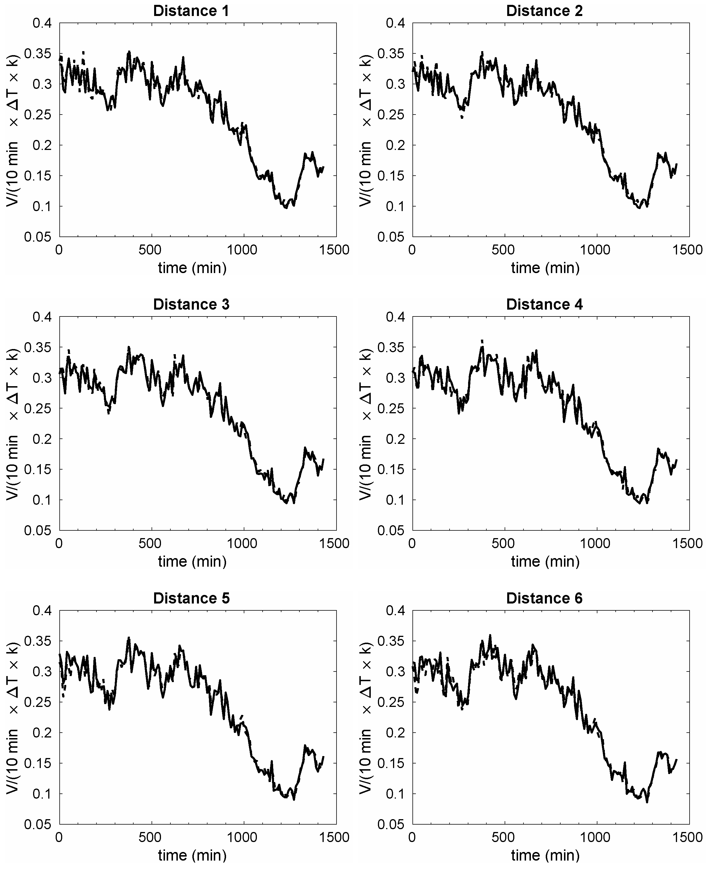
Several HODMD analyses have been performed retaining , 3, 4, and 5 singular values, retaining 73, 97, 95, and 95 DMD modes, respectively, which gives reconstruction errors of the original data ∼, ∼, ∼, and ∼, respectively, for the left set of data. Similarly, retaining the same numbers of singular values for the right set of data and retaining 69, 95, 93, and 99 DMD modes, respectively, the reconstruction errors are ∼, ∼, ∼, and ∼, respectively. Thus, could be considered as an optimal number of singular values to be retained, but calculations using singular values are also good, since the error is almost the same as for , but the number of DMD modes is smaller (simpler approximation of expansion (1)). Figure 7 shows the frequencies vs. their corresponding amplitudes and growth rates, obtained in these analyses, considering and , for the data collected in the left (top) and right (bottom) sides of the wind turbine. As seen, not only the frequencies calculated in the left and right data sets are different, but also some differences are found in the calculations of the growth rates. It is remarkable that the LiDAR signal is composed by a large number of modes, some of them decreasing (negative growth rates) and some of them increasing (positive growth rates) in time. In both data sets, most of the modes are calculated with damping rates contained in the range . However, in the left data set, these modes are more dispersed in the interval, while in the right data set, a larger number of modes is gathered in , meaning that the signal is slightly more complex in the left data set (larger diversity in the dynamics). Figure 8 and Figure 9 show the reconstruction of the signal using 4 SVD modes in the six planes of measurements, for the left and right data sets, respectively. As seen, the results obtained match quite well with the original solution. The larger (though still reasonable) discrepancies are found at times larger than 1000 min. The reason is that there is a change of tendency in the data at this region. At times smaller than 1000 min, the dynamics are decaying, while after this time, a new dynamic behavior is developed, which is still growing. If the data set analyzed were larger, HODMD would have better approximated this emerging dynamic.
Prediction in LiDAR Measurements
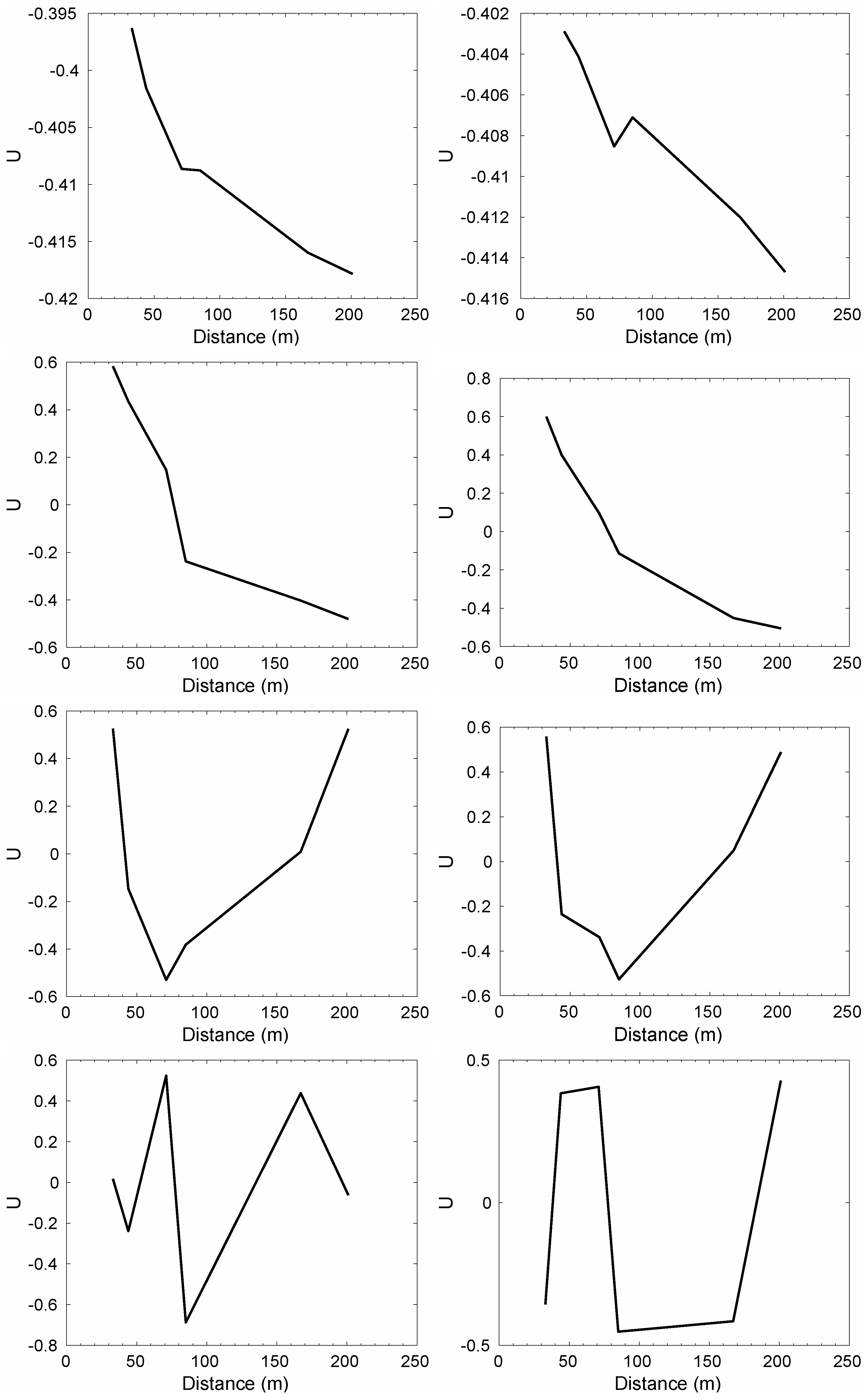
Once the method is proved to reconstruct the original signal with an error ∼5%, the same DMD expansion (1) is used to predict the velocity in a new plane at a larger distance, namely at m, which will be made as explained in Section 4. As explained in this section, it is necessary to first analyze the SVD modes, in order to adjust a model that optimizes extrapolation. Figure 10 shows the four SVD modes that are retained according to our comments above, as calculated for the right and left data sets.
As can be seen, the first three modes behave fairly linearly for distances m, suggesting that a quadratic or even linear extrapolation could be sufficient.
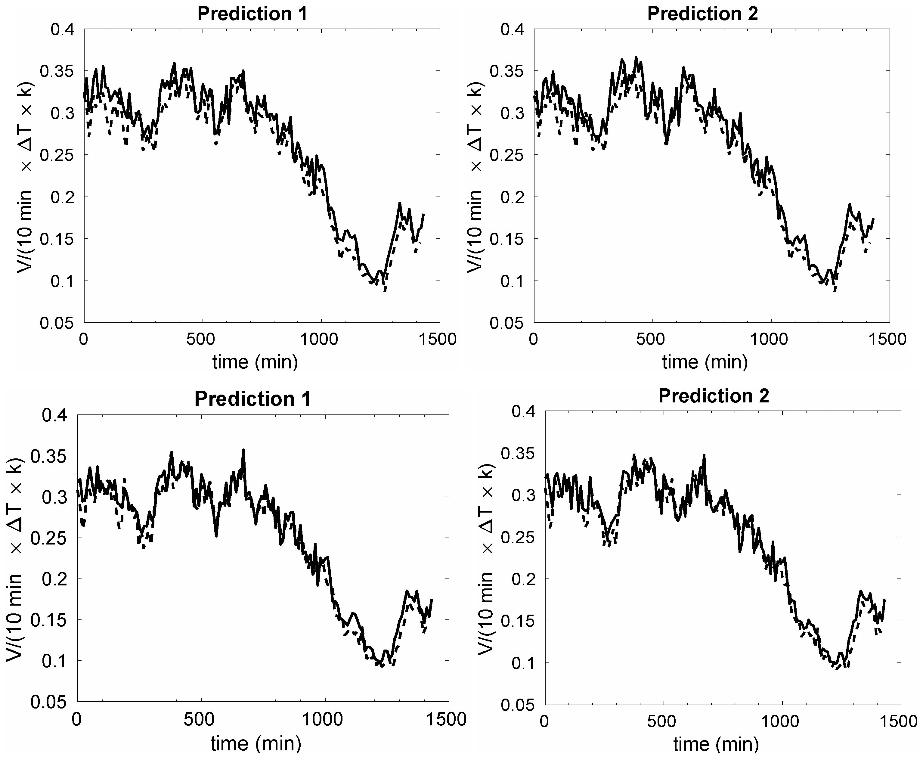
Two different models, linear and quadratic, have been used to extrapolate the spatial DMD modes to m. Figure 11 compares the resulting predictions with the actual LiDAR measurements at this new distance in the left and right data sets. As seen, the results using linear and quadratic extrapolation are similar among each other, which is consistent with our comment above on the behavior of the DMD modes. This is also consistent with what we obtained for the toy model presented in Section 3. In other words, in near field extrapolations (228m is not far away from the distance m), linear and quadratic models provide similar solutions. In contrast, it would be necessary to increase the order of the model in the far field (quadratic, cubic,⋯) to extrapolate to distances larger than 228m. Instead, for the present case, the linear and quadratic extrapolations give reasonably good results (see Figure 11), since the RMS error for the wind prediction is ∼7% in all the cases presented. It is remarkable that this error is only 2% larger than the one previously calculated using this model for the reconstruction of the original data (based on the model proposed, the minimum error for data prediction could be 5%). This fact shows the good performance of this new HODMD-based model used for data forecasting. The prediction for the right data set is slightly better than that for the left data set. As shown above (Figure 7), the diversity of the modes and growth rates obtained in the calculations is larger in the left set, proving the major complexity of the data, which explains the difficulties found in this analysis. It is also remarkable that, the new signal is better predicted at times smaller than 1000 min. This result agrees with the reconstruction of the signal presented before.
6. Conclusions
A new method has been proposed to predict wind velocities upstream a horizontal axis wind turbine from a set of data collected from LiDAR experiments. The method uses HODMD as a ROM and extrapolates in space the SVD modes, which are used to construct the spatial DMD modes.
Firstly, the method has been tested in a toy model, quasi-periodic in time, and whose spatial behavior depends on a cubic equation. Secondly, the HODMD-based ROM has been used to approximate a set of data obtained from actual LiDAR experiments as an expansion of DMD modes. The experimental data have been taken at 6 different distances upstream the wind turbine, in the interval 33 m 201 m. The original data have been reconstructed by means of a DMD expansion of the type (1) obtained via an iterative HODMD method. The RMS error of the reconstruction was ∼5% in all the planes, proving the good performance of the method.
Finally, once that expansion (1) is accurately calculated, the HODMD-based ROM is used to predict the wind velocity outside the interval where the actual LiDAR measurements were performed, at m. The prediction has been compared to original LiDAR measurements and the error of the calculations is ∼7%, only 2% larger than the minimum error for the model proposed. The method has been tested in two different sets of data, collected at both sides of the wind turbine. The results obtained are similar in both cases showing the robustness and the suitable performance of this HODMD-based ROM for wind predictions upstream horizontal axis wind turbines analyzing data coming from LiDAR measurements. In addition, the technique introduced is general and robust, as HODMD, making possible to extend its application to vertical axis wind turbines. It is also remarkable that the computational cost required to obtain and apply the HODMD-based ROM is almost negligible. This opens the possibility for using this method for real-time calculations, which is a very interesting application for the wind industry.
Acknowledgments
This work was partially supported by the Spanish Ministry of Economy and Competitiveness, under grant TRA2016-70750-R. The authors are also in debt with CarloAlberto Ratti, from the company ZephIR LiDAR [25], for providing us with the actual LiDAR data analyzed in this article.
Author Contributions
Soledad Le Clainche, Luis S. Lorente and José M. Vegacontributed in the development of the idea and in the development and coding of the method. Soledad Le Clainche analyzed the data. Luis S. Lorente studied the physical problem. José M. Vega contributed with global ideas. Soledad Le Clainche, Luis S. Lorente and José M. Vega wrote the paper.
Conflicts of Interest
The authors declare no conflict of interest.
References
- Harris, M.; Hand, M.; Wright, A. A Lidar for Turbine Control; Technical Report NREL/TP-500-39154; National Renewable Energy Laboratory (NREL): Golden, CO, USA, 2006. [Google Scholar]
- Karlsson, C.J.; Olsson, F.A.A.; Letalick, D.; Harris, M. All-fiber multifunction continuous-wave coherent laser radar at 1.55 μm for range, speed, vibration, and wind measurements. Appl. Opt. 2000, 39, 3716–3726. [Google Scholar] [CrossRef] [PubMed]
- Banakh, V.A.; Smalikho, I.N.; Köpp, F.; Werner, C. Representativeness of wind measurements with a cw Doppler lidar in the atmospheric boundary layer. Appl. Opt. 1995, 34, 2055–2067. [Google Scholar] [CrossRef] [PubMed]
- Mikkelsen, T.; Hansen, K.; Angelou, N.; Sjöholm, M.; Harris, M.; Hadley, P.; Scullion, R.; Ellis, G.; Vives, G.; Risø, D.T.U.; et al. Lidar wind speed measurements from a rotating spinner. In Proceedings of the European Wind Energy Conference, Warsaw, Poland, 20–23 April 2010. [Google Scholar]
- Li, J.; Yu, X.B. LiDAR technology for wind energy potential assessment: Demonstration and validation at a site around Lake Erie. Energy Convers. Manag. 2017, 144, 252–261. [Google Scholar] [CrossRef]
- Smith, D.A.; Harris, M.; Coffey, A.S.; Mikkelsen, T.; Jørgensen, H.E.; Mann, J.; Danielian, R. Wind lidar evaluation at the Danish wind test site in Høvsøre. Wind Energy 2006, 9, 87–93. [Google Scholar] [CrossRef]
- Kim, D.; Kim, T.; Oh, G.; Huh, J.; Ko, K. A comparison of ground-based LiDAR and met mast wind measurements for wind resource assessment over various terrain conditions. J. Wind Eng. 2016, 158, 109–121. [Google Scholar] [CrossRef]
- Peña, A.; Hasager, C.B.; Gryning, S.E.; Courtney, M.; Antoniou, I.; Mikkelsen, T. Offshore wind profiling using light detection and ranging measurements. Wind Energy 2009, 12, 105–124. [Google Scholar] [CrossRef]
- Harris, M.; Bryce, D.J.; Coffey, A.S.; Smith, D.A.; Birkemeyer, J.; Knopf, U. Advance measurement of gusts by laser anemometry. J. Wind Eng. 2007, 95, 1637–1647. [Google Scholar] [CrossRef]
- Power Performance of Measurements of Electricity Producing Wind Turbines; IEC 61400-12-1; International Electrotechnical Commission: Geneva, Switzerland, 2005.
- Wagner, R.; Courtney, M.; Gottschall, J.; Lindelöw-Marsden, P. Accounting for the speed shear in wind turbine power performance measurement. Wind Energy 2011, 14, 993–1004. [Google Scholar] [CrossRef]
- Wagner, R.; Pedersen, T.F.; Courtney, M.; Antoniou, I.; Davoust, S.; Rivera, R.L. Power curve measurement with a nacelle mounted lidar. Wind Energy 2014, 17, 1441–1453. [Google Scholar] [CrossRef]
- Wang, N.; Wright, A.D.; Balas, M.J. Disturbance Accommodating Control Design for Wind Turbines Using Solvability Conditions. ASME J. Dyn. Sys. Meas. Control 2017, 139. [Google Scholar] [CrossRef]
- Wright, A.D.; Balas, M.J. Design of Controls to Attenuate Loads in the Controls Advanced Research Turbine. ASME J. Sol. Energy Eng. 2004, 126, 1083–1091. [Google Scholar] [CrossRef]
- Pace, A.; Johnson, K.; Wright, A. Preventing wind turbine overspeed in highly turbulent wind events using disturbance accommodating control and light detection and ranging. Wind Energy 2015, 18, 351–368. [Google Scholar] [CrossRef]
- Wang, N.; Johnson, K.E.; Wright, A.D.; Carcangiu, C.E. Lidar-assisted wind turbine feedforward torque controller design below rated. In Proceedings of the American Control Conference, Portland, OR, USA, 4–6 June 2014; pp. 3728–3733. [Google Scholar]
- Schlipf, D.; Fleming, P.; Haizmann, F.; Scholbrock, A.; Hofsäß, M.; Wright, A.; Cheng, P.W. Field Testing of Feedforward Collective Pitch Control on the CART2 Using a Nacelle-Based Lidar Scanner. J. Phys. Conf. Ser. 2014, 555. [Google Scholar] [CrossRef]
- Scholbrock, A.; Fleming, P.; Fingersh, L.; Wright, A.; Schlipf, D.; Haizmann, F.; Belen, F. Field Testing LIDAR-Based Feed-Forward Controls on the NREL Controls Advanced Research Turbine. In Proceedings of the 51st AIAA Aerospace Sciences Meeting including the New Horizons Forum and Aerospace Exposition, Aerospace Sciences Meetings, Grapevine, TX, USA, 7–10 January 2013. [Google Scholar]
- Le Clainche, S.; Vega, J.M. Higher Order Dynamic Mode Decomposition. SIAM J. Appl. Dyn. Syst. 2017, 16, 882–925. [Google Scholar] [CrossRef]
- Schmid, P.J. Dynamic mode decomposition of numerical and experimental data. J. Fluid Mech. 2010, 656, 5–28. [Google Scholar] [CrossRef] [Green Version]
- Takens, F. Detecting Strange Attractors in Turbulence. In Lecture Notes in Mathematics; Rand, D.A., Young, L.-S., Eds.; Springer: Berlin, Germany, 1981; pp. 366–381. [Google Scholar]
- Le Clainche, S.; Vega, J.M. Higher order dynamic mode decomposition to identify and extrapolate flow patterns. Phys. Fluids 2017, 29. [Google Scholar] [CrossRef]
- Le Clainche, S.; Vega, J.M.; Soria, J. Higher Order Dynamic Mode Decomposition for noisy experimental data: flow structures on a Zero-Net-Mass-Flux jet. Exp. Therm. Fluid Sci. 2017, 88, 336–353. [Google Scholar] [CrossRef]
- Le Clainche, S.; Moreno-Ramos, R.; Taylor, P.; Vega, J.M. A new robust method to study flight flutter testing. J. Aircr. submitted.
- ZephIR Lidar. Fairoaks Farm, Hollybush, Ledbury, HR8 1EU, UK. Available online: https://www.zephirlidar.com (accessed on 3 March 2018).
- Sirovich, L. Turbulence and the dynamic of coherent structures, parts I–III. Q. Appl. Math. 1987, 45, 561–590. [Google Scholar] [CrossRef]
- Golub, G.H.; van Loan, G.T. Matrix Computations; John Hopkins University Press: Baltimore, MD, USA, 1996. [Google Scholar]
- Stewart, G.W. Error and perturbation bounds for subspaces associated with certain eigenvalue problems. SIAM Rev. 1973, 15, 727–764. [Google Scholar] [CrossRef]
- Le Clainche, S.; Sastre, F.; Vega, J.M.; Velázquez, A. Higher order dynamic mode decomposition applied to postproces a limited amount of PIV data. In Proceedings of the 47th AIAA Fluid Dynamics Conference, AIAA Aviation Forum, Denver, CO, USA, 5–9 June 2017. AIAA paper 2017-3304. [Google Scholar]
- Giannakis, D.; Slawinska, J.; Zhao, Z. Spatio-temporal feature extraction with data-driven Koopman operators. J. Mach. Learn. Res. 2015, 44, 103–115. [Google Scholar]
- Le Clainche, S.; Varas, F.; Vega, J.M. Accelerating oil reservoir simulations using POD on the fly. Int. J. Numer. Methods Eng. 2017, 79, 79–100. [Google Scholar] [CrossRef]
- Le Clainche, S.; Vega, J.M. Spatio Temporal Koopman Decomposition. J. Nonlinear Sci. 2018, in press. [Google Scholar]
- Rapun, M.-L.; Terragni, F.; Vega, J.M. LUPOD: Collocation in POD via LU decomposition. J. Comput. Phys. 2017, 335, 1–20. [Google Scholar] [CrossRef]
Figure 1.
Toy model (11).
Figure 1.
Toy model (11).

Figure 2.
Singular values (left) and first SVD mode (right) calculated in the toy model (11).
Figure 2.
Singular values (left) and first SVD mode (right) calculated in the toy model (11).

Figure 3.
Predictions in the toy model (11). (Left) linear approximation. (Right) quadratic approximation. Continuous and dashed lines represent the original solution and the prediction, respectively.
Figure 3.
Predictions in the toy model (11). (Left) linear approximation. (Right) quadratic approximation. Continuous and dashed lines represent the original solution and the prediction, respectively.
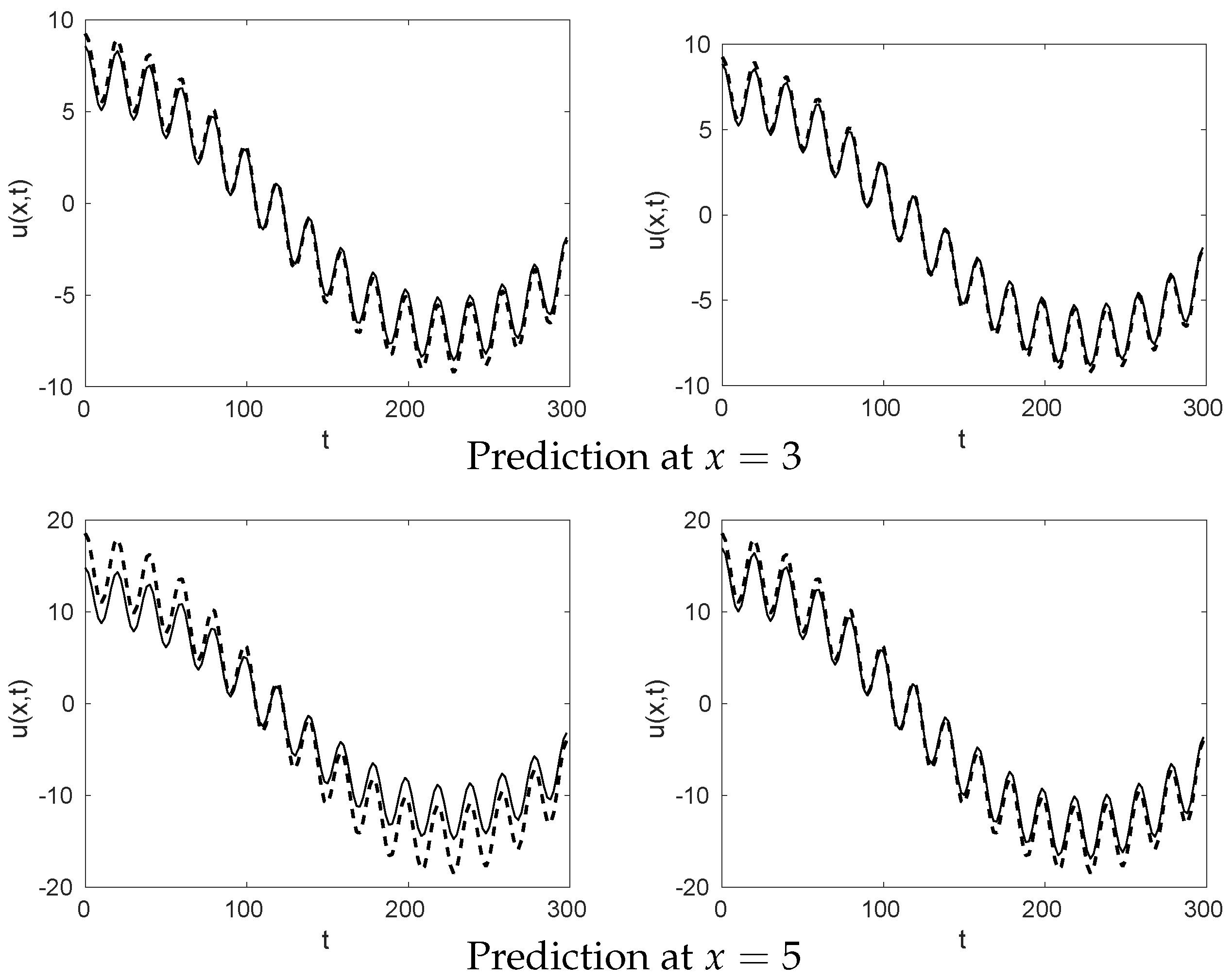
Figure 4.
Plane of measurements upstream the wind turbine in the LiDAR experimental campaign. Data are available in the six planes that are closer to the wind turbine, while the data on the seventh plane are to be predicted.
Figure 4.
Plane of measurements upstream the wind turbine in the LiDAR experimental campaign. Data are available in the six planes that are closer to the wind turbine, while the data on the seventh plane are to be predicted.

Figure 5.
LiDAR measurements obtained upstream the wind turbine (right side) at distances 1 (left) and 6 (right). Top: raw measurements. Bottom: measurements promediated every 10 min. (Herein and in what follows, all the velocity fields are escaled with a factor k).
Figure 5.
LiDAR measurements obtained upstream the wind turbine (right side) at distances 1 (left) and 6 (right). Top: raw measurements. Bottom: measurements promediated every 10 min. (Herein and in what follows, all the velocity fields are escaled with a factor k).

Figure 6.
Singular values calculated in the data sets obtained in the left and right sides of the wind turbines, represented by crosses and circles, respectively.
Figure 6.
Singular values calculated in the data sets obtained in the left and right sides of the wind turbines, represented by crosses and circles, respectively.
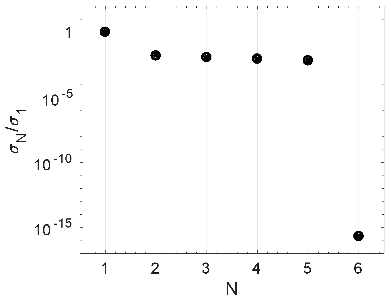
Figure 7.
Frequencies vs. amplitudes (left) and growth rates (right) in the HODMD analysis for the data collected in the left (top) and right (bottom) sides. Crosses and circles represent the analysis carried out retaining and singular values, respectively.
Figure 7.
Frequencies vs. amplitudes (left) and growth rates (right) in the HODMD analysis for the data collected in the left (top) and right (bottom) sides. Crosses and circles represent the analysis carried out retaining and singular values, respectively.
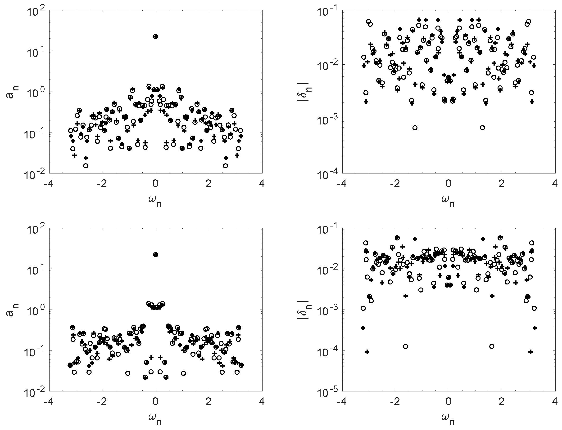
Figure 8.
Original (solid lines) and HODMD-reconstruction (dashed lines) of the LiDAR measurements using the DMD expansion (1) for the right set of measurements using 4 singular values.
Figure 8.
Original (solid lines) and HODMD-reconstruction (dashed lines) of the LiDAR measurements using the DMD expansion (1) for the right set of measurements using 4 singular values.

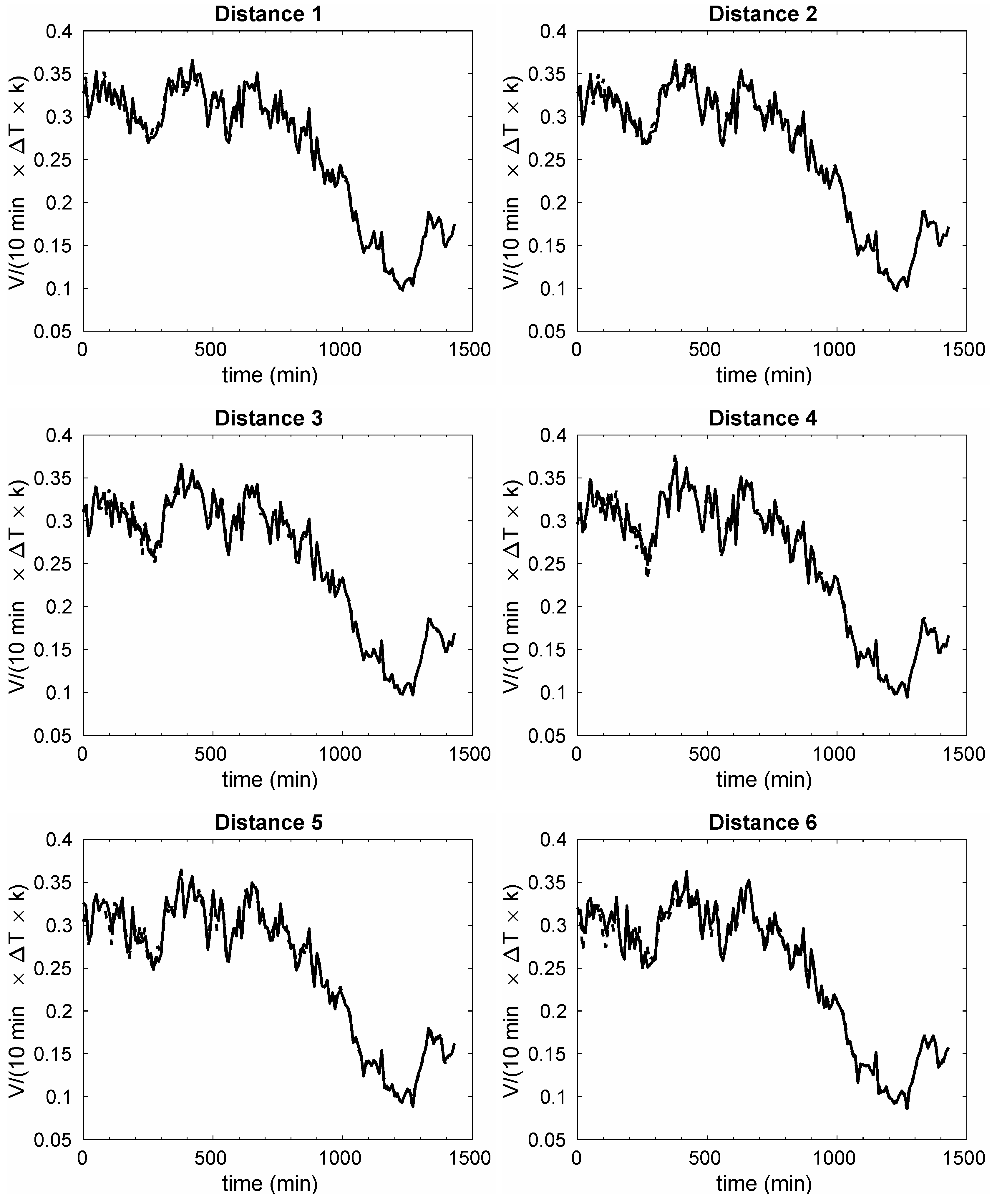
Figure 9.
Counterpart of Figure 8 for the left set of measurements
Figure 9.
Counterpart of Figure 8 for the left set of measurements

Figure 10.
SVD modes calculated in the data sets obtained in the left (left) and right (right) sides of the wind turbines. From top to bottom: modes 1 to 4.
Figure 10.
SVD modes calculated in the data sets obtained in the left (left) and right (right) sides of the wind turbines. From top to bottom: modes 1 to 4.

Figure 11.
Original (solid lines) and HODMD-predictions (dashed lines) of the wind velocity upstream the wind turbine at m using a linear (left) and quadratic (right) approximation model. Top: data set from the left side of the wind turbine. Bottom: data set from the right side of the wind turbine.
Figure 11.
Original (solid lines) and HODMD-predictions (dashed lines) of the wind velocity upstream the wind turbine at m using a linear (left) and quadratic (right) approximation model. Top: data set from the left side of the wind turbine. Bottom: data set from the right side of the wind turbine.
© 2018 by the authors. Licensee MDPI, Basel, Switzerland. This article is an open access article distributed under the terms and conditions of the Creative Commons Attribution (CC BY) license (http://creativecommons.org/licenses/by/4.0/).
Share and Cite
MDPI and ACS Style
Le Clainche, S.; Lorente, L.S.; Vega, J.M. Wind Predictions Upstream Wind Turbines from a LiDAR Database. Energies 2018, 11, 543. https://doi.org/10.3390/en11030543
AMA Style
Le Clainche S, Lorente LS, Vega JM. Wind Predictions Upstream Wind Turbines from a LiDAR Database. Energies. 2018; 11(3):543. https://doi.org/10.3390/en11030543
Chicago/Turabian StyleLe Clainche, Soledad, Luis S. Lorente, and José M. Vega. 2018. "Wind Predictions Upstream Wind Turbines from a LiDAR Database" Energies 11, no. 3: 543. https://doi.org/10.3390/en11030543
Note that from the first issue of 2016, this journal uses article numbers instead of page numbers. See further details here.