AC and DC Impedance Extraction for 3-Phase and 9-Phase Diode Rectifiers Utilizing Improved Average Mathematical Models

Abstract

Switching models possess discontinuous and nonlinear behavior, rendering difficulties in simulations in terms of time consumption and computational complexity, leading to mathematical instability and an increase in its vulnerability to errors. This issue can be countered by averaging detailed models over the entire switching period. An attempt is made for deriving improved dynamic average models of three phase (six-pulse) and nine phase (18-pulse) diode rectifiers by approximating load current through first order Taylor series. Small signal AC/DC impedances transfer functions of the average models are obtained using a small signal current injection technique in Simulink, while transfer functions are obtained through identification of the frequency response into the second order system. For the switch models in Simulink and the experimental setup, a small signal line to line shunt current injection technique is used and the obtained frequency response is then identified into second order systems. Sufficient matching among these results proves the validity of the modelling procedure. Exact impedances of the integral parts, in interconnected AC/DC/AC systems, are required for determining the stability through input-output impedances.

1. Introduction

The demand for power electronic converters has increased with the dependence on electronic appliances, digital products and computer systems in both industrial and household applications [1]. Power converters are required almost in every field that deals with electronics such as aircrafts, sea ships, communication systems, renewable energy generations, such as wind generation systems, photovoltaic systems and fuel cells etc. [2,3]. Since past few decades, engineers and scientists have focused on developing new control techniques as well as efficient models for various power converters so that to meet the IEEE prescribed standards, reliability and performance. Multi-pulse AC/DC converters are found to be one of the best solutions for providing loads with output voltages and currents having less ripples, reliable as well as rarely polluting the ac supply sources. These converters help in keeping lower total harmonic distortion (THD) at the ac side and hence less power consumption for the rated devices. The most common type of multi-pulse converter is the conventional six-pulse (three-phase) line-commutated rectifier, typically used as the input stage in low-to-medium-power variable frequency drives and motor loads common in industrial and commercial applications [4,5,6]. However, an increased number of pulses is employed for improved performance, comprising of auto-transformers (converts three phase supply into n-phase system) feeding n/3 number of 3-phase rectifiers connected in parallel/series [7,8,9]. The switching nature of detailed model makes it less favorable to be simulated for testing with experimental prototypes. These models are time consuming, discontinuous in nature, nonlinear in behavior and causes mathematical instabilities due to complex computations [10,11,12,13].

Average models have been found to be the best tools for overcoming these issues by reducing time span for testing and simulation of the models with sufficiently matching results to those of detailed models [14,15]. The power engineering community has remained very prudent while deriving average models of these rectifiers. The resulting models have been investigated quite extensively proving sufficient accuracy for various applications. There are two ways of implementing these models namely, explicit mathematical model and transfer function method [16,17]. Prior method requires knowledge and proper calculations of all the constraints involved in modelling while later method requires extraction of the relationship between the input and output terms using simulation of the detailed/hardware prototype extensively over different load conditions. Once data is extracted, coefficients of parameters are approximated into polynomials which are used in model. In [18,19], partial dynamic improvement in model was achieved by considering linearly varying load current. The dynamic average value models (AVMs) have been utilized effectively to remove the high-frequency switching from detailed models while preserving the lower frequency dynamics of the systems. Validity of any model developed is based upon the matching results during static and dynamic conditions with those of hardware prototypes/detailed models. These models are faster and applicable for extraction of impedance transfer functions which are utilized in stability analysis.

The active nature of power electronics converters results in complex dynamic behavior during interconnection. It makes the system level analysis of interconnected converters much more complicated [20,21]. Power electronic devices are normally designed to supply non-negative resistive loads but due to negative impedance impact offered by constant power loads in tightly controlled power systems they are more prone to instabilities [22,23,24,25]. The classical and most efficient way to determine the stability of a complex interconnected EPS is to examine the Nyquist contour of the return ratio (product of output impedance of system 1 and that of admittance of system 2) of the two interconnected systems [21,26,27] as shown in Figure 1. This has led to the use of impedance techniques for stability analysis in power supply designs along with number of stability criterions involving magnitude and phase [28]. It is imperative to obtain the linearized input/output impedances transfer functions of each integral component within complex systems. Converter impedance is obtained by considering the control dynamics [29]. Impedance-based stability for both the direct current (DC) [30] and AC systems are assessed in [31,32,33,34,35,36,37,38,39,40,41]. One way to obtain impedance of a system is to inject signal of appropriate magnitude and frequency to obtain the frequency response through Fourier transform. This would need one signal injection for single frequency response in case of DC while requiring two linearly independent injections for single point frequency response measurement in ac systems [42]. For ac system, ABC model (three-axes coordinate system) is converted into DQ synchronous reference frame (two-axes coordinate system) and then linearized AVM of the specified system is utilized to obtain the small signal transfer functions for the input/output impedances, required for stability measurements. These transfer functions can be validated by comparing with those of prototypes or detailed models by applying impedance extraction techniques discussed in [43].

This paper proposes an improvement in the static models derived in [44,45], where load current is treated as a constant dc value. Linear variation in dc load current is taken into account which adds the extra term “K” to model equations. Adding this linear term to the models’ derivation procedure makes it closer to the detailed models during transient states. Static models perform well during steady states but fail to capture the dynamics of the system during transient state. Using this concept, improved dynamic average value models have been developed for 3-phase and 9-phase diode rectifiers using first order Taylor series expansion of the load current ($I_{dc}$) so that to capture the dynamics of the system as well. These AVMs are linearized to obtain small signal transfer functions of the input/output impedances of the rectifiers through identification process and tested under steady and dynamic states. The dc side of the rectifier (output) has only one impedance parameter “$Z_{out}$” while ac side has four parameters which are$Z_{dd}$,$Z_{dq}$,$Z_{qd}$,$Z_{qq}$. Extracting exact impedances transfer functions is the main goal of all research focused in this area since these are required for stability analysis of interconnected systems. Comparison of these transfer functions with those obtained from the detailed models as well as hardware prototypes reveals the validity and efficiency of the proposed average value models.

2. Mathematical Average Value Models

In static models, load current is assumed to be constant dc but in actual, it varies according to load variation. It is therefore required to develop such a model which brings the load variation into consideration so that the model is much in accordance to that of real circuit under steady state as well as dynamic state.

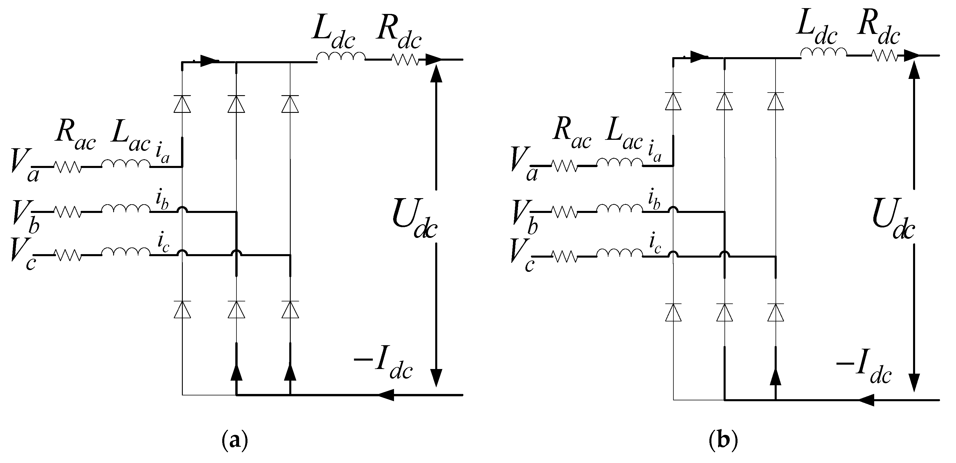
2.1. Dynamic Average Value Model of 3-Phase Diode Rectifiers

For a three-phase rectifier with parameters given in

Table 1. Circuit parameters.

No.	Parameter	Values
1	Frequency	400 Hz
2	Power	2048 Watts
3	Input Voltage (Vin)	115 Vrms
4	$L_{dc}$	8 mH
5	$L_{ac}$	500 µH
6	$R_{dc}$	10 mΩ
7	$R_{ac}$	20 mΩ
8	$\mathrm{Load}\mathrm{Resistance}$	32 Ω

, µ representing commutation angle, $I_{dc0}$ representing the average value of $I_{dc}$ and K representing the rate of load current variation during this period of time ($d{I}_{dc}/d\omega t$), assume that load current varies linearly and is represented by evaluating first order Taylor series as:

$$I_{dc}\left(\theta \right)=I_{dc0}+K\left(\theta -\frac{\mu }{2}\right)$$

(1)

Commutation and conduction periods of a three-phase rectifier are shown in Figure 2a,b, along with the current waveforms in Figure 3. Current waveforms are trapezoidal shaped since inductors used at dc side, filters out peak lobes hence feeding load with constant DC current. Although, commutation period is affected by the higher filtering inductor value which could cause spikes in load voltage but proper selection of dc filter values could be the ultimate solution. Considering $V_m$ as the peak value of supply voltages given by Equation (2),

$$\begin{array}{c}{V}_a=V_m\sin \left(\theta +\frac{\pi }{2}\right)\\ V_b=V_m\sin \left(\theta -\frac{\pi }{6}\right)\\ V_c=V_m\sin \left(\theta -\frac{5\pi }{6}\right)\end{array}\}$$

(2)

From the circuit in Figure 2 during commutation period, considering$R_{ac},L_{ac}$ to be the resistance and inductance on the ac side while $R_{dc},L_{dc}$ be the resistance and inductance on the dc side, $U_p$ and $U_n$ representing the positive and negative terminal potentials with respect to neutral point of the rectifier ac supply, system dynamic equations are:

$$\begin{array}{lll}{V}_a=R_{ac}{i}_a+L_{ac}\frac{d{i}_a}{dt}+U_p& \mathrm{and}& i_a=I_{dc}\\ V_b=R_{ac}{i}_b+L_{ac}\frac{d{i}_b}{dt}+U_n& \mathrm{and}& i_b+i_c=-I_{dc}\\ V_c=R_{ac}{i}_c+L_{ac}\frac{d{i}_c}{dt}+U_n& & \end{array}\}$$

(3)

$$U_p-U_n=R_{dc}{I}_{dc}+L_{dc}\frac{d{I}_{dc}}{dt}+U_{dc}$$

(4)

Now during conduction period, system dynamic equations are:

$$\begin{array}{l}{V}_a=R_{ac}{i}_a+L_{ac}\frac{d{i}_a}{dt}+U_p\mathrm{and}{i}_a=I_{dc}\\ V_c=R_{ac}{i}_c+L_{ac}\frac{d{i}_c}{dt}+U_n\mathrm{and}{i}_b=0,i_c=-I_{dc}\end{array}\}$$

(5)

$$U_p-U_n=R_{dc}{I}_{dc}+L_{dc}\frac{d{I}_{dc}}{dt}+U_{dc}$$

(6)

Solving the above equations for$U_p$, $U_n$ and rearranging,

$$\frac{d{I}_{dc}}{dt}=-\frac{\left(R_{dc}+\frac{3}{2}{R}_{ac}\right)}{\left(L_{dc}+\frac{3}{2}{L}_{ac}\right)}\left(I_{dc0}+K\left(\theta -\frac{\mu }{2}\right)\right)+\frac{3V_a}{2\left(L_{dc}+\frac{3}{2}{L}_{ac}\right)}-\frac{U_{dc}}{\left(L_{dc}+\frac{3}{2}{L}_{ac}\right)}$$

(7)

$$\frac{d{I}_{dc}}{dt}=-\frac{\left(R_{dc}+2R_{ac}\right)}{\left(L_{dc}+2L_{ac}\right)}\left(I_{dc0}+K\left(\theta -\frac{\mu }{2}\right)\right)+\frac{\sqrt{3}{V}_m\cos \left(\theta -\frac{\pi }{6}\right)}{\left(L_{dc}+2L_{ac}\right)}-\frac{U_{dc}}{\left(L_{dc}+2L_{ac}\right)}$$

(8)

Integrating (7) over 0 to $\mu$ and (8) over $\mu \mathrm{to}\raisebox{1ex}{$\pi $}\!\left/ \!\raisebox{-1ex}{$3$}\right.$

$$\frac{d{I}_{dc}}{dt}=-\frac{\left(R_1\right)}{\left(L_1\right)}\mu I_{dc0}+\frac{3V_m\sin \left(\mu \right)}{2\left(L_1\right)}-\frac{\mu U_{dc}}{\left(L_1\right)}$$

(9)

$$\begin{gathered} \frac{d{I}_{dc}}{dt}=-\left(\frac{\pi }{3}\right)\frac{R_2}{L_2}{I}_{dc0}+\frac{R_2}{L_2}\mu I_{dc0}-\frac{R_{2}K{\pi }^2}{18L_2}+\frac{R_{2}K{\mu }^2}{2L_2}+\left(\frac{\pi }{3}\right)\frac{R_{2}K\mu }{2L_2}-\frac{R_{2}K{\mu }^2}{2L_2}+\frac{3V_m}{2L_2}\left(\frac{\sqrt{3}}{2}\right) \\ -\frac{3V_m}{2L_2}\sin \left(\mu \right)-\frac{\sqrt{3}{V}_m}{2L_2}\left(\frac{1}{2}\right)+\frac{\sqrt{3}{V}_m}{2L_2}\cos \left(\mu \right)-\frac{U_{dc}}{3L_2}\pi +\frac{\mu U_{dc}}{L_2} \end{gathered}$$

(10)

where $R_1=R_{dc}+\frac{3}{2}{R}_{ac},L_1=L_{dc}+\frac{3}{2}{L}_{ac},R_2=R_{dc}+2R_{ac}$ and $L_2=L_{dc}+2L_{ac}$

Averaging (9) and (10) over $0\to \frac{\pi }{3}$

$$\begin{gathered} \frac{d{I}_{dc}}{dt}=-\frac{3}{\pi }\left(\left(\frac{R_1}{L_1}-\frac{R_2}{L_2}\right)\mu +\frac{R_2}{L_2}\right)I_{dc0}+\frac{3}{\pi }\left(\frac{3}{2L_1}sin\left(\mu \right)+\frac{\sqrt{3}}{2L_2}-\frac{\sqrt{3}}{L_2}sin\left(\mu -\frac{\pi }{6}\right)\right)V_m \\ -\left(\frac{3}{\pi }\left(\frac{1}{L_1}-\frac{1}{L_2}\right)\mu +\frac{1}{L_2}\right)U_{dc} \end{gathered}$$

(11)

AC Current Equation

During commutation period, it can be seen from Figure 2a that

$$\begin{array}{c}{i}_a\left(\theta \right)=I_{dc}\left(\theta \right)=I_{dc0}+K\left(\theta -\frac{\mu }{2}\right)\\ i_b\left(\theta \right)=-\frac{\sqrt{3}{V}_m}{2\omega L_{ac}}\left(\cos (\theta )-1\right)-I_{dc0}-\frac{K\left(\theta -\mu \right)}{2}\\ i_c\left(\theta \right)=\frac{\sqrt{3}{V}_m}{2\omega L_{ac}}\left(\cos (\theta )-1\right)-\frac{K\theta }{2}\end{array}\}$$

(12)

During conduction period, it is evident from Figure 2b that

$$i_a=I_{dc0}+K\left(\theta -\frac{\mu }{2}\right),i_b=0\mathrm{and}{i}_c=-I_{dc0}-K\left(\theta -\frac{\mu }{2}\right)$$

(13)

For commutation angle derivation, evaluating$i_c\left(\theta \right)$ (Equation (12)) at $\theta =\mu$

$$\mu ={\cos }^{-1}\left(1-\frac{2\omega L_{ac}{I}_{dc0}}{\sqrt{3}{V}_m}\right)$$

(14)

To find $i_d$ and $i_q$ components from AC currents

$$\left[\begin{array}{c}{i}_d\\ i_q\end{array}\right]=\frac{2}{3}\left[\begin{array}{ccc}\sin \left(\theta +\frac{\pi }{2}\right)& \sin \left(\theta -\frac{\pi }{6}\right)& \sin \left(\theta -\frac{5\pi }{6}\right)\\ \cos \left(\theta +\frac{\pi }{2}\right)& \cos \left(\theta -\frac{\pi }{6}\right)& \cos \left(\theta -\frac{5\pi }{6}\right)\end{array}\right]\left[\begin{array}{c}{i}_a\\ i_b\\ i_c\end{array}\right]$$

(15)

During commutation period:

$$\begin{array}{c}{i}_{d_{com}}=\frac{2}{3}\left[\begin{array}{c}-\sqrt{3}\cos \left(\theta -\frac{5\pi }{6}\right)I_{dc0}-\frac{3V_m}{2\omega L_{ac}}\left(\frac{\sin \left(2\theta \right)}{2}-\sin \left(\theta \right)\right)+\frac{\sqrt{3}}{2}K.\\ \left(\sqrt{3}\theta \cos \left(\theta \right)+\mu \cos \left(\theta -\frac{5\pi }{6}\right)\right)\end{array}\right]\\ i_{q_{com}}=\frac{2}{3}\left[\begin{array}{c}\left(-\sqrt{3}\sin \left(\theta +\frac{\pi }{6}\right)\right)I_{dc0}-\frac{3V_m}{4\omega L_{ac}}\left(\cos \left(2\theta \right)+1-2\cos (\theta )\right)-K.\\ \left(\frac{3}{2}\theta \sin \left(\theta \right)-\frac{\sqrt{3}\mu }{2}\left(\sin \left(\theta +\frac{\pi }{6}\right)\right)\right)\end{array}\right]\end{array} \}$$

(16)

During conduction period:

$$\begin{array}{c}{i}_{d_{con}}=-\frac{2}{\sqrt{3}}\left(\cos \left(\theta +\frac{5\pi }{6}\right)\right)\left[I_{dc0}+K\left(\theta -\frac{\mu }{2}\right)\right]\\ i_{q_{con}}=-\frac{2}{\sqrt{3}}\left(\sin \left(\theta -\frac{\pi }{6}\right)\right)\left[I_{dc0}+K\left(\theta -\frac{\mu }{2}\right)\right]\end{array}\}$$

(17)

Now integrating (16) for commutation ($\theta =0\to \mu$) and (17) for conduction ($\theta =\mu \to \frac{\pi }{3}$) periods and averaging$i_{\mathrm{d}}$, $i_{\mathrm{q}}$ over $\theta =0\to \frac{\pi }{3}$

$${\overline{i}}_d=\frac{3}{\pi }\left[\frac{2\cos \left(\mu \right)}{\sqrt{3}}{I}_{dc0}+\frac{V_m}{4\omega L}\left(\cos \left(2\mu \right)-4\cos \left(\mu \right)+3\right)+K\left(\frac{\pi }{3\sqrt{3}}-\frac{1}{2}\right)\right]$$

(18)

$${\overline{i}}_q=\frac{3}{\pi }\left[\left(-\frac{2\sin \left(\mu \right)}{\sqrt{3}}\right)I_{dc0}-\frac{V_m}{4\omega L_{ac}}\left(\sin \left(2\mu \right)-4\sin \left(\mu \right)+2\mu \right)-\frac{K}{\sqrt{3}}\cos \left(\mu \right)+\frac{K\pi }{3}-\frac{K}{\sqrt{3}}\right]$$

(19)

The complete average value model for three phase rectifiers is represented by Equations (11), (18) and (19).

2.2. Dynamic Average Value Model for 9-Phase Diode Rectifier

For a nine-phase diode rectifier with specifications given in

Table 2. Circuit parameters.

No.	Parameter	Values
1	Frequency	400 Hz
2	Power	2112 Watts
3	Input Voltage (Vin)	115 Vrms
4	$L_{dc}$	3 µH
5	$L_{ac}$	100 µH
6	$R_{dc}$	10 mΩ
7	$R_{ac}$	20 mΩ
8	Load Resistance	50 Ω

, ac currents are derived by approximating load current using Equation (1). Commutation and conduction periods of the rectifiers are given in Figure 4a,b respectively where current flow during commutation and conduction period is shown by dotted lines. Current waveforms are shown separately in Figure 5.

Considering $V_m$ as the peak value of supply voltages by auto transformer given by Equation (20), average model for this rectifier is derived as mentioned below:

$$\{\begin{array}{lll}{V}_{a_0}=V_{m}cos\left(\theta -\frac{\pi }{9}\right)& V_{b_0}=V_{m}cos\left(\theta -\frac{7\pi }{9}\right)& V_{c_0}=V_{m}cos\left(\theta +\frac{5\pi }{9}\right)\\ V_{a_1}=V_{m}cos\left(\theta +\frac{\pi }{9}\right)& V_{b_1}=V_{m}cos\left(\theta -\frac{5\pi }{9}\right)& V_{b_1}=V_{m}cos\left(\theta -\frac{5\pi }{9}\right)\\ V_{a_2}=V_{m}cos\left(\theta -\frac{\pi }{3}\right)& V_{b_2}=V_{m}cos\left(\theta -\pi \right)& V_{c_2}=V_{m}cos\left(\theta +\frac{\pi }{9}\right)\end{array}.$$

(20)

From the circuit in Figure 4 during commutation and conduction period separately, considering$R_{ac},L_{ac}$ to be the resistance and inductance on the ac side of each rectifier while $R_{dc},L_{dc}$ be the resistance and inductance on the dc side as shown in Figure 4, $U_p$ and $U_n$ representing the positive and negative terminal potentials with respect to neutral point of the rectifier ac supply, during commutation period system dynamic equations are:

$$\begin{array}{c}{V}_{a_0}=R_{ac}{i}_{a_0}+L_{ac}\frac{d{i}_{a_0}}{dt}+U_p\mathrm{and}{i}_{a_0}+i_{a_1}=I_{dc}\left(\theta \right)\\ V_{a_1}=R_{ac}{i}_{a_1}+L_{ac}\frac{d{i}_{a_1}}{dt}+U_p\mathrm{and}{i}_{b_2}=-I_{dc}\left(\theta \right)\\ V_{b_2}=R_{ac}{i}_{b_2}+L_{ac}\frac{d{i}_{b_2}}{dt}+U_n\end{array}\}$$

(21)

$$U_p-U_n=R_{dc}{I}_{dc}+L_{dc}\frac{d{I}_{dc}}{dt}+U_{dc}$$

(22)

While during conduction period, system dynamic equations are:

$$\begin{array}{l}{V}_{a_0}=R_{ac}{i}_{a_0}+L_{ac}\frac{d{i}_{a_0}}{dt}+U_p\mathrm{and}{i}_{a_0}=I_{dc}\left(\theta \right)\\ V_{b_2}=R_{ac}{i}_{b_2}+L_{ac}\frac{d{i}_{b_2}}{dt}+U_n\mathrm{and}{i}_{b_2}=-I_{dc}\left(\theta \right)\end{array}\}$$

(23)

$$U_p-U_n=R_{dc}{I}_{dc}+L_{dc}\frac{d{I}_{dc}}{dt}+U_{dc}$$

(24)

Solving the above circuit in Figure 4 during commutation and conduction period separately

$$\frac{d{I}_{dc}}{dt}=-\frac{R_{dc}+\frac{3}{2}{R}_{ac}}{L_{dc}+\frac{3}{2}{L}_{ac}}{I}_{dc}+\frac{V_m}{L_{dc}+\frac{3}{2}{L}_{ac}}\left(\cos \left(\frac{\pi }{9}\right)+1\right)\cos \left(\theta \right)-\frac{U_{dc}}{L_{dc}+\frac{3}{2}{L}_{ac}}$$

(25)

$$\frac{d{I}_{dc}}{dt}=-\frac{\left(R_{dc}+2R_{ac}\right)}{\left(L_{dc}+2L_{ac}\right)}{I}_{dc}+\frac{V_m\left(\left(1+\cos \frac{\pi }{9}\right)\cos \left(\theta \right)+\sin \left(\theta \right)\sin \left(\frac{\pi }{9}\right)\right)}{\left(L_{dc}+2L_{ac}\right)}-\frac{U_{dc}}{\left(L_{dc}+2L_{ac}\right)}$$

(26)

Let $R_1=R_{dc}+\frac{3}{2}{R}_{ac},L_1=L_{dc}+\frac{3}{2}{L}_{ac},R_2=R_{dc}+2R_{ac},L_2=L_{dc}+2L_{ac}$

$$\frac{d{I}_{dc}}{dt}=-\frac{R_1}{L_1}{I}_{dc}+\frac{V_m}{L_1}\left(\cos \left(\frac{\pi }{9}\right)+1\right)\cos \left(\theta \right)-\frac{U_{dc}}{L_1}$$

(27)

$$\frac{d{I}_{dc}}{dt}=-\frac{R_2}{L_2}{I}_{dc}+\frac{V_m\left(\left(1+\cos \frac{\pi }{9}\right)\cos \left(\theta \right)+\sin \left(\theta \right)\sin \left(\frac{\pi }{9}\right)\right)}{L_2}-\frac{U_{dc}}{L_2}$$

(28)

Integrating (27) over 0 to $\mu$ and (28) over $\mu \mathrm{to}\raisebox{1ex}{$\pi $}\!\left/ \!\raisebox{-1ex}{$9$}\right.$ and averaging both over $0\mathrm{to}\raisebox{1ex}{$\pi $}\!\left/ \!\raisebox{-1ex}{$9$}\right.$

$$\begin{gathered} \frac{d{I}_{DC}}{dt}=\frac{9}{\pi }\left[\left(\left(\frac{R_2}{L_2}-\frac{R_1}{L_1}\right)\mu -\frac{\pi R_2}{9L_2}\right)I_{dc0}-\frac{R_2}{L_2}K\left(\frac{{\pi }^2}{162}-\frac{\mu \pi }{18}\right)+\left(\left(\frac{1}{L_2}-\frac{1}{L_1}\right)\mu -\frac{\pi }{9L_2}\right)U_{dc} \\ +\left(\frac{1}{L_1}-\frac{1}{L_2}\right)V_m\left(\cos \left(\frac{\pi }{9}\right)+1\right)\sin \left(\mu \right)+\frac{V_m}{L_2}\sin \left(\frac{\pi }{9}\right)\left(\cos \left(\mu \right)+1\right)\right] \end{gathered}$$

(29)

AC Current Equations

Now finding the DQ components of AC currents in Figure 5

$$\left[\begin{array}{c}{i}_d\\ i_q\end{array}\right]=\frac{\sqrt{2}}{3\sqrt{3}}\left[\begin{array}{ccc}\cos \left(\theta -\frac{\pi }{9}\right)& \cos \left(\theta +\frac{\pi }{9}\right)& \cos \left(\theta -\pi \right)\\ -\sin \left(\theta -\frac{\pi }{9}\right)& -\sin \left(\theta +\frac{\pi }{9}\right)& -\sin \left(\theta -\pi \right)\end{array}\right]\left[\begin{array}{c}{i}_{a_0}\\ i_{a_1}\\ i_{b_2}\end{array}\right]$$

(30)

Consider current commutates from a₁ to a₀ as shown in above figure. Phase current equations is derived as:

$$\omega L\frac{d{I}_{a_0}}{d_{\theta }}-\omega L\frac{d{I}_{a_1}}{d_{\theta }}=V_{a_0}-V_{a_1}=2V_{m}sin\left(\frac{\pi }{9}\right)sin\left(\theta \right)$$

(31)

Integrating Equation (31) from 0 to θ range which includes commutation and conduction period

$$i_{a_0}\left(\theta \right)=-\frac{V_m}{\omega L}\sin \frac{\pi }{9}\left(\cos \left(\theta \right)-1\right)+\frac{K\theta }{2}$$

(32)

Similarly

$$i_{b_2}\left(\theta \right)=-I_{dc0}-K\left(\theta -\frac{\mu }{2}\right)$$

(33)

For $i_{a_1}\left(\theta \right)$, put $i_{a_0}+i_{a_1}=I_{dc}$ in Equation (31) and Integrate both side from 0 to θ

$$I_{a_1}\left(\theta \right)=\frac{V_m}{\omega L}\sin \left(\frac{\pi }{9}\right)\left(\cos (\theta \right)-1)+I_{dc0}+\frac{K\left(\theta -\mu \right)}{2}$$

(34)

For commutation angle derivation, evaluate Equation (32) at θ = µ

$$\mu ={\cos }^{-1}\left(1-\frac{I_{dc0}·\omega L_{ac}}{V_m\sin \frac{\pi }{9}}\right)$$

(35)

$$i_{d_{com}}=\frac{\sqrt{2}}{3\sqrt{3}}\left[\frac{K\theta }{2}\cos \left(\theta -\frac{\pi }{9}\right)-\frac{2V_m}{\omega L}{\sin }^2\left(\frac{\pi }{9}\right)\left(\sin \left(\theta \right)\cos \left(\theta \right)-\sin \left(\theta \right)\right)+\cos \left(\theta +\frac{\pi }{9}\right)\left(I_{dc0}+K\left(\frac{\theta -\mu }{2}\right)\right)+\cos \left(\theta \right)\left(I_{dc0}+K\left(\theta -\frac{\mu }{2}\right)\right)\right]$$

(36)

$$i_{q_{com}}=-\frac{\sqrt{2}}{3\sqrt{3}}\left[\left(\frac{V_m}{\omega L}{\sin }^2\frac{\pi }{9}\left(\cos \left(2\theta \right)-2\cos \left(\theta \right)+1\right)\right)+\frac{K\theta }{2}\left(2\sin \left(\theta \right)\left(1+\cos \left(\frac{\pi }{9}\right)\right)\right)+I_{dc0}\left(\sin \left(\theta \right)\left(1+\cos \left(\frac{\pi }{9}\right)\right)+\cos \left(\theta \right)\sin \left(\frac{\pi }{9}\right)\right)-\frac{K\mu }{2}\left(\sin \left(\theta \right)\left(1+\cos \left(\frac{\pi }{9}\right)\right)+\cos \left(\theta \right)\sin \left(\frac{\pi }{9}\right)\right)\right]$$

(37)

While during conduction period,

$$i_{a0}=I_{dc0}+K\left(\theta -\frac{\mu }{2}\right),i_{b2}=-I_{dc0}-K\left(\theta -\frac{\mu }{2}\right)\mathrm{and}{i}_{a1}=0$$

(38)

$$i_{d_{con}}=\frac{\sqrt{2}}{3\sqrt{3}}\left[\left(\cos \left(\theta \right)\cos \left(\frac{\pi }{9}\right)+\sin \left(\theta \right)\sin \left(\frac{\pi }{9}\right)\right)\left(I_{dc0}+K\left(\theta -\frac{\mu }{2}\right)\right)+\cos \left(\theta \right)\left(I_{dc0}+K\left(\theta -\frac{\mu }{2}\right)\right)\right]$$

(39)

$$i_{q_{con}}=-\frac{\sqrt{2}}{3\sqrt{3}}\left[\left(I_{dc0}-\frac{K\mu }{2}\right)\left(\left(1+\cos \left(\frac{\pi }{9}\right)\right)\sin \left(\theta \right)-\cos \left(\theta \right)\sin \left(\frac{\pi }{9}\right)\right)+K\theta \left(\left(1+\cos \left(\frac{\pi }{9}\right)\right)\sin \left(\theta \right)-\cos \left(\theta \right)\sin \left(\frac{\pi }{9}\right)\right)\right]$$

(40)

Integrating (36) and (37) over 0 to $\mu$ and (39) and (40) over $\mu$ to $\frac{\pi }{9}$ range and averaging both over 0 to$\frac{\pi }{9}$,

$${\overline{i}}_d=\frac{\sqrt{6}}{\pi }\left[\frac{V_m}{2\omega L}{\sin }^2\left(\frac{\pi }{9}\right)\left(\cos \left(2\mu \right)-4\cos \left(\mu \right)+3\right)+2I_{dc0}\sin \left(\frac{\pi }{9}\right)\cos \left(\mu \right)+K\sin \left(\frac{\pi }{9}\right)\left(\frac{\pi }{9}-\sin \left(\mu \right)\right)\right]$$

(41)

$${\overline{i}}_q=-\frac{\sqrt{6}}{\pi }\left[\frac{V_m}{2\omega L}{\sin }^2\left(\frac{\pi }{9}\right)\left(\sin \left(2\mu \right)-4\sin \left(\mu \right)+2\mu \right)+2I_{dc0}\sin \left(\mu \right)\sin \left(\frac{\pi }{9}\right)+K\left(\sin \left(\frac{\pi }{9}\right)\left(1+\cos \left(\mu \right)\right)-\frac{\pi }{9}-\frac{\pi }{9}\cos \left(\frac{\pi }{9}\right)\right)\right]$$

(42)

The complete average value model for nine phase rectifiers is represented by Equations (29), (41) and (42).

3. Simulations and Experimental Results

This section discusses the simulation and hardware results for three-phase and nine-phase rectifiers. Detailed models (switch models) possess a high frequency electromagnetic field and electromagnetic compatibility behavior, leading to thermal and mechanical stressing. These high order models suffer from slower execution process, computational complexity and mathematical instability due to bandwidth in megahertz region. Dynamic AVMs for these switching models proved to be faster, more efficient and effective tools for analyzing these systems, which is evident from the results shown here in this section. Using MATLAB 2015a environment, switch and average models both were simulated for 1.1 s with ode23tb solver and relative tolerance set to 1 × 10⁻⁴ since it performs best in switching simulations. With the Solver Jacobian method set to full analytical, the switching model for the three phase rectifier switching model was completely executed in 3530 s while that of the nine phase rectifier switching model was completely executed in 3706 s. However, on the other hand, average model for three phase rectifier took 33 s and that of nine phase rectifier took 36 s for complete execution. These average models proved to be 107 and 104 times faster than switch model respectively. In the time domain, the results under steady and dynamic states of load voltage, load current and dq input currents waveforms for the three-phase rectifier are shown in Figure 6, Figure 7 and Figure 8. A step change, 39.4% increase, in load was introduced by changing load from 33 Ω to 20 Ω. Similarly, the time domain results under steady and dynamic states of the load voltage, load currents and dq input currents waveforms for the nine-phase rectifier are shown in Figure 9, Figure 10 and Figure 11. A step change, 24% increase in load, was introduced by changing load voltage from 50 Ω to 38 Ω. For the sake of clarity in figures, waveforms for switching versus average model and those of average model versus prototype are plotted separately. Output impedance measuring setup is shown in Figure 12. In frequency domain, the dc output impedance $Z_{out}$ and ac input impedances, $Z_{dd}$ and $Z_{qq}$ of the three-phase rectifier are shown in Figures 13, 19 and 20 respectively. In frequency domain, the dc output impedance $Z_{out}$ and ac input impedances $Z_{dd}$ and $Z_{qq}$ of the nine-phase rectifier are shown in Figures 14, 21 and 22 respectively. The results of the derived model, switching model and prototype waveforms closely resembles hence validating the derived AVMs. For stability analysis, it is imperative to obtain the ac output impedance of the power supply connected to three phase loads. Using the technique discussed in Section 4, ac output impedance of the three-phase power supply is measured and compared with that of switch model as shown in Figure 18. Load voltage, current and input currents from the experimental setup were extracted using an HBM Gen7t data acquisition module (7T, HBM, Darmstadt, Germany) while an Agilent Technologies E5061B series (E5061B, Santa Clara, CA, USA) along with a Hushan PA 300 amplifier (PA-300, Guangzhou, China) were used for measuring the output impedance.

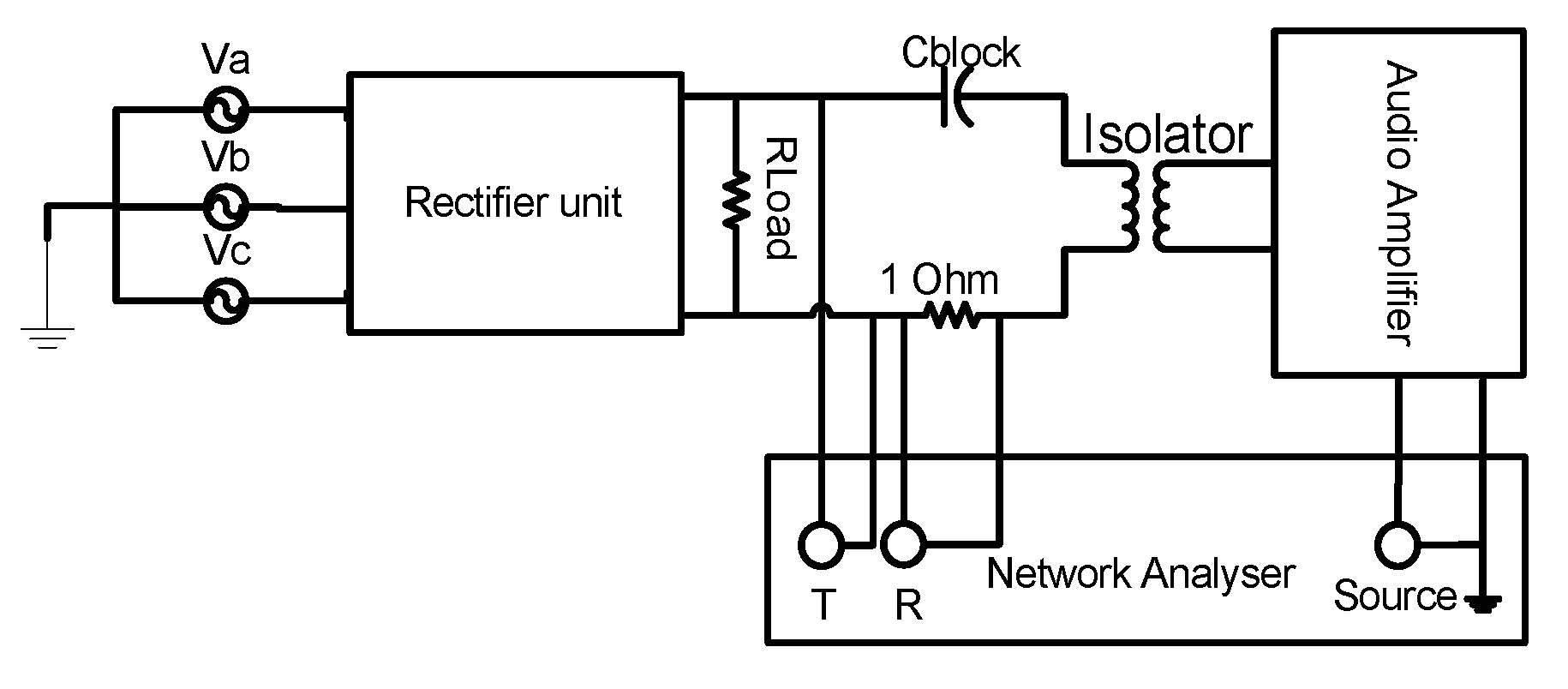
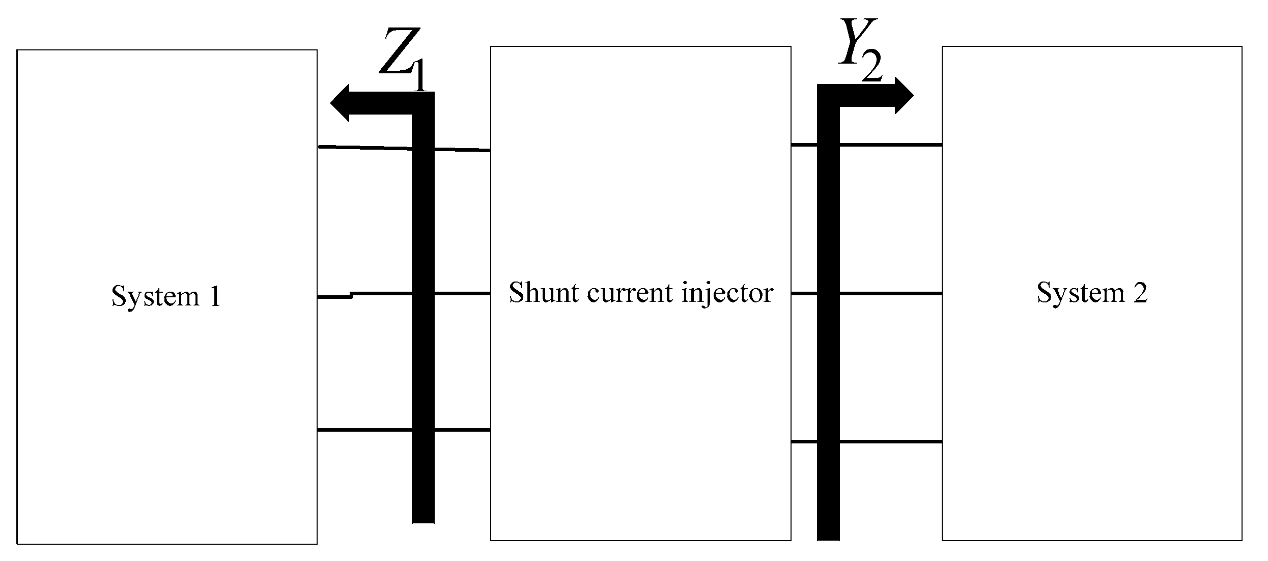
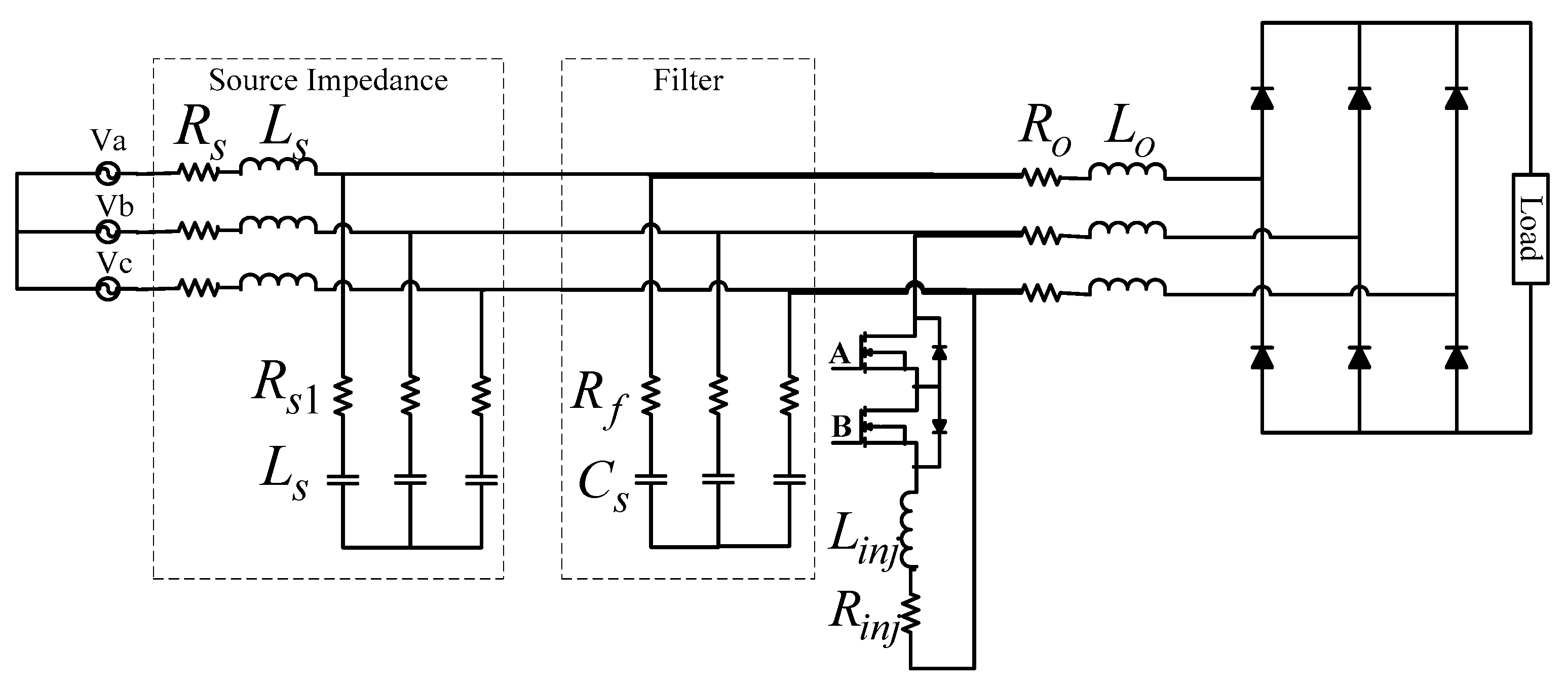
4. Experimental Setup for Impedance Measurements

4.1. DC Impedance Measurement

The Agilent Network analyzer (E5061B, Santa Clara, CA, USA), having a frequency range from 5 Hz to 3 GHz, was used for measuring the small signal output impedance. Circuit setup is shown in Figure 12 where 1 Ω resistor is used for sensing the current in the return path and a capacitor of a higher rating than that of the output voltage is used for blocking high DC voltage so as to protect the network analyzer from being damaged. Sweep frequency signal of 34 mV ranging from 10 Hz to 5 kHz was injected into the circuit through an amplifier and a small signal voltage and the current values were fed-back to the network analyzer through T and R terminals. Capacitor rated double that of operating load voltage was used for dc blocking. The current was measured using 1 Ω sense resistor as shown in Figure 12. Signal collected at T is divided by signal collected at R to obtain output impedance. This output impedance data, measured through impedance analyzer, was exported to MATLAB, identified into second order systems and redrawn for comparison with the output impedance obtained from derived average model as shown in Figure 13 and Figure 14.

4.2. AC Impedance Measurement

The four ac impedance terms$Z_{dd}$,$Z_{dq}$,$Z_{qd}$, and$Z_{qq}$described in Section 1, can be measured using Equations (43) and (44). For determining $Z_{qq}$ and $Z_{dq}$ at ${\omega }_p$, perturbation frequency is injected in $i_q$ while current $i_d$ is set to zero. However, for determining $Z_{dd}$ and$Z_{qd}$, perturbation frequency is injected in $i_d$ while$i_q$ is to be set to zero. This frequency response in the form of magnitude and phase is further identified into second order transfer functions which could be utilized for stability analysis using Nyquist criteria discussed in Section 1.

$$Z_{qq}\left({\omega }_p\right)=\frac{V_q}{i_q},i_d=0;Z_{dq}\left({\omega }_p\right)=\frac{V_d}{i_q},i_d=0;$$

(43)

$$Z_{dd}\left({\omega }_p\right)=\frac{V_d}{i_d},i_q=0;Z_{qd}\left({\omega }_p\right)=\frac{V_q}{i_q},i_q=0;$$

(44)

For switch model and experimental setup, an easy approach of using single line to line current injection technique is used for three phase ac impedance measurement. General diagram of ac impedance measurement technique is shown in Figure 15 while line to line current injection technique for three phase diode rectifier impedance measurement is shown in Figure 16. This technique is also applied to nine phase diode rectification system by measuring the ac impedance of each rectifier individually. Specifications for current injection setup with three phase diode rectifier system, are given in

Table 3. Circuit parameters.

No.	Parameter	Values
1	Power	2000 Watts
2	Line Frequency ($f_g)$	400 Hz
3	Input Voltage (Vg)	115 Vrms
4	$R_s$	10 mΩ
5	$L_s$	500 µH
6	$R_{s1}$	0.01 Ω
7	$C_s$	50 µF
8	$R_f$	10 mΩ
9	$C_f$	15 µF
10	$R_o$	40 mΩ
11	$L_o$	10 µH
12	$L_{inj}$	1 mH
13	$R_{inj}$	100 Ω
14	Load Resistance	30 Ω

. The chopper circuit, used for line to line shunt current injection, consists of a resistor and inductor in series with a bidirectional switch. Practically, line to line current is injected in any two of the three lines a, b and c by switching power MOSFETs (Motorola IRF 540, 150W, 27 Ampere, 100V) A and B alternatively, with 50% duty ratio, to introduce impedance variation at the interface junction. This causes current injection into system at the switching frequency. For calculating frequency response measurement at point${\omega }_p$, two linearly independent frequency signals are injected at$\omega =\left|{\omega }_p\pm {\omega }_g\right|$. Matlab script, based on flow chart as given in Figure 17, is used for transformation of ABC (three-axes coordinate system of ac voltages and currents) time domain values into DQ0 (two-axes coordinate system of ac voltages and currents) synchronous reference frame and then performing fast Fourier transform (FFT) to extract injected frequency dq values of voltage and current. Output impedance of system 1 and input admittance of system 2 can be calculated by utilizing Equations (45) and (46) but, only $Z_{dd}$ and $Z_{qq}$ impedances of these systems are extracted as shown in Figure 18, Figure 19, Figure 20, Figure 21 and Figure 22 respectively, for efficient utilization of space. These impedances are extracted from switch model as well as prototype using shunt current line to line injector circuit as shown in Figure 16. To avoid frequency overlapping, which may affect the results, multiples of fundamental frequency were not injected. This technique has a drawback of injecting considerable harmonics but they are mathematically removed by the FFT process.

$$\left[\begin{array}{c}d{v}_d\\ d{v}_q\end{array}\right]=\left[\begin{array}{cc}{Z}_{dd}& Z_{dq}\\ Z_{qd}& Z_{qq}\end{array}\right]\left[\begin{array}{c}d{i}_{ds}\\ d{i}_{qs}\end{array}\right]$$

(45)

$$\left[\begin{array}{c}d{i}_{dl}\\ d{i}_{ql}\end{array}\right]=\left[\begin{array}{cc}{Y}_{dd}& Y_{dq}\\ Y_{qd}& Y_{qq}\end{array}\right]\left[\begin{array}{c}d{v}_d\\ d{v}_q\end{array}\right]$$

(46)

5. Conclusions

With the addition of a linear variation term in the DC load current, it is evident from the results shown in the time domain and the frequency domain that there is a close resemblance, i.e., lower mean square error (MSE) with detailed model results. Similarly, increasing the order of equations further (adding quadratic term and higher) will fetch more improved results but the derivation will become more and more complex because of higher order derivative terms. Since the derived models are in close agreement with those of detailed models, the addition of higher terms to the dc load equation is exempted. To prove the validity and efficiency of derived average model, it is imperative to compare the results in time and frequency domain, under steady and dynamic states, with those of switching/detailed models/prototypes. The proposed average model is, therefore, compared in time domain and frequency domain, for three phase rectifier system as well as nine phase rectifier system shown in Section 3 and Section 4, which shows sufficiently close agreement with those of the detailed/switch model results hence proving the validity of the proposed AVMs. Steady and dynamic states of the systems can be observed from a single figure since it will reduce the space usage. Appropriate extraction of AC/DC impedances of integral parts of the interconnected systems is important since it has to deal with the stability analysis of the system. The proposed AVMs are much faster than switch model/detailed models.

References

1. Kulkarni, A.; Chen, W.; Bazzi, A. Implementation of Rapid Prototyping Tools for Power Loss and Cost Minimization of DC-DC Converters. Energies 2016, 9, 509. [Google Scholar] [CrossRef]
2. Kuo, M.; Tsou, M. Novel Frequency Swapping Technique for Conducted Electromagnetic Interference Suppression in Power Converter Applications. Energies 2017, 10, 24. [Google Scholar] [CrossRef]
3. Weilin, L.; Liliuyuan, L.; Wenjie, L.; Xiaohua, W. State of Charge Estimation of Lithium-Ion Batteries Using a Discrete-Time Nonlinear Observer. IEEE Trans. Ind. Electron. 2017, 64, 8557–8565. [Google Scholar]
4. Lee, K.; Venkataramanan, G.; Jahns, T.M. Source current harmonic analysis of adjustable speed drives under input voltage unbalance and sag conditions. IEEE Trans. Power Deliv. 2006, 21, 567–576. [Google Scholar] [CrossRef]
5. Lee, K.V.; Blasko, V.; Jahns, T.M.; Lipo, T.A. Input Harmonic Estimation and Control Methods in Active Rectifiers. IEEE Trans. Power Deliv. 2010, 25, 953–960. [Google Scholar] [CrossRef]
6. Villablanca, M.E.; Nadal, J.I. Current distortion reduction in six-phase parallel-connected AC/DC rectifiers. IEEE Trans. Power Deliv. 2008, 23, 953–959. [Google Scholar] [CrossRef]
7. Chiniforoosh, S.; Hamid, A.; Juri, J. A Generalized Methodology for Dynamic Average Modeling of High-Pulse-Count Rectifiers in Transient Simulation Programs. IEEE Trans. Energy Convers. 2016, 31, 228–239. [Google Scholar] [CrossRef]
8. Fangang, M.; Xiaona, X.; Lei, G. A Simple Harmonic Reduction Method in Multipulse Rectifier Using Passive Devices. IEEE Trans. Ind. Inform. 2017, 13, 2680–2692. [Google Scholar]
9. Mon-Nzongo, D.L.; Jin, T.; Ipoum-Ngome, P.G.; Song-Manguelle, J. An Improved Topology for Multipulse AC/DC Converters within HVDC and VFD Systems: Operation in Degraded Modes. IEEE Trans. Ind. Electron. 2018, 65, 3646–3656. [Google Scholar] [CrossRef]
10. Chiniforoosh, S.; Hamid, A.; Davoudi, A.; Jatskevich, J.; Martinez, J.A.; Saeedifard, M.; Aliprantis, D.C.; Sood, V.K. Steady-State and Dynamic Performance of Front-End Diode Rectifier Loads as Predicted by Dynamic Average-Value Models. IEEE Trans. Power Deliv. 2013, 28, 1533–1541. [Google Scholar] [CrossRef]
11. Yang, T.; Bozhko, S.; Le-Peuvedic, J.M.; Asher, G.; Hill, C.I. Dynamic Phasor Modeling of Multi-Generator Variable Frequency Electrical Power Systems. IEEE Trans. Power Syst. 2016, 31, 563–571. [Google Scholar] [CrossRef]
12. Chiniforoosh, S.; Jatskevich, J.; Dinavahi, V.; Iravani, R.; Martinez, J.A.; Ramirez, A. Dynamic average modeling of line-commutated converters for power systems applications. In Proceedings of the 2009 IEEE Power & Energy Society General Meeting, Calgary, AB, Canada, 26–30 July 2009. [Google Scholar]
13. Juan, A.; Martinez, V. Transient Analysis of Power Systems: Solution Techniques, Tools and Applications, 1st ed.; John Wiley & Sons, Ltd.: New York, NY, USA, 2015. [Google Scholar]
14. Chiniforoosh, S.; Jatskevich, J.; Yazdani, A.; Sood, V.; Dinavahi, V.; Martinez, J.A.; Ramirez, A. Definitions and applications of dynamic average models for analysis of power systems. IEEE Trans. Power Deliv. 2010, 25, 2655–2669. [Google Scholar] [CrossRef]
15. Shahbaz, K.; Zhang, X.; Husan, A.; Haider, Z.; Muhammad, S.; Bakht, M.K. Impedance extraction utilizing improved average models for three phase diode rectifiers. In Proceedings of the 2017 IEEE 3rd International Conference on Computer Science and System Engineering, Beijing, China, 17–19 August 2017. [Google Scholar]
16. Zhu, H. New Multipulse Diode Rectifier Average Models for AC and DC Power Systems Studies. Ph.D. Thesis, Virginia Polytechnic Institute, State University, Blacksburg, VA, USA, 2005. [Google Scholar]
17. Yang, T.; Bozhko, S.; Asher, G. Functional Modeling of Symmetrical Multipulse Autotransformer Rectifier Units for Aerospace Applications. IEEE Trans. Power Electron. 2015, 30, 4704–4713. [Google Scholar] [CrossRef]
18. Middlebrook, R.D. Input filter considerations in design and application of switching regulators. In Proceedings of the 1976 IEEE Industry Applications Annual Meeting, Chicago, IL, USA, 11–14 October 1976. [Google Scholar]
19. Panov, Y.; Jovanovic, M. Practical issues of input/output impedance measurements in switching power supplies and application of measured data to stability analysis. In Proceedings of the 20th Annual IEEE Applied Power Electronics Conference and Exposition, Austin, TX, USA, 6–8 March 2005. [Google Scholar]
20. Sanz, M.; Valdivia, V.; Zumel, P.; Moral, D.L.; Fernández, C.; Lázaro, A.; Barrado, A. Analysis of the Stability of Power Electronics Systems: A Practical Approach. In Proceedings of the 29th Annual IEEE Applied Power Electronics Conference and Exposition (APEC), Fort Worth, TX, USA, 16–20 March 2014. [Google Scholar]
21. Zheng, X.; Ali, H.; Wu, X.; Zaman, H.; Khan, S. Non-Linear Behavioral Modeling for DC-DC Converters and Dynamic Analysis of Distributed Energy Systems. Energies 2017, 10, 63. [Google Scholar] [CrossRef]
22. Huang, J.; Corzine, K.A.; Belkhayat, M. Small-Signal Impedance Measurement of Power-Electronics-Based AC Power Systems Using Line-to-Line Current Injection. IEEE Trans. Power Electron. 2009, 24, 445–455. [Google Scholar] [CrossRef]
23. Erickson, R.W.; Dragan, M. Fundamentals of Power Electronics, International Edition; Springer: Boulder, CO, USA, 2001. [Google Scholar]
24. Aldhaheri, A.; Etemadi, A. Impedance Decoupling in DC Distributed Systems to Maintain Stability and Dynamic Performance. Energies 2017, 10, 470. [Google Scholar] [CrossRef]
25. Simon, A.; Alejandro, O. Power-Switching Converters; Marcel Dekker, Inc.: New York, NY, USA, 1995. [Google Scholar]
26. Valerio, S.; Alessandro, C.; Stephen, M.C.; Pericle, Z. Stability Assessment of Power-Converter-Based AC systems by LTP Theory: Eigenvalue Analysis and Harmonic Impedance Estimation. IEEE J. Emerg. Sel. Top. Power Electron. 2017, 4, 1513–1525. [Google Scholar]
27. Bo, W.; Dushan, B.; Rolando, B.; Paolo, M.; Zhiyu, S. Analysis of D-Q Small-Signal Impedance of Grid-Tied Inverters. IEEE Trans. Power Electron. 2016, 31, 675–687. [Google Scholar]
28. Serrano-Finetti, R.E.; Pallas-Areny, R. Output impedance measurement in power sources and conditioners. In Proceedings of the 2007 IEEE Instrument and Measurement Technology Conference, Warsaw, Poland, 1–3 May 2007. [Google Scholar]
29. Cho, Y.; Hur, K.; Kang, Y.; Muljadi, E. Impedance-Based Stability Analysis in Grid Interconnection Impact Study Owing to the Increased Adoption of Converter-Interfaced Generators. Energies 2017, 10, 1355. [Google Scholar] [CrossRef]
30. Radwan, A.A.A.; Mohamed, Y.A.R.I. Assessment and Mitigation of Interaction Dynamics in Hybrid AC/DC Distribution Generation Systems. IEEE Trans. Smart Grid 2012, 3, 1382–1393. [Google Scholar] [CrossRef]
31. Xu, L.; Fan, L. Impedance-Based Resonance Analysis in a VSC-HVDC System. IEEE Trans. Power Deliv. 2013, 28, 2209–2216. [Google Scholar] [CrossRef]
32. Sun, J. Small-Signal Methods for AC Distributed Power Systems—A Review. IEEE Trans. Power Electron. 2009, 24, 2545–2554. [Google Scholar]
33. Sun, J. Impedance-Based Stability Criterion for Grid-Connected Inverters. IEEE Trans. Power Electron. 2011, 26, 3075–3078. [Google Scholar] [CrossRef]
34. Song, Y.; Wang, X.; Blaabjerg, F. Impedance-Based High-Frequency Resonance Analysis of DFIG System in Weak Grids. IEEE Trans. Power Electron. 2017, 32, 3536–3548. [Google Scholar] [CrossRef]
35. Cao, W.; Ma, Y.; Yang, L.; Wang, F.; Tolbert, L.M. D-Q Impedance Based Stability Analysis and Parameter. Design of Three-Phase Inverter-Based AC Power Systems. IEEE Trans. Ind. Electron. 2017, 64, 6017–6028. [Google Scholar] [CrossRef]
36. Cespedes, M.; Sun, J. Impedance Modeling and Analysis of Grid-Connected Voltage-Source Converters. IEEE Trans. Power Electron. 2014, 29, 1254–1261. [Google Scholar] [CrossRef]
37. Wen, B.; Dong, D.; Boroyevich, D.; Burgos, R.; Mattavelli, P.; Shen, Z. Impedance-Based Analysis of Grid-Synchronization Stability for Three-Phase Paralleled Converters. IEEE Trans. Power Electron. 2016, 31, 26–38. [Google Scholar] [CrossRef]
38. Wang, X.; Blaabjerg, F.; Wu, W. Modeling and Analysis of Harmonic Stability in an AC Power-Electronics-Based Power System. IEEE Trans. Power Electron. 2014, 29, 6421–6432. [Google Scholar] [CrossRef]
39. Lyu, J.; Cai, X.; Molinas, M. Frequency Domain Stability Analysis of MMC-Based HVDC for Wind Farm Integration. IEEE J. Emerg. Sel. Top. Power Electron. 2016, 4, 141–151. [Google Scholar] [CrossRef]
40. Bayo-Salas, A.; Beerten, J.; Rimez, J.; Hertem, D.V. Impedance-based stability assessment of parallel VSC HVDC grid connections. In Proceedings of the 11th IET International Conference on AC and DC Power Transmission, Birmingham, UK, 10–12 February 2015. [Google Scholar]
41. Wang, X.; Blaabjerg, F.; Liserre, M.; Chen, Z.; He, J.; Li, Y. An Active Damper for Stabilizing Power-Electronics-Based AC Systems. IEEE Trans. Power Electron. 2014, 29, 3318–3329. [Google Scholar] [CrossRef]
42. Shahbaz, K.; Zhang, X.; Husan, A.; Haider, Z.; Muhammad, S.; Bakht, M.K. AC impedance extraction for three phase systems. In Proceedings of the 2017 IEEE 3rd International Conference on Computer Science and System Engineering, Beijing, China, 17–19 August 2017. [Google Scholar]
43. Huang, J.; Corzine, K.A. Ac impedance measurement by line-to-line injected current. In Proceedings of the 41 IAS Annual Meeting of IEEE Conference on Industry Applications Conference, Tampa, FL, USA, 8–12 October 2006. [Google Scholar]
44. Liqiu, H.; Wang, J.; David, H. State-space average modelling of 6- and 12-pulse diode rectifiers. In Proceedings of the 2007 IEEE Conference on Power Electronics and Applications, Aalborg, Denmark, 2–5 September 2007. [Google Scholar]
45. Antonio, G.; Jiabin, W. State-space average modelling of synchronous generator fed 18-pulse diode rectifier. In Proceedings of the 2009 IEEE 13 Conference on Power Electronics and Applications, Barcelona, Spain, 8–10 September 2009. [Google Scholar]
Figure 1. Two systems interacting with each other.
Energies 11 00550 g001
Figure 2. Showing (a) commutation and (b) conduction periods in three phase rectifiers.
Energies 11 00550 g002
Figure 3. Waveforms showing commutation and conduction periods in three phase rectifiers.
Energies 11 00550 g003
Figure 4. Showing (a) commutation and (b) conduction periods in nine phase rectifiers.
Energies 11 00550 g004
Figure 5. Waveforms showing commutation and conduction periods in nine phase rectifiers.
Energies 11 00550 g005
Figure 6. Step change in the load voltage of a three phase rectifier for (a) average model vs. switch model and (b) average model vs. experimental.
Energies 11 00550 g006
Figure 7. Step change in the load current of a three phase rectifier (a) average model vs. switch model and (b) average model vs. experimental.
Energies 11 00550 g007
Figure 8. Step change in (a) average model vs switch model Id and Iq currents; (b) average model vs. experimental Id and (c) average model vs. experimental Iq.
Energies 11 00550 g008
Figure 9. Step change in the load voltage of a nine phase rectifier for (a) average model vs. switch model and (b) average model vs. experimental.
Energies 11 00550 g009
Figure 10. Step change in the load current of a nine phase rectifier for (a) average model vs. switch model and (b) average model vs. experimental.
Energies 11 00550 g010
Figure 11. Step change in Id and Iq currents of a nine phase rectifier for (a) average model vs. switch model and (b) average model vs. experimental.
Energies 11 00550 g011
Figure 12. Output impedance measurement setup.
Energies 11 00550 g012
Figure 13. Output impedance of (a) average model vs. switch model and (b) average vs. experimental of three phase rectifier.
Energies 11 00550 g013
Figure 14. Output impedance of (a) average model vs. switch model and (b) experimental (green and blue) vs. switch model (red asterisks) for nine-phase rectifier.
Energies 11 00550 g014
Figure 15. General diagram for line to line current injection.
Energies 11 00550 g015
Figure 16. Three phase diode rectifier impedance measurement setup.
Energies 11 00550 g016
Figure 17. Flow chart for impedance extraction Matlab code.
Energies 11 00550 g017
Figure 18. Three phase power supply ac output impedance (a) Zdd and (b) Zqq.
Energies 11 00550 g018
Figure 19. Switch model vs. average model ac input impedance (a) Zdd and (b) Zqq for three phase rectifier.
Energies 11 00550 g019
Figure 20. Experimental vs. average model ac input impedance (a) Zdd and (b) Zqq for three phase rectifier.
Energies 11 00550 g020
Figure 21. Switch model vs. average model ac input impedance (a) Zdd and (b) Zqq for nine phase rectifier.
Energies 11 00550 g021
Figure 22. Experimental vs. average model ac input impedance (a) Zdd and (b) Zqq for nine phase rectifier.
Energies 11 00550 g022