A Non-Probabilistic Solution for Uncertainty and Sensitivity Analysis on Techno-Economic Assessments of Biodiesel Production with Interval Uncertainties

Abstract

Techno-economic assessments (TEA) of biodiesel production may comply with various economic and technical uncertainties during the lifespan of the project, resulting in the variation of many parameters associated with biodiesel production, including price of biodiesel, feedstock price, and rate of interest. Engineers may only collect very limited information on these uncertain parameters such as their variation intervals with lower and upper bound. This paper proposes a novel non-probabilistic strategy for uncertainty analysis (UA) in the TEA of biodiesel production with interval parameters, and non-probabilistic reliability index (NPRI) is employed to measure the economically feasible extent of biodiesel production. A sensitivity analysis (SA) indicator is proposed to assess the sensitivity of NPRI with regard to an individual uncertain interval parameter. The optimization method is utilized to solve NPRI and SA. Results show that NPRI in the focused biodiesel production of interest is 0.1211, and price of biodiesel, price of feedstock, and cost of operating can considerably affect TEA of biodiesel production.

1. Introduction

The global climate, ecological environment, and air quality have been considerably affected by various deleterious emissions and harmful substances including NO_x, SO_x, CO₂, hydrocarbons, carbon monoxide, and particulate matter, resulting in various environmental pollution problems and danger on human health [1,2,3,4,5,6,7,8,9]. A great number of scientists are investigating other harmless, economic, and clean energy sources for the sake of the reduction of these adverse and negative effects. Being a valuable renewable energy resource, biodiesel is friendly to the natural environment and human health, compared to the traditional fossil fuels [10,11,12,13,14,15]. Various feedstocks-derived biodiesel production have been reported, for example, palm oil [16], waste cooking oil [17,18,19], vegetable oils [20,21], soybean oil [22,23,24,25], Jatropha curcas L. [26], algae [27,28], microalgae [28,29,30], Oleaginous yeast [31,32], lignocellulosic biomass [33], used frying oil [34], waste cottonseed oil with heterogeneous catalyst [35,36], Annona squamosa L. seed oil with heterogeneous catalyst [36,37], Butanol and pentanol [38], etc., and recent advances in biofeedstocks and biofuels have also been reviewed in [39].

Various uncertain factors existing in the biodiesel industry, such as fluctuation in interest rate, may cause instability in biodiesel production, and then may decrease the economical feasibility relevant to biodiesel production [40]. Numerous research works have investigated the techno-economic assessments (TEA) of biodiesel production to ensure the economical feasibility of biodiesel production [41,42,43,44,45,46,47,48,49,50,51], such as TEA for vegetable oil biodiesel production [41], TEA for palm biodiesel production [42], TEA for algal biofuel production [27,43,44,45], TEA for microalgae biofuel production [46,47], TEA for waste-to-biofuel production [48], TEA for sugarcane biorefineries [49], TEA for lignocellulosic biomass production [51], etc., and recent advances in TEA for biofuel production have also been summarized in [27,39,51]. These works have extensively improved the development in the TEA of biodiesel production on condition that all of the parameters relevant to the TEA are regarded as constant during the project’s lifespan. However, real engineering inevitably confronts various uncertain parameters resulting from numerous economic and technical uncertainties when performing TEA of biodiesel production [40], such as variation in the feedstock price [52], fluctuation of biodiesel price [52], and change in the rate of interest [53], and thus it may be more rational to treat these parameters as uncertain parameters. Recently, several works have studied the TEA of biodiesel production subject to many economic and technical uncertainties defined by random variables with probability density functions (PDFs) [54,55,56,57,58,59,60,61,62,63,64,65], including TEA for algae-derived biodiesel with uncertainties [55,56], TEA for biodiesel production with uncertainties using structural reliability principles [57], TEA for palm biodiesel production with uncertainties [58,59], TEA for inedible Jatropha oil biodiesel production with uncertainties [60], TEA for waste oil biodiesel production with uncertainties [61], probabilistic TEA for microalgae biofuel production [62], TEA for bioethanol production with uncertainties [63], stochastic TEA for alcohol-to-jet fuel production [64], TEA for high-value propylene glycol production with uncertainties [65], etc. These research works have discovered that the uncertainties related to the random parameters have distinct effects on the TEA. The authors also studied the TEA for palm biodiesel production with uncertainties, which were assumed as random variables with uniform distributions, indicating that uncertain parameters are uniformly distributed within variation intervals [58,59].

The previous studies [54,55,56,57,58,59,60,61,62,63,64,65] consider the effect of the uncertainties, and they consider the uncertainties as random variables following PDFs. Treating uncertainties as random variables may not be reasonable due to the fact that determining the precise PDFs requires a large number of data, but the data in practical engineering is usually limited due to lack of sufficient samples for TEA. This paper will propose a more rational solution for the TEA of palm biodiesel production based on the previous research works of the authors of [58,59]. In previous studies [58,59], the authors only collected very limited data on these uncertain parameters, and only the variation ranges or the lower bounds and upper bounds for uncertain parameters were determined. All of these uncertain parameters were assumed as random variables defined by uniform distributions, distributed uniformly within their variation ranges, and the TEA was done based on this assumption. The estimated results of the TEA may depend on the selected distributions for these uncertain parameters within their variation intervals, and different selection of distributions may lead to completely different estimated results. In order to overcome this difficulty, we will propose a more rational strategy for the TEA of a palm biodiesel production with interval parameters, in which only the lower limit and the upper limit of the parameters are available, being free from the selection of the distributions for uncertain parameters.

The rest of this paper is organized as follows. In Section 2, we propose a novel strategy for the evaluation of the TEA and sensitivity analysis (SA) for palm biodiesel production subject to interval uncertainties, specifically, non-probabilistic reliability index (NPRI) that measures the economically feasible extent of the biodiesel production and the effect of an interval parameter on NPRI. In Section 3, we evaluate the NPRI and SA associated with the TEA of the palm biodiesel production. In Section 4, we summarize our results and make some conclusions.

2. Materials and Methods

In this section, we first introduce several important indicators in the TEA of palm biodiesel production including net present value (NPV), payback period (PP), and total profit for this project, and then some important interval parameters related to the TEA are provided, which are determined by some collected data from some available references. Secondly, we introduce a novel indicator named as non-probabilistic reliability index to rationally measure the economically feasible degree of biodiesel production with interval uncertainties. Then, nonlinear optimization algorithm is employed to solve the NPRI in the TEA of palm biodiesel production. Finally, we develop a new sensitivity analysis (SA) indicator of NPRI with regard to an uncertain parameter, which can measure the effect of a parameter on NPRI and identify important parameters on the TEA.

2.1. Several Important Concepts in the TEA for a Biodiesel Production

We focus on the TEA for palm biodiesel production originally proposed in [42], in which economic and technical uncertainties are not considered. The mathematical formulations of total profit, payback period, and net present value for this problem are defined as [42,58,59]:

$$\begin{array}{ll}\mathrm{TotalProfit}& =-\mathrm{LCC}+\left(\mathrm{TBS}-\mathrm{TAX}\right)\times n=-\mathrm{LCC}+\left(\mathrm{TBS}-\mathrm{TAX}\right)\times 20\\ & =\left({\mathrm{TBS}}_i-{\mathrm{TAX}}_i\right)\times 20-\mathrm{LCC}\end{array}$$

(1)

$$\mathrm{PP}=\frac{\mathrm{CC}}{\left(\mathrm{TotalProfit}/n\right)}=\frac{n\times \mathrm{CC}}{\mathrm{TotalProfit}}$$

(2)

$$\begin{array}{l}\mathrm{NPV}={\displaystyle \sum _{i=1}^n\frac{\left({\mathrm{TBS}}_i-{\mathrm{TAX}}_i\right)}{{\left(1+r\right)}^i}}-\mathrm{LCC}\\ =-\mathrm{LCC}+{\displaystyle \sum _{i=1}^n\frac{\left(\mathrm{TBS}-\mathrm{TAX}\right)}{{\left(1+r\right)}^i}}=-\mathrm{LCC}+{\displaystyle \sum _{i=1}^n\frac{\mathrm{TotalProfit}+\mathrm{LCC}}{n{\left(1+r\right)}^i}}\\ =-\mathrm{LCC}+\frac{\mathrm{TotalProfit}+\mathrm{LCC}}{n}{\displaystyle \sum _{i=1}^n\frac{1}{{\left(1+r\right)}^i}}.\end{array}$$

(3)

with

$$\begin{array}{ll}\mathrm{LCC}& =\mathrm{CC}+\mathrm{MC}+\mathrm{FC}+\mathrm{OC}-\mathrm{BPC}-\mathrm{SV}\\ & =\mathrm{CC}+{\displaystyle \sum _{i=1}^n\frac{{\mathrm{FC}}_i+{\mathrm{OC}}_i+{\mathrm{MC}}_i}{{\left(1+r\right)}^i}}-\frac{\mathrm{SV}}{{\left(1+r\right)}^n}-{\displaystyle \sum _{i=1}^n\frac{{\mathrm{BPC}}_i}{{\left(1+r\right)}^i}}\end{array}$$

(4)

where TotalProfit is total profit of the project, PP is payback period, and NPV represents net present value; MC, CC, FC, LCC, OC, BPC, and SV represent maintenance cost, capital cost, feedstock cost, life cycle cost, operating cost, byproduct credit, and salvage value indicating the remaining value of the components and the assets of the plant at the end of the project’s lifetime, respectively; TBS is annual total biodiesel sale, TAX is annual total taxation, n = 22 years is project’s lifetime, and r represents rate of interest which takes values from 4.44% to 13.53% [66], i.e., $r\in \left[4.44\%,13.53\%\right]$; MC_i, FC_i, OC_i, BPC_i, TAX_i and TBS_i are maintenance cost, feedstock cost, operating cost, byproduct credit, total taxation, and total biodiesel sale for the ith year, respectively.

The annual production capacity for this plant is 50 kt, that is, PC = 50 kt, and its capital cost should take values between $9 million and $15 million, that is, $\mathrm{CC}\in \left[\$9\mathrm{million},\$15\mathrm{million}\right]$ [42]. The corresponding FC, OC, MC, SV, BPC, TBS, and TAX are defined by:

$$\mathrm{FC}={\displaystyle \sum _{i=1}^n{\mathrm{FC}}_i}={\displaystyle \sum _{i=1}^n\frac{\mathrm{FP}\times \mathrm{FU}}{{\left(1+r\right)}^i}}={\displaystyle \sum _{i=1}^n\frac{\mathrm{FP}\times \frac{\mathrm{PC}\times 1000}{\mathrm{CE}}}{{\left(1+r\right)}^i}}$$

(5)

$$\mathrm{OC}={\displaystyle \sum _{i=1}^n{\mathrm{OC}}_i}={\displaystyle \sum _{i=1}^n\frac{\mathrm{OR}\times \mathrm{PC}\times 1000}{{\left(1+r\right)}^i}}$$

(6)

$$\mathrm{MC}={\displaystyle \sum _{i=1}^n{\mathrm{MC}}_i}={\displaystyle \sum _{i=1}^n\frac{\mathrm{MR}\times \mathrm{CC}}{{\left(1+r\right)}^i}}$$

(7)

$$\mathrm{SV}=\mathrm{RC}\times {\left(1-d\right)}^{n-1}\times {\mathrm{PWF}}_n=\frac{\mathrm{RC}\times {\left(1-d\right)}^{n-1}}{{\left(1+r\right)}^n}$$

(8)

$$\mathrm{BPC}={\displaystyle \sum _{i=1}^n{\mathrm{BPC}}_i}={\displaystyle \sum _{i=1}^n\frac{\mathrm{GP}\times \mathrm{GCF}\times \mathrm{PC}\times {10}^6}{{\left(1+r\right)}^i}}$$

(9)

$$\mathrm{TBS}=\mathrm{PC}\times {10}^6/\rho \times \mathrm{BP}$$

(10)

$$\mathrm{TAX}=\mathrm{TBS}\times \mathrm{TR}$$

(11)

where FC commonly makes up about 80–90% of life cycle cost [67], and OC generally accounts for not more than 15% of life cycle cost [68]; FP is feedstock price or crude palm oil price, which takes values between $200/t and $1200/t in the past years [42], that is, $\mathrm{FP}\in \left[\$200/\mathrm{t},\$1200/\mathrm{t}\right]$; FU is annual total feedstock consumption; CE is conversion efficiency from palm oil to biodiesel which commonly takes values between 96% and 99% [69], that is, $\mathrm{CE}\in \left[96\%,99\%\right]$; OR is the operating rate, indicating operating cost of per-ton biodiesel production, which varies from $37.5/t to $225/t evaluated by feedstock price $\mathrm{FP}\in \left[\$200/\mathrm{t},\$1200/\mathrm{t}\right]$ [42] when FC makes up 80% of life cycle cost [67] and OC accounts for 15% of life cycle cost [68], that is, $\mathrm{OR}\in \left[\$37.5/\mathrm{t},\$225/\mathrm{t}\right]$; MR is maintenance rate, varying from 1% to 2%, i.e., $\mathrm{MR}\in \left[1\%,2\%\right]$ [41,42]; d and RC represent depreciation rate and replacement cost respectively, that is, RC = $10 million and d = 5% [42]; GP and GCF represent glycerol price and glycerol conversion factor, that is, $\mathrm{GP}\in \left[\$0.08/\mathrm{kg},\$0.2/\mathrm{kg}\right]$ [70] and GCF = 0.0985 [42]; BP is biodiesel price, that is, $\mathrm{BP}\in \left[\$0.66/\mathrm{L},\$1.58/\mathrm{L}\right]$ [71]; ρ is biodiesel density, i.e., ρ = 0.95 kg/L; and TR = 15% is tax rate for biodiesel sale.

The important quantities involved in the TEA, such as life cycle cost, net present value, payback period, and total profit, unavoidably meet with various economic and technical uncertainties within the project lifespan.

Table 1. Variation intervals of uncertain parameters for biodiesel production.

Uncertain Parameters	Variation Intervals [${\underset{\mathbf{¯}}{\mathit{x}}}_{\mathit{i}}$, ${\overline{\mathit{x}}}_{\mathit{i}}$]
Capital cost (CC: $x_1$) [42]	[$9 million, $15 million]
Interest rate (r: $x_2$) [66]	[4.44%, 13.53%]
Operating rate (OR: $x_3$) [42,67,68]	[$37.5/t, $225/t]
Feedstock price (FP: $x_4$) [42]	[$200/t, $1200/t]
Glycerol price (GP: $x_5$) [70]	[$0.08/kg, $0.2/kg]
Maintenance rate (MR: $x_6$) [41,42]	[1%, 2%]
Biodiesel conversion efficiency (CE: $x_7$) [69]	[96%, 99%]
Biodiesel price (BP: $x_8$) [71]	[$0.66/L, $1.58/L]

gives the variation intervals for these uncertain parameters, which are obtained by the collected data from many available research works.

2.2. NPRI for Measuring Economically Feasible Extent of Biodiesel Production

In this section, we will first introduce a NPRI, which is commonly employed to measure the reliable level of practical engineering problems subject to interval uncertainties. Then, NPRI is further extended to measure the economically feasible degree in the TEA of biodiesel production.

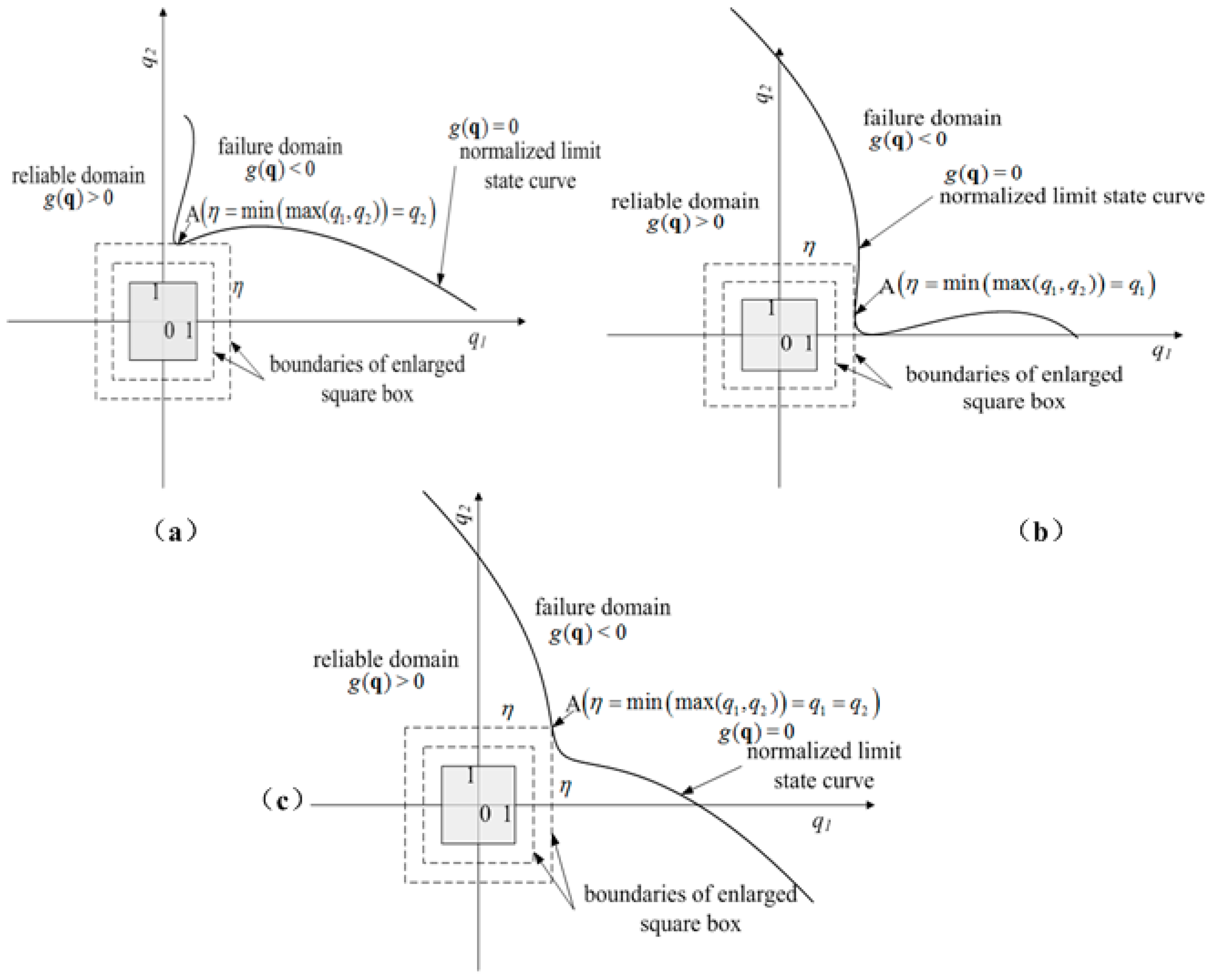
2.2.1. NPRI for Problems with Interval Parameters

For a system with interval input parameters $\mathit{x}=\left(x_1,x_2,\dots ,x_n\right)$, the corresponding output $y$ is defined by:

$$y=g\left(\mathit{x}\right)$$

(12)

where $\mathit{x}$ represents the input parameters with interval uncertainties, and $y$ commonly is the continuous function of the inputs $\mathit{x}=\left(x_1,x_2,\dots ,x_n\right)$. Obviously, $y$ varies within an interval with a lower bound $\underset{¯}{y}$ and an upper bound $\overline{y}$. In general, ${\Omega }_s=\left\{\mathit{x}|y=g\left(\mathit{x}\right)\ge 0;\mathit{x}=\left(x_1,x_2,\dots ,x_n\right)\right\}$ indicates the safe region, and ${\Omega }_f=\left\{\mathit{x}|y=g\left(\mathit{x}\right)<0;\mathit{x}=\left(x_1,x_2,\dots ,x_n\right)\right\}$ represents the failure region. In addition, $y=g\left(\mathit{x}\right)=0$ is named as limit state function (LSF) or limit state curve (LSC), separating the whole space into two regions, that is, the safe region and failure region. Non-probabilistic reliability index has been employed for measuring the reliable level related to the system with interval parameters as [72,73,74,75]:

$$\eta =y^c/y^r$$

(13)

with

$$y^c=\left(\overline{y}+\underset{¯}{y}\right)/2$$

and

$$y^r=\left(\overline{y}-\underset{¯}{y}\right)/2$$

where $\eta$ is NPRI; $\underset{¯}{y}$ and $\overline{y}$ are lower limit and upper limit of the output $y$. When $\eta \ge 1$ holds, one can have $\underset{¯}{y}\ge 0$ holds, indicating that the output is always larger than or equals to zero and thus the system is absolutely safe. Condition $\eta \le -1$ will lead to $\overline{y}\le 0$, implying that the system is completely a failure. Accordingly, $-1<\eta <1$ corresponds to $\underset{¯}{y}<0<\overline{y}$, which indicates that a part of the output will lie in the failure space and the system is not reliable. Thus, $\eta$ can be employed to measure the reliable degree associated with a system with interval uncertainties, and a larger value of $\eta$ corresponds to a more reliable system and vice versa [72,73,74,75]. In general, engineers focus on the situation with $\eta \ge 0$. The following will further discuss the physical significance in the NPRI.

For $x_i$, we first do the following standard transformation [72,73,74,75]:

$$x_i=x_i^c+x_i^r{q}_i=\frac{\left({\overline{x}}_i-{\underset{¯}{x}}_i\right)}{2}{q}_i+\frac{\left({\overline{x}}_i+{\underset{¯}{x}}_i\right)}{2}$$

(14)

where $q_i\in \left[-1,1\right]$ is the normalized interval for $x_i$. Substituting Equation (14) into Equation (12) can lead to normalized formulation for $y$ as

$$y=g\left(\mathbf{q}\right)=g\left(q_1,q_2,\dots ,q_n\right)$$

(15)

Obviously, the normalized intervals $\mathbf{q}$ of Equation (15) vary in the domain ${\Omega }_{\mathbf{q}}=\left\{\mathbf{q}|\left|q_i\right|\le 1;i=1,2,\dots ,n\right\}$, which is a hyperbox. Figure 1 illustrates the representative figure of ${\Omega }_{\mathbf{q}}$ in a two-dimension situation, in which ${\Omega }_{\mathbf{q}}$ is a square centered at coordinate origin and its side-length is 2, representing the set consisting of all the possible values of the two normalized intervals. When the square box enlarges proportionally in two directions, all the possible values of the two interval variables will locate in the reliable domain until the square box is tangential to normalized LSC $y=g\left(\mathbf{q}\right)=0$. The maximum allowable variability can be defined by the shortest distance between LSC $y=g\left(\mathbf{q}\right)=0$ and the coordinate origin in the normalized space in the form of infinite norm [72,73,74,75], which can be employed to measure the reliable extent of the system, i.e., non-probabilistic reliability index. More discussions on non-probabilistic reliability can be found in [76,77,78,79,80,81].

According to the discussion in Figure 1, another mathematical definition of NPRI $\eta$ can be provided by [72,73,74,75]:

$$\begin{array}{l}\eta =\min \left({\Vert \mathbf{q}\Vert }_{\infty }\right)\\ \mathrm{S}.\mathrm{t}.g\left(\mathbf{q}\right)=g\left(q_1,q_2,\dots ,q_n\right)=0\end{array}$$

(16)

with

$${\Vert \mathbf{q}\Vert }_{\infty }=\max \left(\left|q_1\right|,\left|q_2\right|,\dots ,\left|q_n\right|\right)$$

where $\min (•)$ is the operation of taking the minimum of the set, ${\Vert •\Vert }_{\infty }$ represents the operation of infinite norm, $\max (•)$ is the operation of taking the maximum of the set, and $|•|$ denotes the operation of taking the absolute value. If a system has m outputs $y_j=g_j\left(\mathit{x}\right)\left(j=1,2,\dots ,m\right)$ which corresponds to m failure modes, then failure associated with anyone of them will lead to the failure of the whole system. Thus, NPRI ${\eta }_s$ for system is provided as:

$${\eta }_s=\min \left\{{\eta }_1,{\eta }_2,\dots ,{\eta }_m\right\}$$

(17)

where ${\eta }_j\left(j=1,2,\dots ,m\right)$ is NPRI associated with $y_j=g_j\left(\mathit{x}\right)\left(j=1,2,\dots ,m\right)$.

2.2.2. NPRI for Economically Feasible Degree in the TEA of Biodiesel Production

Total profit defined in Equation (1) is expected to be larger than zero, specifically,

$$\mathrm{TotalProfit}\ge 0.$$

(18)

Meanwhile, payback period given in Equation (2) is expected to be less than the allowable upper bound, that is,

$$\mathrm{PP}=\frac{\mathrm{CC}}{\left(\mathrm{TotalProfit}/n\right)}=\frac{n\times \mathrm{CC}}{\mathrm{TotalProfit}}\le {\mathrm{PP}}^u.$$

(19)

where ${\mathrm{PP}}^u$ is the permitted upper limit, and here ${\mathrm{PP}}^u$ is one third of project’s lifespan, that is, ${\mathrm{PP}}^u=n/3=20/3$ years. Then, Equation (19) is transformed into Equation (20):

$$\frac{n\times \mathrm{CC}}{\mathrm{TotalProfit}}\le {\mathrm{PP}}^u\Rightarrow \mathrm{TotalProfit}\ge \frac{n\times \mathrm{CC}}{{\mathrm{PP}}^u}.$$

(20)

Finally, NPV given by Equation (3) must be larger than zero, specifically,

$$\mathrm{NPV}=-\mathrm{LCC}+\frac{\mathrm{TotalProfit}+\mathrm{LCC}}{n}{\displaystyle \sum _{i=1}^n\frac{1}{{\left(1+r\right)}^i}}\ge 0.$$

(21)

Then, Equation (21) can be transformed into Equation (22):

$$\mathrm{TotalProfit}\ge \left(\frac{n}{{\displaystyle \sum _{i=1}^n\frac{1}{{\left(1+r\right)}^i}}}-1\right)\times \mathrm{LCC}.$$

(22)

Thus, Equations (18), (20), and (22) should simultaneously hold to ensure that biodiesel production is economically feasible. For the sake of convenience, Equations (18), (20), and (22) can be written into the following forms:

$$y_1=g_1\left(\mathit{x}\right)=\mathrm{TotalProfit}$$

(23)

$$y_2=g_2\left(\mathit{x}\right)=\mathrm{TotalProfit}-\frac{n\times \mathrm{CC}}{{\mathrm{PP}}^u}$$

(24)

$$y_3=g_3\left(\mathit{x}\right)=\mathrm{TotalProfit}-\left(\frac{n}{{\displaystyle \sum _{i=1}^n\frac{1}{{\left(1+r\right)}^i}}}-1\right)\times \mathrm{LCC}$$

(25)

where $y_1=g_1\left(\mathit{x}\right)$, $y_2=g_2\left(\mathit{x}\right)$, and $y_3=g_3\left(\mathit{x}\right)$ are LSFs, and $\mathit{x}$ represents the vector consisting of interval parameters, as shown in Table 1.

Uncertainties involved in the interval parameters in Table 1 will lead to the variability of the TotalProfit, payback period, and NPV defined in Equations (1)–(3), and then one, two, or all of Equations (23)–(25) may not hold. Any one of the three LSFs in Equations (23)–(25) not being feasible will lead to the result that biodiesel production will not be economically feasible. In other words, biodiesel production is economically feasible if and only if the three LSFs in Equations (23)–(25) simultaneously apply. Thus, according to Equation (17), the following indicator can be employed to measure the economically feasible degree of biodiesel production with interval parameters:

$${\eta }_s=\min \left\{{\eta }_1,{\eta }_2,{\eta }_3\right\}$$

(26)

where ${\eta }_s$ represents NPRI for measuring economical feasibility of biodiesel production; ${\eta }_j\left(j=1,2,3\right)$ is NPRI for $y_j=g_j\left(\mathit{x}\right)$ given in Equations (23)–(25). The significance relevant to ${\eta }_s$ will be discussed in the following.

When ${\eta }_s\ge 1$ holds, the minimum of ${\eta }_1$, ${\eta }_2$, and ${\eta }_3$ will be larger than or equal to one, then ${\underset{¯}{y}}_1\ge 0$, ${\underset{¯}{y}}_2\ge 0$, and ${\underset{¯}{y}}_3\ge 0$ in Equations (23)–(25) hold, indicating biodiesel production with interval uncertainties is absolutely feasible in terms of economical feasibility. When $0<{\eta }_s<1$ holds, the minimum of ${\eta }_1$, ${\eta }_2$, and ${\eta }_3$ will be less than one, then ${\overline{y}}_1\ge 0$, ${\overline{y}}_2\ge 0$, and ${\overline{y}}_3\ge 0$ hold, while at least one of ${\underset{¯}{y}}_1<0$, ${\underset{¯}{y}}_2<0$, and ${\underset{¯}{y}}_3<0$ holds, implying that biodiesel production with interval uncertainties is partially feasible. When ${\eta }_s<0$ holds, the minimum of ${\eta }_1$, ${\eta }_2$, and ${\eta }_3$ will be less than 0, and at least one of ${\overline{y}}_1<0$, ${\overline{y}}_2<0$, and ${\overline{y}}_3<0$ holds, indicating that biodiesel production with interval uncertainties is completely infeasible. Thus, ${\eta }_s$ can be employed to measure the economical feasibility relevant to biodiesel production with interval uncertainties, and a larger value of ${\eta }_s$ corresponds to a better economical feasibility of biodiesel production with interval uncertainties and vice versa.

2.3. Evaluation Procedure of the NPRI

According to the definition of NPRI in Equation (13), we need to first evaluate ${\underset{¯}{y}}_j$ and ${\overline{y}}_j$ for the evaluation of ${\eta }_j\left(j=1,2,3\right)$ for Equations (23)–(25). The following two equations can be utilized to calculate ${\underset{¯}{y}}_j$ and ${\overline{y}}_j$ as:

$$\begin{array}{cc}\hfill {\underset{¯}{y}}_j& =\underset{\mathit{x}}{\min }{g}_j\left(\mathit{x}\right)\hfill \\ \hfill \mathrm{S}.\mathrm{t}.& {\underset{¯}{x}}_i\le x_i\le {\overline{x}}_i\hfill \\ & \mathit{x}=\left(x_1,x_2,\dots ,x_8\right)\hfill \\ & j=1,2,3\hfill \\ & i=1,2,\dots ,8\hfill \end{array}$$

(27)

and

$$\begin{array}{cc}\hfill {\overline{y}}_j& =\underset{\mathit{x}}{\max }{g}_j\left(\mathit{x}\right)\hfill \\ \hfill \mathrm{S}.\mathrm{t}.& {\underset{¯}{x}}_i\le x_i\le {\overline{x}}_i\hfill \\ & \mathit{x}=\left(x_1,x_2,\dots ,x_8\right)\hfill \\ & j=1,2,3\hfill \\ & i=1,2,\dots ,8\hfill \end{array}$$

(28)

In this paper, an available optimization function of Matlab, i.e., fmincon, is employed to evaluate ${\underset{¯}{y}}_j$ and ${\overline{y}}_j$ defined in Equations (27) and (28), then NPRI ${\eta }_j\left(j=1,2,3\right)$ for Equations (23)–(25) can be estimated, and NPRI ${\eta }_s$ for measuring economical feasibility of biodiesel production with interval uncertainties can be calculated by Equation (26).

2.4. SA of NPRI for Economical Feasibility of Biodiesel Production with Regards to Uncertain Interval Parameter

When an interval parameter $x_i\left(i=1,2,\dots ,8\right)$ is fixed at $x_{ij}\in \left[{\underset{¯}{x}}_i,{\overline{x}}_i\right]\left(j=1,2,\dots ,p\right)$, i.e., $x_i=x_{ij}$, indicating that $x_i$ takes a value within the lower bound ${\underset{¯}{x}}_i$ and the upper bound ${\overline{x}}_i$, the uncertainty associated with $x_i$ is eliminated, and original NPRI ${\eta }_s$ will become ${\eta }_{s|x_i=x_{ij}}$. The absolute difference $\Delta {\eta }_{s|x_i=x_{ij}}$ between original NPRI ${\eta }_s$ and ${\eta }_{s|x_i=x_{ij}}$ can reflect the effect of the elimination of uncertainty related to $x_i$, which can be defined by:

$$\Delta {\eta }_{s|x_i=x_{ij}}=\left|{\eta }_s-{\eta }_{s|x_i=x_{ij}}\right|\left(j=1,2,\dots ,p\right),$$

(29)

where ${\eta }_{s|x_i=x_{ij}}$ can be evaluated by the method given in Section 2.3, similar to the evaluation procedure for ${\eta }_s$. When $x_i\left(i=1,2,\dots ,8\right)$ takes different values, i.e., $x_{i1},x_{i2},\dots ,x_{ip}$, the original NPRI ${\eta }_s$ will become ${\eta }_{s|x_i=x_{i1}},{\eta }_{s|x_i=x_{i2}},\dots ,{\eta }_{s|x_i=x_{ip}}$, and then $p$ absolute differences can be obtained by Equation (29), i.e., $\Delta {\eta }_{s|x_i=x_{i1}},\Delta {\eta }_{s|x_i=x_{i2}},\dots ,\Delta {\eta }_{s|x_i=x_{ip}}$. The average of the $p$ absolute differences, i.e., $\Delta {\eta }_{s|x_i=x_{i1}},\Delta {\eta }_{s|x_i=x_{i2}},\dots ,\Delta {\eta }_{s|x_i=x_{ip}}$, can be employed to define the sensitivity of NPRI with regards to $x_i$, which can measure the effect of $x_i$ on NPRI:

$${\mathrm{IM}}_i=\frac{1}{p}{\displaystyle \sum _{j=1}^p\Delta {\eta }_{s|x_i=x_{ij}}}\left(j=1,2,\dots ,p\right)$$

(30)

where ${\mathrm{IM}}_i$ represents the average shift in the NPRI due to the elimination of uncertainty in $x_i$.

Similar to ${\mathrm{IM}}_i$, the average difference rate in the NPRI because of eliminating uncertainty associated with $x_i$ can be defined as:

$${\mathrm{IMR}}_i=\frac{1}{p}{\displaystyle \sum _{j=1}^p\Delta \eta R_{s|x_i=x_{ij}}}\left(j=1,2,\dots ,p\right)$$

(31)

with

$$\Delta \eta R_{s|x_i=x_{ij}}=\frac{\left|{\eta }_s-{\eta }_{s|x_i=x_{ij}}\right|}{{\eta }_s}\left(j=1,2,\dots ,p\right)$$

(32)

where $\Delta \eta R_{s|x_i=x_{ij}}$ measures the absolute difference rate between ${\eta }_s$ and ${\eta }_{s|x_i=x_{ij}}$ with regard to ${\eta }_s$ when $x_i=x_{ij}$ ($x_{ij}\in \left[{\underset{¯}{x}}_i,{\overline{x}}_i\right]$).

The important interval parameters and non-important ones can be identified by the values of ${\mathrm{IM}}_i$ and ${\mathrm{IMR}}_i$. An interval parameter with large values of ${\mathrm{IM}}_i$ and ${\mathrm{IMR}}_i$ belongs to the important interval parameters, while one with small values of ${\mathrm{IM}}_i$ and ${\mathrm{IMR}}_i$ is considered as the non-important parameters. If $x_i$ has small values for ${\mathrm{IM}}_i$ and ${\mathrm{IMR}}_i$, $x_i$ can be fixed to any value within its variation interval, which will not considerably affect NPRI ${\eta }_s$.

3. Results and Discussion

In this section, we first evaluate NPRI ${\eta }_s$ for biodiesel production with the eight interval parameters shown in Table 1. Then, the corresponding sensitivity analysis of NPRI ${\eta }_s$ with regard to interval parameter $x_i$, i.e., ${\mathrm{IM}}_i$ and ${\mathrm{IMR}}_i$, is estimated. Finally, the interval parameters are classified into the important ones and non-important ones by the size of the values of ${\mathrm{IM}}_i$ and ${\mathrm{IMR}}_i$.

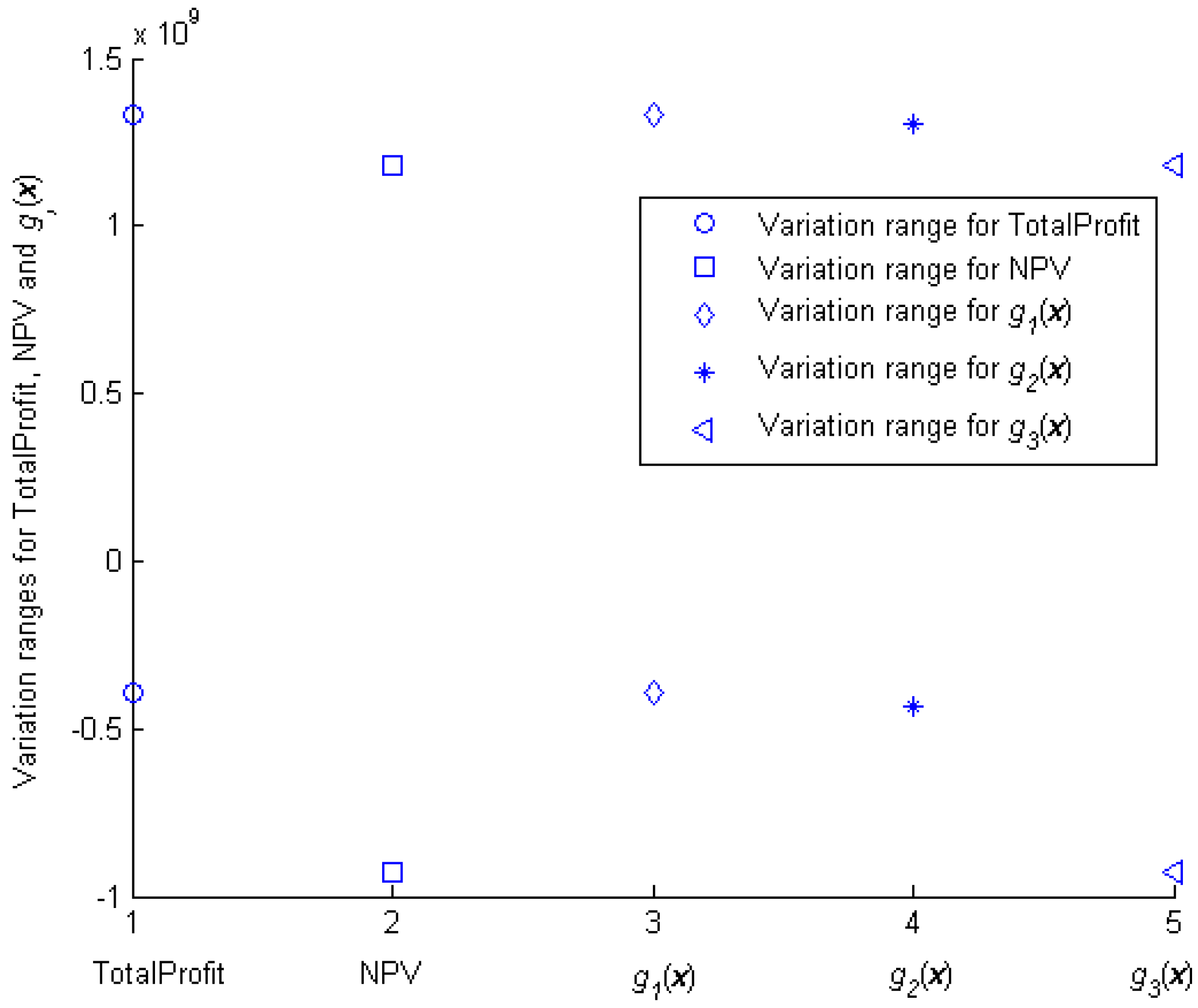
3.1. Evaluation of NPRI for Biodiesel Production

Biodiesel production has eight interval parameters because of economic and technical uncertainties when performing techno-economic assessments, and all interval parameters have been summarized in Table 1. The uncertainty in these interval parameters will result in the variation of the total profit, net present value, and payback period of biodiesel production. Figure 2 has shown the variation intervals for total profit (USD) expressed in Equation (1), net present value (USD) formulated in Equation (3), and $y_j=g_j\left(\mathit{x}\right)$ given in Equations (23)–(25). Two important observations have been revealed in Figure 2. The first observation is that total profit, net present value, and $y_j=g_j\left(\mathit{x}\right)\left(j=1,2,3\right)$ have exhibited variability owing to the effect of the uncertainties related to the interval parameters, i.e., $\mathrm{TotalProfit}\in \left[-3.8935\times {10}^8,1.3296\times {10}^9\right]$, $\mathrm{NPV}\in \left[-9.2579\times {10}^8,1.1808\times {10}^9\right]$, $y_1=g_1\left(\mathit{x}\right)\in \left[-3.8935\times {10}^8,1.3296\times {10}^9\right]$, $y_2=g_2\left(\mathit{x}\right)\in \left[-4.3435\times {10}^8,1.3026\times {10}^9\right]$, and $y_3=g_3\left(\mathit{x}\right)\in \left[-9.2579\times {10}^8,1.1808\times {10}^9\right]$. Secondly, we can find that a part of total profit, net present value, and $y_j=g_j\left(\mathit{x}\right)$ have been less than zero because of the effect of the uncertainty in these interval parameters, implying that biodiesel production is partially economically feasible, and has the possibility of being infeasible in the presence of the economic and technical uncertainties.

Figure 2 depicts the variation intervals of $y_j=g_j\left(\mathit{x}\right)\left(j=1,2,3\right)$, including lower limit ${\underset{¯}{y}}_j$ and upper limit ${\overline{y}}_j$ for three LSFs defined in Equations (23)–(25). Substituting ${\underset{¯}{y}}_j$ and ${\overline{y}}_j$ into Equation (15) leads to NPRI ${\eta }_j\left(j=1,2,3\right)$ of Equations (23)–(25). Finally, the estimated value of NPRI can be obtained as 1.2104 × 10⁻¹ by using Equation (26). A value of 1.2104 × 10⁻¹ for ${\eta }_s$ implies that the project will not be profitable to a great extent, in other words, a considerable part of the outcomes may be economically infeasible under the uncertain interval parameters shown in Table 1.

In our previous work [59], all the uncertain parameters are assumed as random variables following uniform distributions within their ranges, and we propose economical infeasibility probability (EIP) to measure economical feasibility for biodiesel production. For the same problem, the estimated value for EIP is 0.3676, implying that the project is partially economically feasible and the plant may be profitable with the probability of 0.6324, and in other words, 63.24 out of 100 outcomes will be economically feasible under the assumed probabilistic distribution [59]. Here, we perform the TEA in terms of the non-probabilistic perspective being free from the probabilistic distribution assumption, and the estimated result for NPRI is 1.2104 × 10⁻¹, also indicating that the project is partially economically feasible, according to the discussion in Section 2.2. Thus, the two methods have the same decisions. It is noted that the introduced method in this work is more rational than that in the previous work [59], which is subjected to the assumption on probabilistic distribution and different assumptions can lead to different results for EIP.

The previous results reveal that interval parameters resulting from uncertainties can remarkably affect the TEA of biodiesel production. We will further quantify the effect of an interval uncertain parameter on the economical feasibility by the sensitivity analysis proposed in Section 2.4.

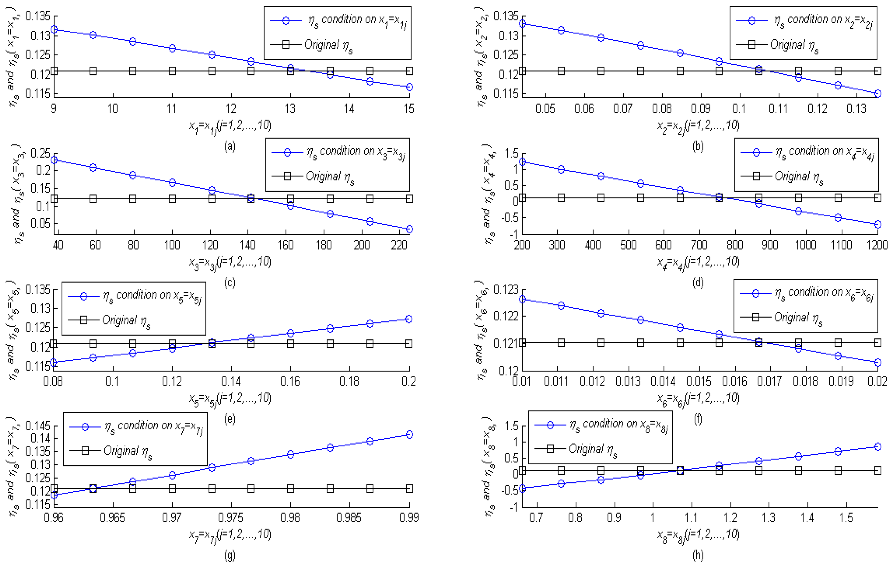
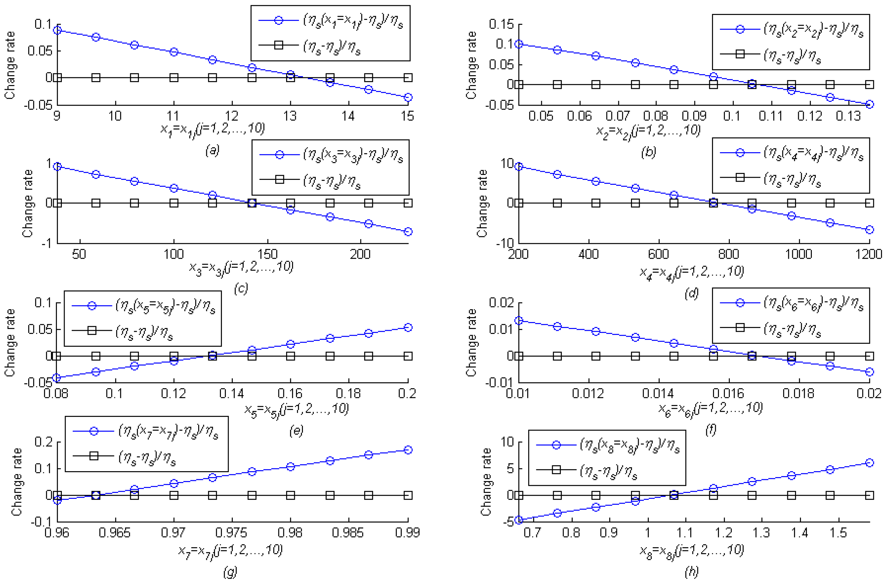
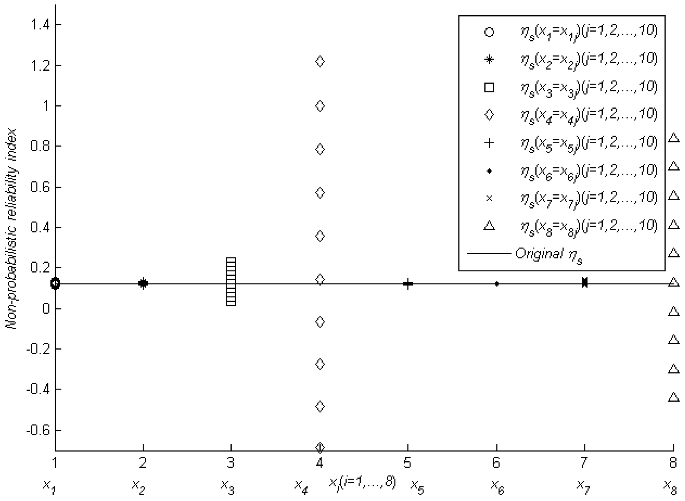
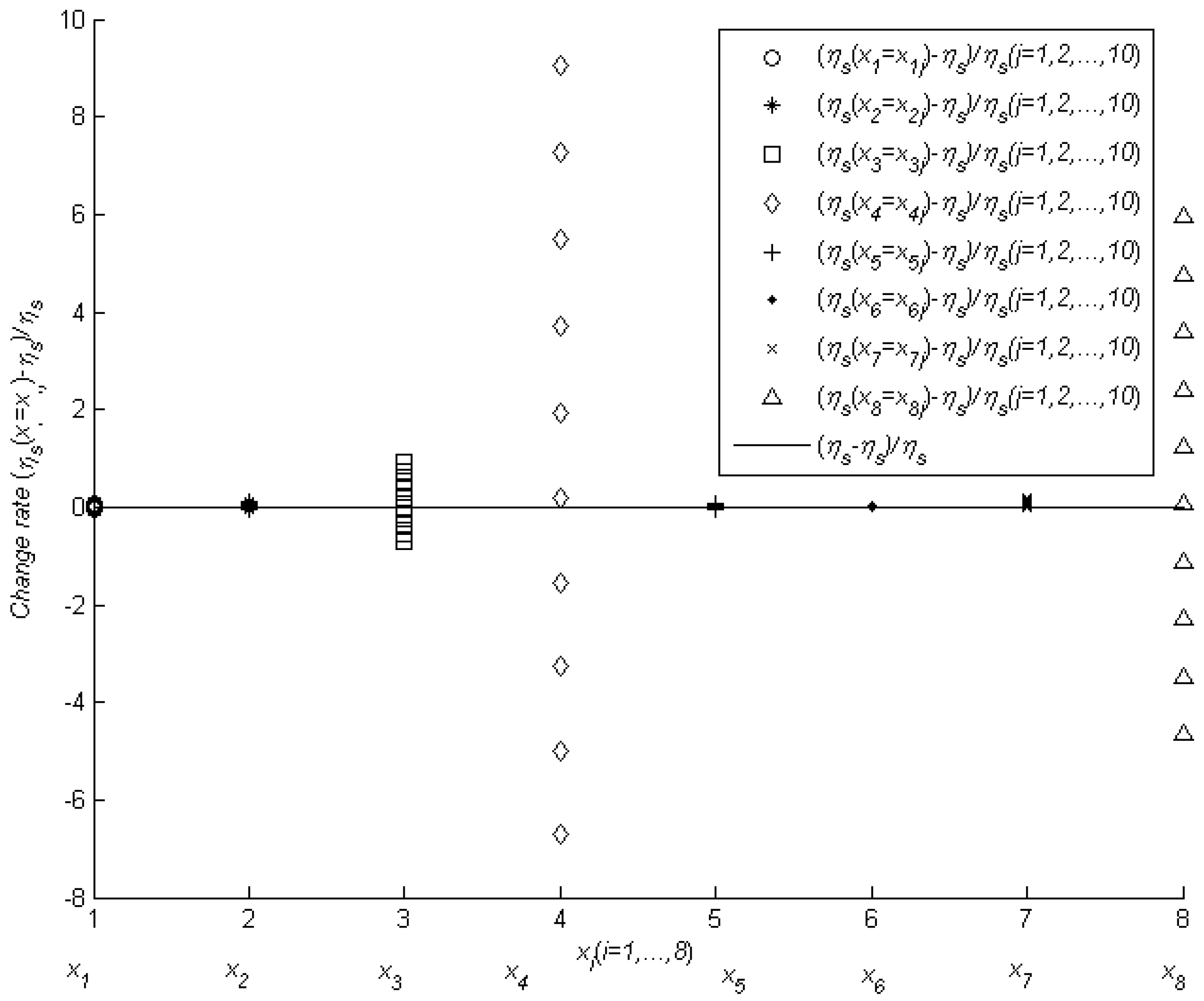
3.2. Evaluation of Sensitivity Analysis for Biodiesel Production with Respect to Interval Parameter

In

Table 2. Results of the proposed sensitivity analysis ${\mathrm{IM}}_i\left(i=1,2,\dots ,8\right)$ and ${\mathrm{IMR}}_i\left(i=1,2,\dots ,8\right)$.

Parameters	${\mathbf{IM}}_{\mathit{i}}\mathbf{\left(}\mathit{i}\mathbf{=}\mathbf{1}\mathbf{,}\mathbf{2}\mathbf{,}\mathbf{\dots }\mathbf{,}\mathbf{8}\mathbf{\right)}$	${\mathbf{IMR}}_{\mathit{i}}\mathbf{\left(}\mathit{i}\mathbf{=}\mathbf{1}\mathbf{,}\mathbf{2}\mathbf{,}\mathbf{\dots }\mathbf{,}\mathbf{8}\mathbf{\right)}$
Capital cost (CC: $x_1$)	4.454 × 10−3	3.680 × 10−2
Interest rate (r: $x_2$)	5.231 × 10−3	4.322 × 10−2
Operating rate (OR: $x_3$)	4.961 × 10−2	4.099 × 10−1
Feedstock price (FP: $x_4$)	4.858 × 10−1	4.013 × 100
Glycerol price (GP: $x_5$)	2.865 × 10−3	2.367 × 10−2
Maintenance rate (MR: $x_6$)	6.643 × 10−4	5.488 × 10−3
Biodiesel conversion efficiency (CE: $x_7$)	9.302 × 10−3	7.685 × 10−2
Biodiesel price (BP: $x_8$)	3.257 × 10−1	2.691 × 100

, we have provided the results of ${\mathrm{IM}}_i$ and ${\mathrm{IMR}}_i$ relevant to $x_i\left(i=1,\dots ,8\right)$. The results show that $x_3$ (operating rate), $x_4$ (price of feedstock), $x_8$ (price of biodiesel), and $x_7$ (biodiesel conversion efficiency) can produce remarkable influences on the economic feasibility of biodiesel production, while the rest of the parameters may generate very lower effects. The importance ranking of the interval parameters can be further gained by the results in Table 2 as: $x_4$ > $x_8$ > $x_3$ > $x_7$ > $x_2$ > $x_1$ > $x_5$ > $x_6$. Compared with the previous results, in which all of the uncertain parameters have been assumed as random variables uniformly distributed within their variation ranges [59], the same importance ranking of sensitivity parameters has been obtained.

The important interval parameters and the non-important ones have been identified by the results in Table 2, specifically: $x_4$, $x_8$, $x_3$, and $x_7$ belong to the important group while $x_2$, $x_1$, $x_5$ and $x_6$ belong to the non-important group. Figure 3 shows the comparison between original NPRI ${\eta }_s$ and conditional NPRI ${\eta }_{s|x_i=x_{ij}}$ with $x_i=x_{ij}$, in which $x_i$ is fixed to a value $x_{ij}$ within its variation interval $\left[{\underset{¯}{x}}_i,{\overline{x}}_i\right]$. Figure 4 shows the change rate between ${\eta }_{s|x_i=x_{ij}}$ and ${\eta }_s$ with respect to ${\eta }_s$, i.e., $\left({\eta }_{s|x_i=x_{ij}}-{\eta }_s\right)/{\eta }_s\left(j=1,2,\dots ,10\right)$, in which $x_i$ is fixed to a value $x_{ij}\in \left[{\underset{¯}{x}}_i,{\overline{x}}_i\right]$, i.e., $x_i=x_{ij}$. Here, $x_{ij}$ takes the following values, i.e., $x_{ij}={\underset{¯}{x}}_i+\left({\overline{x}}_i-{\underset{¯}{x}}_i\right)/\left(10-1\right)\times \left(j-1\right)\left(j=1,2,\dots ,10\right)$. Figure 3 and Figure 4 show that removing the uncertainty related to a non-important parameter $x_i\left(i=1,2,5,6\right)$ and fixing it to any value $x_{ij}\left(i=1,2,5,6\right)$ within its interval $\left[{\underset{¯}{x}}_i,{\overline{x}}_i\right]$ will not exert distinct influence on NPRI ${\eta }_s$, while eliminating the uncertainty associated with an important parameter $x_i\left(i=3,4,7,8\right)$ can cause considerable variation of NPRI ${\eta }_s$.

Figure 5 and Figure 6 have further shown the point figures of ${\eta }_{s|x_i=x_{ij}}$ and $\left({\eta }_{s|x_i=x_{ij}}-{\eta }_s\right)/{\eta }_s$ with $x_{ij}={\underset{¯}{x}}_i+\left({\overline{x}}_i-{\underset{¯}{x}}_i\right)/\left(10-1\right)\times \left(j-1\right)\left(j=1,2,\dots ,10\right)$ for all interval parameters $x_i\left(i=1,2,\dots ,8\right)$. The results shown in Figure 5 and Figure 6 have drawn the same conclusions as Figure 3 and Figure 4.

The previous results show that engineers should focus more concern on these important interval parameters within the project’s lifespan to ensure that biodiesel production is economically feasible. For these non-important interval parameters, taking any value within their ranges will not create remarkable effect on the TEA.

4. Conclusions

This paper employs NPRI to measure the economically feasible extent in the TEA of biodiesel production with uncertainties. Sensitivity analysis of NPRI with regard to uncertain parameters is developed. The final results show that NPRI for biodiesel production is 1.2104 × 10⁻¹ with the interval parameters summarized in Table 1. Price of biodiesel, price of feedstock, and operating cost can cause distinct influence on the economical feasibility of biodiesel production. Compared with our previous study [59], this work has the same decision on TEA and the same importance ranking for uncertain parameters. This method is free of the assumption on distribution, but the previous method is subjected to this assumption in which different assumptions on distribution can result in different results for EIP.

References

1. Höök, M.; Tang, X. Depletion of fossil fuels and anthropogenic climate change—A review. Energy Policy 2013, 52, 797–809. [Google Scholar] [CrossRef]
2. Höök, M. Energy, Climate and Society. 2013. Available online: http://cemusstudent.se/wp-content/uploads/2012/02/Week-49-Energy-Climate-and-Society-Mikael-Höök.pdf (accessed on 3 January 2018).
3. Yan, Y.J.; Li, X.; Wang, G.L.; Gui, X.H.; Li, G.L.; Su, F.; Wang, X.F.; Liu, T. Biotechnological preparation of biodiesel and its high-valued derivatives: A review. Appl. Energy 2014, 113, 1614–1631. [Google Scholar] [CrossRef]
4. Capellán-Pérez, I.; Mediavilla, M.; Castro, C.; Carpintero, O.; Miguel, L.J. Fossil fuel depletion and socio-economic scenarios: An integrated approach. Energy 2014, 77, 641–666. [Google Scholar] [CrossRef]
5. Ellabban, O.; Abu-Rub, H.; Blaabjerg, F. Renewable energy resources: Current status, future prospects and their enabling technology. Renew. Sustain. Energy Rev. 2014, 39, 748–764. [Google Scholar] [CrossRef]
6. Mohr, S.H.; Wang, J.; Ellem, G.; Ward, J.; Giurco, D. Projection of world fossil fuels by country. Fuel 2015, 141, 120–135. [Google Scholar] [CrossRef]
7. Abas, N.; Kalair, A.; Khan, N. Review of fossil fuels and future energy technologies. Futures 2015, 69, 31–49. [Google Scholar] [CrossRef]
8. Nicoletti, G.; Arcuri, N.; Nicoletti, G.; Bruno, R. A technical and environmental comparison between hydrogen and some fossil fuels. Energy Convers. Manag. 2015, 89, 205–213. [Google Scholar] [CrossRef]
9. Day, C.; Day, G. Climate change, fossil fuel prices and depletion: The rationale for a falling export tax. Econ. Model. 2017, 63, 153–160. [Google Scholar] [CrossRef]
10. Mahmudul, H.M.; Hagos, F.Y.; Mamat, R.; Adam, A.A.; Ishak, W.F.W.; Alenezi, R. Production, characterization and performance of biodiesel as an alternative fuel in diesel engines—A review. Renew. Sustain. Energy Rev. 2017, 72, 497–509. [Google Scholar] [CrossRef]
11. No, S.Y. Application of straight vegetable oil from triglyceride based biomass to IC engines—A review. Renew. Sustain. Energy Rev. 2017, 69, 80–97. [Google Scholar] [CrossRef]
12. Othman, M.F.; Adam, A.; Najafi, G.; Mamat, R. Green fuel as alternative fuel for diesel engine: A review. Renew. Sustain. Energy Rev. 2017, 80, 694–709. [Google Scholar] [CrossRef]
13. Efe, S.; Ceviz, M.A.; Temur, H. Comparative engine characteristics of biodiesels from hazelnut, corn, soybean, canola and sunflower oils on DI diesel engine. Renew. Energy 2018, 119, 142–151. [Google Scholar] [CrossRef]
14. Ruhul, A.M.; Kalam, M.A.; Masjuki, H.H.; Shahir, S.A.; Alabdulkarem, A.; Teoh, Y.H.; How, H.G.; Reham, S.S. Evaluating combustion, performance and emission characteristics of Millettia pinnata and Croton megalocarpus biodiesel blends in a diesel engine. Energy 2017, 141, 2362–2376. [Google Scholar] [CrossRef]
15. Silva, M.A.V.D.; Ferreira, B.L.G.; Marques, L.G.D.C.; Murta, A.L.S.; Freitas, M.A.V.D. Comparative study of NOx emissions of biodiesel-diesel blends from soybean, palm and waste frying oils using methyl and ethyl transesterification routes. Fuel 2017, 194, 144–156. [Google Scholar] [CrossRef]
16. Ding, H.; Ye, W.; Wang, Y.Q.; Wang, X.Q.; Li, L.J.; Liu, D.; Gui, J.Z.; Song, C.F.; Ji, N. Process intensification of transesterification for biodiesel production from palm oil: Microwave irradiation on transesterification reaction catalyzed by acidic imidazolium ionic liquids. Energy 2018, 144, 957–967. [Google Scholar] [CrossRef]
17. Zou, C.J.; Zhao, P.W.; Shi, L.H.; Huang, S.B.; Luo, P.Y. Biodiesel fuel production from waste cooking oil by the inclusion complex of heteropoly acid with bridged bis-cyclodextrin. Bioresour. Technol. 2013, 146, 785–788. [Google Scholar] [CrossRef] [PubMed]
18. Ali, C.H.; Qureshi, A.S.; Mbadinga, S.M.; Liu, J.F.; Yang, S.Z.; Mu, B.Z. Biodiesel production from waste cooking oil using onsite produced purified lipase from Pseudomonas aeruginosa FW_SH-1: Central composite design approach. Renew. Energy 2017, 109, 93–100. [Google Scholar] [CrossRef]
19. Tangy, A.; Pulidindi, I.N.; Perkas, N.; Gedanken, A. Continuous flow through a microwave oven for the large-scale production of biodiesel from waste cooking oil. Bioresour. Technol. 2017, 224, 333–341. [Google Scholar] [CrossRef] [PubMed]
20. Allesina, G.; Pedrazzi, S.; Tebianian, S.; Tartarini, P. Biodiesel and electrical power production through vegetable oil extraction and byproducts gasification: Modeling of the system. Bioresour. Technol. 2014, 170, 278–285. [Google Scholar] [CrossRef] [PubMed]
21. Wang, S.X.; Yuan, H.R.; Wang, Y.Z.; Shan, R. Transesterification of vegetable oil on low cost and efficient meat and bone meal biochar catalysts. Energy Convers. Manag. 2017, 150, 214–221. [Google Scholar] [CrossRef]
22. Tang, S.K.; Zhao, H.; Song, Z.Y.; Olubajo, O. Glymes as benign co-solvents for CaO-catalyzed transesterification of soybean oil to biodiesel. Bioresour. Technol. 2013, 139, 107–112. [Google Scholar] [CrossRef] [PubMed]
23. Celante, D.; Schenkel, J.V.D.; Castilhos, F. Biodiesel production from soybean oil and dimethyl carbonate catalyzed by potassium methoxide. Fuel 2018, 212, 101–107. [Google Scholar] [CrossRef]
24. Luna, M.D.G.D.; Cuasay, J.L.; Tolosa, N.C.; Chung, T.W. Transesterification of soybean oil using a novel heterogeneous base catalyst: Synthesis and characterization of Na-pumice catalyst, optimization of transesterification conditions, studies on reaction kinetics and catalyst reusability. Fuel 2017, 209, 246–253. [Google Scholar] [CrossRef]
25. Li, K.; Fan, Y.L.; Zeng, L.P.; Han, X.T.; Yan, Y.J. Burkholderia cepacia lipase immobilized on heterofunctional magnetic nanoparticles and its application in biodiesel synthesis. Sci. Rep. 2017, 7, 16473. [Google Scholar] [CrossRef] [PubMed]
26. Nisar, J.; Razaq, R.; Farooq, M.; Iqbal, M.; Khan, R.A.; Sayed, M.; Shah, A.; Rahman, I. Enhanced biodiesel production from Jatropha oil using calcined waste animal bones as catalyst. Renew. Energy 2017, 101, 111–119. [Google Scholar] [CrossRef]
27. Quinn, J.C.; Davis, R. The potentials and challenges of algae based biofuels: A review of the techno-economic, life cycle, and resource assessment modeling. Bioresour. Technol. 2015, 184, 444–452. [Google Scholar] [CrossRef] [PubMed]
28. Rodríguez, R.P.; Borroto, Y.S.; Espinosa, E.A.M.; Verhelst, S. Assessment of diesel engine performance when fueled with biodiesel from algae and microalgae: An overview. Renew. Sustain. Energy Rev. 2017, 69, 833–842. [Google Scholar] [CrossRef]
29. Taparia, T.; Mvss, M.; Mehrotra, R.; Shukla, P.; Mehrotra, S. Developments and challenges in biodiesel production from microalgae: A review. Biotechnol. Appl. Biochem. 2015, 63, 715–726. [Google Scholar] [CrossRef] [PubMed]
30. Piligaev, A.V.; Sorokina, K.N.; Samoylova, Y.V.; Parmon, V.N. Lipid production by microalga Micractinium sp. IC-76 in a flat panel photobioreactor and its transesterification with cross-linked enzyme aggregates of Burkholderia cepacia lipase. Energy Convers. Manag. 2018, 156, 1–9. [Google Scholar] [CrossRef]
31. Probst, K.V.; Schulte, L.R.; Durrent, T.P.; Rezac, M.E.; Vadlani, P.V. Oleaginous yeast: A value-added platform for renewable oils. Crit. Rev. Biotechnol. 2016, 36, 942–955. [Google Scholar] [CrossRef] [PubMed]
32. Sitepu, I.R.; Garay, L.A.; Sestric, R.; Levin, D.; Block, D.E.; German, J.B.; Mills, K.L.B. Oleaginous yeasts for biodiesel: Current and future trends in biology and production. Biotechnol. Adv. 2014, 32, 1336–1360. [Google Scholar] [CrossRef] [PubMed]
33. Zhang, K.; Pei, Z.J.; Wang, D.H. Organic solvent pretreatment of lignocellulosic biomass for biofuels and biochemicals: A review. Bioresour. Technol. 2016, 199, 21–33. [Google Scholar] [CrossRef] [PubMed]
34. Lam, S.S.; Mahari, W.A.W.; Jusoh, A.; Chong, C.T.; Lee, C.L.; Chase, H.A. Pyrolysis using microwave absorbents as reaction bed: An improved approach to transform used frying oil into biofuel product with desirable properties. J. Clean. Prod. 2017, 147, 263–272. [Google Scholar] [CrossRef]
35. Malhotra, R.; Ali, A. Lithium-doped ceria supported SBA−15 as mesoporous solid reusable and heterogeneous catalyst for biodiesel production via simultaneous esterification and transesterification of waste cottonseed oil. Renew. Energy 2018, 119, 32–44. [Google Scholar] [CrossRef]
36. Abdullah, S.H.Y.S.; Hanapi, N.H.M.; Azid, A.; Umar, R.; Juahir, H.; Khatoon, H.; Endut, A. A review of biomass-derived heterogeneous catalyst for a sustainable biodiesel production. Renew. Sustain. Energy Rev. 2017, 70, 1040–1051. [Google Scholar] [CrossRef]
37. Singh, V.; Sharma, Y.C. Low cost guinea fowl bone derived recyclable heterogeneous catalyst for microwave assisted transesterification of Annona squamosa L. seed oil. Energy Convers. Manag. 2017, 138, 627–637. [Google Scholar] [CrossRef]
38. Vinod, B.M.; Madhu, M.K.; Amba, P.R.G. Butanol and pentanol: The promising biofuels for CI engines—A review. Renew. Sustain. Energy Rev. 2017, 78, 1068–1088. [Google Scholar]
39. Singh, L.K.; Chaudhary, G. Advances in Biofeedstocks and Biofuels; John Wiley & Sons: Hoboken, NJ, USA, 2017. [Google Scholar]
40. Sotoft, L.F.; Rong, B.G.; Christensen, K.V.; Norddahl, B. Process simulation and economical evaluation of enzymatic biodiesel production plant. Bioresour. Technol. 2010, 101, 5266–5274. [Google Scholar] [CrossRef] [PubMed]
41. Haas, M.J.; McAloon, A.J.; Yee, W.C.; Foglia, T.A. A process model to estimate biodiesel production costs. Bioresour. Technol. 2006, 97, 671–678. [Google Scholar] [CrossRef] [PubMed]
42. Ong, H.C.; Mahlia, T.M.I.; Masjuki, H.H.; Honnery, D. Life cycle cost and sensitivity analysis of palm biodiesel production. Fuel 2012, 98, 131–139. [Google Scholar] [CrossRef]
43. Xin, C.H.; Addy, M.M.; Zhao, J.Y.; Cheng, Y.L.; Cheng, S.B.; Mu, D.Y.; Liu, Y.H. Comprehensive techno-economic analysis of wastewater-based algal biofuel production: A case study. Bioresour. Technol. 2016, 211, 584–593. [Google Scholar] [CrossRef] [PubMed]
44. Kern, J.D.; Hise, A.M.; Characklis, G.W.; Gerlach, R.; Viamajala, S.; Gardner, R.D. Using life cycle assessment and techno-economic analysis in a real options framework to inform the design of algal biofuel production facilities. Bioresour. Technol. 2017, 225, 418–428. [Google Scholar] [CrossRef] [PubMed]
45. Thomassen, G.; Dael, M.V.; Lemmens, B.; Passel, S.V. A review of the sustainability of algal-based biorefineries: Towards an integrated assessment framework. Renew. Sustain. Energy Rev. 2017, 68, 876–887. [Google Scholar] [CrossRef]
46. Dutta, S.; Neto, F.; Coelho, M.C. Microalgae biofuels: A comparative study on techno-economic analysis & life-cycle assessment. Algal Res. 2016, 20, 44–52. [Google Scholar]
47. Hpffman, J.; Pate, R.C.; Drennen, T.; Quinn, J.C. Techno-economic assessment of open microalgae production systems. Algal Res. 2017, 23, 51–57. [Google Scholar] [CrossRef]
48. Xin, C.H.; Addy, M.M.; Zhao, J.Y.; Cheng, Y.L.; Ma, Y.W.; Liu, S.Y.; Mu, D.Y.; Liu, Y.H.; Chen, P.; Ruan, R. Waste-to-biofuel integrated system and its comprehensive techno-economic assessment in wastewater treatment plants. Bioresour. Technol. 2018, 250, 523–531. [Google Scholar] [CrossRef] [PubMed]
49. Mandegari, M.A.; Farzad, S.; Görgens, J.F. Recent trends on techno-economic assessment (TEA) of sugarcane biorefineries. Biofuel Res. J. 2017, 4, 704–712. [Google Scholar] [CrossRef]
50. Tao, L.; Milbrandt, A.; Zhang, Y.N.; Wang, W.C. Techno-economic and resource analysis of hydroprocessed renewable jet fuel. Biotechnol. Biofuels 2017, 10, 261. [Google Scholar] [CrossRef] [PubMed]
51. Patel, M.; Zhang, X.L.; Kumar, A. Techno-economic and life cycle assessment on lignocellulosic biomass thermochemical conversion technologies: A review. Renew. Sustain. Energy Rev. 2015, 53, 1486–1499. [Google Scholar] [CrossRef]
52. Busse, S.; Brümmer, B.; Ihle, R. Price formation in the German biodiesel supply chain: A Markov-switching vector error-correction modeling approach. Agric. Econ. 2012, 43, 545–560. [Google Scholar] [CrossRef]
53. Mankiw, N.G. Principles of Economics, 6th ed.; South-Western Cengage Learning: Mason, OH, USA, 2011. [Google Scholar]
54. Borgonovo, E.; Peccati, L. Uncertainty and Global Sensitivity Analysis in the Evaluation of Investment Projects. Int. J. Prod. 2006, 104, 62–73. [Google Scholar] [CrossRef]
55. Brownbridge, G.; Azadi, P.; Smallbone, A.; Bhave, A.; Taylor, B.; Kraft, M. The future viability of algae-derived biodiesel under economic and technical uncertainties. Bioresour. Technol. 2014, 151, 166–173. [Google Scholar] [CrossRef] [PubMed]
56. López, P.P.; Montazeri, M.; Feijoo, G.; Moreira, M.T.; Eckelman, M.J. Integrating uncertainties to the combined environmental and economic assessment of algal biorefineries: A Monte Carlo approach. Sci. Total Environ. 2018, 626, 762–775. [Google Scholar] [CrossRef] [PubMed]
57. Abubakar, U.; Sriramula, S.; Renton, N.C. Stochastic techno-economic considertations in biodiesel production. Sustain. Energy Technol. Assess. 2015, 9, 1–11. [Google Scholar]
58. Tang, Z.C.; Lu, Z.Z.; Liu, Z.W.; Xiao, N.C. Uncertainty analysis and global sensitivity analysis of techno-economic assessments for biodiesel production. Bioresour. Technol. 2015, 175, 502–508. [Google Scholar] [CrossRef] [PubMed]
59. Xia, Y.J.; Tang, Z.C. A novel perspective for techno-economic assessments and effects of parameters on techno-economic assessments for biodiesel production under economic and technical uncertainties. RSC Adv. 2017, 7, 9402–9411. [Google Scholar] [CrossRef]
60. Sajid, Z.; Zhang, Y.; Khan, F. Process design and probabilistic economic risk analysis of biodiesel production. Sustain. Prod. Consum. 2016, 5, 1–15. [Google Scholar] [CrossRef]
61. Liew, W.H.; Hassim, M.H.; Ng, D.K.S. Sustainability assessment framework for chemical production pathway: Uncertainty analysis. J. Environ. Chem. Eng. 2016, 4, 4878–4889. [Google Scholar] [CrossRef]
62. Batan, L.Y.; Graff, G.D.; Bradley, T.H. Techno-economic and Monte Carlo probabilistic analysis of microalgae biofuel production system. Bioresour. Technol. 2016, 219, 45–52. [Google Scholar] [CrossRef] [PubMed]
63. Ochoa, M.P.; Estrada, V.; Maggio, J.D.; Hoch, P.M. Dynamic global sensitivity analysis in bioreactor networks for bioethanol production. Bioresour. Technol. 2016, 200, 666–679. [Google Scholar] [CrossRef] [PubMed]
64. Yao, G.L.; Staples, M.D.; Malina, R.; Tyner, W.E. Stochastic techno-economic analysis of alcohol-to-jet fuel production. Biotechnol. Biofuels 2017, 10, 18. [Google Scholar] [CrossRef] [PubMed]
65. Garay, A.G.; Miquel, M.G.; Gosalbez, G.G. High-Value Propylene Glycol from Low-Value Biodiesel Glycerol: A Techno-Economic and Environmental Assessment under Uncertainty. ACS Sustain. Chem. Eng. 2017, 5, 5723–5732. [Google Scholar] [CrossRef]
66. Trading Economics. Malaysia Interest Rate 1996–2014. 2014. Available online: http://zh.tradingeconomics.com/malaysia/bank-lending-rate (accessed on 3 January 2018).
67. Hitchcock, G. The Economics of Biofuel Production and Use. 2014. Available online: http://www.sts-technology.com/docs/Economics-of-biofuel-production-and-use.ppt (accessed on 3 January 2018).
68. Duncan, J. Costs of Biodiesel Production. 2003. Available online: http://www.globalbioenergy.org/uploads/media/0305_Duncan_-_Cost-of-biodiesel-production.pdf (accessed on 3 January 2018).
69. Nagi, J.; Ahmed, S.K.; Nagi, F. Palm Biodiesel an Alternative Green Renewable Energy for the Energy Demands of the Future. In Proceedings of the International Conference on Construction and Building Technology, Kuala Lumpur, Malaysia, 16–20 June 2008; pp. 79–94. [Google Scholar]
70. Nanda, M.R.; Yuan, Z.; Qin, W.; Poirier, M.A.; Chunbao, X. Purification of Crude Glycerol using Acidification: Effects of Acid Types and Product Characterization. Austin J. Chem. Eng. 2014, 1, 1–7. [Google Scholar]
71. FarmdocDAILY. Recent Trends in Biodiesel Prices and Production Profits. 2013. Available online: http://farmdocdaily.illinois.edu/2013/09/recent-trends-in-biodiesel.html (accessed on 3 January 2018).
72. Cremona, C.; Gao, Y. The possibilistic reliability theory: Theoretical aspects and applications. Struct. Saf. 1997, 19, 173–201. [Google Scholar] [CrossRef]
73. Guo, S.X.; Lu, Z.Z.; Feng, Y.S. A non-probabilistic model of structural reliability based on interval analysis. Chin. J. Comput. Mech. 2001, 18, 56–60. [Google Scholar]
74. Guo, S.X.; Li, Y. Non-probabilistic reliability method and reliability-based optimal LQR design for vibration control of structures with uncertain-but-bounded parameters. Acta Mech. Sin. 2013, 29, 864–874. [Google Scholar] [CrossRef]
75. Kang, Z.; Luo, Y. Non-probabilistic reliability-based topology optimization ofgeometrically nonlinear structures using convex models. Comput. Methods Appl. Mech. Eng. 2009, 198, 3228–3238. [Google Scholar] [CrossRef]
76. Ben-Haim, Y.; Elishakoff, I. Convex Models of Uncertainty in Applied Mechanics; Elsevier Press: Amsterdam, The Netherlands, 1990. [Google Scholar]
77. Ben-Haim, Y. A non-probabilistic measure of reliability of linear systems based on expansion of convex models. Struct. Saf. 1995, 17, 91–109. [Google Scholar] [CrossRef]
78. Ben-Haim, Y. Robust Reliability in the Mechanics Sciences; Springer: Berlin, Germany, 1996. [Google Scholar]
79. Ben-Haim, Y. Robust reliability of structures. Adv. Appl. Mech. 1997, 33, 1–41. [Google Scholar]
80. Elishakoff, I. Essay on uncertainties in elastic and viscoelastic structures: From A. M. Freudenthal’s criticisms to modern convex modeling. Comput. Struct. 1995, 56, 871–895. [Google Scholar] [CrossRef]
81. Elishakoff, I. Are Probabilistic and Anti-Optimization Approaches Compatible? Whys and Hows in Uncertainty Modelling: Probability, Fuzziness and Antioptimization; Springer: New York, NY, USA, 1999. [Google Scholar]
Figure 1. Diagrammatic presentation for non-probabilistic reliability index (NPRI) of a system with two intervals, (a) normalized limit state function (LSF) intersects with enlarged square box at one side; (b) normalized limit state curve (LSC) intersects with enlarged square box at another side; and (c) normalized limit state curve intersects with enlarged square box at cater-corner point.
Energies 11 00588 g001
Figure 2. Variation ranges of total profit (TotalProfit: USD), net present value (NPV: USD), and y j = g j ( x ) due to economic and technical uncertainties.
Energies 11 00588 g002
Figure 3. Original NPRI η s and conditional NPRI η s | x i = x i j ( j = 1 , 2 , , 10 ) , in which x i is fixed to a value x i j [ x ¯ i , x ¯ i ] , i.e., x i = x i j ( j = 1 , 2 , , 10 ) .
Energies 11 00588 g003
Figure 4. Change rate between η s | x i = x i j and η s with respect to η s , i.e., ( η s | x i = x i j η s ) / η s ( j = 1 , 2 , , 10 ) , in which x i is fixed to a value x i j [ x ¯ i , x ¯ i ] , i.e., x i = x i j .
Energies 11 00588 g004
Figure 5. Point figure for conditional NPRI η s | x i = x i j with x i = x i j ( i = 1 , 2 , , 8 ; j = 1 , 2 , , 10 ) .
Energies 11 00588 g005
Figure 6. Point figure for change rate between η s | x i = x i j and η s with respect to η s , ( η s | x i = x i j η 0 ) / η 0 with x i = x i j ( i = 1 , 2 , , 8 ; j = 1 , 2 , , 10 ) .
Energies 11 00588 g006