A Domestic Microgrid with Optimized Home Energy Management System
by
 , , , , and
Zafar Iqbal
1 ,
,
Nadeem Javaid
2,* ,
,
Saleem Iqbal
1,
Sheraz Aslam
2, 
Zahoor Ali Khan
3,
Wadood Abdul
4,
Ahmad Almogren
4 and
Atif Alamri
4 1
PMAS Arid Agriculture University, Rawalpindi 4600, Pakistan
2
COMSATS Institute of Information Technology, Islamabad 44000, Pakistan
3
CIS, Higher Colleges of Technology, Fujairah 4114, UAE
4
Research Chair of Pervasive and Mobile Computing College of Computer and Information Sciences, King Saud University, Riyadh 11633, Saudi Arabia
*
Author to whom correspondence should be addressed.
Energies 2018, 11(4), 1002; https://doi.org/10.3390/en11041002
Submission received: 28 February 2018
/
Revised: 10 April 2018
/
Accepted: 13 April 2018
/
Published: 20 April 2018
(This article belongs to the Special Issue Building Energy Use: Modeling and Analysis)
Abstract
:Microgrid is a community-based power generation and distribution system that interconnects smart homes with renewable energy sources (RESs). Microgrid efficiently and economically generates power for electricity consumers and operates in both islanded and grid-connected modes. In this study, we proposed optimization schemes for reducing electricity cost and minimizing peak to average ratio (PAR) with maximum user comfort (UC) in a smart home. We considered a grid-connected microgrid for electricity generation which consists of wind turbine and photovoltaic (PV) panel. First, the problem was mathematically formulated through multiple knapsack problem (MKP) then solved by existing heuristic techniques: grey wolf optimization (GWO), binary particle swarm optimization (BPSO), genetic algorithm (GA) and wind-driven optimization (WDO). Furthermore, we also proposed three hybrid schemes for electric cost and PAR reduction: (1) hybrid of GA and WDO named WDGA; (2) hybrid of WDO and GWO named WDGWO; and (3) WBPSO, which is the hybrid of BPSO and WDO. In addition, a battery bank system (BBS) was also integrated to make our proposed schemes more cost-efficient and reliable, and to ensure stable grid operation. Finally, simulations were performed to verify our proposed schemes. Results show that our proposed scheme efficiently minimizes the electricity cost and PAR. Moreover, our proposed techniques, WDGA, WDGWO and WBPSO, outperform the existing heuristic techniques.
1. Introduction
Recently, increasing energy consumption has been observed around the globe. Presently, most power is produced from fossil fuels that increase carbon emissions. To minimize carbon emissions and fulfill the inevitably increasing electricity demand, scientists have explored the alternative sources of energy generation, i.e., renewable energy sources (RESs). Moreover, complexity of power system is significantly increased due to the penetration of RESs. However, the large-scale installation of RESs to the existing conventional power system will increase the vulnerability of already heavily loaded power system [1]. For this purpose, the transform of the current electric power system to the smart grid, i.e., the unification of advanced information and communication technologies (ICTs) with conventional power grid, is one of the best solutions [2]. These technologies not only exploit the stability and reliability of the power system but also enable the smart grid to efficiently incorporate the RESs and DG.
RESs have gained prominence over traditional and fossil fuel-based energy sources, which also contribute to environmental degradation. Therefore, policy makers and researchers are being compelled to think about changing the form of energy generation. The DG emerges with the emergence of RESs [3]. A microgrid is considered as a lower layer of the smart grid, and is an independent small scale power generation system that supplies power to the electricity consumers [4]. Microgrid operates in three different modes: grid-connected mode, where it is needed to sell power back or purchase to/from main grid; off-grid mode, where power is not available from the utility grid; and isolated mode, where utility grid is in far and remote areas.
Numerous articles have been published about isolated microgrid.The authors discussed stand-alone microgrid consisting of photovoltaic (PV) source, wind turbine and storage that are mathematically formulated to design voltage regulation policy and control-based load tracking system. They proposed a control and energy management policy. According to this strategy, the storage can be charged by constant current and voltage which increases its lifespan. It was also considered in this study that the power demand is less than the generated power [5].
The burgeoning population continuously increases the use of electric appliances which results in increasing power demand. To fulfill this increasing demand of electricity, RESs become lucrative for scientists because the conventional sources of electricity generation are costly and cause high carbon emissions. Hence, it is necessary to generate more power locally from RESs. In addition, we have to optimize the existing power sources to create alternative methods of power generation. To achieve this end, researchers are working on the utilization of renewable energy generation in power sector to make it more efficient. A smart grid is a simple conventional electric grid with the use of ICTs integrated, while microgrid is part of a smart grid. According to the concept of a microgrid, the power could be used in a reliable and optimized way and more energy will be locally generated. The power of a microgrid will fulfill the energy requirement along with the considerable reduction in cost and peak-to-average ratio (PAR).
In smart grid, the common goals of different demand response (DR) and demand side management (DSM) strategies are the reduction in electricity bill and PAR. Load shifting schemes are used to achieve balance energy consumption. To design an effective home energy management system (HEMS), different algorithms are used by research community, e.g. mixed integer linear programming (MILP) [6], dynamic programming (DP), multi parametric programming (MPP) [7], integer linear programming (ILP) [8], etc. However, these algorithms have unpredictable energy consumption patterns and cannot handle a large range of different home appliances. Furthermore, authors in [9,10,11,12,13,14] focused on electricity cost reduction and PAR minimization through stochastic, mathematical and heuristics techniques.
The work presented in [9,10,11,12,13,14] either focused on specific area (cost reduction, PAR minimization, etc.) or failed to gain full benefit from the smart grid technologies to present efficient HEMS. The motivation for this work was to reduce the deficiencies of existing HEMSs. This work introduced an optimized HEMS. The proposed HEMS minimized the consumer’s electricity cost and PAR with maximum user comfort (UC) while integrating battery bank system (BBS) and RESs simultaneously in the residential sector. Moreover, the RTP tariff was used for electricity cost calculation and we implemented four heuristic techniques, grey wolf optimization (GWO), binary particle swarm optimization (BPSO), genetic algorithm (GA), and wind-driven optimization (WDO), to achieve aforesaid objectives. We also proposed three hybrid optimization algorithms: wind-driven GA (WDGA), wind-driven GWO (WDGWO) and wind-driven BPSO (WBPSO). Part of this work was already published in [15]. The main contributions of this work are as follows:
- We proposed three hybrid schemes: WDGA, WDGWO and WBPSO.
- This work considered the grid-connected microgrid system with multiple appliances.
- Our proposed work minimized the electricity cost and PAR.
- By implementing our proposed schemes, user can enjoy maximum comfort.
- Imported electricity was also reduced by integrating microgrid.
The reminder of the paper is organized as follows: literature review is provided in Section 2. Motivation and problem statement is discussed in Section 3. Section 4 explains the mathematical formulation of the problem using a mathematical technique called MKP. Energy generation using PV, wind and BBS charging and discharging are discussed in Section 4.1, Section 4.2 and Section 4.3, while Section 4.4, Section 4.5, Section 4.6, Section 4.7 and Section 4.8 discuss the energy consumption, energy pricing and electricity cost, PAR, appliances waiting time (AWT) and objective function, respectively. Section 5 presents the proposed system model, while the optimization techniques, GWO, GA, BPSO, WDO, WDGA, WDGWO and WBPSO, are described in Section 6. In Section 7 simulation results and discussion are provided. Section 8 presents conclusion and future work.
2. Literature Review
In the literature, significant amount of work has been done in smart grid, microgrid, macrogrid and hybrid energy generation to optimize energy consumption, energy consumption cost and PAR. Researchers are further working to introduce alternative methods for local energy generation that are less expensive, easy to generate and environment friendly. Some research work indicated that the combination of RESs into residential sector provides the most cost effective solutions. This hybridization of RESs and use of distributed energy resources (DERs) make energy more flexible, reliable, and sustainable and removes redundancies. Some related work has been cited below and a summary of the cited work is presented in Table 1.
The authors proposed a residential microgrid consisting of RESs in [9]. To obtain an efficient and realistic management, the domestic load was divided into three different types. They introduced the anxiety range concepts for consumers behavior. The designed model generates a schedule for all components of the microgrid when operating day-ahead and results show daily cost saving of 10%. The authors discussed the time-of-use (TOU) based energy management system along with ESS integration in [10]. The economic and technical evaluation is carried out using different battery technologies. Their experimental results show that the integration of ESS with TOU significantly reduce the cost.
In [11], a controller strategy was proposed that acts as a controller between grid and PV or wind generators with battery storage system. The connection device provided the ancillary services. In this paper, the authors proposed a three-steps control strategy. The methodology managed the collaboration between RESs and DERs, keeping in view the use of domestic energy. The main objectives of this study were: user comfort, peak shaving and forming virtual power plants [12].
This work proposed a new decision support and management system (DSEMS) keeping in view the residential load consumption [13]. The designed system acts as finite state machine (FSM). The FSM consists of different scenarios based on consumers preferences. The work in [14] discussed an intelligent home energy management algorithm. The algorithm manages the power consumption of domestic appliances with DR analysis. The household load is managed using priority and the total domestic load is constrained below a certain threshold level. The work provide an insight for performing DR activities for residential consumers. In the next section, the motivation and problem is explained in detail.
Marc Beaudin et al. provided a comprehensive review of HEMS in [16]. HEMS is an efficient tool for shifting and reducing the energy production and consumption of a residential area. HEMS plays an important role for demand response. By considering multiple objectives, i.e., user comfort, energy costs, load profile and environmental concerns, HEMS creates an optimal energy consumption schedule for home appliances. A stochastic programming model (SPM) was presented in [17]. The authors considered the environmental and economic aspects using RESs. Using Monte Carlo method and roulette wheel mechanism the uncertain parameters are modeled for 24 h duration considering demand and supply. The authors formulated the optimization problem as a stochastic multi-objective linear programming problem.
In [18], the authors presented an efficient HEMS for DSM in residential area. They used the combination of two pricing schemes for cost calculation: time of use (ToU) and real-time price. To minimize peak creation, GA is used in this work. Simulation results show that the combination of TOU and RTP is favourable for cost and PAR reduction. However, there exists a trade-off between the UC and electricity cost.
The authors in [19] described the scheduling of home appliances. Their objectives was to optimize electricity consumption pattern. For appliances and the RESs scheduling, MILP was investigated. They generated electricity locally from RESs and it reduced the electricity cost and the excess energy generated is sold back to the commercial grid to further minimize the electricity cost. Although RESs combined with HEMS is useful for both the consumers and the utility, the installation cost of RESs is expensive for a single home or consumer.
The authors of [20] proposed an optimal energy management model for a grid-connected solar power and battery hybrid system is discussed. Their model optimizes the electricity cost while keeping in view constraints such as power balance, solar output and battery capacity limits. They used the open and closed loop method to dispatch the power flow in real-time based on uncertain distributions. These two methods led to great cost saving and robust control performance. Furthermore, the authors did not consider UC.
A power scheduling problem with RESs and energy storage was investigated in [21]. They prioritized the appliances into five classes and proposed a novel formulation and solution for this model using mixed integer programming (MIP). MIP made the problem more complex and could not handle many appliances. They also ignored the UC.
In [22], authors proposed an autonomous hybrid power system (HPS), they used supervisory control and data acquisition (SCADA) for this purpose. In autonomous HPS, they integrated diesel generation with wind and solar power, which increases the availability of power. Solar generates DC electricity which is converted to AC via inverter. However, they did not consider minimization of AWT for maximum UC.
The authors in [23] proposed a framework for the HEMS modeling and techno-economical sizing using MILP. The sizing of additional DG and BBS are discussed for smart home appliances. They investigated the DR activities for daily energy consumption demand profile as compared to normal daily energy consumption profile of household appliances. They focused on decreasing cost, varying load and distributed generation profile for different seasons for DG and BBS. They also considered different sensitivity analysis keeping in view the impact of variations of economic input for the provided model for a long-term analysis. However, the authors did not consider minimization of AWT for UC maximization. The authors in [24] discussed the comparison of GA and particle swarm optimization (PSO) for computational complexity. Their results illustrate that PSO have lesser computational complexity to attain a desired result as compared to GA.
In [25], authors presented an operational planning model of microgrid considering multiple DR programs. They defined two objective functions, cost and emission, which have been optimized using epsilon constraint multi-objective optimization. The authors used MILP and did not consider PAR and optimization of UC.
Authors presented and designed a distributed energy management strategy (DEMS) for the optimal operation of microgrid. They considered the problem as an optimal power flow problem [26]. In this model, the microgrid central controller and the local controller compute an optimal schedule. They applied the proposed distributed energy management system (EMS) to a real microgrid consisting of solar, wind turbines, diesel generators and a BBS. They tested the distributed EMS in both islanded and grid-connected mode and showed that their proposed algorithm converges quickly. The authors did not consider UC optimization.
In [27], authors proposed a hybrid energy microgrid model and discussed energy scheduling problem. Their model consisted of solar, wind power, combined heat energy storage system and electric vehicle (EV). The objective function was cost optimization, which includes operational, gas, electric power, storage and EV charging–discharging cost reduction. They proposed a multi-team PSO (MTPSO) and units, groups and swarm information are used to update velocity. MTPSO has stable conversion as compared to PSO. However, the authors did not consider UC.
In [28], the improved version of PSO (IPSO) was used for optimization. The goal of IPSO is to minimize cost. Results illustrate that the user load curve and the objective curve nearly become the same by the proposed IPSO. On the other hand, electricity price and the objective curve have an inverse relationship. Power system stability was one of the objective functions, and the proposed scheme rejected the load in peak hours and thus the UC was compromised. In [29], the authors introduced the concept of peer-to-peer energy sharing by those who can afford renewable and non-renewable electricity generation sources such as solar panel, generator and a windmill to those who cannot afford such sources of renewable energy generation or lack access to main grid. This would create a marketplace for electricity and self-sufficiency in power market. To this end, an ad hoc microgrid was introduced using a power management unit (PMU). However, the authors did not reduce PAR. Sheraz et al. proposed a cost-efficient scheme using cuckoo search and GA in [30]. Their proposed scheme efficiently minimized the electricity cost but UC is not taken into account. A MILP based HEM scheme was proposed in [31] for electric cost and imported load reduction from external grid. They integrated microgrid which consists of wind turbine and solar panel with electrical vehicle (mobile storage). Simulation results show that their proposed scheme reduces the total cost and imported load.
3. Motivation and Problem Description
With the rapid growth in population, the electricity demand in residential area is also increasing. The residential sector consumes almost 40% of the electricity [32]. To meet the energy demand, various methods of power generation have been explored. The existing and outdated power systems cannot meet the current power demand required by consumers. It is too old and cannot withstand the pressure of peak power demand. Increased population has rendered the whole power transmission and distribution system incapacitated, fragile and worn out. In addition, the existing old power system is often subjected to power interruptions due to cumbersome maintenance procedures.
The authors designed a HEMS model considering ToU pricing scheme and RES integration in [33]. Their model uses evolutionary algorithms, i.e., cuckoo search, BPSO and GA, to optimally consume RESs and grid energy. The proposed HEMS model significantly reduced high peaks and electricity cost. Furthermore, the simulation results show that cuckoo search shows supremacy as compared to other counter parts. However, they did not consider minimization of AWT for enhancing UC.
In [34], the authors studied the sizing of the storage units and the scheduling of RESs in microgrid. They considered the uncertain nature of the microgrid and associated load. The authors made a hybrid of chaos optimization algorithm and BPSO, i.e., chaos BPSO (CBPSO), which shows enhanced global search capability compared to BPSO. Their results show that CBPSO reduces the electricity cost and microgrid network losses efficiently. However, the authors did not consider peak reduction and UC maximization.
The authors in [35] provided study of domestic load scheduling problem. To satisfy the budget of the consumers, the authors proposed a load scheduling algorithm. They considered ToU pricing scheme to manage the total energy consumption . Mixed integer nonlinear programming (MINLP) was used for problem formulation. However, this problem was difficult to solve and had high computational complexity. To reduce the computational complexity and solve the problem easily, they introduced the generalized bender decomposition approach. They solved the optimization problem providing optimal load scheduling of appliances having different operation characteristics and energy consumption pattern. However, by scheduling the appliances and satisfying the budget limit, the UC was compromised.
Many techniques such as MILP [36], DP [37], convex programming (CP) [38], linear programming (LP) [39], ILP [40] and bacterial foraging algorithm (BFA) [41] are used to design an efficient HEMS. However, in some cases, these techniques cannot handle many appliances and their convergence rate is also very slow. Moreover, with these techniques, the maximization of UC, use of dynamic pricing schemes and integration of RESs with the system are almost ignored. Therefore, in this work, we used GWO [42], GA [42], BPSO [43], WDO [44] and the proposed hybrid techniques, i.e., WDGA, WDGWO and WBPSO, to design an efficient HEMS in term of low cost, energy consumption pattern, and minimum PAR with maximum UC.
4. Formulation of the Problem Statement
In this section, we have mathematically formulated our problem by defining an objective function along with few constraints. The detailed description of the formulation is presented as follows.
4.1. PV Generation
The smart home we proposed is equipped with a rooftop PV generation system, as solar energy is less costly than other RESs (biomass, wind, biogas, tidal and geothermal) and available everywhere. The Earth receives a huge amount of solar radiation and most of the areas with population have insulation levels of 150–300 watts/m [45]. The output power from a PV panel is given in Equation (1) [46,47,48].
where total electricity generated by PV is presented by , G shows solar irradiation (W/m), is solar radiation at reference conditions = 1000 W/m), the cell temperature at reference conditions is C), is the temperature coefficient (in this work, a value of C) is adopted) and depicts the cell temperature which is calculated by the Equation (2), [48].
where represents the ambient temperature.
4.2. Wind Generation
Wind is a very promising source of renewable energy. USA, China, Germany, Spain, Denmark and India are the leading countries in power generation from wind using wind turbine. Power from the wind can be given by the following Equation (3), [49,50].
where shows the rotor swept (blade) area of wind turbine in m, the air density is represented by in kg/m, the average wind velocity is shown by V in m/s and is a power coefficient which shows the efficiency of a wind turbine (maximum value of 0.59). The output power available from wind turbine depends on wind speed and can be given by Equation (4) taken from [51].
where , and are the rated, cut-out and cut-in wind speeds, respectively. The rated output power of wind turbine is shown by . Wind turbine power output and wind speed is given in Figure 1 [52].
4.3. BBS
The capacity of the BBS is calculated by Equation (5) in time slot t [54].
where DOD shows the allowable depth of discharge, is daily energy consumption, AD is a number of autonomy days, and and are the voltage and BBS efficiency, respectively. Energy charging and discharging by the BBS during the time period from t-1 to t can be given by Equation (6) [55].
where and show the available power (which may consumed by consumer) in BBS at time slot t and (t-1), respectively. The symbol denotes the self-discharge rate of the BBS and it is assumed as 0.002 in our study. is the power from battery bank in time slot t. The value of remains between and during charging operation of the BBS, as given by Equation (7).
where and are minimum and maximum allowable energy levels in the BBS. Furthermore, the BBS is charged from own microgrid and commercial grid when electricity prices are low, and charged electricity is used in high price hours.
4.4. Energy Consumption
We assume that t represents a single time slot and T represents total time horizon, which is 24 h. Set of appliances in home is denoted by S and each appliance is denoted by and consumes an amount of energy in time slot t such that t ∈ T.
The daily energy consumption by non-deferrable load (NDL), interruptible load (IL) and must-run load (MRL) and the total energy consumed in whole day by all appliances are calculated in Equations (8)–(11), respectively [56].
where , and are the energy consumption of NDl, IL and MRL appliances, respectively, denoted by . is the total energy consumption of NDL, IL and MRL appliances.
4.5. Energy Pricing and Electricity Cost
Many pricing schemes in existence are defined per unit energy cost. Some of the pricing schemes are RTP, peak pricing (PP), critical peak pricing (CPP), TOU pricing, real-time market pricing (RTMP), non-critical peak (NCP), locational marginal pricing (LMP), hourly pricing (HP), and critical peak pricing with rebate (CPP-R) [57,58]. However, most of the work on appliances scheduling consists of the DAP or TOU pricing scheme. In TOU scheme, the time is divided into multiple time slots. In this work, we use RTP scheme, which remains constant for one time slot and varies from one slot to another slot. The electricity cost against each class (NDL, IL and MRL) of appliances and total electricity cost of all appliances are calculated by Equations (12)–(15), respectively.
where is RTP signal in time slot t. , and are the ON/OFF state of NDL, IL and MRL appliances as shown in Equation (16)–(18), respectively. , and are the electricity prices of NDL, IL and MRL appliances in time slot t, respectively. ps show the price signal, while , , , , , and represent NDL, IL and MRL appliances and SN, SI and SM represent the set of appliances of NDL, IL and MRL, respectively.
4.6. PAR
PAR balancing is necessary to bring equilibrium of demand and supply between consumers and utility. The PAR is very important for cost savings, achieving stable system and increasing spinning reserve system capacity. The PAR also helps in reducing peak load demand, peak power plants cost, transmission line losses, increasing of electrical equipment life, etc. Let the peak and average load of the smart home be denoted by and , respectively. Then, the PAR of the demanded load can be given in Equation (19) [59].
4.7. AWT
Let denote the AWT of all smart appliances. is an AWT term which introduces the start time, stop time, maximum waiting time, length of operation time (LOT), and minimum waiting time of appliances such that . Now, the AWT can be given by Equation (20) [60].
where is appliance waiting time, is the appliance ON time, is the appliance start time, is the appliance LOT and is the appliance maximum waiting time.
The AWT is 0 if start time and on time are equal, i.e., . On the other hand, if the earliest starting time of any appliance and ON time (when any appliance starts execution) is different, i.e., , then consumer has to wait to perform the operation of the appliance.
4.8. Objective Function
The reduction in electricity cost, PAR and AWT for maximum UC were the basic objectives of this study which are achieved by proper management of smart appliances. PAR reduction is important for both utility and consumers to minimize the operation time of peak power plants and backup generators. We supposed that there is single smart home (electricity consumer) in a residential area with HEMS and is consuming electricity from commercial grid and owned microgrid. Furthermore, our proposed schemes did not affect any liberalized electricity market. We formulated the optimization problem using MKP. From a set of appliances, we selected an appliance for a particular hour to be ON or OFF. Each appliance has a single unique weight and value, which shows the ON/OFF state and power rating, respectively. To allow any smart appliance to perform its operation in particular time slot, EMC decides based on defined objective function (Equation (21)). The constraints must be satisfied by the total weight i.e., the total energy consumed by appliances is explained in Equation (21) and the constraints in Equations (22)–(24).
Objective function:
Subject to:
where , and are the energy consumption of NDL, IL and MRL appliances in time slot t, respectively. , and are the available energy from PV, wind and battery in time slot t, respectively. is the total energy consumption caused by all smart appliances in particular time slot t. is the available energy from utility grid that a consumer can import in time slot t. is the minimum amount of energy consumed in unscheduled case. and are the lower and upper limit of scheduling horizon, respectively. shows the scheduling time of appliances. In Equation (23), constraint is defined to bring balance between the energy of demand and supply.
5. System Model
In proposed system model, each electricity consumer has a HEMS. The smart user uses RESs, BBS, and energy from the electric grid for meeting their load requirements. Here, the RESs consists of PV and wind turbine and Table 2 shows the assumed rating of the system model components. The appliances are scheduled to minimize electricity expenses, PAR and maximum UC. Furthermore, the appliances are categorized into three classes by consumers, i.e., NDLAs, which cannot be shifted to another time slot; NDLAs have start and end points to describe its time-span and we assumed that consumer cannot compromise in these type of appliances; and ILA, the load of particular consumers that, according to the agreement, can be cut off by the supply undertaking for a limited period. Its operation can be suspended in the middle. The interruptible appliance has a task having various sequences of operation which can be interrupted. MRLA must be run immediately at any time. These appliances are not shiftable, non-deferrable and non-interruptible. They must be run at any cost, as presented in Table 3. Furthermore, all appliances considered in this work are connected to an alternating current (AC) system.
The proposed system model is shown in Figure 2 and consists of smart meter (SM), energy management controller (EMC), smart scheduler unit (SMSU), advanced metering infrastructure (AMI), PV and wind power generation system, solar charge controller, DC/AC inverters, appliances and BBS.
Bi-directional communication between consumers and utility is only possible by integrating AMI, and works as a backbone for the smart grid. The responsibility of AMI includes the hourly load demand and the electricity rates between utility and SM. Utility and smart home communicate with each other via SM, which acts as a communication gateway between them. The processing, reading, and sending of energy consumption data and receiving of pricing signals are the main function of an SM. RESs are the real alternative sources of local power generation to fossil fuel. RESs mainly consist of PV system, fuel cells, hydro and wind turbines, while, in our case, they consist of PV and wind turbine. PV panel generates electricity which is DC and then converted to AC via converter. A BBS works as a both sink and source of energy and is considered as a suitable solution for RES integration in the residential sector. Therefore, in the proposed system model, BBS power is used to exploit the PV and wind system energy efficiently and to alleviate the electricity cost and PAR. An SMSU is programmed using heuristic algorithms and works in between the SM and EMC. The optimal energy consumption pattern for all appliances is generated by SMSU and then it sends the scheduling pattern to the EMC for further processing. EMC control the BBS and operation of all appliances according to the generated scheduled by SMSU. EMC is the core of the proposed system model.
6. Optimization Techniques
The objective function for optimization of appliances scheduling discussed in Section 4.8 was solved using nature-inspired algorithms such as GWO, WDGWO, GA, BPSO, WDO, WDGA and WBPSO. Therefore, we adopted heuristic technique to solve our optimization problem. Furthermore, heuristic algorithms provide alternative ways for solving complex problems and have better performance as compared to other techniques.
6.1. GWO
GWO algorithm represents the hunting mechanism and leadership hierarchy of grey wolves which is proposed in [61]. To understand the leadership hierarchy, there are four types of wolves, i.e., alpha, beta, delta and omega. To perform optimization, four main steps are implemented in GWO, i.e., hunting, searching, encircling and attacking prey. Grey wolves always live in a pack with average size of 12–15. Encircling prey can be mathematically given in Equation (25) and (26) below.
where and are coefficient vectors, t represents the current iteration, the position vector of the prey is represented by , and the position vector of a grey wolf is shown by . To update the position of the search agents, Equations (27)–(33) are used.
With the help of these equations, a search agent updates its position in n-dimensional search space. The position is updated according to alpha, beta and delta. The parameters used for GWO are given in Table 4.
6.2. GA
GA belongs to heuristic optimization family and is inspired from the genes of living organisms. GA works on the basis of iteration and having different possible iterations with different possible solutions [62]. The structure of GA consists of binary coded chromosomes which are randomly initialized. The ON/OFF state of the appliances is represented by the binary coded chromosomes pattern of GA and length of chromosomes show the total number of smart appliances represented in Equation (34).
With the creation of initial population, the fitness function of GA is evaluated as the objective function of this study. The new population is generated by implementing mutation and crossover operators. The parameters used in this work are presented in Table 5.
A whole new generation will be produced if crossover probability is 100%, while the new generation produced will be an exact copy of the parents if the probability of crossover is 0%. However, pre-mature convergence to the suboptimal solution is avoided by larger crossover rate for optimization problems, which is why 90% is the best crossover rate, as given in Equation (35) below.
The mutation process is used for randomness creation in the results. One or more genes are mutated in a chromosome from its original state. The probability of mutation is given below:
After crossover and mutation process, the generated population and its fitness are compared with the previous individuals.
6.3. BPSO
BPSO is a discrete variant of PSO and consists of four main steps, i.e., particle’s initial position and initial velocity, and local and global best positions among the particles. The PSO randomly generates and disperses population in the search space. BPSO updates velocity and position by following Equations (37) and (38), respectively [63,64].
where , , , and are the position and velocity of particle i in the d dimension at time slots t and t-1, respectively. and are the best positions obtained by particle i and swarm in d dimension in time slot t and t-1, respectively. and are the two acceleration coefficients. and are random numbers between 0 and 1. The sigmoid function for position is given below.
where shows the velocity of the particle. The parameters of BPSO are explained in Table 6.
6.4. WDO
WDO is a heuristic optimization algorithm. Instead of particles in BPSO, it works on the basis of atmospheric motion of air parcels. WDO is differentiated from the other heuristic techniques due to the existence of forces. Friction force resists the motion of air parcels in forward direction. Gravitational force is a vertical force. Coriolis force deflects the air parcels in the atmosphere. Pressure gradient moves the parcels in the forward direction. These forces can be mathematically represented in Equations (39)–(42) [44].
where and show Coriolis force and earth rotation, respectively. is wind velocity, is gravitational force, is air density, is air finite volume, g is acceleration of gravity, pressure gradient force is presented by , shows pressure gradient, is friction force and is friction coefficient.
Equations (43) and (44) [44] represent the air parcel’s position and velocity.
and
where and represent the current and new velocity of the air parcels, respectively. and show the current and new positions of the air parcels, respectively. is the global best position. R, T, , g and c are universal gas constant, temperature, the coefficient of friction, gravity and Coriolis force, respectively. r is a variable value for the rank of air parcels.
Random solutions are created by WDO and then a new population is generated by updating the velocities and evaluating the fitness function. To attain an optimal appliances pattern, the fitness function of updated and previous generation of air parcels are compared. The term pressure in WDO is fitness function, i.e., in GA, PSO and BPSO. The parameters of WDO are described in Table 7.
6.5. WDGA
WDGA is the hybrid of GA and WDO. In WDGA, first, steps of the WDO are performed, i.e., initialization of population and selection. Then, instead of using velocity updating step of WDO, crossover and mutation operators from GA are performed for the generation of new population to ensure diversity in the solution. The reason for replacing velocity step of WDO with crossover and mutation operators of GA is the increase in time complexity which degrades the performance of WDO when the input value is large. Thus, in our work, WDGA generated random solutions in the form of 0 and 1 (0 and 1 show the appliance status OFF and ON, respectively). After initialization of population, these solutions were evaluated according to our defined objective function (minimum electricity cost and PAR) in Equation (21). The proposed WDGA algorithm is given in Algorithm 1 and its parameters are given in Table 8.
6.6. WDGWO
WDGWO is an optimization technique that is developed by GWO and WDO algorithms. The WDGWO works initially the same as GWO, however, the position of the search agents of the GWO is replaced by iterative velocity updating parameter of the WDO. In WDO, velocity updating step is better for new generation as compared to GWO updating method. This hybrid version of GWO and WDO gives better results than GWO and WDO, separately. In our work, the initial population (in the form of 0 and 1) was generated on the basis of wolves, i.e., alpha, beta, delta and omega. The selection was also performed according to our objective function by GWO and velocity updating is performed to regenerate best population. In every iteration, our proposed WDGWO found local best solutions and finally it found the global best on the basis of local solutions. The pseudocode of the WDGWO is shown in Algorithm 2. Table 9 shows the parameters that are used for simulations in WDGWO.
6.7. WBPSO
In this section, we discuss WBPSO algorithm which merges WDO and BPSO. The WBPSO algorithm is more efficient in solving optimization problems as compared to WDO and BPSO because WBPSO consists of the best properties of both aforementioned algorithms. The pseudocode of this hybrid algorithm is shown in Algorithm 3. The WBPSO works similarly to BPSO, i.e., random population generation, finding the local and global best positions of particles by changing velocity, and updating position of the particles in each iteration. When the stopping criteria are fulfilled, the algorithm stops working and generates random solutions that are different from the previous results. In our work, population generation step was performed by BPSO in binary form (0 and 1 show OFF and ON status of each appliance, respectively). After population generation, best solutions were selected on the basis of our defined objective function in Equation (21). WDO wind pressure was used for new solution generation. Finally, the global best solutions (for each hour) were selected having minimum electricity cost and PAR. The parameters of WBPSO are given in Table 10.
| Algorithm 1 WDGA | |
| Input: set of appliances or population; | |
| Initialization genetic parameters: peak hour, off peak hour, t = 0, H, vmax, vmin, no of iteration; Initialization wind driven parameters: dimMin, dimMax, dim, param.rt, param.g, param.alp, param.c; | |
| 1: | fordo |
| 2: | for do |
| 3: | Generate population randomly; |
| 4: | for do |
| 5: | Fitness calculation; Select best population, pop save in pop1; Status check of appliance using peak hour and off peak hour; |
| 6: | if t == peak hour then |
| 7: | Shift on RESs and BBS; |
| 8: | OR wait for off peak hour; |
| 9: | if Consumption == high then |
| 10: | Check remaining t of all App and check LOT until it is 0; |
| 11: | end if |
| 12: | end if |
| 13: | end for |
| 14: | Generate new population; |
| 15: | Replace the genetic operators by particles pressure; |
| 16: | Evaluate and find air parcels (population) pressure; |
| 17: | for do |
| 18: | for do |
| 19: | x(K,h) = (dimMax - dimMin) * ((x(K,h)+1)./2) + dimMin; |
| 20: | Pres(K,h) = sum ; |
| 21: | end for |
| 22: | end for |
| 23: | Save air parcels value in pop2; |
| 24: | Check and find air parcels velocity; |
| 25: | Vel = min(vel, maxV); and vel = max(vel, -maxV); |
| 26: | Find and update air parcel positions; |
| 27: | x = x + vel; and x = min(x, 1.0); and x = max (x, -1.0); |
| 28: | Finding best particle in population |
| 29: | Globalpres, indx = min (pres); and globalx = x (indx, :); |
| 30: | Find min location for this iteration |
| 31: | Minpres, indx = min (pres); and minpos = x (indx, :); |
| 32: | Rank the air parcels: sortedpres rankind = sort (pres); |
| 33: | Sort the air parcels position, velocity and pressure: |
| 34: | Pres = sortedpres; |
| 35: | Updating the global best: |
| 36: | Better = minpres < globalpres; |
| 37: | if Solution = better then |
| 38: | Globalpres = minpres; |
| 39: | Globalpos = minpos; |
| 40: | end if |
| 41: | Save the velocity and position value in pop3; |
| 42: | Select from pop2 and pop3; |
| 43: | New velocity and position of air parcels; |
| 44: | if Solution == infeasible then |
| 45: | Update solution; |
| 46: | Update with sol in pop2 and pop3; |
| 47: | end if |
| 48: | Update pop best solution; |
| 49: | Update t = t+1 till 24 h; |
| 50: | Terminate when t = 24 h or iter = Max; |
| 51: | end for |
| 52: | end for |
| Algorithm 2 WDGWO | |
| Input: set of appliances or population; | |
| Initialization grey wolf parameters: Max iter, Np, D, alpha, beta, delta, search agents; | |
| Initialization wind driven parameters: dimMin, dimMax, dim, param.rt, param.g, param.alp, param.c; | |
| 1: | Randomly initialize the position of search agents i.e., positions = rand (Np, D); |
| 2: | Evaluate the position of search agents |
| 3: | whiledo |
| 4: | for do |
| 5: | Calculate objective function for each search agent Fitness = sum (electricity cost * positionsx); Update alpha, beta and delta |
| 6: | if then |
| 7: | |
| 8: | |
| 9: | end if |
| 10: | if then |
| 11: | |
| 12: | |
| 13: | end if |
| 14: | if then |
| 15: | |
| 16: | |
| 17: | end if |
| 18: | end for |
| 19: | ; a value linearly from 2 to 0 |
| 20: | for do |
| 21: | for do |
| 22: | r1, r2 randomly initialize the value between 0 to 1 |
| 23: | Vel = maxV * 2 * (rand (Np, D)-0.5) |
| 24: | for do |
| 25: | for do |
| 26: | Velot (i, j) = vel (i, j); |
| 27: | Vel (i, j) = ( 1 - alp ) * vel (i, j) - ( g * positions (i, j)) + abs (1 - 1/i) * (((positions (i, j) - positions (i, j))).* RT ) + ( c * velot (i, j) / i) |
| 28: | if ((vel (i, j) < vmax) and (vel (i, j) > vmin)) then |
| 29: | Velot (i, j) = vel (i, j); |
| 30: | else if ( vel (i, j) < vmin ) then |
| 31: | Vel (i, j) = vmin |
| 32: | else if (vel (i, j) > vmax) then |
| 33: | Vel (i, j) = vmax; |
| 34: | end if |
| 35: | Position updating |
| 36: | Sig (i, j) = 1/(1+exp (-vel (i, j))); |
| 37: | if rand (1) < sig (i, j) then |
| 38: | Positions (i, j) = 1; |
| 39: | else |
| 40: | Positions (i, j) = 0; |
| 41: | end if |
| 42: | end for |
| 43: | end for |
| 44: | end for |
| 45: | end for |
| 46: | end while |
| Algorithm 3 WBPSO | |
| Require: Number of particles, swarm size, , electricity price, LOT and appliance power consumption rating | |
| Require: vmax, vmin, no of iter, c1, c2, param.RT, param.g, param.alp, param.c, dimMin, dimMax, dim | |
| 1: | Randomly generate the particles’ positions and velocities |
| 2: | |
| 3: | fortodo |
| 4: | Initialize (swarmsize, tbits) |
| 5: | |
| 6: | |
| 7: | |
| 8: | end for |
| 9: | for h = 1 to 24 do |
| 10: | Validate constraints |
| 11: | for to M do |
| 12: | if then |
| 13: | |
| 14: | end if |
| 15: | if then |
| 16: | |
| 17: | else |
| 18: | |
| 19: | end if |
| 20: | Decrement one from the TOT of the working appliance |
| 21: | if > then |
| 22: | if then |
| 23: | Switch the load to RESs and BBS |
| 24: | else |
| 25: | Consume the grid energy |
| 26: | end if |
| 27: | end if |
| 28: | Return |
| 29: | Vel = maxV * 2 * (rand (swarm, n)-0.5); |
| 30: | for i = 1 : swarm do |
| 31: | for j = 1 : n do |
| 32: | Velot (i, j) = vel (i, j); |
| 33: | Vel (i, j) = ( 1 - param.alp ) * vel (i, j) - ( param.g * pres (i, j)) + abs (1 - 1/i) * (((pres (i, j) - pres (i, j))).*param.RT) + (param.c * velot (i, j) /i); |
| 34: | if ((vel (i, j) < = vmax) and (vel (i, j) >= vmin)) then |
| 35: | vel (i, j) = vel (i, j); |
| 36: | elseif ( vel (i, j) < vmin); vel (i, j) = vmin; elseif ( vel (i, j) > vmax); vel (i, j) = vmax; |
| 37: | end if |
| 38: | Sig (i, j) = 1 / ( 1 + exp ( -vel (i, j))); |
| 39: | if rand (1) < sig (i, j) then |
| 40: | x (i, j) = 1; |
| 41: | else |
| 42: | x (i, j) = 0; |
| 43: | end if |
| 44: | end for |
| 45: | end for |
| 46: | Check velocity: vel = min (vel, maxV); vel = max (vel, -maxV); |
| 47: | Update air parcel positions: x = x + vel; x = min (x, 1.0); x = max (x, -1.0); |
| 48: | Evaluate population: (pressure) |
| 49: | Finding best particle in population |
| 50: | Globalpres, indx = min (pres); globalx = x (indx, :); |
| 51: | Min location for this iteration |
| 52: | Minpres, indx = min (pres); minpos = x (indx, :); |
| 53: | Rank the air parcels; |
| 54: | Sorted-pres rank-ind = sort (pres); |
| 55: | Sort the air parcels position, velocity and pressure; |
| 56: | Pres = sorted-pres; |
| 57: | Updating the global best; |
| 58: | Better = minpres < globalpres; |
| 59: | if Better then |
| 60: | Globalpres = minpres; globalpos = minpos; |
| 61: | end if |
| 62: | end for |
| 63: | end for |
7. Simulation Results and Discussion
This section shows the detailed results of the simulations that we performed in MATLAB to validate our proposed schemes. In our work, we uncovered the effect of microgrid integration and effect of temperature and wind speed on the electricity generation from PV panel and wind turbine, respectively. The heuristic algorithms GA, GWO, BPSO, and WDO as well as proposed WDGA, WDGWO and WBPSO were used to evaluate the performance of our proposed scheme in terms of electricity cost, PAR and AWT with and without RES integration.
7.1. RTP Scheme
Figure 3 explains the RTP signal in each time slot. The price signal is given in cents/kWh. In time slot 1, the price is 10 cents/kWh and during 2.5–4.5 the price is 10.4 cents/kWh. During time slot 8, the price is highest, i.e., above 25 cents/kWh. During time slots 10–16, the price is reduced and remains 20–10 cents/kWh. During time slots 14–24, the price signal is stable and remains below 10 cents/kWh.
7.2. Energy Consumption Profile
Total energy consumption of all appliances is discussed in this section. The energy consumption behavior can be described by defining some arbitrary thresholds. The thresholds of the load defined are 15 kW is a high peak, 12–14 kW is peak load, 5–8 kW is moderate load, 3–5 kW is minimum load and 1–2 kW is the negligible load. The hourly energy consumption with and without RES integration is shown in Table 11. Approximately 66% of the energy is use from grid and 34% from RESs. Table 12 shows cost for each hour randomly taken with and without RES integration. After the integration of RESs, the hourly difference and percentage cost reduction with and without RES integration is depicted in Table 12. Table 13 shows similar statistics but for total daily cost.
7.2.1. Energy Consumption with and without RESs
Figure 4, Figure 5 and Figure 6 show the energy consumption profile of the consumers without and with RES integration. The energy consumption pattern can be seen in Figure 4 by heuristic algorithms, in the case of unscheduled, GA, WDO, and WDGA and after the integration of RESs. In Figure 5, the energy consumption pattern is shown for unscheduled, GWO, WDO and WDGWO and the integration of RESs. Figure 6 shows the energy consumption pattern by unscheduled, BPSO, WDO and WBPSO. Figure 4 shows the energy consumption pattern via GA, WDO and their hybrid version, i.e., WDGA. It can be seen in Figure 4 that, after integrating RESs, the consumption pattern changes in each hour. During time slots 6–13, the unscheduled load is high and reaches 15 KW. The peak load by GA during time slots 4–6 can be seen in both subplots in Figure 4: without RES integration it is 14 KW and with RES integration it is below 10 KW. Similarly, the peak load by WDO during time slots 1, 11 and 15 is equal to or slightly above 14 KW, while after RES integration it is significantly below 14 KW. The energy consumption pattern of WDGA and WDGA-RESs can also be compared in both subplots.
Figure 5 represents the energy consumption with GWO, WDO and their hybrid, i.e., WDGWO. The unscheduled load is similar in both subplots, while the load by GWO and GWO-RESs can be seen in both subplots, which show a significant reduction after the integration of RESs. The reduction by WDO can also be observed in both subplots in Figure 5. The pattern of energy consumption by WDGWO and WDGWO-RESs is also shown in both subplots. Figure 6 represents the energy consumption pattern of appliances by unscheduled, BPSO, WDO and their hybrid, i.e., WBPSO. The unscheduled load is the same in both cases, while the energy consumption pattern by BPSO can be seen in both subplots. The peak load is equal to 8 KW in the case of without RES integration and below 6 KW in the case of RES integration. The energy consumption by WDO can also be seen in both cases, which show significant load optimization. The consumption patterns by WBPSO and WBPSO-RESs can be seen in Figure 6. All the hybrid versions of the proposed algorithms, i.e., WDGA, WDGWO and WBPSO, are perform better than their parent techniques.
7.3. Electricity Cost
The total hourly electricity cost by proposed algorithms WDGA, WDGWO and WBPSO are shown in Figure 7, Figure 8 and Figure 9 without and with RES integration, respectively. While Figure 10 shows the total cost of one day without and with RES integration, Table 12 and Table 13 show the hourly and total one day cost with and without RES integration.
Electricity Cost Profile with and without RESs
The electricity cost profile shown in Figure 7 explains the unscheduled cost, and cost after scheduling the load by GA, WDO and their hybrid WDGA. The unscheduled cost is the highest during time slots 8–10 and lowest for time slots 15–24. The cost of GA during time slots 9–10 and 13–15 is high, while during time slots 2–3, 6–7, 16–18 and 20–24 is low, i.e., below 50 cents. The cost of WDO is highest during time slots 8-10, while lowest for 16–24. The cost is reduced by GA-RESs, WDO-RESs and WDGA-RESs and its curve are very smooth, as shown in Figure 7. The cost is below 100 cents for 24 h. The cost of WDGA shown in Figure 7 is much less than its parent algorithms. The cost is highest for time slots 14–15, i.e., 100 cents, and lowest for time slots 11–14, i.e., 45 cents.
Figure 8 shows the electricity cost profile by WDGWO and WDGWO-RESs. The unscheduled cost during time slot 7–13 is high both with RES and without RES integration. The cost for GWO, WDO, and WDGWO before and after integration of RESs, i.e., GWO-RESs, WDO-RESs and WDGWO-RESs, can be compared in Figure 8. The cost for WDGWO is between 0 and 200 cents, while the cost for WDGWO-RESs is between 0 and 100 cents.
The cost for WBPSO is shown in Figure 9. The cost for BPSO and BPSO-RESs can also be seen in the figure. The cost of WDO and WDO-RESs is also represented in Figure 9, which shows much reduction in cost when RES is integrated. While the cost of WBPSO and WBPSO-RESs shows similar behavior, the cost of WBPSO and WBPSO-RESs is much more than BPSO and WDO. The total costs for one day using WDGA, WDGWO, WBPSO, WDGA-RESs, WDGWO-RESs, and WBPSO-RESs are shown in Figure 10. The unscheduled cost is same in all subplots, while WDGWO, WDGA, WBPSO, WDGWO-RESs, WDGA-RESs and WBPSO-RESs reduce the cost more than their parent] algorithms because of their hybrid features. Table 13 shows the cost statistics with and without RES integration.
7.4. PAR
The performance of the proposed algorithms WDGWO, WDGA and WBPSO evaluated in terms of PAR is discussed in this section and shown in Figure 11. It is evident in Figure 11 that PAR is reduced significantly in the case of scheduling by these algorithms as compared to the unscheduled electricity consumption.
PAR with and without RESs
The PAR is shown without the integration of RES in Figure 11. The PAR is very high in unscheduled case, while, in the case of scheduling the load using GWO, WDO, WDGA, GA, BPSO, WDGA and WBPSO, the PAR is low as compared to the unscheduled scenario. The PAR using WDGA is less than WDO and GA but more than BPSO, as BPSO has reduced the PAR much more compared to all other algorithms. The PAR using WDGWO is less than WDO and GWO. After the integration of RESs and BBS, the major portion of the load is shifted to RESs and a small portion of load remains on the grid. Therefore, the PAR is further reduced as shown in Figure 11. The PAR in the unscheduled case is very high, while, in the case of GA-RESs, GWO-RESs, WDO-RESs, and BPSO-RESs, it is very low as compared to the case in which RESs is not integrated. The PAR with the proposed algorithms, i.e., WDGA, WDGWO, and WBPSO, is further reduced as compared to the GA-RESs, GWO-RESs, WDO-RESs and BPSO-RESs. Table 14 shows the reduction in PAR with and without RES integration.
7.5. AWT
Figure 12 shows the AWT of appliances by scheduling the appliances with the proposed algorithms, i.e., WDGA, WDGWO and WBPSO. The AWT using GWO, GA and BPSO is almost three hours, while the AWT using WDO is almost two hours less than GWO and the AWT using the proposed algorithms are further reduced and less than both GWO and WDO. This shows the performance of the proposed algorithms is better than their parent algorithms.
7.6. Energy Generation Profile of Microgrid
In this section, the power generation from microgrid is discussed. The microgrid consists of PV and wind power generation as discussed below.
7.6.1. Energy Generation with Wind Turbine and Solar Panel
The energy generation from wind turbine is depicted in Figure 13. The energy generation from wind turbine is based on the wind speed presented in Figure 14. If the wind speed is high, maximum energy will be generated; otherwise, if the wind speed is low, less energy will be generated. During time slots 11–20, the wind speed is high, i.e., above 10 and 15 m/s, and the energy generation is also high, i.e., 1.5–3.5 kWh. The energy generation is below 0.5 kW during time slots 1–6 and 21–24 because the wind speed is very slow in these time slots, as shown in Figure 14. Figure 14 shows that the wind speed is the highest during time slot 12 so the energy generation is also highest, i.e., above 3 kWh. The relationship between wind generation and wind speed is shown in Table 15.
The hourly electricity generation by PV panel is shown in Figure 13. As the PV generation depends on solar radiation and external temperature, it only generates energy during the daytime. The PV generates energy during time slots 5–18, i.e., only 13 h out of 24 h on average, as shown in Figure 14. The maximum or peak generation is only 4–5 h depending on sunlight, temperature, panel tilt angle and geographical location. As can be seen in Figure 14, the temperature of the day is high during time slots 5–18 so the generation is also high. During time slots 1–4 and 19–24, the temperature is below 20 C and there is no solar Irradiation , therefore the PV generation is zero. Table 15 shows the effect of temperature on PV generation.
8. Conclusion and Future Work
The monitoring and control of daily power consumption may help to prevent energy wastage and minimize electricity cost and PAR. In this work, HEM schemeswere proposed to minimize electricity cost and PAR with maximum UC in residential area. We also integrated wind turbine and PV panel for cheaper electricity generation to reduce electricity cost. To achieve the above-mentioned objectives, we implemented existing heuristics techniques: GA, BPSO, WDO and GWO. Moreover, we proposed three hybrid techniques: WDGA, WDGWO, and WBPSO. A comparison between our proposed and the existing schemes is also presented and our hybrid schemes outperformed in terms of electricity cost and PAR reduction. It is clearly observed from simulation results that our proposed schemes achieve the defined objectives. After the integration of microgrid, the electricity cost is reduced by 35.02%, 35.60% and 53.39% using WDGA, WDGWO and WBPSO, respectively. The PAR is minimized using WDGA, WDGWO and WBPSO by 61.30%, 61.43% and 18.89%, respectively.
In the future, the same classes of appliances will be considered; however, a hybrid renewable energy generation system including PV, diesel generator, battery bank and wind turbines will be designed. Plug-in hybrid electric vehicle (PHEV) and battery electric vehicle (BEV) will be considered in a remote grid. To optimize energy cost and satisfy the budget limit, techno-economic analysis of the hybrid system will also be carried out.
Acknowledgments
This project was full financially supported by the King Saud University, through the Vice Deanship of Research Chairs.
Author Contributions
All authors have equal contribution.
Conflicts of Interest
The authors declare no conflict of interest.
Abbreviations
The following abbreviations are used in this manuscript:
| Acronyms | Description |
| Alternate current | |
| Autonomy days | |
| Advanced Information Networking and Applications | |
| Advanced metering infrastructure | |
| Appliances waiting time | |
| Battery bank storage | |
| Battery electric vehicle | |
| Bacterial foraging algorithm | |
| Binary particle swarm optimization | |
| Chaos BPSO | |
| Convex programming | |
| Critical peak pricing | |
| Critical peak price with rebate | |
| Day-ahead pricing | |
| Direct current | |
| Distributed energy management strategy | |
| Distributed energy resources | |
| Distributed generation | |
| Depth of discharge | |
| Dynamic programming | |
| Demand response | |
| Demand side management | |
| Energy consumption | |
| Energy consumption and generation | |
| Energy management controller | |
| Energy management system | |
| Electricity price | |
| Energy storage system | |
| Electric vehicle | |
| Genetic algorithm | |
| Grey wolf optimization | |
| Hourly pricing | |
| Hybrid power system | |
| Home energy management system | |
| Information and communication technologies | |
| Interruptible load | |
| Interruptible load appliances | |
| Integer linear programming | |
| Improved PSO | |
| Kilowatt | |
| Kilowatt hour | |
| Locational marginal pricing | |
| Length of operation time | |
| Linear programming | |
| Mixed integer programming | |
| Mixed-integer linear programming | |
| Mixed integer nonlinear programming | |
| Multiple knapsack problem | |
| Model predictive control | |
| Multi-parametric programming | |
| Must-run load | |
| MRLA | Must run load appliances |
| Multi-team PSO | |
| Non-critical peak | |
| Non-deferrable load | |
| Non-deferrable load appliances | |
| Optimal control method | |
| Peak-to-average ratio | |
| Plug-in electric vehicle | |
| Personal computer | |
| Predictor corrector proximal multiplier | |
| Plug-in hybrid electric vehicle | |
| Phaser measurement unit | |
| Power management unit | |
| Peak pricing | |
| Price signal | |
| Particle swarm optimization | |
| Photovoltaic | |
| Autonomy days | |
| Hourly pricing | |
| Price signal | |
| Renewable energy | |
| Renewable energy sources | |
| Real-time market pricing | |
| RTP | Real time pricing |
| SCADA | Supervisory control and data acquisition |
| SI | Set of IL appliances |
| SM | Smart meter |
| SM | Set of must-run appliances |
| SMSU | Smart schedular unit |
| SN | Set of NDL appliances |
| T | Temperature |
| TOU | Time of use |
| UC | User comfort |
| USA | United States of America |
| WBPSO | Wind driven BPSO |
| WDGA | Wind driven genetic algorithm |
| WDGWO | Wind driven GWO algorithm |
| WDO | Wind driven optimization |
| Symbol | Description |
| PV panel output power | |
| Solar radiation at reference conditions | |
| Temperature coefficient of the PV panel | |
| Air density | |
| Wind turbine power coefficient | |
| S | Set of appliances |
| Cut-in wind speed | |
| BBS storage capacity | |
| BBS voltage | |
| Available power from BBS at time slot t | |
| BBS self-discharge rate | |
| Minimum allowable energy level remain in the BBS | |
| Appliance | |
| Real time PS in time slot t | |
| ON/OFF state of IL appliances | |
| EP of NDL appliances in time slot t | |
| EP of MRL appliances in time slot t | |
| Represents NDL appliances | |
| Represents MRL appliances | |
| SI represents the number of appliances of IL | |
| PAR of the demanded load | |
| Waiting time of appliance | |
| Appliance start time | |
| Appliance maximum waiting time | |
| EC of IL appliances in time slot t | |
| Available energy from PV in time slot t | |
| Available energy from battery in time slot t | |
| Available energy from utility grid in time slot t | |
| Lower limit of scheduling horizon | |
| Scheduling time of appliance | |
| Position of particle i in the d dimension at time slots t | |
| Velocity of particle i in the d dimension at time slots t-1 | |
| Best positions obtained by particle i and swarm in d dimension in time slot t-1 | |
| c | Coriolis force |
| r | Variable value for the rank of air parcels |
| Coriolis force | |
| Wind velocity | |
| Air density | |
| g | Acceleration of gravity |
| Pressure gradient | |
| Friction coefficient | |
| Current and new velocity of the air parcels | |
| Global best position | |
| Rated or nominal power of PV cell at reference conditions | |
| Energy consumption by NDL appliances | |
| Energy consumption by MRL appliances | |
| Average load | |
| In , t is current iteration | |
| Prey position vector | |
| Best search agent | |
| Third best search agent | |
| G | Solar radiation |
| Cell temperature at reference conditions | |
| Rotor swept area | |
| Average wind velocity | |
| Rated wind speed | |
| Cut-out wind speed | |
| Wind turbine rated output power | |
| Daily EC | |
| BBS efficiency | |
| Available power from BBS at time slot (t-1) hour | |
| BBS power in time slot t | |
| Maximum allowable energy level remain in the BBS | |
| Energy consumed by appliance in time slot t | |
| ON/OFF state of NDL appliances | |
| ON/OFF state of MRL appliances | |
| EP of IL appliances in time slot t | |
| ps | Price signal |
| Represents the set of IL appliances | |
| SN represents the set of NDL appliances | |
| SM represents the set of MRL appliances | |
| Total load of all consumers | |
| Appliance ON time | |
| Appliance Length of operation time | |
| EC of NDL appliances in time slot t | |
| EC of MRL appliances in time slot t | |
| Available energy from wind in time slot t | |
| Total EC of NDL, IL and MRL appliances in time slot t | |
| Minimum amount of EC in unscheduled case | |
| Upper limit of scheduling horizon | |
| Position of particle i in the d dimension at time slots t | |
| Velocity of particle i in the d dimension at time slots t | |
| Best positions obtained by particle i and swarm in d dimension in time slot t-1 | |
| and | Acceleration coefficients |
| and | Random numbers between 0 and 1 |
| Velocity of particle in particular time slot | |
| Earth rotation | |
| Gravitational force | |
| Air finite volume | |
| Pressure gradient force | |
| Friction force | |
| Current and new velocity of the air parcels | |
| Current and new positions of the air parcels | |
| R | Universal gas constant |
| Temperature of PV cell C | |
| Energy consumption by IL appliances | |
| Peak load | |
| A term used for AWT | |
| Coefficient vectors | |
| Position vector of grey wolf | |
| Second best search agent | |
| D | Encircling of prey |
References
- Guo, Y.; Pan, M.; Fang, Y. Optimal power management of residential customers in the smart grid. IEEE Trans. Parallel Distrib. Syst. 2012, 23, 1593–1606. [Google Scholar] [CrossRef]
- Agnetis, A.; de Pascale, G.; Detti, P.; Vicino, A. Load scheduling for household energy consumption optimization. IEEE Trans. Smart Grid 2013, 4, 2364–2373. [Google Scholar] [CrossRef]
- Hossain, E.; Kabalci, E.; Bayindir, R.; Perez, R. Microgrid testbeds around the world: State of art. Energy Convers. Manag. 2014, 86, 132–153. [Google Scholar] [CrossRef]
- Farhangi, H. The path of the smart grid. IEEE Power Energy Mag. 2010, 8, 18–28. [Google Scholar] [CrossRef]
- Dizqah, A.M.; Maheri, A.; Busawon, K.; Fritzson, P. Standalone DC microgrids as complementarity dynamical systems: Modeling and applications. Control Eng. Pract. 2015, 35, 102–112. [Google Scholar] [CrossRef]
- Tsui, K.M.; Chan, S.C. Demand response optimization for smart home scheduling under real-time pricing. IEEE Trans. Smart Grid 2012, 3, 1812–1821. [Google Scholar] [CrossRef]
- Oberdieck, R.; Pistikopoulos, E.N. Multi-objective optimization with convex quadratic cost functions: A multi-parametric programming approach. Comput. Chem. Eng. 2016, 85, 36–39. [Google Scholar] [CrossRef]
- Hubert, T.; Grijalva, S. Realizing smart grid benefits requires energy optimization algorithms at residential level. In Proceedings of the IEEE PES Innovative Smart Grid Technologies (ISGT), Anaheim, CA, USA, 17–19 January 2011; pp. 1–8. [Google Scholar]
- Corchero, C.; Cruz-Zambrano, M.; Heredia, F.J. Optimal energy management for a residential microgrid including a vehicle-to-grid system. IEEE Trans. Smart Grid 2014, 5, 2163–2172. [Google Scholar]
- Graditi, G.; Ippolito, M.G.; Telaretti, E.; Zizzo, G. Technical and economical assessment of distributed electrochemical storages for load shifting applications: An Italian case study. Renew. Sustain. Energy Rev. 2016, 57, 515–523. [Google Scholar] [CrossRef]
- Ippolito, M.G.; Telaretti, E.; Zizzo, G.; Graditi, G. A new device for the control and the connection to the grid of combined RES-based generators and electric storage systems. In Proceedings of the 2013 International Conference on Clean Electrical Power (ICCEP), Alghero, Italy, 11–13 June 2013; pp. 262–267. [Google Scholar]
- Molderink, A.; Bakker, V.; Bosman, M.G.; Hurink, J.L.; Smit, G.J. Management and control of domestic smart grid technology. IEEE Trans. Smart Grid 2010, 1, 109–119. [Google Scholar] [CrossRef]
- Siano, P.; Graditi, G.; Atrigna, M.; Piccolo, A. Designing and testing decision support and energy management systems for smart homes. J. Ambient Intell. Hum. Comput. 2013, 4, 651–661. [Google Scholar] [CrossRef]
- Pipattanasomporn, M.; Kuzlu, M.; Rahman, S. An algorithm for intelligent home energy management and demand response analysis. IEEE Trans. Smart Grid 2012, 3, 2166–2173. [Google Scholar] [CrossRef]
- Iqbal, Z.; Javaid, N.; Khan, M.R.; Khan, F.A.; Khan, Z.A.; Qasim, U. A Smart Home Energy Management Strategy Based on Demand Side Management. In Proceedings of the 2016 IEEE 30th International Conference on Advanced Information Networking and Applications (AINA), Crans-Montana, Switzerland, 23–25 March 2016; pp. 858–862. [Google Scholar]
- Beaudin, M.; Zareipour, H. Home energy management systems: A review of modelling and complexity. Renew. Sustain. Energy Rev. 2015, 45, 318–335. [Google Scholar] [CrossRef]
- Di Somma, M.; Graditi, G.; Heydarian-Forushani, E.; Shafie-Khah, M.; Siano, P. Stochastic optimal scheduling of distributed energy resources with renewables considering economic and environmental aspects. Renew. Energy 2018, 116, 272–287. [Google Scholar] [CrossRef]
- Deconinck, G.; Decroix, B. Smart metering tariff schemes combined with distributed energy resources. In Proceedings of the 2009 Fourth International Conference on Critical Infrastructures, Linkoping, Sweden, 27 March–30 April 2009; pp. 1–8. [Google Scholar]
- Yoo, J.; Park, B.; An, K.; Al-Ammar, E.A.; Khan, Y.; Hur, K.; Kim, J.H. Look-ahead energy management of a grid-connected residential PV system with energy storage under time-based rate programs. Energies 2012, 5, 1116–1134. [Google Scholar] [CrossRef]
- Wu, Z.; Tazvinga, H.; Xia, X. Demand-side management of photovoltaic-battery hybrid system. Appl. Energy 2015, 148, 294–304. [Google Scholar] [CrossRef]
- Isikman, A.O.; Yildirim, S.A.; Altun, C.; Uludag, S.; Tavli, B. Optimized scheduling of power in an islanded microgrid with renewables and stored energy. In Proceedings of the 2013 IEEE Globecom Workshops (GC Wkshps), Atlanta, GA, USA, 9–13 December 2013; pp. 855–860. [Google Scholar]
- Boopathy, C.P.; Sivakumar, L. Implementation of a real-time supervisory controller for an isolated hybrid (wind/solar/diesel) power system. Int. J. Eng. Technol. 2014, 6, 745–753. [Google Scholar]
- Erdinc, O.; Paterakis, N.G.; Pappi, I.N.; Bakirtzis, A.G.; Catalão, J.P. A new perspective for sizing of distributed generation and energy storage for smart households under demand response. Appl. Energy 2015, 143, 26–37. [Google Scholar] [CrossRef]
- Peyvandi, M.; Zafarani, M.; Nasr, E. Comparison of particle swarm optimization and the genetic algorithm in the improvement of power system stability by an SSSC-based controller. J. Electr. Eng. Technol. 2011, 6, 182–191. [Google Scholar] [CrossRef]
- Zakariazadeh, A.; Jadid, S. Energy and reserve scheduling of microgrid using multi-objective optimization. In Proceedings of the 22nd International Conference and Exhibition on Electricity Distribution (CIRED 2013), Stockholm, Sweden, 10–13 June 2013; pp. 1–4. [Google Scholar]
- Shi, W.; Xie, X.; Chu, C.C.; Gadh, R. A distributed optimal energy management strategy for microgrids. In Proceedings of the 2014 IEEE International Conference on Smart Grid Communications (SmartGridComm), Venice, Italy, 3–6 November 2014; pp. 200–205. [Google Scholar]
- Liu, Z.; Chen, C.; Yuan, J. Hybrid Energy Scheduling in a Renewable Micro Grid. Appl. Sci. 2015, 5, 516–531. [Google Scholar] [CrossRef]
- Yang, H.T.; Yang, C.T.; Tsai, C.C.; Chen, G.J.; Chen, S.Y. Improved PSO based home energy management systems integrated with demand response in a smart grid. In Proceedings of the IEEE Congress on Evolutionary Computation (CEC), Sendai, Japan, 25–28 May 2015; pp. 275–282. [Google Scholar]
- Inam, W.; Strawser, D.; Afridi, K.K.; Ram, R.J.; Perreault, D.J. Architecture and system analysis of microgrids with peer-to-peer electricity sharing to create a marketplace which enables energy access. In Proceedings of the 2015 9th International Conference on Power Electronics and ECCE Asia (ICPE-ECCE Asia), Seoul, Korea, 1–5 June 2015; pp. 464–469. [Google Scholar]
- Aslam, S.; Iqbal, Z.; Javaid, N.; Khan, Z.A.; Aurangzeb, K.; Haider, S.I. Towards Efficient Energy Management of Smart Buildings Exploiting Heuristic Optimization with Real Time and Critical Peak Pricing Schemes. Energies 2017, 10, 2065. [Google Scholar] [CrossRef]
- Sheraz, A.; Nadeem, J.; Muhammad, A.; Zafar, I.; Mian, A.; Mohsin, G. A mixed integer linear programming based optimal home energy management scheme considering grid-connected microgrids. In Proceedings of the 14th IEEE International Wireless Communications and Mobile Computing Conference (IWCMC), Limassol, Cyprus, 25–29 June 2018. [Google Scholar]
- Lior, N. Sustainable energy development: The present (2009) situation and possible paths to the future. Energy 2010, 35, 3976–3994. [Google Scholar] [CrossRef]
- Javaid, N.; Ullah, I.; Akbar, M.; Iqbal, Z.; Khan, F.A.; Alrajeh, N.; Alabed, M.S. An intelligent load management system with renewable energy integration for smart homes. IEEE Access 2017, 5, 13587–13600. [Google Scholar] [CrossRef]
- Yu, T.; Kim, D.S.; Son, S.Y. Optimization of Scheduling for Home Appliances in Conjunction with Renewable and Energy Storage Resources. Int. J. Smart Home 2013, 7, 261–271. [Google Scholar]
- Moon, S.; Lee, J.W. Multi-residential demand response scheduling with multi-class appliances in smart grid. IEEE Trans. Smart Grid 2016. [Google Scholar] [CrossRef]
- Sou, K.C.; Weimer, J.; Sandberg, H.; Johansson, K.H. Scheduling smart home appliances using mixed integer linear programming. In Proceedings of the 50th IEEE Conference on Decision and Control and European Control Conference (CDC-ECC), Orlando, FL, USA, 12–15 December 2011; pp. 5144–5149. [Google Scholar]
- Tischer, H.; Verbic, G. Towards a smart home energy management system-a dynamic programming approach. In Proceedings of the Innovative Smart Grid Technologies Asia (ISGT), Jeddah, Saudi Arabia, 17–20 December 2011; pp. 1–7. [Google Scholar]
- Mohsenian-Rad, A.H.; Wong, V.W.; Jatskevich, J.; Schober, R. Optimal and autonomous incentive-based energy consumption scheduling algorithm for smart grid. In Proceedings of the Innovative Smart Grid Technologies (ISGT), Gaithersburg, MD, USA, 19–21 January 2010; pp. 1–6. [Google Scholar]
- Üçtuğ, F.G.; Yükseltan, E. A linear programming approach to household energy conservation: Efficient allocation of budget. Energy Build. 2012, 49, 200–208. [Google Scholar] [CrossRef]
- Zhu, Z.; Tang, J.; Lambotharan, S.; Chin, W.H.; Fan, Z. An integer linear programming based optimization for home demand-side management in smart grid. In Proceedings of the Innovative Smart Grid Technologies (ISGT), Columbia, SC, USA, 16–20 January 2012; pp. 1–5. [Google Scholar]
- Ali, E.S.; Abd-Elazim, S.M. Bacteria foraging optimization algorithm based load frequency controller for interconnected power system. Int. J. Electr. Power Energy Syst. 2011, 33, 633–638. [Google Scholar] [CrossRef]
- Fernandes, F.; Sousa, T.; Silva, M.; Morais, H.; Vale, Z.; Faria, P. Genetic algorithm methodology applied to intelligent house control. In Proceedings of the 2011 IEEE Symposium on Computational Intelligence Applications in Smart Grid (CIASG), Paris, France, 10–16 April 2011; pp. 1–8. [Google Scholar]
- Del Valle, Y.; Venayagamoorthy, G.K.; Mohagheghi, S.; Hernandez, J.C.; Harley, R.G. Particle swarm optimization: Basic concepts, variants and applications in power systems. IEEE Trans. Evol. Comput. 2008, 12, 171–195. [Google Scholar] [CrossRef]
- Bayraktar, Z.; Komurcu, M.; Werner, D.H. Wind Driven Optimization (WDO): A novel nature-inspired optimization algorithm and its application to electromagnetics. In Proceedings of the Antennas and Propagation Society International Symposium (APS/URSI), Toronto, ON, Canada, 11–17 July 2010; pp. 1–4. [Google Scholar]
- Solar Energy. Available online: https://en.wikipedia.org/wiki/Solar_energy (accessed on 25 June 2017).
- Lotfi, S.; Tarazouei, F.L.; Ghiamy, M. Optimal Design of a Hybrid Solar-Wind-Diesel Power System for Rural Electrification Using Imperialist Competitive Algorithm. Int. J. Renew. Energy Res. 2013, 3, 403–411. [Google Scholar]
- Ismail, M.S.; Moghavvemi, M.; Mahlia, T.M.I. Design of a PV/diesel stand alone hybrid system for a remote community in Palestine. J. Asian Sci. Res. 2012, 2, 599. [Google Scholar]
- Daud, A.K.; Ismail, M.S. Design of isolated hybrid systems minimizing costs and pollutant emissions. Renew. Energy 2012, 44, 215–224. [Google Scholar] [CrossRef]
- Fathima, A.H.; Palanisamy, K. Optimization in microgrids with hybrid energy systems—A review. Renew. Sustain. Energy Rev. 2015, 45, 431–446. [Google Scholar] [CrossRef]
- Sinha, S.; Chandel, S.S. Review of recent trends in optimization techniques for solar photovoltaic-wind based hybrid energy systems. Renew. Sustain. Energy Rev. 2015, 50, 755–769. [Google Scholar] [CrossRef]
- Liu, L.; Kong, F.; Liu, X.; Peng, Y.; Wang, Q. A review on electric vehicles interacting with renewable energy in smart grid. Renew. Sustain. Energy Rev. 2015, 51, 648–661. [Google Scholar] [CrossRef]
- Wang, X.; Palazoglu, A.; El-Farra, N.H. Operational optimization and demand response of hybrid renewable energy systems. Appl. Energy 2015, 143, 324–335. [Google Scholar] [CrossRef]
- The WindPower Program and the UK NOABL Wind Speed Database. Available online: http://www.wind-power-program.com/index.htm (accessed on 29 March 2018).
- Khatib, T.; Mohamed, A.; Sopian, K.; Mahmoud, M. Optimal sizing of building integrated hybrid PV/diesel generator system for zero load rejection for Malaysia. Energy Build. 2011, 43, 3430–3435. [Google Scholar] [CrossRef]
- Suryoatmojo, H.; Elbaset, A.A.; Pamuji, F.A.; Riawan, D.C.; Abdillah, M. Optimal Sizing and Control Strategy of Hybrid PV-Diesel-Battery Systems for Isolated Island. In Proceedings of the 5th International Symposium on Advanced Control of Industrial Processes (ADCONIP 2014), Hiroshima, Japan, 28–30 May 2014. [Google Scholar]
- Ahmad, A.; Khan, A.; Javaid, N.; Hussain, H.M.; Abdul, W.; Almogren, A.; Alamri, A.; Azim Niaz, I. An Optimized Home Energy Management System with Integrated Renewable Energy and Storage Resources. Energies 2017, 10, 549. [Google Scholar] [CrossRef]
- Javaid, N.; Khan, I.; Ullah, M.N.; Mahmood, A.; Farooq, M.U. A survey of home energy management systems in future smartgrid communications. In Proceedings of the 2013 Eighth International Conference on Broadband and Wireless Computing, Communication and Applications, Compiegne, France, 28–30 October 2013; pp. 459–464. [Google Scholar]
- Wolak, F.A. Increasing the IQ of the Smart Grid Through Active Customer Participation in Wholesale Electricity Markets. Available online: http://www.stanford.edu/~wolak (accessed on 29 March 2018).
- Liu, Y.; Yuen, C.; Huang, S.; Hassan, N.U.; Wang, X.; Xie, S. Peak-to-average ratio constrained demand-side management with consumer’s preference in residential smart grid. IEEE J. Sel. Top. Signal Process. 2014, 8, 1084–1097. [Google Scholar] [CrossRef]
- Rasheed, M.B.; Javaid, N.; Ahmad, A.; Khan, Z.A.; Qasim, U.; Alrajeh, N. An Efficient Power Scheduling Scheme for Residential Load Management in Smart Homes. Appl. Sci. 2015, 5, 1134–1163. [Google Scholar] [CrossRef]
- Mirjalili, S.; Mirjalili, S.M.; Lewis, A. Grey wolf optimizer. Adv. Eng. Softw. 2014, 69, 46–61. [Google Scholar] [CrossRef]
- Logenthiran, T.; Srinivasan, D.; Shun, T.Z. Demand side management in smart grid using heuristic optimization. IEEE Trans. Smart Grid 2012, 3, 1244–1252. [Google Scholar] [CrossRef]
- Gherboudj, A.; Chikhi, S. BPSO Algorithms for Knapsack Problem. In Recent Trends in Wireless and Mobile Networks; Springer: Berlin/Heidelberg, Germany, 2011; Volume 162, pp. 217–227. [Google Scholar]
- Soares, J.; Silva, M.; Sousa, T.; Vale, Z.; Morais, H. Distributed energy resource short-term scheduling using Signaled Particle Swarm Optimization. Energy 2012, 42, 466–476. [Google Scholar] [CrossRef]

Figure 2.
Block diagram of system model.

Figure 3.
RTP pricing scheme.

Figure 4.
Energy consumption profile by WDGA.

Figure 5.
Energy consumption profile by WDGWO.

Figure 6.
Energy consumption profile by WBPSO.

Figure 7.
Electricity cost of WDGA.

Figure 8.
Electricity cost of WDGWO.

Figure 9.
Electricity cost of WBPSO.

Figure 10.
Total electricity cost.

Figure 11.
PAR with and without RESs.

Figure 12.
Appliances waiting time by WDGA, WDGWO and WBPSO

Figure 13.
Hourly electricity generation.

Figure 14.
Relationship between wind generation and wind speed.


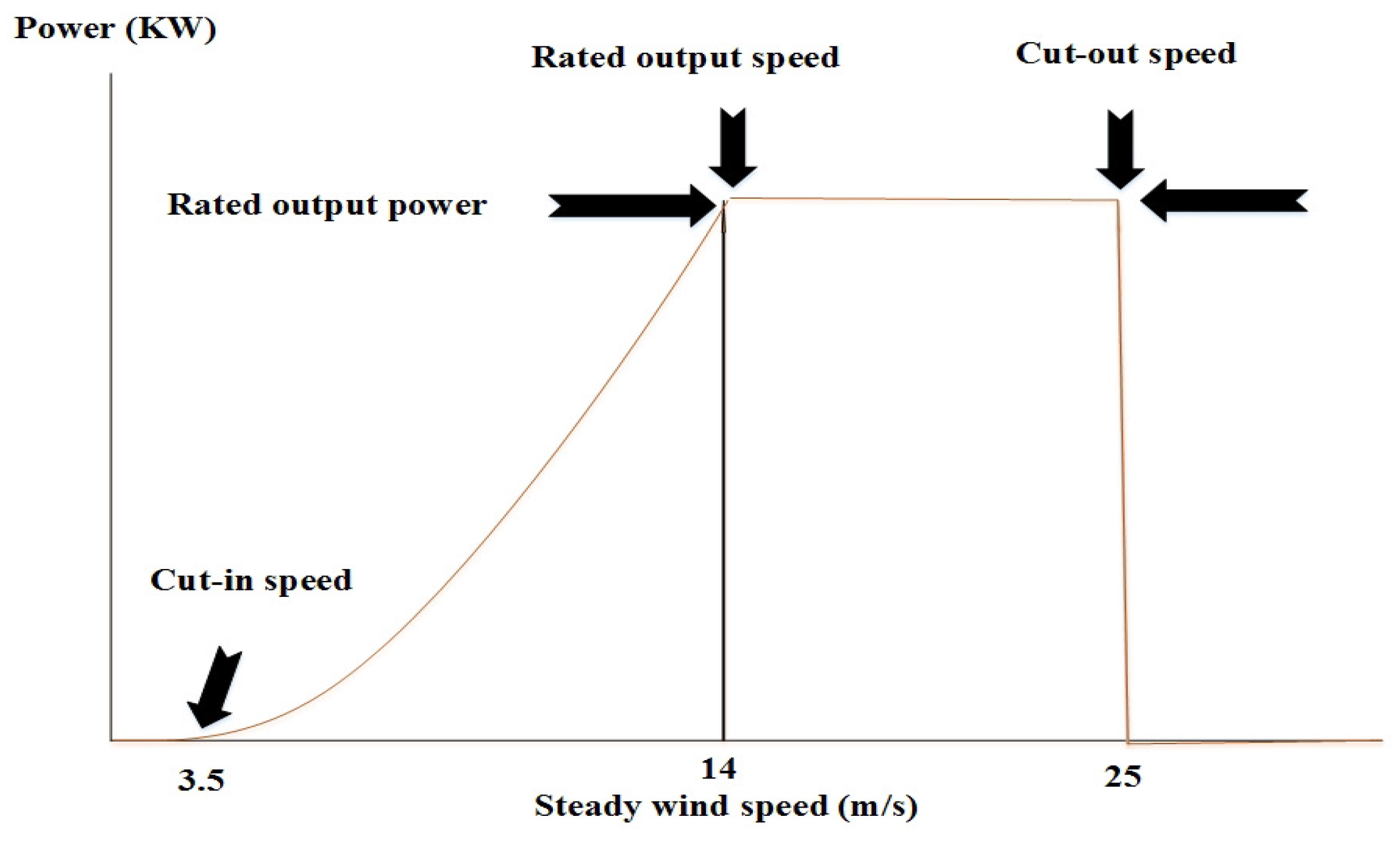
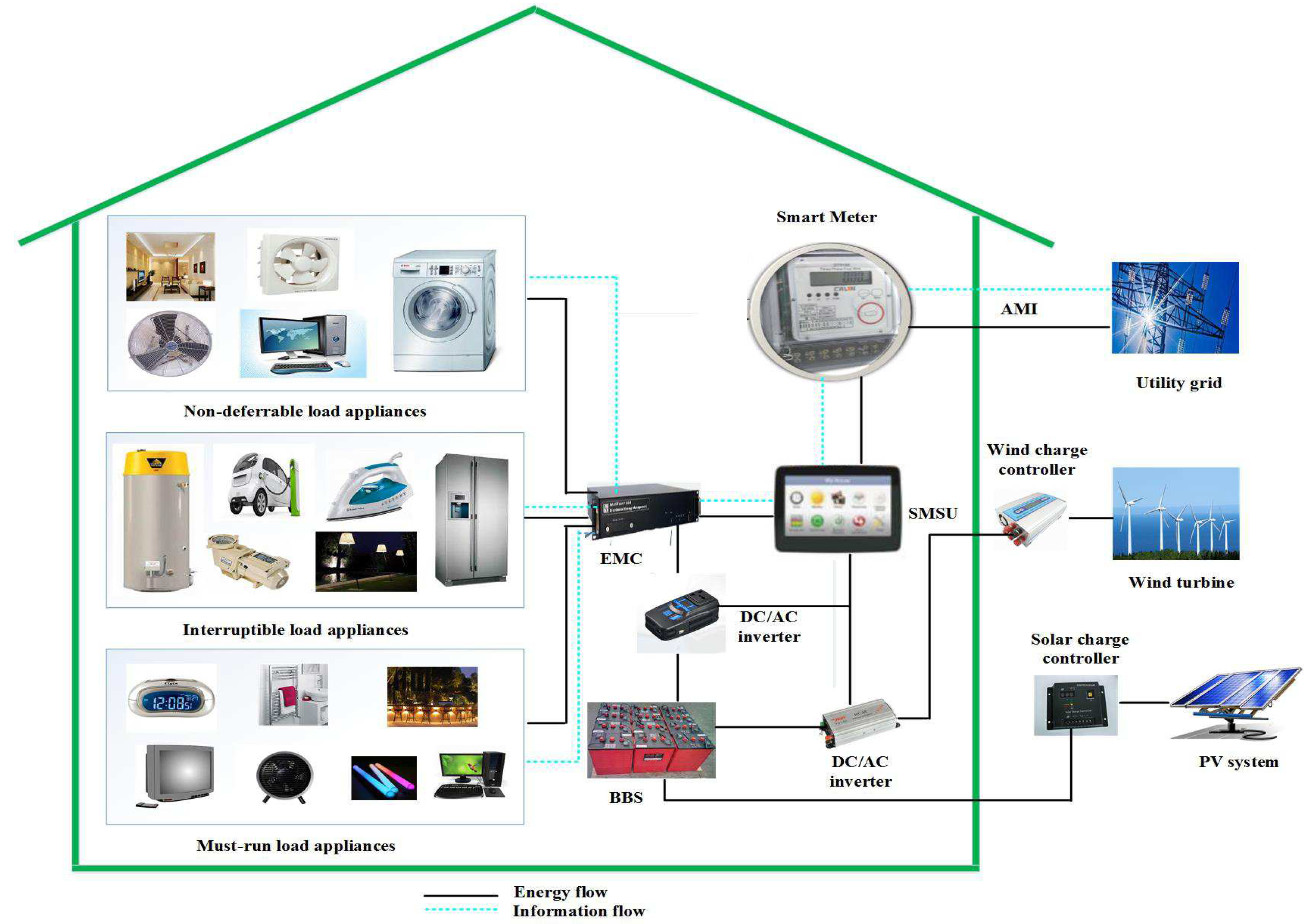
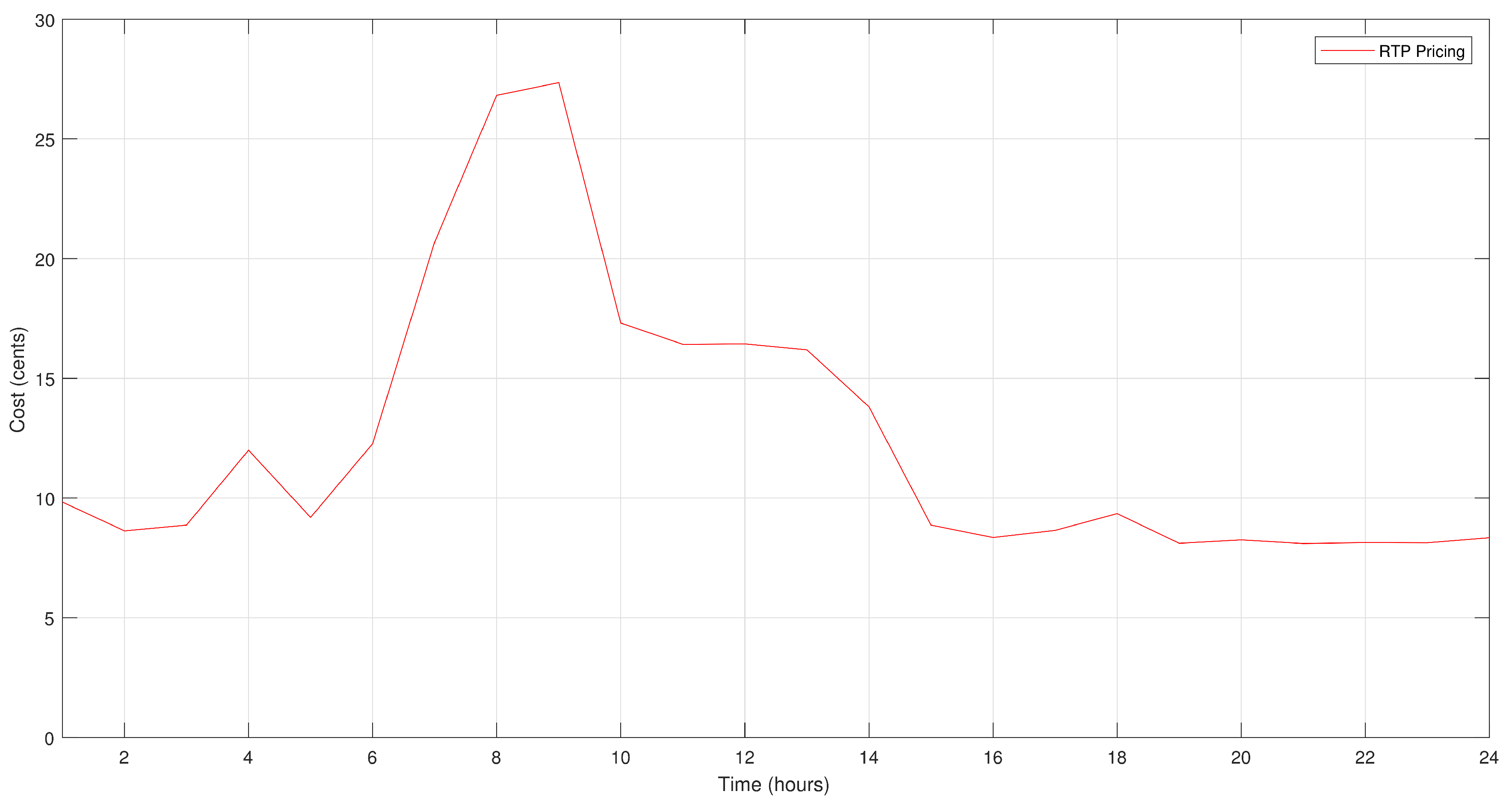
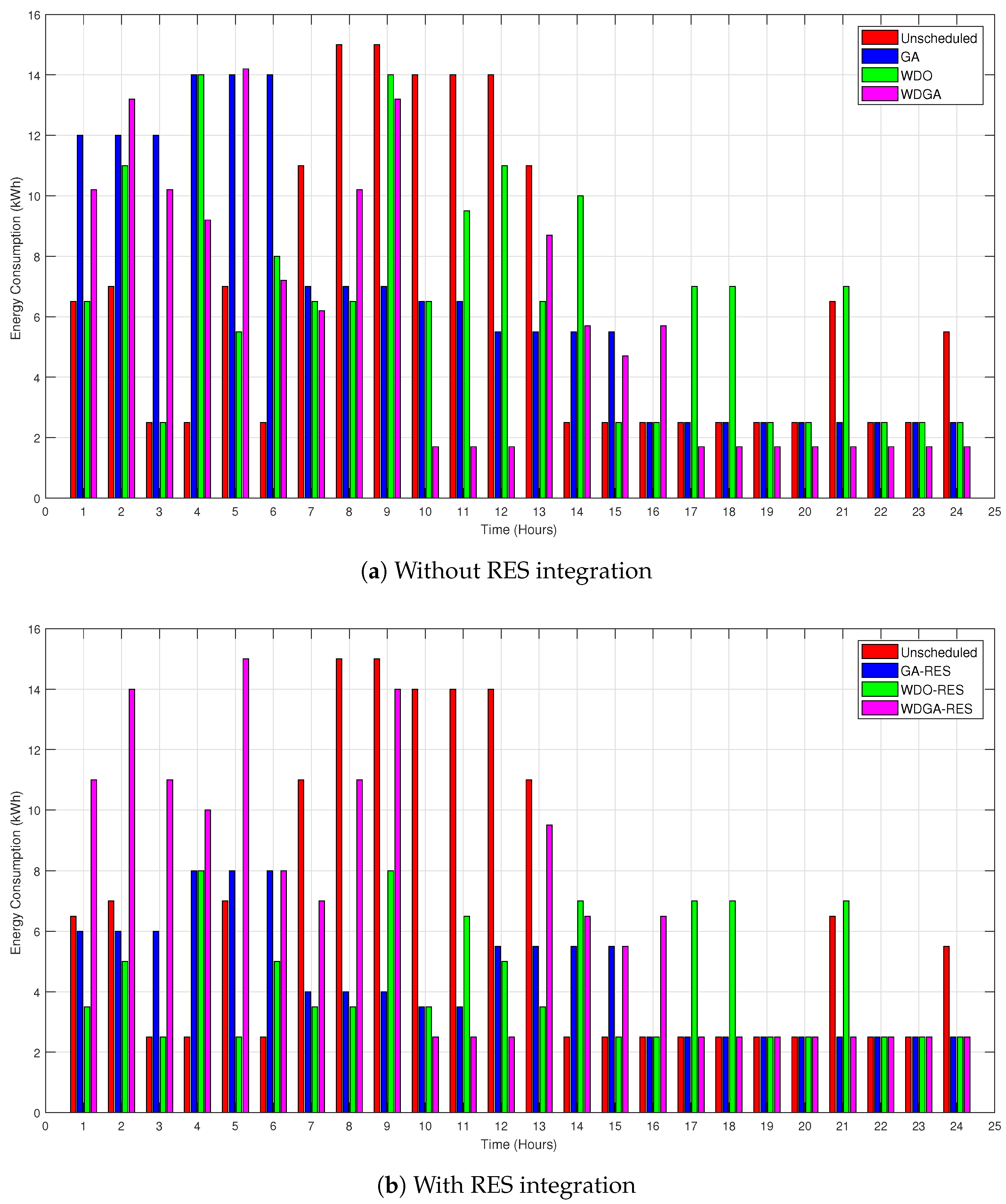
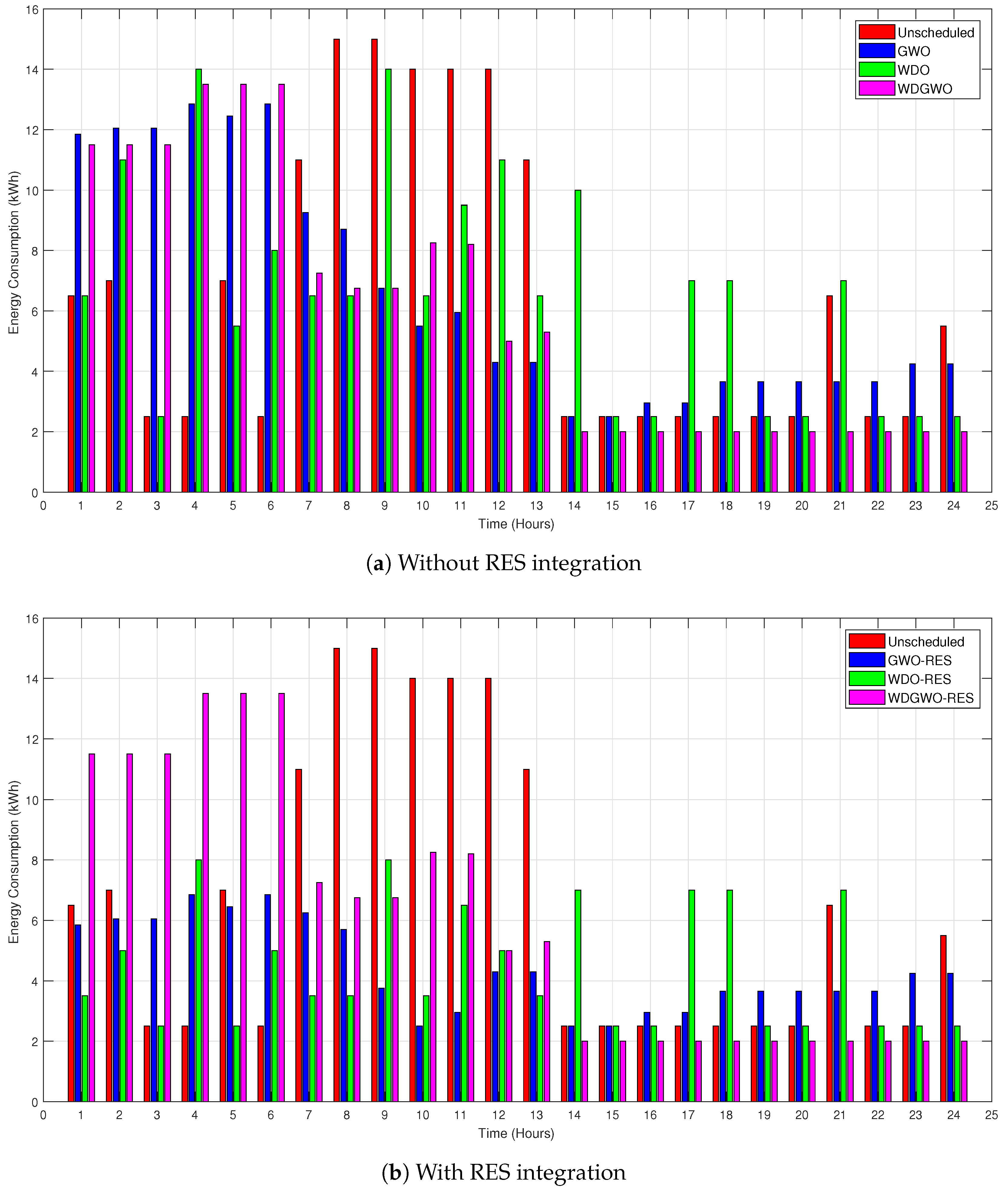
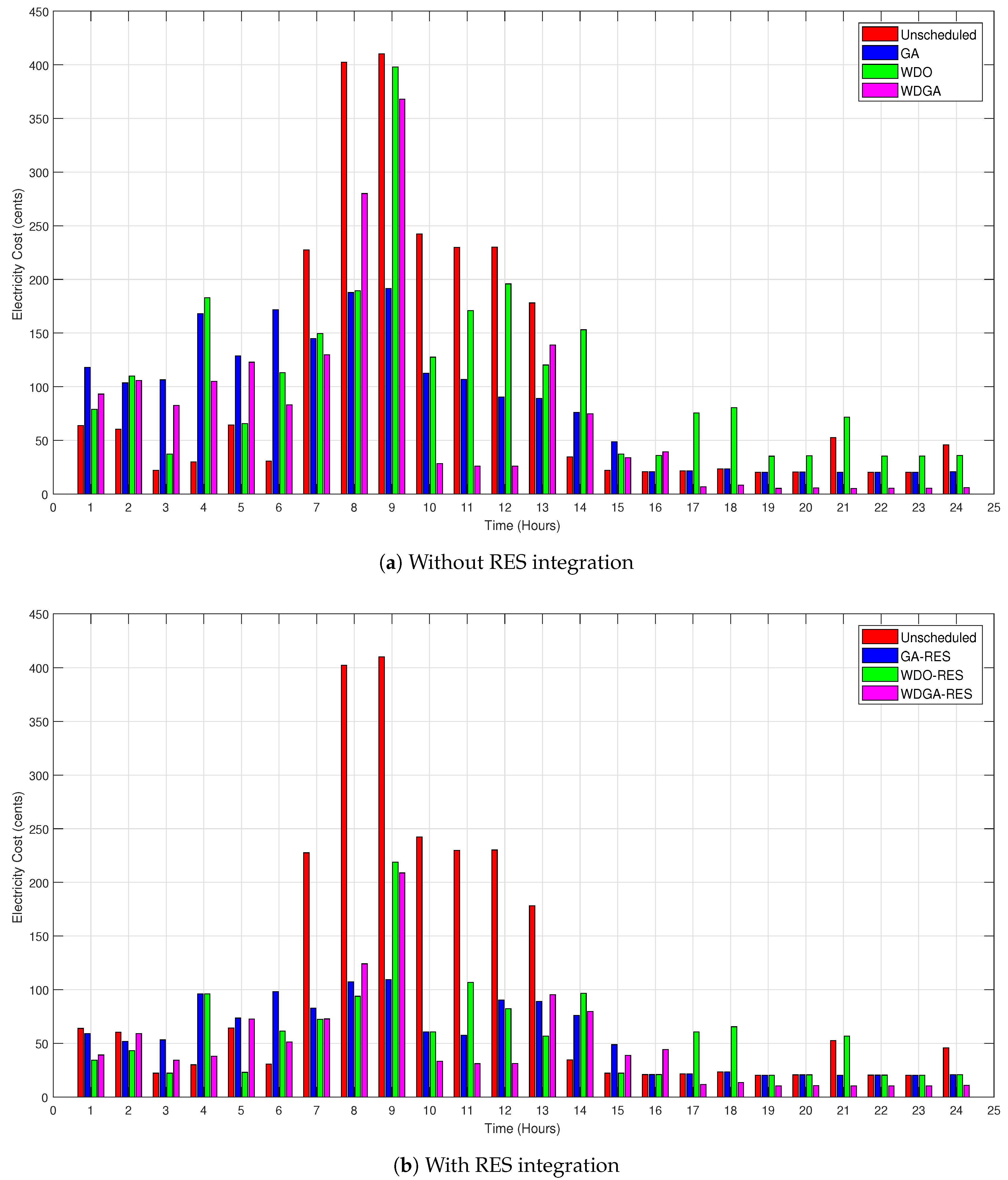
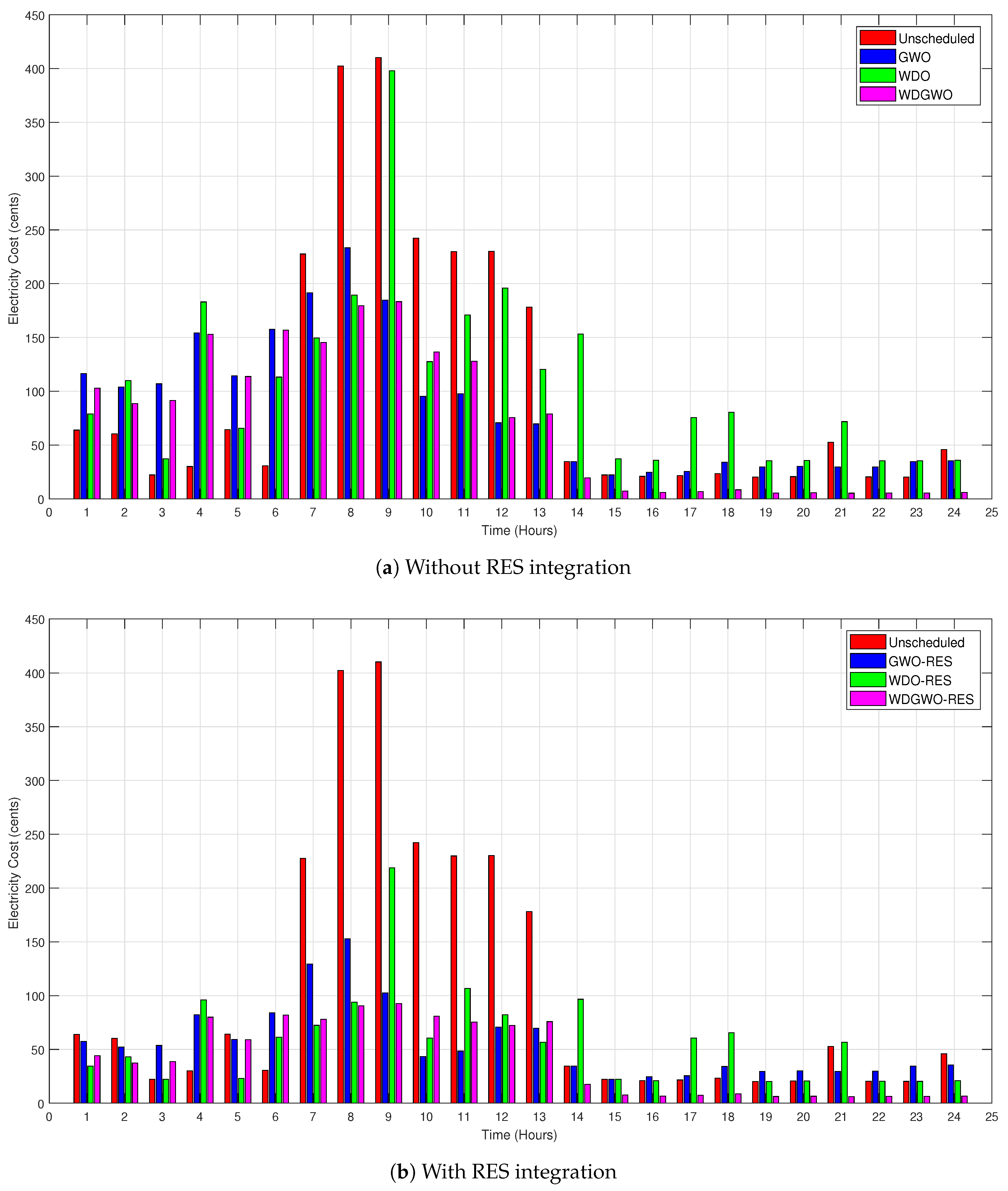
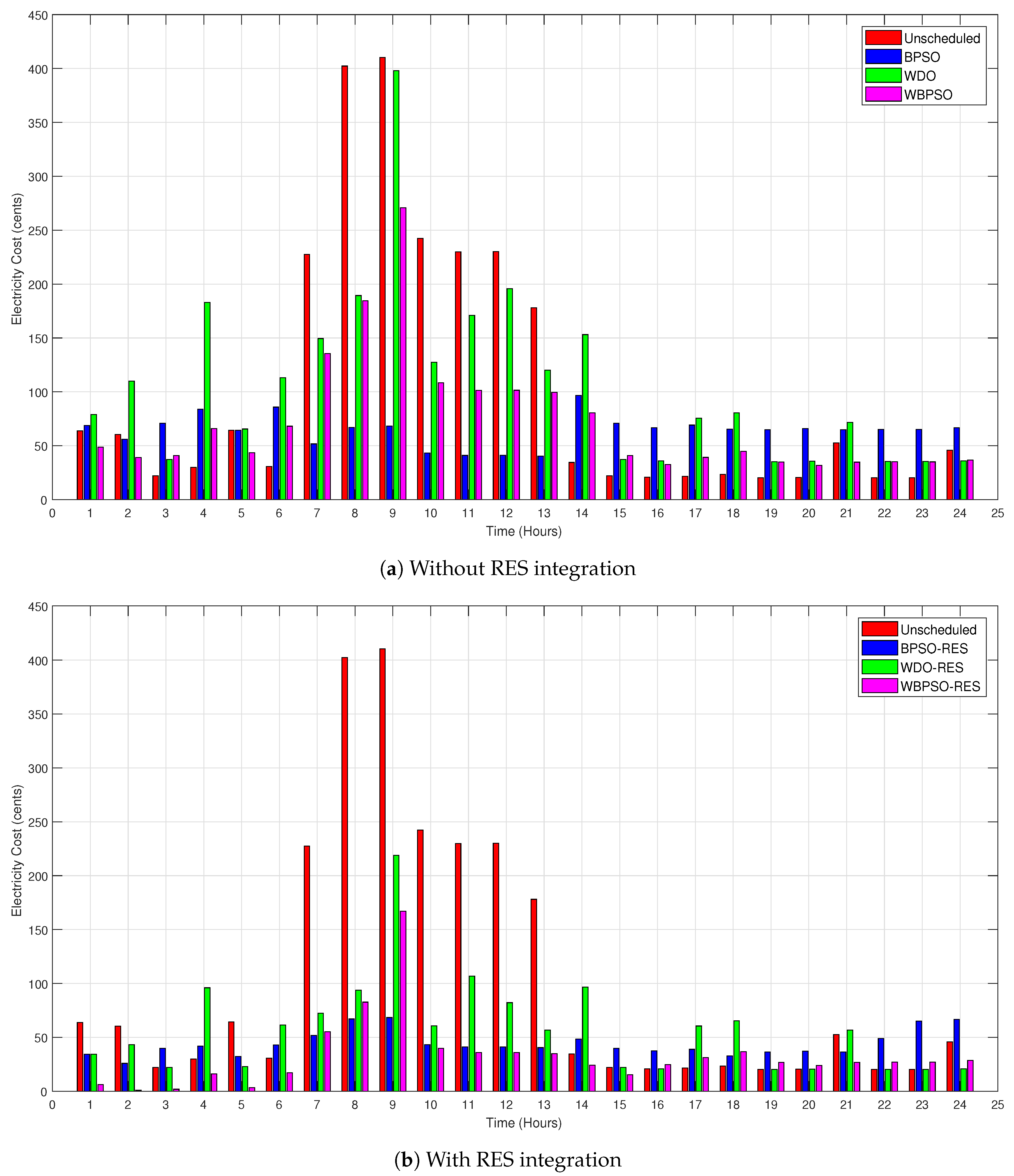
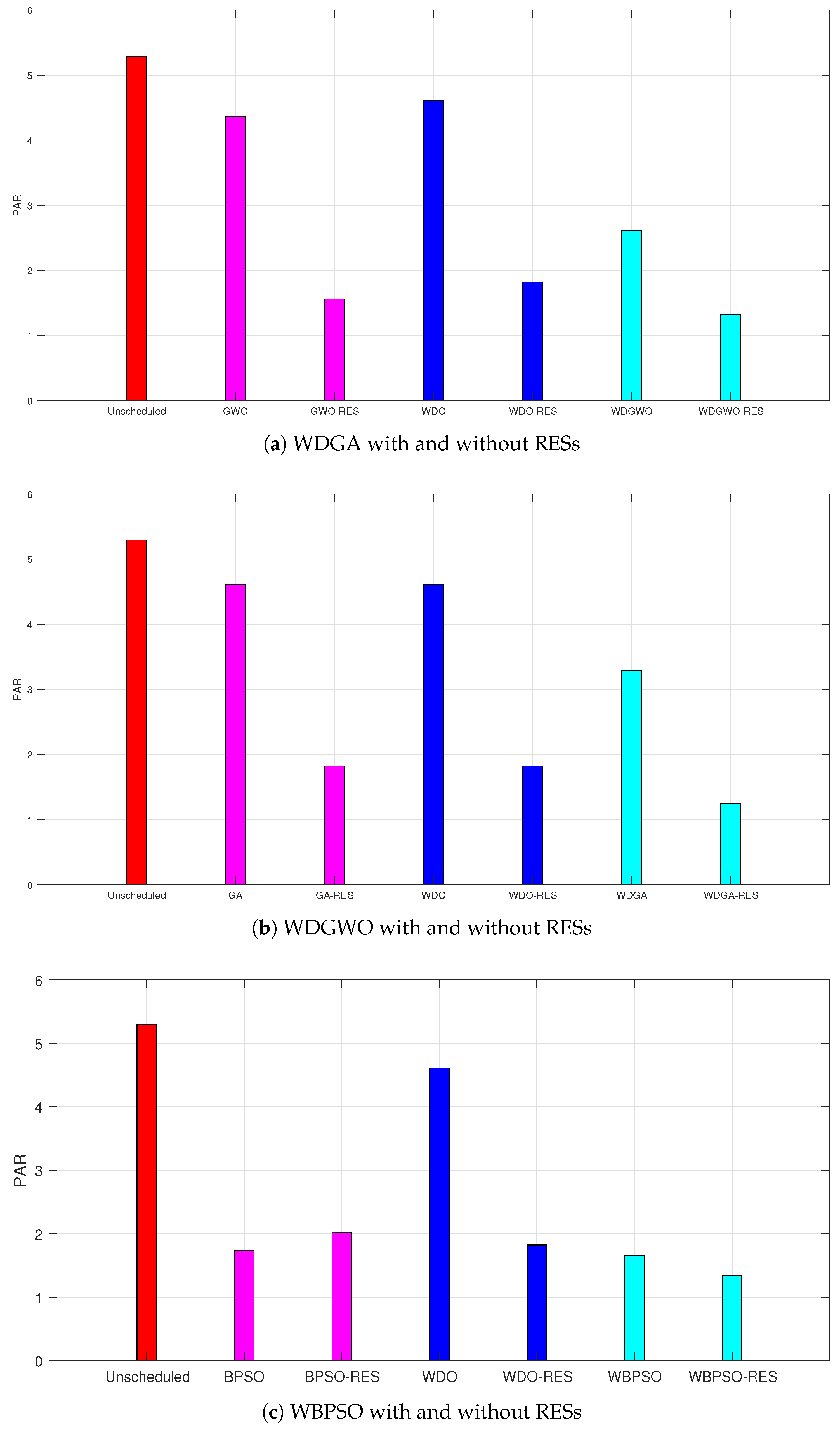
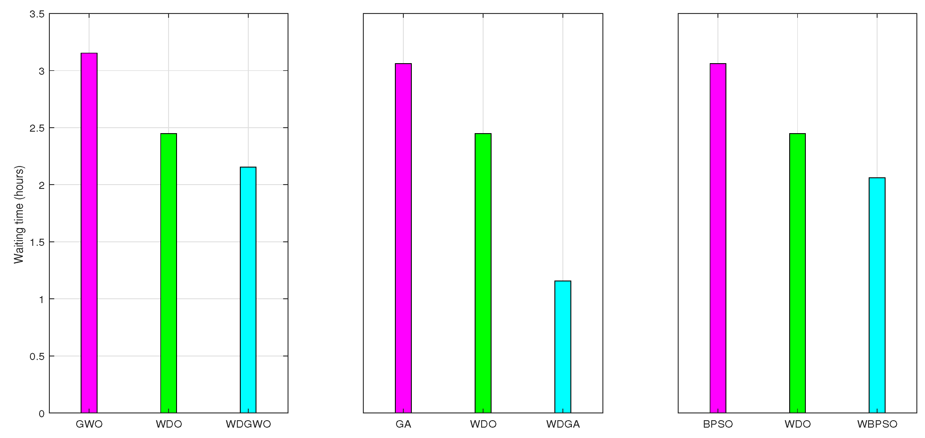
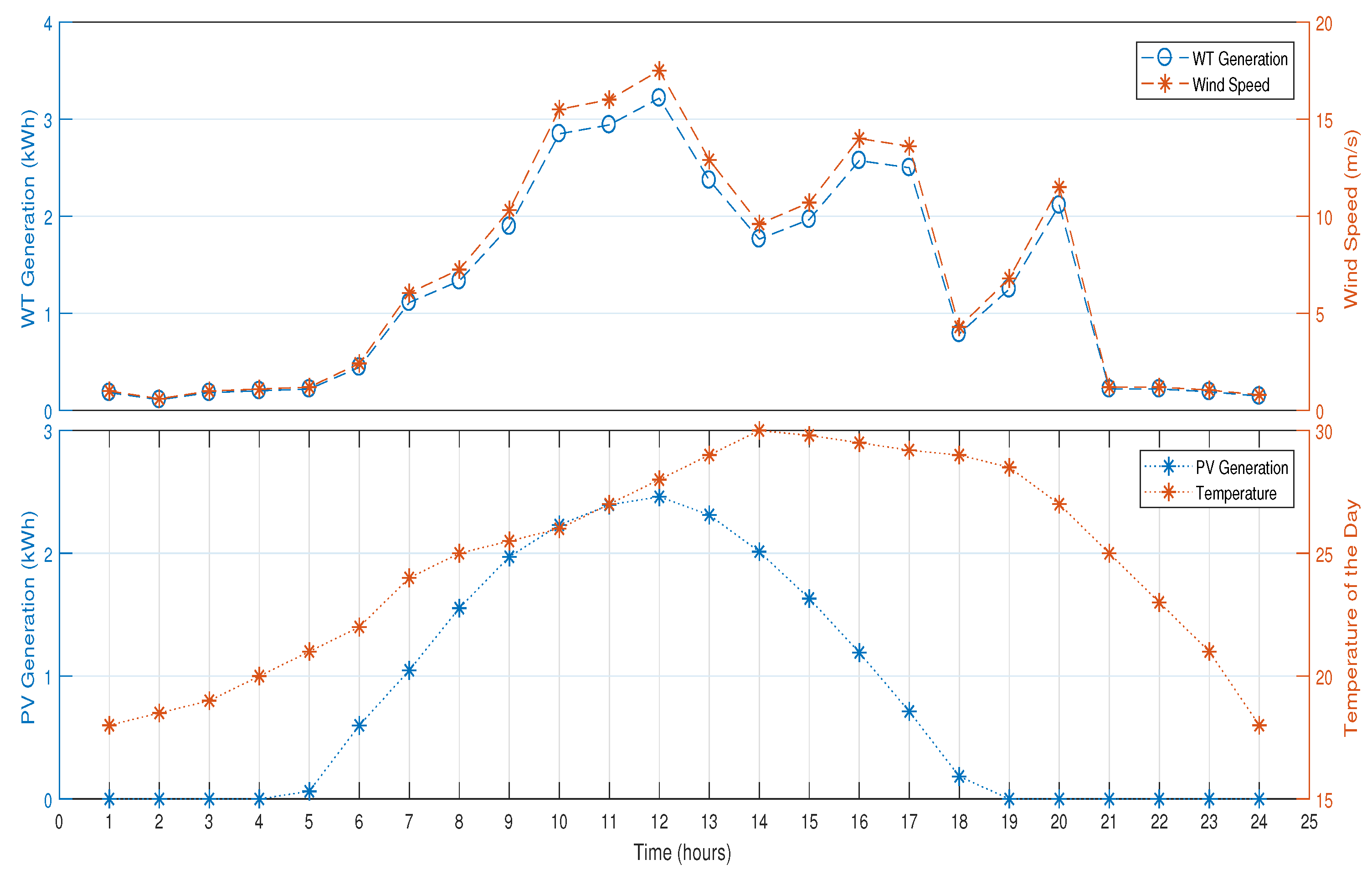
Table 1.
Summarized literature review.
| Technique(s) | Objective(s) | Finding(s) | Limitation(s) |
|---|---|---|---|
| GA [18] | Electricity cost and PAR reduction | Cost and PAR is reduced using RTP and TOU | UC is not considered |
| MILP [19] | PAR and cost reduction with RESs integration | Cost is reduced | Expensive for small scale residential users |
| OCM and MPC [20] | Electricity bill reduction | Optimal energy management solution and cost saving | AWT for UC is not taken into account |
| MIP [21] | Optimal scheduling of energy resources among users | Maximizes energy utilization | UC is not considered |
| SCADA [22] | A hybrid power generation model | Design of hybrid power system | UC is not considered |
| MILP [23] | HEMS modeling and techno-economic sizing | Used single step methodology to size additional PV and ESS | UC and cost reduction are ignored |
| PSO and GA [24] | To minimize electricity cost | Cost is reduced using PSO and GA | To reduce cost UC is compromised |
| MILP [25] | Reduction of emission and cost | emission and cost minimization | UC and PAR are not considered |
| PCPM [26] | Design of a distributed EMS | EMS is designed using optimal operation of microgrids | PAR and UC are not addressed |
| MTPSO [27] | Cost reduction | Cost reduction achieved | UC is not discussed |
| IPSO [28] | Peak load reduction | They achieve desired objectives | UC is compromised and only passive appliances is considered. |
| PMU [29] | To reduce electricity cost | Cost is reduced by peer-to-peer electricity sharing | UC is decreased |
Table 2.
Power rating of system model components.
| Component | Rating |
|---|---|
| Battery | 1.2 kWh |
| Wind turbine | 10 kW |
| Solar panel | 230 W |
Table 3.
Appliances classification.
| Non-Deferrable Loads | Interruptible Loads | Must-Run Loads |
|---|---|---|
| Home lightings | Water heater | Fans |
| Fan | PEV | Optional lightings |
| Exhaust fan | Iron | Heated towel rails |
| Desktop PC | Pool Pump | Personal computer |
| ESS | Refrigerator | Television |
| Washing machine | Out-door lightings | Electric clock |
Table 4.
Parameters of GWO.
| Parameters | Value |
|---|---|
| Total iterations | 50 |
| Population size | 200 |
| 2 to 0 | |
| Random vectors r1, r2 | 0, 1 |
| n | 18 |
Table 5.
Parameters of GA.
| Parameters | Value |
|---|---|
| Number of iterations | 50 |
| Population size | 200 |
| Probability of mutation | 0.1 |
| Probability of crossover | 0.9 |
| n | 18 |
Table 6.
Parameters of BPSO.
| Parameters | Values |
|---|---|
| Number of iterations | 50 |
| Swarm size | 200 |
| Maximum velocity | 4 |
| Minimum velocity | −4 |
| Initial weight constant | 2 |
| Final weight constant | 0.4 |
| Local pull | 2 |
| Global pull | 2 |
| n | 18 |
Table 7.
Parameters of WDO.
| Parameters | Values |
|---|---|
| Total iterations | 50 |
| Population size | 200 |
| dimMin | −5 |
| dimMax | 5 |
| vmin | −0.3 |
| vmax | 0.3 |
| Universal gas constant | 3 |
| n | 18 |
| Gravity | 0.2 |
| Coefficient of friction | 0.4 |
Table 8.
Parameters of WDGA.
| Parameters | Values |
|---|---|
| Number of iterations | 50 |
| Parcels size | 200 |
| Dimensions | [−1, +1] |
| Maximum velocity | 0.4 |
| Universal gas constant | 3.0 |
| Gravity | 0.2 |
| Coefficient of friction | 0.4 |
| Crossover rate | 0.9 |
| Mutation rate | 0.1 |
Table 9.
Parameters of GWDO.
| Parameters | Values |
|---|---|
| Number of iterations | 50 |
| Population size | 200 |
| Dimensions | [−1, +1] |
| Maximum velocity | 0.4 |
| Universal gas constant | 3.0 |
| Gravity | 0.2 |
| Coefficient of friction | 0.4 |
| 2 to 0 | |
| Random vectors r1, r2 | 0, 1 |
| n | 18 |
Table 10.
WBPSO parameters.
| Parameters | Values |
|---|---|
| Number of iterations | 50 |
| Population size | 200 |
| Dimensions | [−1, +1] |
| Maximum velocity | 0.4 |
| Minimum velocity | −4 |
| Initial weight constant | 2 |
| Final weight constant | 0.4 |
| Local pull | 2 |
| Global pull | 2 |
| Gravity | 0.2 |
| Coefficient of friction | 0.4 |
| n | 18 |
Table 11.
Energy consumption with and without RESs.
| Technique | Total Energy Demand(kW) | Imported Energy from Utility (kW) | Difference (kW) | Reduction (%) |
|---|---|---|---|---|
| Unscheduled | 156.5000 | 156.5000 | 0.0000 | 0.0000% |
| GA scheduled | 156.5000 | 156.5000 | 0.0000 | 0.0000% |
| BPSO scheduled | 156.5000 | 156.5000 | 0.0000 | 0.0000% |
| WDO scheduled | 156.5000 | 156.5000 | 0.0000 | 0.0000% |
| GWO scheduled | 156.5000 | 156.5000 | 0.0000 | 0.0000% |
| WDGA scheduled | 156.5000 | 156.5000 | 0.0000 | 0.0000% |
| WDGWO scheduled | 156.5000 | 156.5000 | 0.0000 | 0.0000% |
| WBPSO scheduled | 156.5000 | 156.5000 | 0.0000 | 0.0000% |
| Unscheduled + RESs | 156.5000 | 103.5+53 | 53.0000 | 33.860% |
| GA scheduled + RESs | 156.5000 | 103.5+53 | 53.0000 | 33.860% |
| BPSO scheduled + RESs | 156.5000 | 103.5+53 | 53.0000 | 33.860% |
| WDO scheduled + RESs | 156.5000 | 103.5+53 | 53.0000 | 33.860% |
| GWO scheduled + RESs | 156.5000 | 103.5+53 | 53.0000 | 33.860% |
| WDGA scheduled + RESs | 156.5000 | 103.5+53 | 53.0000 | 33.860% |
| WDGWO scheduled + RESs | 156.5000 | 103.5+53 | 53.0000 | 33.860% |
| WBPSO scheduled + RESs | 156.5000 | 103.5+53 | 53.0000 | 33.860% |
Table 12.
Hourly cost with and without RESs.
| Technique | Cost (Cents/hour) | Difference (Cents/hour) | Reduction (%) |
|---|---|---|---|
| Unscheduled | 103.9500 | 0.0000 | 0.0000% |
| GA scheduled | 84.6842 | 0.0000 | 0.0000% |
| BPSO scheduled | 64.3556 | 0.0000 | 0.0000% |
| WDO scheduled | 96.3625 | 0.0000 | 0.0000% |
| GWO scheduled | 77.9125 | 0.0000 | 0.0000% |
| WDGA scheduled | 83.1125 | 0.0000 | 0.0000% |
| WDGWO scheduled | 71.2750 | 0.0000 | 0.0000% |
| WBPSO scheduled | 73.1100 | 0.0000 | 0.0000% |
| Unscheduled + RESs | 72.8857 | 31.0643 | 42.6205% |
| GA scheduled + RESs | 55.9129 | 28.7713 | 33.9700% |
| BPSO scheduled + RESs | 44.0948 | 20.2608 | 31.4800% |
| WDO scheduled + RESs | 51.5500 | 44.8125 | 46.0500% |
| GWO scheduled + RESs | 53.6400 | 24.2725 | 31.1500% |
| WDGA scheduled + RESs | 54.0355 | 29.0770 | 34.9800% |
| WDGWO scheduled + RESs | 41.2500 | 30.0250 | 42.1200% |
| WBPSO scheduled + RESs | 32.8900 | 40.2200 | 55.0100% |
Table 13.
Total cost of one day with and without RESs.
| Technique | Cost (Cents/day) | Difference (Cents/day) | Reduction (%) |
|---|---|---|---|
| Unscheduled | 2494.8000 | 0.0000 | 0.0000% |
| GA scheduled | 2032.4000 | 0.0000 | 0.0000% |
| BPSO scheduled | 1544.5000 | 0.0000 | 0.0000% |
| WDO scheduled | 2257.7000 | 0.0000 | 0.0000% |
| GWO scheduled | 1869.9000 | 0.0000 | 0.0000% |
| WDGA scheduled | 2174.7000 | 0.0000 | 0.0000% |
| WDGWO scheduled | 1870.6000 | 0.0000 | 0.0000% |
| WBPSO scheduled | 1474.7000 | 0.0000 | 0.0000% |
| Unscheduled + RESs | 1781.0814 | 713.7186 | 40.0722% |
| GA scheduled + RESs | 1341.9000 | 690.5000 | 33.9700% |
| BPSO scheduled + RESs | 1058.3000 | 486.2000 | 31.4700% |
| WDO scheduled + RESs | 1237.4000 | 1020.3000 | 45.1900% |
| GWO scheduled + RESs | 1287.4000 | 582.5000 | 31.1500% |
| WDGA scheduled + RESs | 1196.9000 | 977.8000 | 44.9600% |
| WDGWO scheduled + RESs | 810.0805 | 664.6195 | 35.5200% |
| WBPSO scheduled + RESs | 900.5800 | 574.12000 | 38.9300% |
Table 14.
PAR with and without RESs.
| Technique | PAR | Difference | Reduction (%) |
|---|---|---|---|
| Unscheduled | 5.2915 | 0.0000 | 0.0000% |
| GA scheduled | 4.6095 | 0.0000 | 0.0000% |
| BPSO scheduled | 2.7294 | 0.0000 | 0.0000% |
| WDO scheduled | 5.2915 | 0.0000 | 0.0000% |
| GWO scheduled | 4.2426 | 0.0000 | 0.0000% |
| WDGA scheduled | 3.2915 | 0.0000 | 0.0000% |
| WDGWO scheduled | 2.6095 | 0.0000 | 0.0000% |
| WBPSO scheduled | 1.6518 | 0.0000 | 0.0000% |
| Unscheduled + RESs | 5.2915 | 0.0000 | 0.0000% |
| GA scheduled + RESs | 1.8199 | 2.7896 | 60.5100% |
| BPSO scheduled + RESs | 2.0211 | 0.7083 | 74.0400% |
| WDO scheduled + RESs | 2.5024 | 2.7891 | 47.2900% |
| GWO scheduled + RESs | 1.6265 | 2.6161 | 38.3300% |
| WDGA scheduled + RESs | 1.2474 | 2.0441 | 62.1000% |
| WDGWO scheduled + RESs | 1.3251 | 1.2844 | 49.2200% |
| WBPSO scheduled + RESs | 1.3427 | 0.3091 | 81.2800% |
Table 15.
Effects of wind speed and temperature on wind and PV generation.
| Wind Generation (kWh) | Wind Speed (m/s) | PV Generation (kWh) | Temperature (C) |
|---|---|---|---|
| 0.1838 | 1.0000 | 0 | 18.0000 |
| 0.1103 | 0.6000 | 0 | 18.5000 |
| 0.1838 | 1.0000 | 0 | 19.0000 |
| 0.2021 | 1.1000 | 0 | 20.0000 |
| 0.2205 | 1.2000 | 0.0622 | 21.0000 |
| 0.4447 | 2.4200 | 0.5988 | 22.0000 |
| 1.1111 | 6.0470 | 1.0475 | 24.0000 |
| 1.3331 | 7.2550 | 1.5535 | 25.0000 |
| 1.8945 | 10.3100 | 1.9714 | 25.5000 |
| 2.8481 | 15.5000 | 2.2306 | 26.0000 |
| 2.9400 | 16.0000 | 2.3946 | 27.0000 |
| 3.2156 | 17.5000 | 2.4600 | 28.0000 |
| 2.3704 | 12.9000 | 2.3126 | 29.0000 |
| 1.7640 | 9.6000 | 2.0132 | 30.0000 |
| 1.9661 | 10.7000 | 1.6314 | 29.8000 |
| 2.5725 | 14.0000 | 1.1918 | 29.5000 |
| 2.4990 | 13.6000 | 0.7123 | 29.2000 |
| 0.7901 | 4.3000 | 0.1831 | 29.0000 |
| 1.2495 | 6.8000 | 0 | 28.5000 |
| 2.1131 | 11.5000 | 0 | 27.0000 |
| 0.2205 | 1.2000 | 0 | 25.0000 |
| 0.2205 | 1.2000 | 0 | 23.0000 |
| 0.1929 | 1.0500 | 0 | 21.0000 |
| 0.1470 | 0.8000 | 0 | 18.0000 |
© 2018 by the authors. Licensee MDPI, Basel, Switzerland. This article is an open access article distributed under the terms and conditions of the Creative Commons Attribution (CC BY) license (http://creativecommons.org/licenses/by/4.0/).
Share and Cite
MDPI and ACS Style
Iqbal, Z.; Javaid, N.; Iqbal, S.; Aslam, S.; Khan, Z.A.; Abdul, W.; Almogren, A.; Alamri, A. A Domestic Microgrid with Optimized Home Energy Management System. Energies 2018, 11, 1002. https://doi.org/10.3390/en11041002
AMA Style
Iqbal Z, Javaid N, Iqbal S, Aslam S, Khan ZA, Abdul W, Almogren A, Alamri A. A Domestic Microgrid with Optimized Home Energy Management System. Energies. 2018; 11(4):1002. https://doi.org/10.3390/en11041002
Chicago/Turabian StyleIqbal, Zafar, Nadeem Javaid, Saleem Iqbal, Sheraz Aslam, Zahoor Ali Khan, Wadood Abdul, Ahmad Almogren, and Atif Alamri. 2018. "A Domestic Microgrid with Optimized Home Energy Management System" Energies 11, no. 4: 1002. https://doi.org/10.3390/en11041002
Note that from the first issue of 2016, this journal uses article numbers instead of page numbers. See further details here.