Performance and Accuracy Investigation of the Two-Step Algorithm for Power System State and Line Temperature Estimation


Department of Power Systems, Lublin University of Technology, Nadbystrzycka 38A, 20-618 Lublin, Poland
Energies 2018, 11(4), 1005; https://doi.org/10.3390/en11041005
Submission received: 26 February 2018
/
Revised: 28 March 2018
/
Accepted: 18 April 2018
/
Published: 20 April 2018
(This article belongs to the Section F: Electrical Engineering)
Abstract
:Data concerning actual temperatures of line conductors constitutes essential information for the power system operator. The temperature of the power lines can be used to improve the accuracy of the power system model, thereby increasing the accuracy of the state estimation. This article presents a two-step algorithm for the power system state and line temperature estimation. In its second stage, the proposed method searches for a line temperatures vector, which corrects the uncertain power system base model and allows for further minimization of an objective function. As a result, a more accurate estimation is obtained along with a more precise model of the estimated system. The derived model can then be used for more accurate optimization. The presented method enhances standard procedures of power system state estimation, and its advantage is that it does not require direct measurements performed by phasor measurement units or measurements of line conductor temperatures and weather conditions realized by dynamic line rating systems. The results of simulations made on various test models have been examined, confirming the convergence of the procedure to the point at which the average temperature of the line wires together with the voltage values and phase angles are achieved. The algorithm’s performance and improvement method have also been presented. An advantage of the investigated approach is the possibility to calculate the temperature of line wires with the use of primary measurements in the power system. The presented and examined method, however, is sensitive to the measuring device errors. Additionally, an analysis of the method’s errors and ways of reducing them has been performed.
1. Introduction
Modern power systems should have the possibility of flexible power transmission, which is directly related to the more extensive use of Overhead Transmission Line (OTL) capabilities, especially when it comes to high penetration of renewable energy sources [1,2]. The factor limiting the load of the line is the temperature and sag of the conductors. This depends on many factors, including, among others, the type of conductor, load current, and atmospheric weather conditions [3,4,5,6]. Currently, one of the methods for a more efficient use of the transmission capacity of Overhead Transmission Lines (OTLs) is the installation of precise and cost-intensive Dynamic Line Rating (DLR) systems [7,8,9,10,11,12,13,14]. The aim of the presented method is to estimate the temperature of the line wires, in the absence of weather measurements along the line and with a lack of Dynamic Line Rating (DLR) devices installed in the analyzed system. The method presented in the article enables, in a simplified way, the estimation of the system state and temperature of conductors on the basis of primary measurements of active and reactive powers along with bus voltages. Determining the temperature of the conductors is an element of identifying new parameters of the power system base model, i.e. temperature, resistance, and reactances of the lines. The more accurate corrected model of the power system allows for better, more precise optimization and the obtained solution is closer to the actual optimum. In addition, achieving estimated temperatures of line wires, and thus new parameters of the system model may constitute an element of optimization technique proposed in [15], according to which it is possible to achieve the strict optimum of a non-linear system only if its approximate model is available. A solution that allows for the calculation of the actual average temperature of Overhead Transmission Line (OTL) conductors can be the extension of the power system State Estimation (SE) method [16,17]. The SE of an electric power system is a reasonably well recognized problem and it is often referred to as on-line modeling [18,19,20]. There are many modifications of SE procedure that improve performance [21], the accuracy of results [22] or robustness to the power system model parameter errors [23,24,25,26]. One of the many sources of model parameter errors are the actual OTLs’ operation temperatures [16,27,28,29,30,31,32]. In [16], the authors proposed a two-stage estimation, where at the second stage OTL resistances are updated according to available measurements and actual weather parameters. In [17], the authors proposed a similar algorithm, but they incorporated into the measurement vector four groups of data, where the first group is bus voltage magnitude and branch power, the second group contains measurements from installed Phasor Measurement Units (PMUs), the subsequent group contains the current magnitude measurements, and the last group is comprised of weather-related environment data.
In the present article, a two-step power system state and line temperature estimation is proposed that uses only classical measurements such as active and reactive power, bus voltage and current, without any additional measurements such as ambient parameters from weather stations, conductor temperatures from DLR, voltage and current magnitudes with its angles from PMUs or Wide Area Measurement System (WAMs) [22]. The proposed method assumes a well-identified power system topology, and the absence of bad data measurement values [18]. The accuracy of the temperature estimation method mainly depends on measuring apparatus classes. This approach allows us to determine the OTLs without additional measured values, but it increases the demand for computing power. In this case, the Graphical Processing Unit (GPU) can be used to speed up the estimation calculations. The article analyzes the accuracy of estimating temperature of OTL wires as a function of the measuring instrument classes, along with the estimation times as a function of the size of the power system. A modified listing of MATPOWER [33] code is also presented, one that uses a GPU for performance improvement.
In this paper, the author contributes to analyzing and solving the problem of uncertain power system line temperatures’ estimation, which leads to the more accurate state estimation. The main contributions of this paper are summarized as follows.
- The inaccuracy of the power system model results mainly from the actual temperatures of the operating conductors of the power line, which in the case of accurate measurements causes errors in the estimation of the state. Therefore, a two-stage method for estimating the power system state and line temperatures was proposed. The advantage of the presented algorithm is that it does not require any additional measurement data such as the measurement of current in a line conductor, weather information along the line from DLR systems or PMUs, which can be augmented in measurement function h and measurement Jacobian as proposed in [17].
- A case study based on the IEEE 39 bus New England test system was presented, in which the power line temperatures have been calculated. Based on the achieved results, the two-step algorithm for power system state and line temperature estimation was applied, in order to better understand the algorithm structure and its operation.
- The performance and accuracy of the presented method have been been examined using different test system cases.
- The speed improvement of the presented algorithm estimating a larger power system model has been examined using graphical processing units. The example of modified MATPOWER code for using graphical processing units has been shown.
- The accuracy of the presented method has been examined as a function of instrument transformers classes.
The remaining part of this paper is organized as follows: in Section 2, the classical state estimation procedure is presented. In Section 3, a two-step algorithm for power system state and line temperature estimation is presented, encompassing both theory and implementation. Section 4 is focused on a practical examination of the presented method, its operation, performance and accuracy. Finally, the article is concluded with Section 5.
2. Power System State Estimation
The present-day development of computer technologies makes it possible to perform real-time SE of large and advanced power systems. SE determines the most probable vector of complex voltages using a system model and measured values of bus voltages, active and reactive power of the generation, transmission and loads [18,20,34,35,36]. Additionally, the SE can use current measurements, but their application sometimes causes problems of a mathematical nature [18,19,37], especially when line current is very small. The calculated most probable vector of phase angles and nodal voltages of the estimated system with its model constitutes a basis for the determining of all dependent variables, i.e. power flows and line currents together in metered and non-metered parts of the network. The measured values of the active and reactive power as well as of the voltage and current are characterized by measurement uncertainty [18,37]. That uncertainty mainly follows from the errors of the measuring devices installed in the system. Measurement uncertainty can also result from the resolution of analog-to-digital converters used for signal processing and transmitting the measurement values to Supervisory Control and Data Acquisition (SCADA) computers. Instrument transformers are the source of the greatest measurement errors, but their operating uncertainty is well defined by their classes. Power system SE is most often realized using the iterative Weighted Least Squares (WLS) method. That process takes into consideration the uncertainty of all measured values using the covariance matrix. In an ideal case, when the measured values and the model parameters are not encumbered with any errors, the iterative SE algorithm converges to a strictly optimal point, where the deviation between the estimated and measured values defined as (1) is equal to zero
where -i-th measurement in the PS, —measurement function which is the static model of PS, —vector of the PS state consisting of voltage magnitudes and angles, —deviation between the i-th measurement and the model value. Errors of both the measured values and of the model affect the estimation quality defined by the value of . The State Estimation (SE) uses a static model of the power system, where line resistance values are calculated on the basis of line length and conductor per-length resistances provided by the manufacturer, usually given for the temperature of 20 C. Differences between actual parameters of an operating power line and parameters of a static power system model as a rule pertain to resistance and reactance values and are related to temperature changes in the conductors [16,27,28,29,30,31,32]. Those temperature variations result from the heating effect produced by the current flow and the cooling influence of weather conditions [3,4,38,39].
The theory of the power system State Estimation (SE) [18,20,34,35,36,37] assumes that measured values are characterized by the uncertainty which is defined by Equations (2)–(4) and stands for a standard deviation of the measurement . The measurement uncertainty is the statistically recognized error, consistent with the Gaussian distribution where the function assumes the form:
defined by:
The function f(z) varies depending on the parameters and , and, furthermore, its shape can become standardized with the application of the transformation
where: z—random variable, —mean or expected value of variable , —standard deviation of the variable z.
It is worth noting that the measurement function h is a static model of a power system, where the parameters of its elements such as lines, transformers or shunts can carry an unknown level of uncertainty [18,24]. The SE can be considered as an optimization procedure searching for such a power system’s state vector that makes it possible to obtain the minimum value of the objective function defined as Equation (5):
where: J—objective function, —diagonal weight matrix, while the —covariance of the i-th measurement. The minimum determination of the function J can be verified using the basic first order optimality condition (6):
By expanding (6) into the Taylor series around and neglecting further terms of the series, a basis for iterative calculations is defined (7):
The Gauss-Newton method [18,37] can be applied to obtain a solution for the state vector that minimizes the J function. By transforming Equations (5) and (7) to the differential form, the following formulas can be obtained, respectively:
where: —gain matrix, —solution change in the k-th iteration whereas , —Jacobian determinant of the measurement function is defined as Equation (10):
The SE solution, defined by the vector , can be calculated by solving the for and performing iteration until the condition is fulfilled. Newton’s iteration converges to an ideal solution, that is where , when both the model and the measured values applied to the SE were achieved by solving the task of power system load flow. State estimation of large power systems is computationally demanding because of frequent inversion of the sparse and large matrix . The efficiency of processing can be improved using GPUs.
3. The Concept of the Two-Step Method for Power System State and Line Temperature Estimation
In practical applications of the power system state estimators, the measured values and the static parameters of the power system model contain inaccuracies. These mainly result from the errors in determining the conductor length in the power line, inaccurate manufacturer data concerning conductor resistance as well as resistance vs. temperature dependence [18]. Additionally, the unsteady cooling effect of variable weather conditions along the line route means that the modeled resistance of a line in the power system model does not reflect its actual resistance [25,29,30,31,38]. Furthermore, the variable temperature of the conductors in the line spans brings about variations of the conductor length in spans. This in turn causes changes in the total reactance of the line [30,40], which in some circumstances can be neglected [32,39]. In such a case, the error part of Equation (5) assumes the form where the measurement function depends both on the vector of state variables and on the vector of model parameters . In a typical State Estimation (SE), the vector of the model parameters remains constant:
where: —i-th measurement in the power system (PS), —measurement function, —vector of the PS state, —parameters of the PS model, —deviation between the i-th measurement and the model value or absolute accuracy [18].
In practice, measurement values acquired by the SCADA systems which constitute the basis for the estimation, are never ideally synchronized and are encumbered with measurement errors. Assuming that the measurements are realized in the steady state condition, the question of non-synchronous measurements can be neglected. In such a case, it can be stated that a static model of a power system is encumbered with errors following the modeling inaccuracies and from the actual operating conditions. As described above, the classical SE [18] assumes that the system model is well recognized and does not need any adjustments, which can eventually yield incorrect estimation results, even if the applied measured quantities are accurate [30,41].
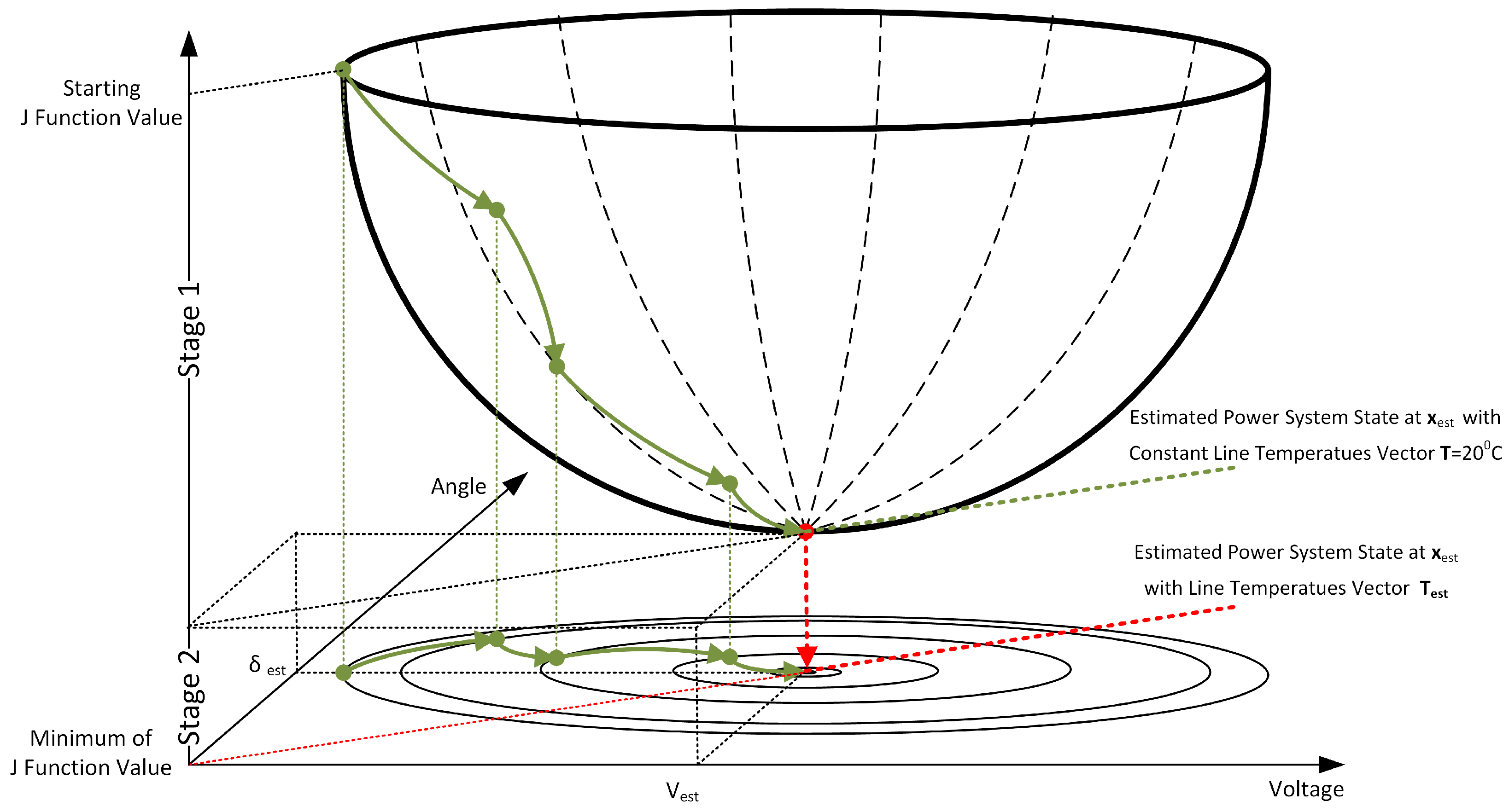
The state of the power system and selected model parameters, e.g., line temperature or resistance, can be estimated in a two-stage process, where the objective function assumes the form:
and in the first stage the classical power system SE takes place, whose aim is to minimize J (12) incorporating the condition. The solution of the first estimation stage produces a vector. In the second stage, the objective function J gets the form:
and is further minimized where for the searched vector , the is calculated minimizing J. In the second stage, the model parameter vector is finally achieved if the minimum condition of the J function is met. At the end of the presented procedure the power system state vector and model parameter vector is obtained. In such a situation, it can be assumed that the model parameter vector is equal to the vector , which stands for temperatures of lines in the power system. The Equation (13) assumes the final form:
where, analogously, the minimization of J as a function of leads to the estimation of the vector of line temperatures and . The illustrative example of the two-stage method for power system state and line temperature estimation has been presented in Figure 1.
3.1. Incorporation of Estimated Line Temperatures into Power System Model
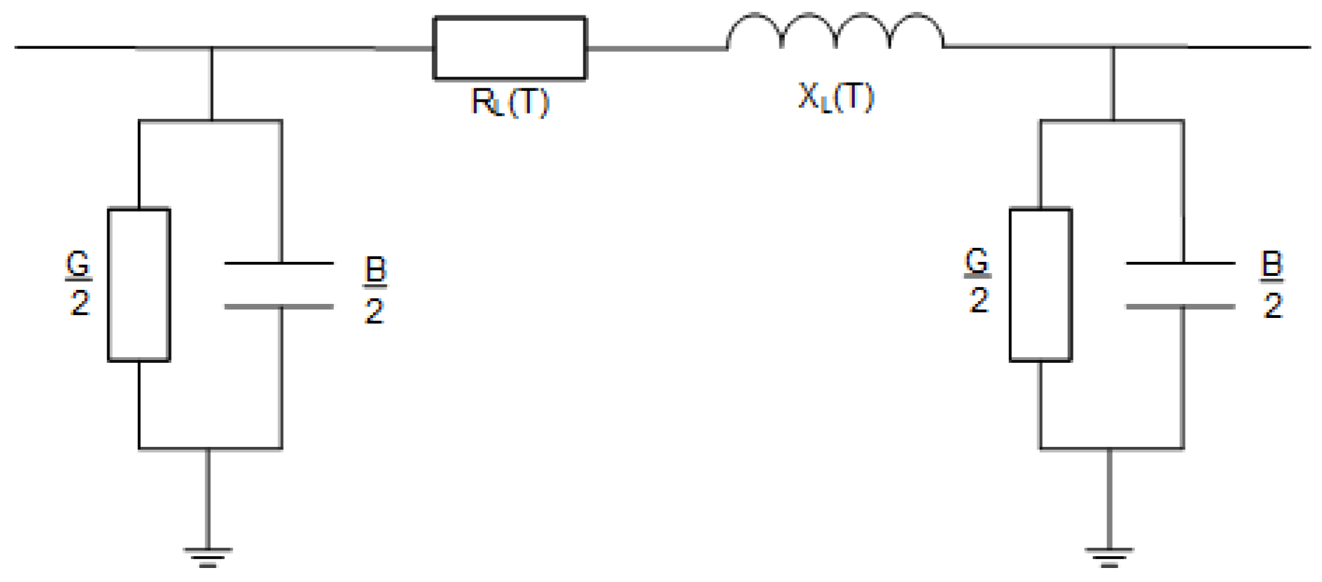
In the models of an electric power system that are used for the load-flow and estimation calculations, a power line is usually modeled in the form of a quadripole (Figure 2), where the line resistance and reactance are lumped parameters. In the present article, it has been assumed that the parameters and vary with conductor temperature. The base values of and are calculated using the well-known dependences [18,19,20] and are determined on the basis of the actual length of the line and its per-unit length parameters. Conductors resistance per length unit is given by their manufacturer and it is usually specified for the temperature of 20 C [41], while the per-unit length reactance is determined as a function of the pole geometry, voltage levels and other acknowledged parameters [19,20,31]. The temperature of the conductors affects conductor resistance while thermal expansion affects their length, which implies changes in total line reactance. In such a case, it can be stated that the line reactance becomes temperature-dependent , as shown in Figure 2 [16,30].
In the case of a 110 kV line, the total line conductance G and susceptance B (Figure 2) can be considered to be constant at low humidity of the atmospheric air and in some cases can be neglected. Furthermore, it has been assumed that the values B and G are constant. Following [30,38,39], equivalent resistance and reactance of an overhead transmission line can be written as follows:
and
where: , —equivalent line resistance and reactance calculated for the temperature of 20 C, respectively; —temperature coefficient of the conductor resistance changes dependent on the conductor type assumed that = 0.00403 for ASCR 7/26; —temperature coefficient of the line reactance change, considering the line expansion effect, according to [30], it has been assumed that , T—actual temperature of the conductor, C—base temperature used to determine and . In the case of the High Temperature Low Sag (HTLS) conductors, the assumption that is invalid and should be corrected [31]. The temperature of the overhead line conductors according to [3,4,31] depends on the conductor design, geometry and the applied materials, which mainly translates into conductor resistance given by the manufacturer as the parameter. Resistance also depends on the atmospheric conditions such as air temperature, wind direction and speed, along with solar radiation.
3.2. Implementation of the Two-Step Algorithm of Power System State and Line Temperature Estimation
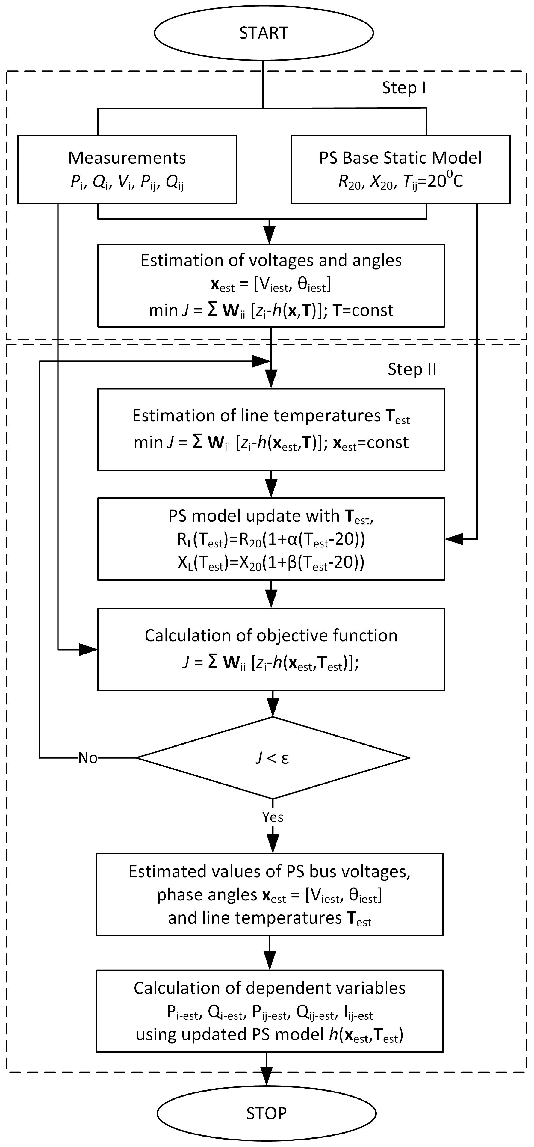
According to the theory of power system SE [18,19,34,35,36], the iterative Newton-Raphson procedure applied to minimize objective function (5) leads to a strictly optimal solution of , where the objective function (5) , when there are no errors in either the model or the measured values. In an ideal case, the model and measurement values are taken from the load flow solution. In practice, however, both the measured values and the model of the estimating system contain errors. In such a situation, the SE usually yields the result where the objective function (14) . The calculated state vector is a suboptimal solution with respect to the real state of the power system (e.g., power line conductor temperatures are different than 20 C) [41]. The estimation quality can be intensified by the application of a more accurate measuring apparatus coupled with the accuracy improvement of the power system static model. The impact of the power system model accuracy on the results of the power system SE has been analyzed in [16,18,41]. Assuming that accurate and error-free measurements in the power system are available, and in order to meet the condition, it is necessary to update the base model with line conductor temperatures. At the same time, conductor temperature influences the mechanical condition of the lines, such as the sag which translates into total line reactance [30,40,42,43]. In such a case, in order to improve the estimation quality and thereby determine the most probable state of the power system together with the estimation of the actual line conductor temperatures, a two-step algorithm for the state and temperature estimation of the power system model can be applied. The method theoretically presented in Section 3 can be implemented as shown in Figure 3, where , —total active/reactive power of the generation and loads in the i-th node of the network , —voltage in the i-th node of the network, —measured power flows in the network branches between the i-th and the j-th nodes. The steady-state condition of the observed power system is assumed, which implies that thermodynamic heating of the conductors and their sagging proceeds slowly.
The realization of the proposed estimation algorithm (Figure 3) is being processed in two stages, as presented schematically in Figure 1. In the first stage, classical estimation of the power system is performed based on the available system model and the measurement data, according to (14). The base system model is where the resistance and reactance parameters of all the power lines are determined for the temperature of 20 C, as [18,20,37,44] argue.
The second stage of the algorithm realization (Figure 3) includes the iterative Newton-Raphson procedure loop, searching for a vector composed of the temperature values of individual power lines to be used to adjust the R and X parameters in the model. It starts from the vector , where all temperature values are equal to 20 C and then performs a sequential estimation-optimization procedure to find such a vector for which the J indicator is minimal. Next, the objective function J’s value is analyzed to check whether the condition is met. If the condition is not met, it means that the power system model parameters should be corrected with new power line temperature values different from 20 C in order to minimize J (trying to minimize J more). The determined temperature of the power system lines is the average line temperatures determined on the basis of the values of electrical quantities measured at the line ends. Furthermore, it can be observed that such an approach makes it possible to estimate the line conductor operating temperature without performing any additional meteorological measurements along the line, such as conductor temperature resulting from weather conditions and the current flow [10,17,45], which directly affects the measured electrical quantities. One disadvantage of this approach is that it does not offer any information on the temperature of individual sections of a power line, whose cooling by the wind can vary due to their varied position with respect to wind direction [3,4].
4. Test System Simulation and State with the Line Temperatures Estimation
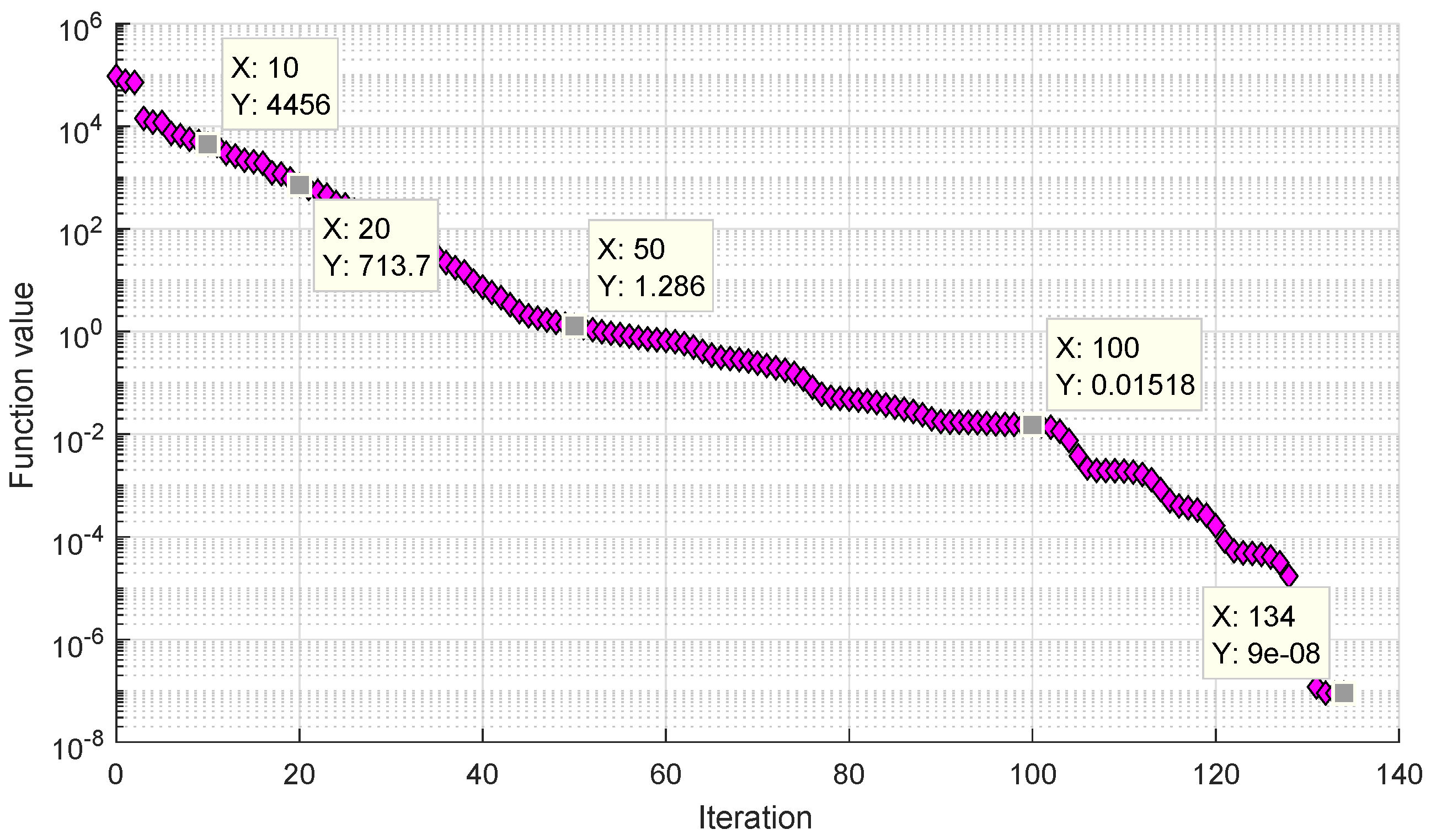
For the purpose of method testing, the IEEE 39-Bus New England Test System, has been used [33]. The length of all lines had been estimated on the basis of specific resistance for 795 kcmil 26/7 Drake ACSR conductor connected as two-bundle, resulting line resistance 0.03585 /km at temperature C. For specific weather conditions used for calculation of conductor temperatures in summer and winter case, the author refers to data presented in Appendix A and in Table A1. The power flow calculations using Electro-Thermal Overhead Line (ET-OHL) model have been performed as in [32]. Next, from the power flow results, the values of active and reactive powers along with bus voltages (P, Q, V) have been used for the power system state and line temperature estimation method. As described in Section 3.2, these values represent the actual measurements acquired by SCADA from Remote Terminal Units (RTUs) and Intelligent Electronic Devices (IEDs). At the first stage of the presented method, the classical SE uses actual measurements with power system base model, containing line resistances calculated for C, as presented in Table A1. The first step of the presented estimation method leads to the J = 94,693.7034 value, assuming that for every single measurement available. The IEEE 39 Bus New England Test System state estimation results compared to the available measurements, after the first step of the processing method, have been presented in Table A2, Table A3 and Table A4, where – stands for active and reactive powers at the beginning of the line, analogously – stands for active and reactive powers at the end of line as well as – which are the active and reactive powers produced by generators. The following second stage of the presented methods uses previously measured values. At the second stage, we perform further minimization of the J function, searching for line temperature vector . The upper and lower bounds for every element of vector have been set to C and C, respectively. The line temperature estimation results and values of the objective function J after 10, 20, 50, 100, 134 iteration have been presented in Table A5 and in Figure 4.
4.1. Algorithm Performance Testing and Timing Results
The testing of the two-step algorithm presented in Figure 3 for its performance and convergence has been performed based on the available power system test models IEEE 9, 14, 30, 39, 57, 118 and 300, with the application of the MATPOWER (version 6.0, PSERC, Tempe, AZ, USA) [33]. For performance testing of the presented method, the lines’ resistances and reactances of used test systems have been calculated for C.
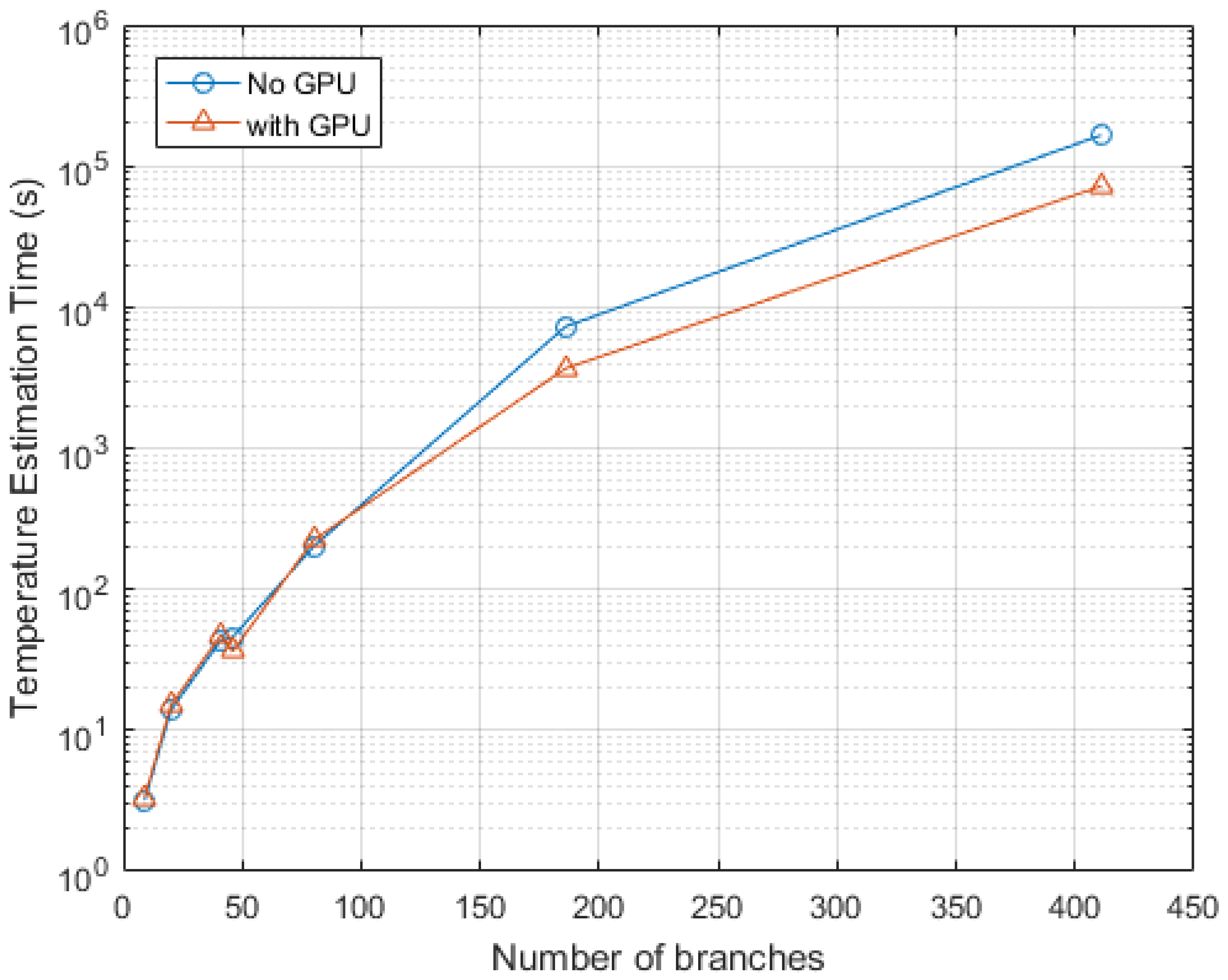
The proposed method makes it possible to determine average temperatures of power lines, but with the increasing number of nodes and power lines the procedure realization time gets significantly longer. The notable elongation of temperature estimation time results from several features. The growing complexity of the power system model entails an increased number of iterations in a single system state estimation and calculation of objective function J. The growing number of lines increases the number of elements in the temperature vector , and thus the number of estimations per one change of the vector increases exponentially. The state and line temperatures estimation needs to be performed as soon as possible for the purpose of the usability of results. During the simulation tests, it turned out that the three most computationally costly operations in the estimation process are: (1) Jacobian calculation , where -measurement Jacobian, -covariance matrix; (2) Calculation ; (3) Calculation of step change . In order to speed up the estimation calculations, the above matrix operations have been implemented to perform using the GPU. An example of a modified MATPOWER®software code for performing Graphical Processing Unit (GPU) calculations is shown in Algorithm 1.
The simulations and estimations have been performed using a benchmark machine Fujitsu PRIMERGY TX300® Server (version S6, Fujitsu Technology Solutions GmbH, Munchen, Germany) equipped with two Intel Xeon®E5-2690v2 3.0 GHz processors (acting as 20-core CPU) (Intel, Santa Clara, CA, USA) and 192 GB RAM (Fujitsu Technology Solutions GmbH, Munchen, Germany), operating under Microsoft Windows 2012 R2 with and without the Graphical Processing Unit (GPU) (NVIDIA Tesla K40, Santa Clara, CA, USA) support for estimation purposes. The results have been presented in Table 1 and Figure 5. All the tested cases have shown the algorithm’s convergence to a strictly optimal point using the complete and correct set of measured data, which is a set of values obtained from the load-flow solution. In the case of small systems, transferring the matrixes and many times from RAM to GPU and vice versa (), as shown in Algorithm 1, effects in a more extended total temperature estimation time. The performance improvement is noticeable in the case of larger systems, where and have a larger dimension and computing of , and is faster on GPU than on CPU.
| Algorithm 1: Modified code of MATPOWER [33] State Estimation (SE) function doSE.m for performance improvement using Graphical Processing Unit (GPU). |
| ... |
| % --compute inverse R matrix on GPU |
| R_inv = gpuArray(diag(1./sigma_square)); |
| ... |
| --construct H matrix on GPU |
| H = gpuArray(H); |
| %--compute update step on GPU |
| J = H’*R_inv*H; |
| %--evaluate F(x) on GPU |
| F = H’*R_inv*(z-z_est); |
| %--compute dx on GPU |
| dx = (J / F); |
| %--get matrix from GPU |
| dx = gather(dx); |
It is worth noting that the presented method can be used to analyze operating system state and line average temperatures ex-post, due to the long calculation time for large systems as shown in Table 1. Similar calculation times can be found for power systems optimization with the application of heuristic methods. In [17] the Authors proposed state and line temperature estimation method that finished calculations of IEEE 57 bus test system in 3.29 seconds in single estimation, while the presented technique needs 201.04 seconds. It is inducted by the fact that presented method runs as two iterative steps. The second step, which is a classical state estimation occurs many times because it does not include any additional measurements incorporated into measurement function h and measurement Jacobian as in [17].
4.2. Temperature Estimation Error Analysis Using Complete and Incomplete Sets of the Noise-Containing Measured Data
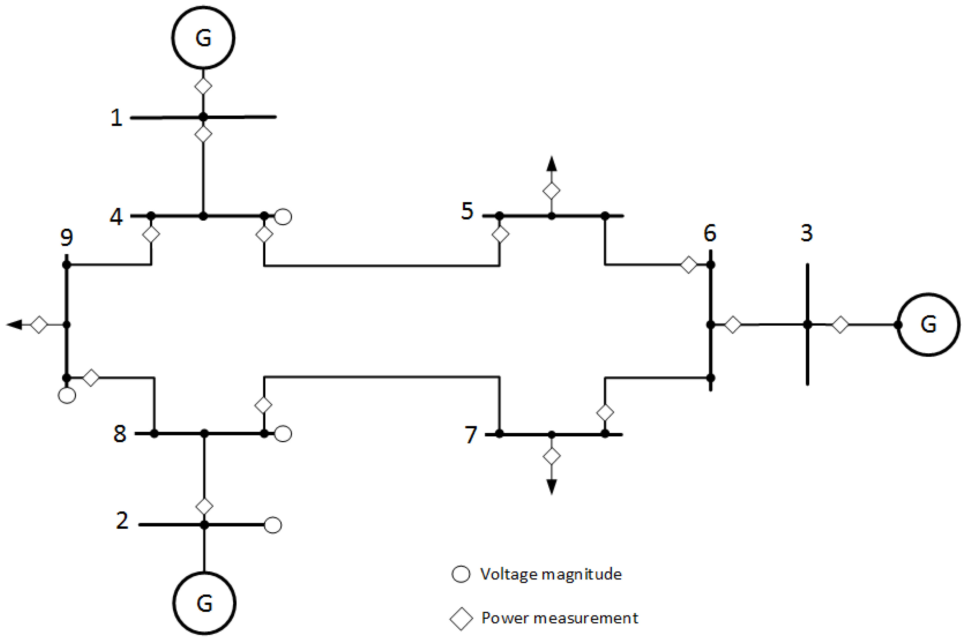
The convergence, errors and sensitivity of the algorithm have been analyzed for the case of an incomplete and noise-containing set of measurement data with the application of a modified IEEE 9 bus test system presented in (Figure 6) where all line temperatures have been assumed as C. The relative error and mean relative error of the presented method have been calculated according to Equation (17).
The algorithm testing has been performed for two different cases. The first one assumes the availability of a complete set of measurement data in the test system, which means that the measured values of the bus voltage V in all the nodes as well as the measured values of active P and reactive power Q in each line and at generator circuit breaker cubicle are available. Noise has been added to the measured values obtained from the load-flow solution in accordance with the statistically assumed normal error distribution following from the instrument transformer classes (0.1, 0.2 and 0.5) [18,20,37]. In the test system, ten thousand samples have been produced. For each of the measurement sets, the two-step algorithm for the system state and line temperature estimation has been realized. The testing objective has been to check the procedure’s operation in the conditions where measurement errors occur that simulate the real system operating conditions. In general, the accuracy of the method is conditioned by the accuracy of the deployed measuring apparatus. Preliminary analysis of the gathered results shows that the discussed method of the estimation of line conductor temperature is very sensitive to measurement errors. Even small errors produced by the measuring apparatus can cause considerable temperature value deviations from the real values. Thus, single measurements (singular snapshots of the system) can yield unreliable results.
The accuracy of the method can be significantly improved by averaging measured or estimated values over an adequate time interval, e.g., over one minute at a varied sampling frequency, that is the frequency of taking snapshots. The time constant for the heating of power line conductors varies between 5–15 min depending on the actual weather conditions [3,4]. Therefore, the averaging interval of 1 min has been assumed. Table 2, Table 3 and Table 4 present data on the method accuracy obtained for the case using a complete measurement data set of the test system shown in Figure 6. An analysis of the results makes it possible to assess the accuracy of the system’s state and line conductor temperature estimation in the case when a complete measurement data set is available.
The results of the algorithm’s application show that the discussed temperature estimation method is very sensitive to the measurement errors of the active P and reactive Q power. Even small measurement errors can yield high mean errors in the estimated line conductor temperature values, even up to 52.5% in the case of single snapshots.
We also tested the method’s accuracy for an incomplete set of the measured values. Figure 6 presents the measurement data that are available in the test system, for which the observability condition is met. In the case of a complete dataset, 57 values of P, Q and U are available, while the incomplete case offers 34 values, which makes almost 60% (exactly 59.65%) of the measurement data available in the complete case. Table 5 and Table 6 present the results of conductor temperature estimation as a function of the deployed instrument transformer classes and sampling frequencies at the 1-min averaging interval for the case of a limited availability of the measurement data. However, in the case of multiple sequence measurements and estimations performed and followed by the determination of an average line temperature value, the mean error of temperature determination is reduced to below 5% (with the application of the 0.5 class measuring apparatus), which for the power line design temperature values yields the limiting values given below in Table 7 and mean values listed in Table 8.
5. Conclusions
Based on the performed testing of the two-step power system state and line temperature estimation algorithm and the gathered results, the following conclusions can be drawn. State estimation of an electric power system is performed based on measurement data encumbered with errors. A power system model that is used for the estimation purposes also deviates from real parameters, because of the applied simplifications and modeling errors. However, the main source of parameter deviations are operating factors, such as heating of line conductors, which affects the resistance and reactance of power lines. The power line monitoring is mainly realized in specific spots, which in the case of vast power systems does not work well as weather conditions may vary along long power lines. The advantages of the proposed method are as follows: the convergence of the algorithm to a strict optimum and the fact that the measurements of meteorological quantities are not needed. Furthermore, it means that the presented calculation procedure that is based only on measured electrical quantities available in the power system yields the actual state of all the voltages and angles in the system as well as the actual temperature of the lines. The estimated temperatures of line conductors can constitute important information for the system operator. Knowing average values of line conductor temperatures, it is also possible to determine the mechanical state of the lines. In other words, with the known design conditions, distances and spans, it is possible to estimate sags and stresses for the obtained conductor temperature value, which will be the objective of further research.
Acknowledgments
The present article has been written in relation to the realization of the GEKON1/O2/ 2014108/19/2014 project entitled “Dynamic Management of Transmission Line Capacities with the Application of Innovative Measuring Techniques,” financially supported by the Polish National Centre for Research and Development and the National Fund for Environmental Protection within the framework of the GEKON program for the realization period from 1 June 2014 to 31 May 2016.
Conflicts of Interest
The author declares no conflict of interest.
Appendix A
Environmental conditions have been applied uniformly for all lines. The conditions for the summer case have been assumed as follows: ambient temperature C, wind speed , sun radiation , solar absorptivity , conductor emissivity [32].

Table A1.
Power Lines’ Parameters and Conductor Temperatures of IEEE 39 Test Case [32].
Table A1.
Power Lines’ Parameters and Conductor Temperatures of IEEE 39 Test Case [32].
| From Bus | To Bus | Line Length | Summer Case | Winter Case | Line Resistance | Line Reactance |
|---|---|---|---|---|---|---|
| km | (C) | (C) | C | C | ||
| 1 | 2 | 116.206 | 43.991 | −9.768 | 4.166 | 48.919 |
| 1 | 39 | 33.194 | 43.991 | −9.768 | 1.19 | 29.756 |
| 2 | 3 | 43.152 | 62.503 | −6.852 | 1.547 | 17.973 |
| 2 | 25 | 232.413 | 47.015 | −9.278 | 8.332 | 10.236 |
| 3 | 4 | 43.152 | 48.738 | −8.998 | 1.547 | 25.352 |
| 3 | 18 | 36.513 | 42.912 | −9.948 | 1.309 | 15.830 |
| 4 | 5 | 26.555 | 43.059 | −9.926 | 0.952 | 15.235 |
| 4 | 14 | 26.555 | 48.046 | −9.119 | 0.952 | 15.354 |
| 5 | 6 | 6.639 | 45.576 | −9.52 | 0.238 | 3.095 |
| 5 | 8 | 26.555 | 47.77 | −9.16 | 0.952 | 13.331 |
| 6 | 7 | 19.916 | 50.7 | −8.695 | 0.714 | 10.950 |
| 6 | 11 | 23.236 | 60.716 | −7.137 | 0.833 | 9.760 |
| 7 | 8 | 13.278 | 43.293 | −9.885 | 0.476 | 5.475 |
| 8 | 9 | 76.374 | 44.541 | −9.684 | 2.738 | 43.206 |
| 9 | 39 | 33.194 | 44.172 | −9.744 | 1.19 | 29.756 |
| 10 | 11 | 13.278 | 59.993 | −7.246 | 0.476 | 5.118 |
| 10 | 13 | 13.278 | 44.698 | −9.663 | 0.476 | 5.118 |
| 13 | 14 | 29.874 | 44.085 | −9.759 | 1.071 | 12.022 |
| 14 | 15 | 59.749 | 43.712 | −9.815 | 2.142 | 25.828 |
| 15 | 16 | 29.874 | 57.385 | −7.637 | 1.071 | 11.188 |
| 16 | 17 | 23.236 | 45.084 | −9.588 | 0.833 | 10.593 |
| 16 | 19 | 53.110 | 62.316 | −6.885 | 1.904 | 23.210 |
| 16 | 21 | 26.555 | 51.01 | −8.644 | 0.952 | 16.068 |
| 16 | 24 | 9.958 | 43.465 | −9.855 | 0.357 | 7.022 |
| 17 | 18 | 23.236 | 45.84 | −9.476 | 0.833 | 9.760 |
| 17 | 27 | 43.152 | 42.768 | −9.973 | 1.547 | 20.591 |
| 21 | 22 | 26.555 | 70.323 | −5.688 | 0.952 | 16.664 |
| 22 | 23 | 19.916 | 42.768 | −9.971 | 0.714 | 11.426 |
| 23 | 24 | 73.054 | 51.471 | −8.572 | 2.619 | 41.659 |
| 25 | 26 | 106.248 | 43.282 | −9.892 | 3.809 | 38.445 |
| 26 | 27 | 46.471 | 48.877 | −9.001 | 1.666 | 17.497 |
| 26 | 28 | 142.762 | 43.944 | −9.777 | 5.118 | 56.418 |
| 26 | 29 | 189.233 | 44.982 | −9.608 | 6.784 | 74.391 |
| 28 | 29 | 46.471 | 50.298 | −8.757 | 1.666 | 17.973 |
Table A2.
Comparison of Measurements and their Estimations of IEEE 39 Test System for the Summer Case after the First Step of the Presented Method using Base Model Calculated for C.
Table A2.
Comparison of Measurements and their Estimations of IEEE 39 Test System for the Summer Case after the First Step of the Presented Method using Base Model Calculated for C.
| From | To | Meas. | Est. | Meas. | Est. | Meas. | Est. | Meas. | Est. |
|---|---|---|---|---|---|---|---|---|---|
| Bus | Bus | p.u. | p.u. | p.u. | p.u. | p.u. | p.u. | p.u. | p.u. |
| 1 | 2 | −1.7623 | −1.7168 | 1.7733 | 1.7264 | −0.3657 | −0.3563 | −0.2658 | −0.2851 |
| 1 | 39 | 0.7863 | 0.7581 | −0.7855 | −0.7575 | −0.0763 | −0.0812 | −0.7082 | −0.7007 |
| 2 | 3 | 3.1477 | 3.1794 | −3.1325 | −3.1660 | 0.8935 | 0.8939 | −0.9937 | −1.0135 |
| 2 | 25 | −2.4210 | −2.4340 | 2.4687 | 2.4779 | 0.8656 | 0.8668 | −0.9688 | −0.9730 |
| 2 | 30 | −2.5000 | −2.5000 | 2.5000 | 2.5000 | −1.4932 | −1.4923 | 1.6400 | 1.6405 |
| 3 | 4 | 0.3562 | 0.3436 | −0.3540 | −0.3417 | 1.0830 | 1.0816 | −1.2751 | −1.2769 |
| 3 | 18 | −0.4437 | −0.4075 | 0.4439 | 0.4076 | −0.1133 | −0.1054 | −0.1098 | −0.1171 |
| 4 | 5 | −1.9747 | −2.0160 | 1.9782 | 2.0193 | −0.1024 | −0.1082 | 0.0228 | 0.0260 |
| 4 | 14 | −2.6712 | −2.6383 | 2.6777 | 2.6440 | −0.4625 | −0.4642 | 0.4282 | 0.4170 |
| 5 | 6 | −5.3730 | −5.3785 | 5.3794 | 5.3843 | −0.5029 | −0.5071 | 0.5424 | 0.5390 |
| 5 | 8 | 3.3948 | 3.3807 | −3.3844 | −3.3714 | 0.4801 | 0.4696 | −0.4800 | −0.4858 |
| 6 | 7 | 4.5132 | 4.5354 | −4.4990 | −4.5227 | 0.8362 | 0.8309 | −0.7321 | −0.7490 |
| 6 | 11 | −3.1658 | −3.2026 | 3.1739 | 3.2098 | −0.3715 | −0.3848 | 0.3262 | 0.3281 |
| 6 | 31 | −6.7268 | −6.7268 | 6.7268 | 6.7268 | −1.0071 | −1.0078 | 2.3198 | 2.3205 |
| 7 | 8 | 2.1610 | 2.1723 | −2.1590 | −2.1704 | −0.1079 | −0.1069 | 0.0549 | 0.0518 |
| 8 | 9 | 0.3233 | 0.3656 | −0.3196 | −0.3622 | −1.3408 | −1.3329 | 1.0064 | 0.9944 |
| 9 | 39 | 0.2546 | 0.2827 | −0.2545 | −0.2825 | −0.3404 | −0.3279 | −0.9390 | −0.9437 |
| 10 | 11 | 3.2164 | 3.2358 | −3.2115 | −3.2315 | 0.7360 | 0.7376 | −0.7578 | −0.7659 |
| 10 | 13 | 3.2836 | 3.2637 | −3.2788 | −3.2595 | 0.4746 | 0.4674 | −0.4989 | −0.4965 |
| 10 | 32 | −6.5000 | −6.4998 | 6.5000 | 6.4998 | −1.2106 | −1.2089 | 2.1814 | 2.1823 |
| 12 | 11 | −0.0373 | −0.0445 | 0.0376 | 0.0448 | −0.4235 | −0.4270 | 0.4315 | 0.4351 |
| 12 | 13 | −0.0480 | −0.0408 | 0.0484 | 0.0411 | −0.4565 | −0.4530 | 0.4658 | 0.4622 |
| 13 | 14 | 3.2305 | 3.1857 | −3.2204 | −3.1767 | 0.0331 | 0.0181 | −0.0957 | −0.0930 |
| 14 | 15 | 0.5427 | 0.5038 | −0.5421 | −0.5033 | −0.3325 | −0.3406 | −0.0328 | −0.0258 |
| 15 | 16 | −2.6579 | −2.6752 | 2.6671 | 2.6833 | −1.4972 | −1.5059 | 1.4154 | 1.4133 |
| 16 | 17 | 2.2627 | 2.2471 | −2.2589 | −2.2437 | −0.4464 | −0.4522 | 0.3529 | 0.3548 |
| 16 | 19 | −4.5075 | −4.5124 | 4.5437 | 4.5436 | −0.5257 | −0.5552 | 0.6387 | 0.6101 |
| 16 | 21 | −3.2138 | −3.2616 | 3.2227 | 3.2697 | 0.1921 | 0.1813 | −0.3116 | −0.3113 |
| 16 | 24 | −0.4986 | −0.4782 | 0.4989 | 0.4785 | −0.9583 | −0.9564 | 0.8927 | 0.8906 |
| 17 | 18 | 2.0269 | 2.0044 | −2.0239 | −2.0018 | 0.0857 | 0.0791 | −0.1902 | −0.1867 |
| 17 | 27 | 0.2319 | 0.2490 | −0.2318 | −0.2488 | −0.4386 | −0.4327 | 0.0977 | 0.0939 |
| 19 | 20 | 1.7473 | 1.7473 | −1.7452 | −1.7451 | −0.1076 | −0.1074 | 0.1507 | 0.1510 |
| 19 | 33 | −6.2910 | −6.2905 | 6.3200 | 6.3198 | −0.5312 | −0.5268 | 1.1194 | 1.1216 |
| 20 | 34 | −5.0548 | −5.0544 | 5.0800 | 5.0799 | −1.1807 | −1.1771 | 1.6838 | 1.6856 |
| 21 | 22 | −5.9627 | −6.0169 | 5.9955 | 6.0449 | −0.8384 | −0.8921 | 1.1366 | 1.1079 |
| 22 | 23 | 0.5045 | 0.4715 | −0.5042 | −0.4712 | 0.4259 | 0.4162 | −0.6230 | −0.6118 |
| 22 | 35 | −6.5000 | −6.4997 | 6.5000 | 6.4997 | −1.5626 | −1.5579 | 2.1725 | 2.1747 |
| 23 | 24 | 3.6148 | 3.4951 | −3.5849 | −3.4701 | 0.0564 | −0.0051 | 0.0293 | 0.0165 |
| 23 | 36 | −5.5856 | −5.5850 | 5.6000 | 5.5995 | −0.2794 | −0.2740 | 1.0604 | 1.0631 |
| 25 | 26 | 0.6747 | 0.6433 | −0.6732 | −0.6420 | −0.1637 | −0.1729 | −0.4119 | −0.3988 |
| 25 | 37 | −5.3834 | −5.3829 | 5.4000 | 5.3997 | 0.6605 | 0.6655 | −0.0197 | −0.0171 |
| 26 | 27 | 2.5887 | 2.5739 | −2.5782 | −2.5646 | 0.7017 | 0.6927 | −0.8527 | −0.8532 |
| 26 | 28 | −1.4001 | −1.4061 | 1.4087 | 1.4141 | −0.2137 | −0.2125 | −0.5525 | −0.5521 |
| 26 | 29 | −1.9054 | −1.8993 | 1.9266 | 1.9186 | −0.2460 | −0.2515 | −0.6567 | −0.6610 |
| 28 | 29 | −3.4687 | −3.4718 | 3.4861 | 3.4875 | 0.2765 | 0.2685 | −0.3629 | −0.3709 |
| 29 | 38 | −8.2476 | −8.2468 | 8.3000 | 8.2996 | 0.7506 | 0.7571 | 0.2704 | 0.2737 |
Table A3.
Comparison of Measurements and their Estimations of IEEE 39 Test System for the Summer Case after the First Step of the Presented Method using Base Model Calculated for C.
Table A3.
Comparison of Measurements and their Estimations of IEEE 39 Test System for the Summer Case after the First Step of the Presented Method using Base Model Calculated for C.
| Bus | Measured V | Estimated V | Bus | Measured V | Estimated V | Bus | Measured V | Estimated V |
|---|---|---|---|---|---|---|---|---|
| p.u. | p.u. | p.u. | p.u. | p.u. | p.u. | |||
| 1 | 1.0393 | 1.0354 | 14 | 1.0079 | 1.0073 | 27 | 1.0352 | 1.0317 |
| 2 | 1.0481 | 1.0428 | 15 | 1.0104 | 1.0098 | 28 | 1.0492 | 1.0442 |
| 3 | 1.0274 | 1.0248 | 16 | 1.0285 | 1.0256 | 29 | 1.0493 | 1.0442 |
| 4 | 0.9991 | 0.9995 | 17 | 1.0306 | 1.0276 | 30 | 1.0499 | 1.0448 |
| 5 | 1.0017 | 1.0020 | 18 | 1.0279 | 1.0252 | 31 | 0.9820 | 0.9820 |
| 6 | 1.0044 | 1.0044 | 19 | 1.0496 | 1.0437 | 32 | 0.9841 | 0.9828 |
| 7 | 0.9932 | 0.9944 | 20 | 0.9907 | 0.9852 | 33 | 0.9972 | 0.9918 |
| 8 | 0.9927 | 0.9939 | 21 | 1.0276 | 1.0249 | 34 | 1.0123 | 1.0069 |
| 9 | 1.0383 | 1.0350 | 22 | 1.0492 | 1.0432 | 35 | 1.0494 | 1.0436 |
| 10 | 1.0154 | 1.0140 | 23 | 1.0437 | 1.0381 | 36 | 1.0636 | 1.0582 |
| 11 | 1.0103 | 1.0095 | 24 | 1.0345 | 1.0311 | 37 | 1.0275 | 1.0214 |
| 12 | 0.9976 | 0.9966 | 25 | 1.0578 | 1.0516 | 38 | 1.0265 | 1.0216 |
| 13 | 1.0117 | 1.0107 | 26 | 1.0514 | 1.0461 | 39 | 1.0300 | 1.0271 |
Table A4.
Comparison of Measurements and their Estimations of IEEE 39 Test System Generators for the Summer Case after First Step of the Presented Method using Base Model Calculated for C.
Table A4.
Comparison of Measurements and their Estimations of IEEE 39 Test System Generators for the Summer Case after First Step of the Presented Method using Base Model Calculated for C.
| Bus | Measured | Estimated | Measured | Estimated |
|---|---|---|---|---|
| p.u. | p.u. | p.u. | p.u. | |
| 30 | 250.0000 | 249.9972 | 164.0020 | 164.0519 |
| 31 | 681.8818 | 681.8766 | 236.5753 | 236.6509 |
| 32 | 650.0000 | 649.9837 | 218.1425 | 218.2277 |
| 33 | 632.0000 | 631.9840 | 111.9433 | 112.1604 |
| 34 | 508.0000 | 507.9868 | 168.3800 | 168.5595 |
| 35 | 650.0000 | 649.9733 | 217.2478 | 217.4728 |
| 36 | 560.0000 | 559.9549 | 106.0431 | 106.3141 |
| 37 | 540.0000 | 539.9658 | −1.9722 | −1.7094 |
| 38 | 830.0000 | 829.9622 | 27.0394 | 27.3742 |
| 39 | 1000.0000 | 1000.0021 | 85.2824 | 85.5680 |
Table A5.
Estimated Line Temperatures and Objective Function Values j of IEEE 39 Test System for Summer Case performed at the second stage of presented method.
Table A5.
Estimated Line Temperatures and Objective Function Values j of IEEE 39 Test System for Summer Case performed at the second stage of presented method.
| F. Bus | T. Bus | Line Temp. | Iter. 1 Line Temp. | Iter. 10 Estimated Line Temp. | Iter. 20 Estimated Line Temp. | Iter. 50 Estimated Line Temp. | Iter. 100 Estimated Line Temp. | Iter. 134 Estimated Line Temp. |
|---|---|---|---|---|---|---|---|---|
| 1 | 2 | 43.991 | 20 | 14.625 | 33.445 | 43.051 | 44.022 | 43.9909 |
| 1 | 39 | 43.991 | 20 | 17.459 | 19.269 | 36.558 | 44.227 | 43.9905 |
| 2 | 3 | 62.503 | 20 | 32.562 | 45.176 | 61.917 | 62.487 | 62.5029 |
| 2 | 25 | 47.015 | 20 | 22.477 | 23.162 | 45.581 | 47.022 | 47.0149 |
| 3 | 4 | 48.738 | 20 | 20.384 | 27.938 | 48.730 | 48.868 | 48.7378 |
| 3 | 18 | 42.912 | 20 | 19.044 | 21.168 | 28.442 | 36.045 | 42.9134 |
| 4 | 5 | 43.059 | 20 | 21.794 | 25.524 | 43.339 | 43.070 | 43.0587 |
| 4 | 14 | 48.046 | 20 | 20.324 | 23.780 | 47.934 | 47.995 | 48.0457 |
| 5 | 6 | 45.576 | 20 | 22.403 | 27.878 | 44.888 | 45.554 | 45.5758 |
| 5 | 8 | 47.77 | 20 | 23.647 | 38.265 | 48.195 | 47.776 | 47.7697 |
| 6 | 7 | 50.7 | 20 | 25.736 | 40.611 | 50.876 | 50.700 | 50.6997 |
| 6 | 11 | 60.716 | 20 | 26.207 | 37.559 | 60.395 | 60.654 | 60.7157 |
| 7 | 8 | 43.293 | 20 | 20.211 | 24.453 | 43.211 | 43.285 | 43.2927 |
| 8 | 9 | 44.541 | 20 | 17.570 | 26.175 | 41.429 | 44.694 | 44.5408 |
| 9 | 39 | 44.172 | 20 | 21.439 | 20.205 | 19.412 | 44.900 | 44.1716 |
| 10 | 11 | 59.993 | 20 | 27.715 | 31.951 | 60.957 | 59.970 | 59.9927 |
| 10 | 13 | 44.698 | 20 | 13.863 | 17.236 | 45.640 | 44.677 | 44.6977 |
| 13 | 14 | 44.085 | 20 | 17.871 | 29.703 | 43.872 | 44.088 | 44.0847 |
| 14 | 15 | 43.712 | 20 | 18.441 | 21.827 | 43.472 | 45.327 | 43.7113 |
| 15 | 16 | 57.385 | 20 | 25.390 | 37.607 | 57.552 | 57.240 | 57.3850 |
| 16 | 17 | 45.084 | 20 | 17.350 | 21.965 | 46.028 | 45.291 | 45.0838 |
| 16 | 19 | 62.316 | 20 | 35.958 | 58.923 | 62.336 | 62.318 | 62.3160 |
| 16 | 21 | 51.01 | 20 | 23.561 | 55.300 | 50.920 | 51.015 | 51.0099 |
| 16 | 24 | 43.465 | 20 | 17.616 | 43.561 | 45.301 | 43.582 | 43.4644 |
| 17 | 18 | 45.84 | 20 | 16.529 | 21.828 | 50.047 | 46.451 | 45.8397 |
| 17 | 27 | 42.768 | 20 | 19.614 | 18.483 | 40.271 | 41.448 | 42.7681 |
| 21 | 22 | 70.323 | 20 | 53.461 | 71.710 | 70.344 | 70.326 | 70.3230 |
| 22 | 23 | 42.768 | 20 | 17.981 | 41.226 | 40.889 | 42.644 | 42.7686 |
| 23 | 24 | 51.471 | 20 | 31.756 | 53.886 | 51.502 | 51.478 | 51.4709 |
| 25 | 26 | 43.282 | 20 | 18.976 | 23.207 | 39.777 | 44.348 | 43.2816 |
| 26 | 27 | 48.877 | 20 | 17.963 | 32.390 | 49.235 | 48.930 | 48.8769 |
| 26 | 28 | 43.944 | 20 | 20.540 | 23.285 | 43.769 | 43.872 | 43.9438 |
| 26 | 29 | 44.982 | 20 | 20.608 | 29.907 | 44.914 | 44.931 | 44.9819 |
| 28 | 29 | 50.298 | 20 | 22.630 | 42.332 | 50.363 | 50.272 | 50.2980 |
| J | 94,693.7 | 4456.05 | 713.72 | 1.286 | 0.0152 |
References
- Kacejko, P.; Wydra, M. Wind Energy in Poland—Real Estimation of Generation Possibilities. Rynek Energii 2010, 6, 100–104. [Google Scholar]
- Kacejko, P.; Wydra, M. Wind Energy in Poland—Analysis of Potential Power System Balance Limitations and Influence on Conventional Power Units Operational Conditions. Rynek Energii 2011, 2, 25–30. [Google Scholar]
- IEEE. IEEE Approved Draft Standard for Calculating the Current-Temperature Relationship of Bare Overhead Conductors—Corrigendum 1; IEEE P738-2012-Cor-1 2013/D2, August 2013; IEEE: Piscataway, NJ, USA, 2013; pp. 1–10. [Google Scholar]
- CIGRE Thermal Behaviour of Overhead Conductors—CIGRE Workig Group 22.12. ELECTRA-CIGRE 2002, 203, 70–73.
- Balangó, D.; Németh, B.; Göcsei, G. Predicting conductor sag of power lines in a new model of Dynamic Line Rating. In Proceedings of the 2015 IEEE Electrical Insulation Conference (EIC), Seattle, WA, USA, 7–10 June 2015; pp. 41–44. [Google Scholar]
- Bhattarai, B.P.; Gentle, J.P.; McJunkin, T.; Hill, P.J.; Myers, K.; Abboud, A.; Renwick, R.; Hengst, D. Improvement of Transmission Line Ampacity Utilization by Weather-Based Dynamic Line Ratings. IEEE Trans. Power Deliv. 2018. [Google Scholar] [CrossRef]
- Viola, T.; Németh, B.; Göcsei, G. Applicability of DLR sensors in high voltage systems. In Proceedings of the 2017 6th International Youth Conference on Energy (IYCE), Budapest, Hungary, 21–24 June 2017; pp. 1–6. [Google Scholar]
- Moldoveanu, C.; Rusu, A.; Florea, M.; Vaju, M.; Hategan, I.; Iacobici, L.; Balta, N.; Zaharescu, S.; Avramescu, M.; Curiac, P.; et al. Integrated solution for real-time monitoring of overhead transmission lines. In Proceedings of the 2016 IEEE PES 13th International Conference on Transmission Distribution Construction, Operation Live-Line Maintenance (ESMO), Columbus, OH, USA, 12–15 September 2016; pp. 1–5. [Google Scholar]
- Bernini, R.; Minardo, A.; Persiano, G.V.; Vaccaro, A.; Villacci, D.; Zeni, L. Dynamic loading of overhead lines by adaptive learning techniques and distributed temperature sensing. IET Gener. Trans. Distrib. 2007, 1, 912–919. [Google Scholar] [CrossRef]
- Black, C.R.; Chisholm, W.A. Key Considerations for the Selection of Dynamic Thermal Line Rating Systems. IEEE Trans. Power Deliv. 2015, 30, 2154–2162. [Google Scholar] [CrossRef]
- Douglass, D.; Chisholm, W.; Davidson, G.; Grant, I.; Lindsey, K.; Lancaster, M.; Lawry, D.; McCarthy, T.; Nascimento, C.; Pasha, M.; et al. Real-Time Overhead Transmission-Line Monitoring for Dynamic Rating. IEEE Trans. Power Deliv. 2016, 31, 921–927. [Google Scholar] [CrossRef]
- Kim, S.D.; Morcos, M.M. An Application of Dynamic Thermal Line Rating Control System to Up-Rate the Ampacity of Overhead Transmission Lines. IEEE Trans. Power Deliv. 2013, 28, 1231–1232. [Google Scholar] [CrossRef]
- Wydra, M.; Kisala, P.; Harasim, D.; Kacejko, P. Overhead Transmission Line Sag Estimation Using a Simple Optomechanical System with Chirped Fiber Bragg Gratings. Part 1: Preliminary Measurements. Sensors 2018, 18, 309. [Google Scholar] [CrossRef] [PubMed]
- Mazur, K.; Wydra, M.; Ksiezopolski, B. Secure and Time-Aware Communication of Wireless Sensors Monitoring Overhead Transmission Lines. Sensors 2017, 17, 610. [Google Scholar] [CrossRef] [PubMed]
- Shan, X.Y.; Pike, A.W.; Roberts, P.D.; Lin, J. Implementation and application of ISOPE algorithms. In Proceedings of the International Conference on Control, Coventry, UK, 21–24 March 1994; Volume 1, pp. 460–465. [Google Scholar]
- Bockarjova, M.; Andersson, G. Transmission Line Conductor Temperature Impact on State Estimation Accuracy. In Proceedings of the 2007 IEEE Lausanne Power Tech, Lausanne, Switzerland, 1–5 July 2007; pp. 701–706. [Google Scholar]
- Rakpenthai, C.; Uatrongjit, S. Power System State and Transmission Line Conductor Temperature Estimation. IEEE Trans. Power Syst. 2017, 32, 1818–1827. [Google Scholar] [CrossRef]
- Abur, A.; Expósito, A.G. Power System State Estimation, Theory and Implementation, 3rd ed.; CRC Press: Boca Raton, FL, USA, 2004; p. 157. [Google Scholar]
- Grigsby, L. The Electric Power Engineering Handbook: Power Systems, Third Edition—Five Volume Set; CRC Press: Boca Raton, FL, USA, 2013; pp. 5–25. [Google Scholar]
- Kremens, Z.; Sobierajski, M. Power System Analysis; WNT: Warsaw, Poland, 1996. [Google Scholar]
- Majidi, M.; Etezadi-Amoli, M.; Livani, H. Distribution system state estimation using compressive sensing. Int. J. Electr. Power Energy Syst. 2017, 88, 175–186. [Google Scholar] [CrossRef]
- Jin, T.; Shen, X. A Mixed WLS Power System State Estimation Method Integrating a Wide-Area Measurement System and SCADA Technology. Energies 2018, 11, 408. [Google Scholar] [CrossRef]
- Göl, M.; Abur, A. LAV Based Robust State Estimation for Systems Measured by PMUs. IEEE Trans. Smart Grid 2014, 5, 1808–1814. [Google Scholar] [CrossRef]
- Abur, A.; Lin, Y. Robust State Estimation Against Measurement and Network Parameter Errors. IEEE Trans. Power Syst. 2018. [Google Scholar] [CrossRef]
- D’Antona, G. Power System Static-State Estimation With Uncertain Network Parameters as Input Data. IEEE Trans. Instrum. Meas. 2016, 65, 2485–2494. [Google Scholar] [CrossRef]
- D’Antona, G.; Perfetto, L. Bad data detection and identification in power system state estimation with network parameters uncertainty. In Proceedings of the 2015 2nd International Conference on Knowledge-Based Engineering and Innovation (KBEI), Tehran, Iran, 5–6 November 2015; pp. 26–31. [Google Scholar]
- Bil, T.; Chen, J.; Wu, J.; Yang, Q. Synchronized phasor based on-line parameter identification of overhead transmission line. In Proceedings of the 2008 Third International Conference on Electric Utility Deregulation and Restructuring and Power Technologies, Nanjing, China, 6–9 April 2008; pp. 1657–1662. [Google Scholar]
- Cecchi, V.; Knudson, M.; Miu, K. System Impacts of Temperature-Dependent Transmission Line Models. IEEE Trans. Power Deliv. 2013, 28, 2300–2308. [Google Scholar] [CrossRef]
- Rahman, M.; Kiesau, M.; Cecchi, V.; Watkins, B. Investigating the impacts of conductor temperature on power handling capabilities of transmission lines using a multi-segment line model. In Proceedings of the 2017 SoutheastCon, Charlotte, NC, USA, 30 March–2 April 2017; pp. 1–7. [Google Scholar]
- Cecchi, V.; Leger, A.S.; Miu, K.; Nwankpa, C.O. Incorporating Temperature Variations Into Transmission-Line Models. IEEE Trans. Power Deliv. 2011, 26, 2189–2196. [Google Scholar] [CrossRef]
- Exposito, A.G.; Santos, J.R.; Romero, P.C. Planning and Operational Issues Arising From the Widespread Use of HTLS Conductors. IEEE Trans. Power Syst. 2007, 22, 1446–1455. [Google Scholar] [CrossRef]
- Kubis, A.; Rehtanz, C. Application of a combined electro-thermal overhead line model in power flow and time-domain power system simulations. IET Gener. Trans. Distrib. 2017, 11, 2041–2049. [Google Scholar] [CrossRef]
- Zimmerman, R.D.; Murillo-Sanchez, C.E.; Thomas, R.J. MATPOWER: Steady-State Operations, Planning, and Analysis Tools for Power Systems Research and Education. IEEE Trans. Power Syst. 2011, 26, 12–19. [Google Scholar] [CrossRef]
- Schweppe, F.C.; Wildes, J. Power System Static-State Estimation, Part I: Exact Model. IEEE Trans. Power Appar. Syst. 1970, PAS-89, 120–125. [Google Scholar] [CrossRef]
- Schweppe, F.C.; Rom, D.B. Power System Static-State Estimation, Part II: Approximate Model. IEEE Trans. Power Appar. Syst. 1970, PAS-89, 125–130. [Google Scholar] [CrossRef]
- Schweppe, F.C. Power System Static-State Estimation, Part III: Implementation. IEEE Trans. Power Appar. Syst. 1970, PAS-89, 130–135. [Google Scholar] [CrossRef]
- Crow, M.L. Computational Methods for Electric Power Systems; CRC Press: Boca Raton, FL, USA, 2015. [Google Scholar]
- Morgan, V.T. Effects of alternating and direct current, power frequency, temperature, and tension on the electrical parameters of ACSR conductors. IEEE Trans. Power Deliv. 2003, 18, 859–866. [Google Scholar] [CrossRef]
- Morgan, V.T. The Current Distribution, Resistance and Internal Inductance of Linear Power System Conductors 2014, A Review of Explicit Equations. IEEE Trans. Power Deliv. 2013, 28, 1252–1262. [Google Scholar] [CrossRef]
- Ramachandran, P.; Vittal, V.; Heydt, G.T. Mechanical State Estimation for Overhead Transmission Lines with Level Spans. IEEE Trans. Power Syst. 2008, 23, 908–915. [Google Scholar] [CrossRef]
- Wydra, M.; Kacejko, P. Power system state estimation using wire temperature measurements for model accuracy enhancement. In Proceedings of the 2016 IEEE PES Innovative Smart Grid Technologies Conference Europe (ISGT-Europe), Ljubljana, Slovenia, 9–12 October 2016; pp. 1–6. [Google Scholar]
- Ramachandran, P.; Vittal, V. On-Line Monitoring of Sag in Overhead Transmission Lines with Leveled Spans. In Proceedings of the 2006 38th North American Power Symposium, Carbondale, IL, USA, 17–19 September 2006; pp. 405–409. [Google Scholar]
- Malhara, S.; Vittal, V. Mechanical State Estimation of Overhead Transmission Lines Using Tilt Sensors. IEEE Trans. Power Syst. 2010, 25, 1282–1290. [Google Scholar] [CrossRef]
- Wood, A.J.; Wollenberg, B.F. Power Generation, Operation and Control; John Wiley and Sons: Hoboken, NJ, USA, 2016; p. 403. [Google Scholar]
- De Nazare, F.V.B.; Werneck, M.M. Hybrid Optoelectronic Sensor for Current and Temperature Monitoring in Overhead Transmission Lines. IEEE Sensors J. 2012, 12, 1193–1194. [Google Scholar] [CrossRef]
Figure 1.
The idea of the two-stage method for power system state and line temperature estimation.

Figure 2.
Transmission line model in the form of a four terminal network of the type.

Figure 3.
Algorithm of the two-step power system state and line temperature estimation.

Figure 4.
Objective function J minimization at the second step of two-step power system state and line temperature estimation method.
Figure 4.
Objective function J minimization at the second step of two-step power system state and line temperature estimation method.

Figure 5.
Line temperatures estimation time as a function of increasing branch number in the power system model.
Figure 5.
Line temperatures estimation time as a function of increasing branch number in the power system model.

Figure 6.
Modified IEEE 9 bus test system with the marked available measurement data to be used for state and line temperature estimation.
Figure 6.
Modified IEEE 9 bus test system with the marked available measurement data to be used for state and line temperature estimation.

Table 1.
Time of the two-step algorithm realization depending on the power system size.
| IEEE Test Case | Number of Branches | Mean Single Estimation Time (s) | Line Temperatures Estimation Time (s) | Mean Single Estimation Time (s) Graphical Processing Unit (GPU) Supported | Line Temperatures Estimation Time (s) Graphical Processing Unit (GPU) Supported |
|---|---|---|---|---|---|
| 9 | 9 | 0.050 | 3.19 | 0.0087 | 3.35 |
| 14 | 20 | 0.051 | 13.89 | 0.0115 | 15.09 |
| 30 | 41 | 0.031 | 43.46 | 0.0172 | 47.28 |
| 39 | 46 | 0.095 | 45.82 | 0.0269 | 36.27 |
| 57 | 80 | 0.056 | 201.04 | 0.0757 | 223.69 |
| 118 | 186 | 0.186 | 7308 | 0.6721 | 3684 |
| 300 | 411 | 4.231 | 165,680 | 2.6332 | 72,028 |
Table 2.
Mean relative error of the line temperature estimation method resulting from various classes of the applied measuring apparatus and obtained for a complete set of noise-containing measurement data.
Table 2.
Mean relative error of the line temperature estimation method resulting from various classes of the applied measuring apparatus and obtained for a complete set of noise-containing measurement data.
| Instrument Transformer Classes | Maximal Mean Relative Error |
|---|---|
| 0.1 | 0.69% |
| 0.2 | 0.42% |
| 0.5 | 1.05% |
Table 3.
Maximal relative error of the line temperature estimation method for a complete set of noise-containing data.
Table 3.
Maximal relative error of the line temperature estimation method for a complete set of noise-containing data.
| Class | Sampling | Sampling | Sampling | Sampling |
|---|---|---|---|---|
| = 30 s | = 10 s | = 5 s | = 2 s | |
| 0.1 | 14.97% | 6.64% | 4.30% | 2.11% |
| 0.2 | 28.45% | 8.82% | 8.11% | 4.34% |
| 0.5 | 52.54% | 21.81% | 20.72% | 10.20% |
Table 4.
Mean relative error of the line temperature estimation method for a complete set of noise-containing data.
Table 4.
Mean relative error of the line temperature estimation method for a complete set of noise-containing data.
| Class | Sampling | Sampling | Sampling | Sampling |
|---|---|---|---|---|
| = 30 s | = 10 s | = 5 s | = 2 s | |
| 0.1 | 4.32% | 2.02% | 1.14% | 0.53% |
| 0.2 | 8.29% | 4.25% | 2.86% | 2.44% |
| 0.5 | 20.73% | 10.15% | 5.41% | 2.55% |
Table 5.
Maximal relative error of the line temperature estimation method for an incomplete set of noise-containing data.
Table 5.
Maximal relative error of the line temperature estimation method for an incomplete set of noise-containing data.
| Class | Sampling | Sampling | Sampling | Sampling |
|---|---|---|---|---|
| = 30 s | = 10 s | = 5 s | = 2 s | |
| 0.1 | 53.45% | 26.25% | 19.27% | 12.85% |
| 0.2 | 106.47% | 52.70% | 38.92% | 12.85% |
| 0.5 | 198.69% | 74.59% | 65.47% | 19.68% |
Table 6.
Mean relative error of the line temperature estimation method for an incomplete set of noise-containing data.
Table 6.
Mean relative error of the line temperature estimation method for an incomplete set of noise-containing data.
| Class | Sampling | Sampling | Sampling | Sampling |
|---|---|---|---|---|
| = 30 s | = 10 s | = 5 s | = 2 s | |
| 0.1 | 15.91% | 11.54% | 9.48% | 3.21% |
| 0.2 | 31.84% | 17.67% | 10.74% | 3.31% |
| 0.5 | 60.12% | 30.92% | 16.32% | 4.92% |
Table 7.
Maximal absolute error for standard design temperatures of power lines at the sampling rate of 30 samples/min.
Table 7.
Maximal absolute error for standard design temperatures of power lines at the sampling rate of 30 samples/min.
| Line Design Temperature | Method Limiting Relative Error (Class 0.1–0.5) | Estimated Temperature Maximal Error |
|---|---|---|
| 40 | 12.85–19.68% | 5.14–7.87 C |
| 60 | 7.71–11.80 C | |
| 80 | 10.28–15.74 C |
Table 8.
Mean absolute error for standard design temperatures of power lines at the sampling rate of 30 samples/min.
Table 8.
Mean absolute error for standard design temperatures of power lines at the sampling rate of 30 samples/min.
| Line Design Temperature | Method Limiting Relative Error (Class 0.1–0.5) | Estimated Temperature Maximal Error |
|---|---|---|
| 40 | 3.21–4.92% | 1.28–1.97 C |
| 60 | 1.93–2.95 C | |
| 80 | 2.57–3.94 C |
© 2018 by the author. Licensee MDPI, Basel, Switzerland. This article is an open access article distributed under the terms and conditions of the Creative Commons Attribution (CC BY) license (http://creativecommons.org/licenses/by/4.0/).
Share and Cite
MDPI and ACS Style
Wydra, M. Performance and Accuracy Investigation of the Two-Step Algorithm for Power System State and Line Temperature Estimation. Energies 2018, 11, 1005. https://doi.org/10.3390/en11041005
AMA Style
Wydra M. Performance and Accuracy Investigation of the Two-Step Algorithm for Power System State and Line Temperature Estimation. Energies. 2018; 11(4):1005. https://doi.org/10.3390/en11041005
Chicago/Turabian StyleWydra, Michal. 2018. "Performance and Accuracy Investigation of the Two-Step Algorithm for Power System State and Line Temperature Estimation" Energies 11, no. 4: 1005. https://doi.org/10.3390/en11041005
Note that from the first issue of 2016, this journal uses article numbers instead of page numbers. See further details here.