Energy Quality Management for a Micro Energy Network Integrated with Renewables in a Tourist Area: A Chinese Case Study


1
Electric Power Test and Research Institute, Yunnan Power Grid, Kunming 650217, China
2
Department of Mechanical Engineering, Aalto University, P.O. Box 14100, 00076 Aalto, Finland
*
Author to whom correspondence should be addressed.
†
These authors contributed equally to this work.
Energies 2018, 11(4), 1007; https://doi.org/10.3390/en11041007
Submission received: 26 March 2018
/
Revised: 26 March 2018
/
Accepted: 13 April 2018
/
Published: 20 April 2018
Abstract
:For a tourist area (TA), energy utilization is mostly concentrated in certain period of time. Therefore, the peak load is several times more than the average load. A Micro Energy Network Integrated with Renewables (MENR) system is considered as a potential solution to mitigate this problem. To design an appropriate MENR system, a multi-objective energy quality management (EQM) method based on the Genetic Algorithm is proposed. Here, EQM aims at reducing the primary energy consumption and optimizing the energy shares of various renewables in a MENR system. In addition to minimizing life-cycle costs and maximizing the exergy efficiency of a MENR system, the issue of system reliability is addressed. Then, a case study is presented, where the EQM method is applied to a TA located in Dali, China. Three possible reference MENR scenarios are analyzed. After confirming the reference scenarios, advanced MENR scenarios with improved system reliability are discussed. The rest of the work is dedicated to investigating the effects of various energy storage systems (ESSs) parameters and the number of electric vehicles (EVs) on MENR scenarios. The results suggest that there are significant differences between various MENR scenarios depending on the number of EVs and the investment reduction of ESSs.
1. Introduction
With the development of the world’s economy, tourism appears to be thriving. As a crucial cog in the tourism, energy supply is regarded as a key consideration for tourist areas (TA). Energy utilization pattern in a TA has its unique characteristics. It is well known that energy utilization in TA focuses on certain periods of time. Therefore, the value of peak load is several times more than the average load. Besides, the difference between the peak load and the valley load in winter is several times more than that in the mid-season. To mitigate the pressure caused by peak loads, micro energy network integrated with renewables (MENR) system is considered as a potential solution.
Normally, a microgrid system is applied to cut down the difference between the peak load and the valley load. It is considered to be a controllable electricity supply unit with integrating different types of distributed generation and energy storage systems (ESS) [1]. An MENR system can be regarded as an updated version and even the final state of microgrid systems. Here, an MENR system is defined to be a controllable system which aims at applying various renewable energy sources and ESS (battery and thermal storage) to satisfy all types of energy demands within the system boundary, and needs to follow the principle of energy cascaded utilization.
Through the definitions of micro-grid and MENR system, the major differences between them are summarized as below:
- All types of energy demands, which include electricity demand and thermal energy demands (such as space heating and cooling demand), need to be considered in MENR system.
- ESSs in MENR system are divided into two categories: electricity storage and thermal energy storage system.
- Low- and medium-temperature energy conversion systems, such as solar water tank, are included in MENR system for satisfying the low- and medium-temperature thermal energy demands, such as spacing heating and domestic hot water.
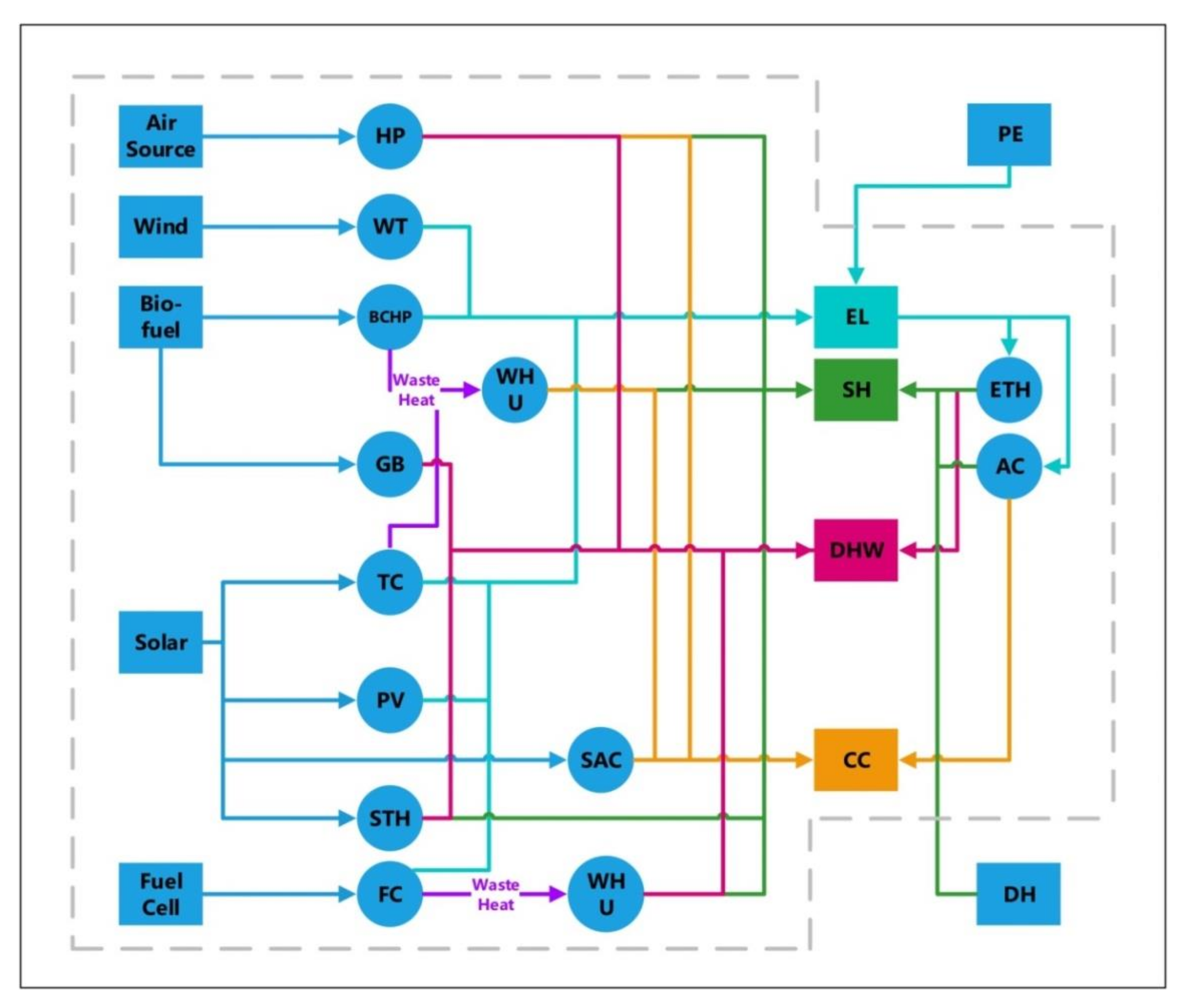
A simple example of MENR system is presented in Figure 1 and only some essential elements are mentioned. For the complex MENR systems, more elements should be considered, such as solar PV system with electric vehicles and energy provided by energy storage systems.
An MENR system should be capable of reducing the power loss, extending the investment horizon of the power network and improving the power quality. Thus, energy quality management (EQM) needs to be investigated in the context of an MENR system [2,3]. EQM is defined as a technique that aims at optimally utilizing the contents of various renewable energy sources, identify inefficiencies in energy systems, and therefore reduce the primary energy consumption [4]. The main tasks of the EQM approach are classified into two steps: energy demand analysis and energy supply system optimization [5]. The energy demand analysis aims to reduce unnecessary energy consumption and provide accurate inputs for energy supply system optimization. Energy supply system optimization focuses on exploring the most suitable system on the basis of renewable energy sources and fulfilling various sustainable requirements, such as high energy performance, low environmental impacts and acceptable system reliability.
A review of the literature shows that EQM is widely used for almost all types and scales of energy systems [6,7]. Guo implemented an EQM approach to undertake multi-objective optimal planning for a stand-alone microgrid (SAMG) system. The goal is to find out the Pareto-optimal solution for the site and capacity of distributed generation in the SAMG as well as the contract price between the distribution company and the distributed generation owner [8]. Dolara applied EQM for a realistic case study microgrid installed in Somalia. The case study introduces an islanded micro-grid supplying the city of Garowe by means of a hybrid power plant of diesel generators, photovoltaic systems and batteries. The EQM process is based on precise analyses of load demand and renewable energy production [9]. Instead, there are only few references for optimizing a MENR system in the literature.
For the evaluation and optimization of a MENR system, energy performance needs to be included and analyzed in terms of both quantity and quality. Currently, quality of energy, or its so-called exergy, had received more attention in recent decades. Exergy is the measure of the maximum useful work that can be done by a system interacting with a reference environment at a constant pressure P0 and a constant ambient temperature T0 [5]. Exergy efficiency has been proven as one of the most important unambiguous thermodynamic tools to evaluate energy performance of energy systems [10,11]. Therefore, exergy efficiency is selected as the energy performance indicator. From the scope of EQM, space heating (SH), domestic hot water (DHW) and cooling (CC) are regarded as low-exergy energy demands and electricity (EL) is a high-exergy energy supply approach. If high-exergy energy supply technologies are used for satisfying low-exergy energy demand, issue called as “exergy mismatch” will be occurred [7]. It is rather important to avoid exergy mismatch for optimization of MENR system.
Besides, a MENR system also needs to keep the acceptable economic sustainability and system reliability. Hence, life-cycle cost (LCC), which usually refers to the estimation of the economic cost of a product during its life span, is selected as the economic indicator for the MENR system [12,13]. The availability of renewable energy sources, especially concerning wind and solar options, is unpredictable and highly depends on climatic conditions, and energy generated from solar and wind is difficult to balance with real time energy demand [14]. Therefore, the present study hypothesizes implements system reliability in the optimization of a MENR system. The maximum allowable level of loss of power supply probability (LPSP) has been widely applied as system reliability indicator in hybrid energy system optimization [14], wherefore it is applied in the present study.
The subsequent part is dedicated to implementing the proposed EQM approach in a realistic MENR system design for a TA located in Dali, China. Three possible reference MENR system scenarios are presented by estimating their exergy efficiency and life-cycle costs. Then, advanced MENR system scenarios which apply the maximum allowable LPSP values as system constraints are analyzed. The final work for the paper is to investigate the MENR system scenario variations caused by the changing ESS parameters and the scale of electric vehicles (EVs). The results show that MENR scenarios are modified significantly depending on the increasing number of EVs and reducing investment of ESSs.
2. Methodology
2.1. Optimization Algorithm: Genetic Algorithm (GA)
As mentioned in Section 1, one of the main tasks for applications of EQM is the optimization of energy supply system. Here, planning and optimization of an MENR system is an extremely complex process because various decision objectives, constraints and a large number of decision variables are included. The optimization process requires exploring the appropriate solution from a very large number of design alternatives/options, thus the selected algorithm needs to be time-effective. Therefore, a multi-objective optimization approach based on genetic algorithm (GA) is proposed.
GA was introduced by Holland in 1970s and has been applied to a diverse range of scientific and economic problems [15]. It is an efficient method to optimize the sizing of hybrid systems, especially in complex systems, where a large number of parameters have to be considered [16,17]. In last decade, GA had been widely applied to optimize and evaluate energy system for different practical objectives. Bilal utilized GA to design hybrid solar-wind-battery systems that can achieve the customers’ required Loss of Power Supply Probability (LPSP) with a minimum annual economic cost [18]. Mohamed introduced a three-phase multi-objective optimization approach (PR_GA_RF) to minimize the environmental impacts (CO2 emission) and economic cost in dwelling building. The study focused on the influence of energy sources and ventilation heat recovery systems [19]. Later, GA began to be introduced for assisting the relatively complicated energy system design. Zidane applied GA for providing an optimal sizing and operation strategy for micro energy grids equipped with renewable and non-renewable based distributed generation and storage [20]. Su applied GA to take a comparative study about solar energy utilization patterns for different types of districts located in China [21].
2.2. Implementation of GA Model
For the optimization process, GA was implemented into MATLAB environment for selecting the optimum MENR system solutions. At the beginning of an optimization run, the model randomly generates a vector of potential decision variables (yi). The first set of potential combinations is called the initial population. All combinations in the initial generation should be ranked by calculating their fitness function values. Subsequently, the following step is to check the optimization stop criterion, i.e., the number of generations [21]. If the criterion is not met, the creation of a new generation starts.
The creation process of new generation contains four steps:
- (1)
- Selection. 15% of combinations with the highest fitness values are kept as offspring.
- (2)
- Crossover. The characteristics of all combinations are mixed in this operator in order to produce offspring. That means the best from different parents can be combined together, and the operator can improve the individuals for the new generation.
- (3)
- Mutation. 15% of the combinations after crossover operator need to experience mutation process. Mutation changes the structure of each combination separately.
- (4)
- Reinsertion. All combinations after selection-crossover-mutation process needs to be re-ranked by re-calculating their fitness function values. 15% of the new combinations with the lowest fitness values will be replaced by the old combinations kept in selection operator.
New generations repeats the whole process until the optimization stop criterion is met. Finally the optimal solution (combination of decision variables) could be achieved.
2.3. Decision Variables
The main mission of the EQM approach is to search for the most appropriate MENR system scenarios that can match actual energy demand and supply by including numerous decision variables with various objectives and constraints. Therefore, the first step is to make decision variable initiation. In this step, it needs to consider the type, range and step of decision variables. All the decision variables in the proposed optimization problem are continuous variables (. Variables (–) aims at optimally designing the equipment sizes for various energy supply technology candidates in MENR system. Selection of “n” depends on the number of available energy conversion systems. The equipment size for each energy supply technology could be calculated by following [4,5]. The corresponding variable constraints are in Equations (1)–(4):
where , , and represent the supply profile of each electricity (EL), space heating (SH), domestic hot water (DHW) and cooling (CC) supply technology, ti is operation time of each energy supply technology. , , and are the total amounts of EL, SH, DHW and CC demand, respectively. , and represent the total amounts of SH, DHW and CC converted from waste heat, respectively.
Besides, variables (–) are considered to represent the sizes of different energy storage systems. Selections of “n + 1” and “n + 3” mean the total capacity of battery and thermal storage (TS), respectively. Selection of “n + 2” represents the power of battery and selection of “n + 4” is the thermal power of TS. Selections “n + 5” and “n + 6” are to optimize the potential size of electric vehicles (EVs) which use vehicle to grid (V2G) technology to support the MENR system as electricity storage systems.
The last three variables (yn+7–yn+9) describe “the ratios of waste heat utilization (WHU)”, indicating the share of waste heat used for satisfying thermal energy demands (SH, DHW and CC demand). The sum of WHU for thermal energy could not exceed the total amount of waste heat. The decision variable vector is expressed as Equation (5):
For the optimization process, potential energy conversion alternatives are: bio-fuel micro-turbine combined power and heat (BCHP) system, fuel cell combined power and heat (FC) system, small scale wind turbine (WT), solar photovoltaic (PV) system, solar PV/thermal (PVT) system, parabolic trough solar power generation (PT) system, solar thermal collector heater (STH), electrical air-conditioner (AC), air source heat pump (HP), biogas boiler (GB), electrical thermal heater (ETH), solar absorption cooling (SAC) system as well as public centralized electricity grid (PE). Also, energy storage alternatives are battery, thermal storage (TS) and EVs with V2G technology (EVV2G). All these energy conversion and storage options has potential to be used for satisfying electricity (EL) demand and thermal energy demands, such as space heating (SH), domestic hot water (DHW) and cooling (CC). Waste heat from electricity generation process is proposed to contribute to providing thermal energy. It should be noticed that the annual energy conversion time of PV and PVT system is 1450 h (3, 4 and 5 h for winter, mid-season and summer day, respectively) and that for PT system is approximately 1600 h (3, 4.5 and 6 h for winter, mid-season and summer day, respectively). STH and SAC systems might operate for 1950 h per year (4, 5 and 7 h for winter, mid-season and summer day, respectively). Annual energy conversion time of wind power technology is set as 1500 h. To promote the system reliability, the bio-energy and fuel cell conversion technologies are assumed to operate for 7000 h per year [21].
Based on these energy conversion systems and coupled with the definition of decision variables, twenty-seven optimization variables are initiated in Table 1.
2.4. Objective Functions
The objective functions entail maximizing the exergy efficiency (EE) of the MENR system and minimizing the life cycle cost (LCC) for providing one unit (kWh) of energy at the boundary of the demand point. The general form of the optimization problem can be expressed as Equation (6):
where and are the EE and LCC of the energy system, respectively. is the vector of continuous decision variables (), as defined in the optimization objective sector.
The first objective function is EE of the entire energy system (), which is calculated from Equation (7) [22]:
where and are the total exergy output and the total exergy input for the MENR system, respectively. In the case of thermal energy, the maximum theoretical exergy content is determined by the Carnot efficiency as . Besides, FQ values for electricity and kinetic energy are set as 1 and 0.91, respectively [4].
The second objective function () is to calculate LCC value of MENR system, covering the cumulative cost throughout its life cycle from the installation to recycling. In the economic model, LCC incorporates five parts: component cost (), installation cost (), replacement cost (), maintenance cost () and recycling cost (), and the objective function f2 is their sum:
The replacement costs are calculated knowing present worth for all components as Equation (9).
where is the replacement cost related to each component in the entire energy system and represent is the present worth factor for an item that will be purchased n years later [23]. The present worth factor for the single payment including inflation is calculated from:
where i represents the inflation rate and d is the discount rate. The average escalation rates of 4.3% and 6.2% for electricity and gas price have been examined [24]. A discount rate of 3% is used in the transition problem. could be calculated using cumulative present worth factor as Equation (11):
where is present worth of maintenance cost and is defined in Equation (10).
After confirmation of optimization objectives, all of these objectives should be compressed as a fitness function shown as Equation (12):
where is the weight of . Here, the weights are set as by the decision makers. is the value of the reference energy system. Number “i” means the number of optimization objectives. For the paper, Number “i” is equal to 2. The weights are assumed as equal importance (), LCC oriented () and EE oriented ().
Besides the objectives, constraints need to be assigned for the optimization process according to the systemic requirements. Here, the reliability of the system is expressed through the LPSP constraint. It is prevented from exceeding the maximum allowable (user-defined) value, which is represented in the model as a constraint function
where Constant is the maximum allowable LPSP value which is predefined by the users.
LPSP is defined as the probability of an insufficient energy supply, i.e., determining the number of hours the MENR system is unable to satisfy the load demand. Inversely, an LPSP value of 0 means the load demand will be always satisfied and the LPSP value of 1 means that the load demand will never be satisfied. It is calculated from Equations (14) and (15) [14]:
where Time is number of hours which require energy demand, and are power of energy supply and energy demand. For MENR system, can be expressed as:
where is the power of each energy conversion system, is the power of energy storage system. For an advanced sustainable energy system, the maximum allowable LPSP value should be less than 10% [14].
3. Case Study
3.1. Brief Information
For the present study, the proposed EQM approach is applied to a TA called Xizhou Town in Dali, China. The target is to find out an optimum MENR system scenario for Xizhou town. Dali is a city in the south of China, located on a fertile plateau between the Cangshan Mountain to the west and Erhai Lake to the east. It is one of the most popular tourist destinations in China, due to both its historic sites and natural beauty. To protect the natural beauty in Xizhou Town, a MENR system is required by the Dali government to replace the existing energy system for providing sustainable and reliable energy.
As a typical TA, the energy utilization pattern of Xizhou Town follows the description introduced in Section 1. To make the optimization process time-effective, representative days for each season are widely applied to point out the optimal designing issues [4,5,21]. The energy demands of this town have been modeled by making use of measured energy consumption data from three representative days for summer, mid-season and winter. Here, the July day represents the maximum energy demands during the cooling season (summer), the October day represents a mid-season energy demands and the January day represents the maximum energy consumption during the heating season (winter) [21]. The detailed information for these representative days is shown in Table 2.
According to the data in Table 2, it is found that energy demands for Xizhou Town are mainly fulfilled by the public electricity grid. EL, SH and CC demands are completely covered by the public electricity grid while a portion of DHW demand met by a solar water tank system. The price of electricity in Xizhou Town is 6.5 c €/kWh, which is set by the Dali government. The peak load of EL demand in winter time is higher than that in mid-season and summer time. The reason is that a large number of EL is used to provide space heating by electric-driven heating devices. During summer time, almost all DHW demand is fulfilled by solar heating system. Therefore, the peak load of DHW from solar in summer day is much higher than that in winter and mid-season days.
3.2. Energy Demand Analysis
As mentioned in Section 1, energy demand analysis is an essential part of EQM and should be completed to provide accurate energy demand inputs for energy supply system optimization.
Xizhou Town is a famous tourist destination, thus it has been perceived in earlier studies that a great portion of electricity is required to provide SH and CC for keeping indoor climate comfort of hotels and supply DHW for washing. Accordingly, energy demand analysis should divide the current energy demands into high-exergy demand (EL) and low-exergy demands (SH, DHW and CC). The new energy demand profiles for Xizhou Town are demonstrated in Table 3.
During the process, the energy conversion efficiency of electricity-driven heating system is set as 0.98 [25].
The new energy demand profiles will be applied as inputs for developing the optimum MENR system scenarios in Xizhou Town.
3.3. Basic MENR System Scenarios
After energy demand analysis, a multi-objective optimization approach based on GA is applied for exploring the most appropriate MENR system. The approach is initiated by following the methodology in Section 2. Basic MENR system scenarios are presented by maximizing EE of the whole system and minimizing their LCC values. LPSP value is pre-defined as 0. There are three types of basic MENR system scenarios included: LCC and EE are of equal importance (A), LCC oriented (B) and EE oriented (C). The solutions for different representative days (winter, mid-season and summer day) are demonstrated in Table 4.
The detailed information for the MENR system scenarios in Xizhou Town is shown below.
- (1)
- MENR system scenario A: BCHP and WT system are ranked as the top two alternatives for EL supply. The capacities of BCHP and WT system could reach to 12.7 MW and 6.5 MW, respectively. Besides, solar power systems, which include PV and PT technology, begin to participate into the EL generation. The sizes of PV and PT system are 3.1 and 2.6 MW. WHU, STH, HP, GB and SAC technology are the basic elements applied to match thermal energy demands. Except for WHU, STH system plays as the main role for providing thermal energy. The maximum shares of SH and DHW demand fulfilled by STH system are 20.3% and 62.6%, respectively. The size of HP system is optimized as 30.5 MW (15 MW for SH supply, 13.1 MW for DHW supply and 2.4 MW for CC supply). 7.2 MW SAC system is applied to fulfill the CC demand. ESSs are also needed in the scenario. The sizes of battery, TS system and EVV2G are 4.8 MW/19.6 MWh, 22.8 MW/46.2 MWh and 0.4 MW/2.0 MWh.
- (2)
- MENR system scenario B: BCHP system plays as the dominated role for EL generation. Over 61.8% of electricity demand is matched by 21.4 MW BCHP system. Other types of EL supply systems, such as PV and WT system, are almost of equal importance. WHU is the main method for SH supply; more than 75.3% of SH demand is covered by WHU. In the meantime, a major portion of DHW demand is taken charge by STH system. The maximum share might achieve 72.2%. Besides of WHU and STH system, the capacities of other thermal energy supply technologies, which include HP, GB and SAC system, are only 12.9 MW, 4.7 MW and 3.1 MW, respectively. In addition, the optimum sizes of battery, TS system and EVV2G are selected as 1.2 MW/4.4 MWh and 18.4 MW/40.6 MWh and 0.6 MW/2.2 MWh.
- (3)
- MENR system scenario C: EL supply system for the scenario could be divided into three groups. The leading group includes BCHP and WT system, whose capacities are 10.9 and 9.5 MW. The following group contains two types of solar power systems. PV and PT system have nearly the same size (3.7 and 3.8 MW). The final group only has a small scale FC system which is equal to 1.8 MW. Majority of thermal energy demand is fulfilled by HP system. Size of HP system could reach to 55.2 MW (20.2 MW for SH supply, 18.7 MW for DHW supply and 16.3 MW for CC supply). The rest portion of thermal energy demand is provided by WHU coupled with STH, GB and SAC system. Additionally, the sizes of battery, TS system and EVV2G are 7.2 MW/34.6 MWh, 15.8 MW/36.2 MWh and 1.8 MW/5.4 MWh.
3.4. Advanced MENR System Scenarios-System Reliability Analysis
Through the optimization results shown in Section 3.3, it is found that solar and wind power system are widely applied for Xizhou Town. System reliability needs to be carefully considered for wind and solar system design. The maximum allowable LPSP values 1%, 5% and 10% are used in the advanced MENR system scenario analysis. Three groups of advanced (MENR system) scenarios (A1–A3), which correspond to these three values, are presented and compared in Table 5. Here, all the decision objectives have equal importance.
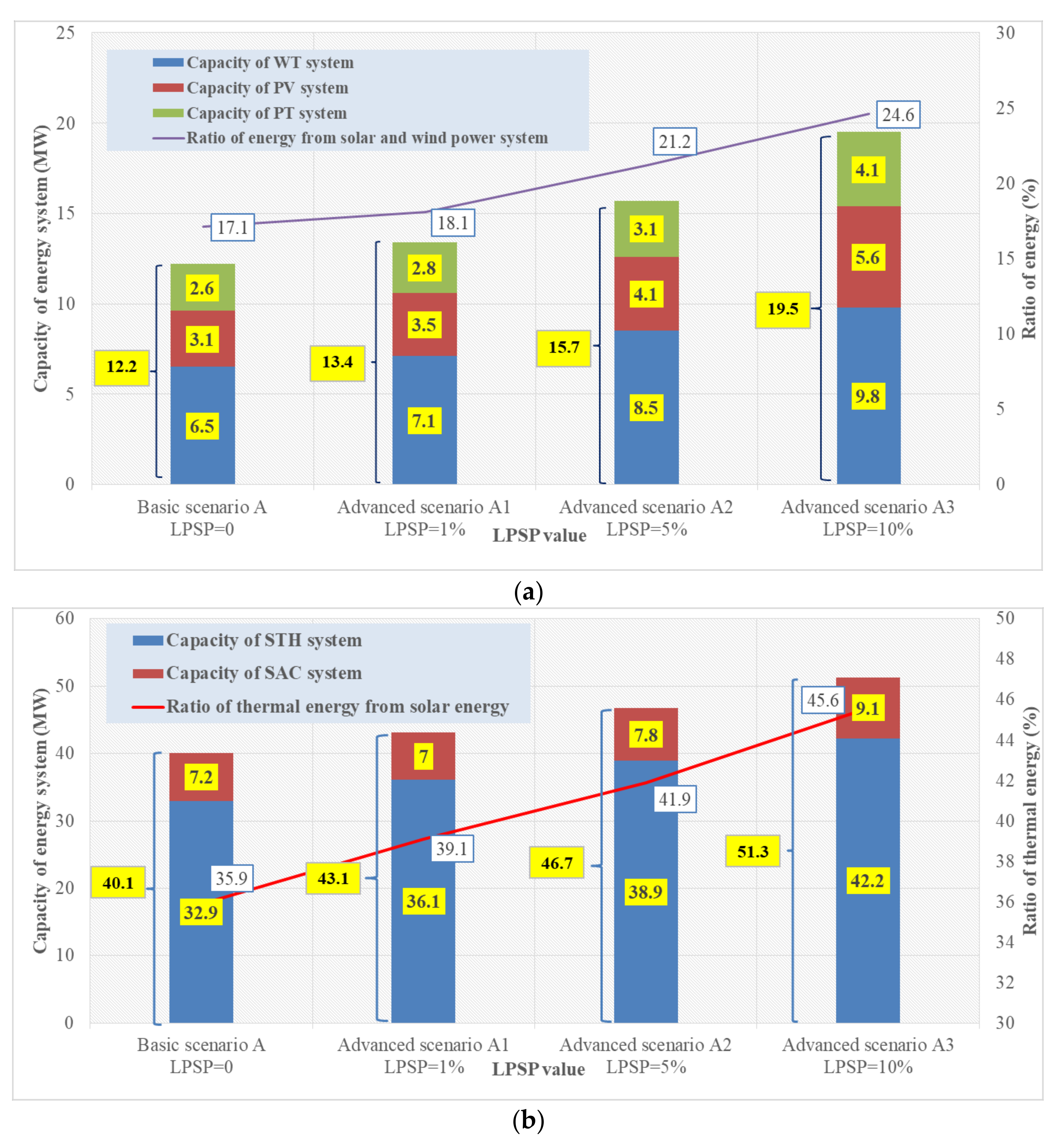
All advanced MENR system scenarios are listed in Table 5. The next step is to make a comparison between basic scenario A and advanced scenarios A1–A3 in Figure 2. Some meaningful information is shown as following.
- (1)
- As the system becomes less reliable (the allowable LPSP values go up from 0% to 10%), an increasing number of energy demands is fulfilled by solar and wind energy shown in Figure 2a. The increment for the total capacity of solar and wind power systems reaches to 60.0% (from 12.2 MW to 19.5 MW). Also, the share of energy demands covered by solar and wind power systems gains 43.9 percent from 17.1% to 24.6%.
- (2)
- Through Figure 2b, it is demonstrated that more and more thermal energy demands are satisfied by solar energy when LPSP value changes from 0% to 10%. The total size of solar thermal energy systems (STH and SAC system) rises more than 27.9 percent to 51.3 MW. Additionally, the ratio of thermal energy taken by solar source maintains a stable growth, from 35.9% to 45.6%.
- (3)
- Although the total capacity of solar and wind power systems rises more than 60 percent, the increment for the size of electricity storage systems (battery and EVV2G) is only 25% according to Figure 2c,d. The main contributor to the increment is the growing size of EVV2G. The size of EVV2G increases from 0.4 MW/2.0 MWh to 2.2 MW/9.2 MWh. As LPSP value decreases, EVV2G might be an electricity storage technology rival for the battery.
- (4)
- When a stable growth (over 27 percent) took place on the size of solar thermal energy systems (STH and SAC system), the size of TS system almost does not increase since LPSP value rises from 0% to 10%, but decreases as LPSP value of 1%. The size of TS system only varies from 22.8 MW/46.2 MWh to 23.8 MW/49.6 MWh. The increments in the capacity and thermal power of TS system are 7.4% and 4.4%, respectively.
Overall, the uncontrollable energy sources, which include solar and wind energy, might contribute more to energy generation (from 52.3 MW to 70.8 MW) since the pre-defined LPSP value increases. Meanwhile, there is just little increase in the total size of ESSs, which rises from 28.0 MW/67.8 MWh to 30.6 MW/76.6 MWh.
From the advanced MENR system scenarios, it is known that the shares of solar and wind energy supply systems are sensitive to the system reliability constraint. Here, ascent of LPSP value means the requirement of system reliability is assumed to decline. Since the maximum allowable LPSP value goes up, solar and wind energy is required to contribute more to energy generation by the support and supplement of ESSs.
4. Parametric Analyses
To protect the environment of Xizhou Town, one of the main tasks required by Dali government is to maximize the penetration of renewable energy sources, such as solar and wind energy. Therefore, it is relevant to consider the research questions like “How the solar energy utilization patterns will change with reducing investments of ESS?” To answer such a question, a parametric study is necessary to show the effects of varying parameters on the basic reference MENR system scenario A for Xizhou Town. Three types of parameters are considered in Section 4.1, Section 4.2 and Section 4.3.
4.1. Investment of Electricity Storage System
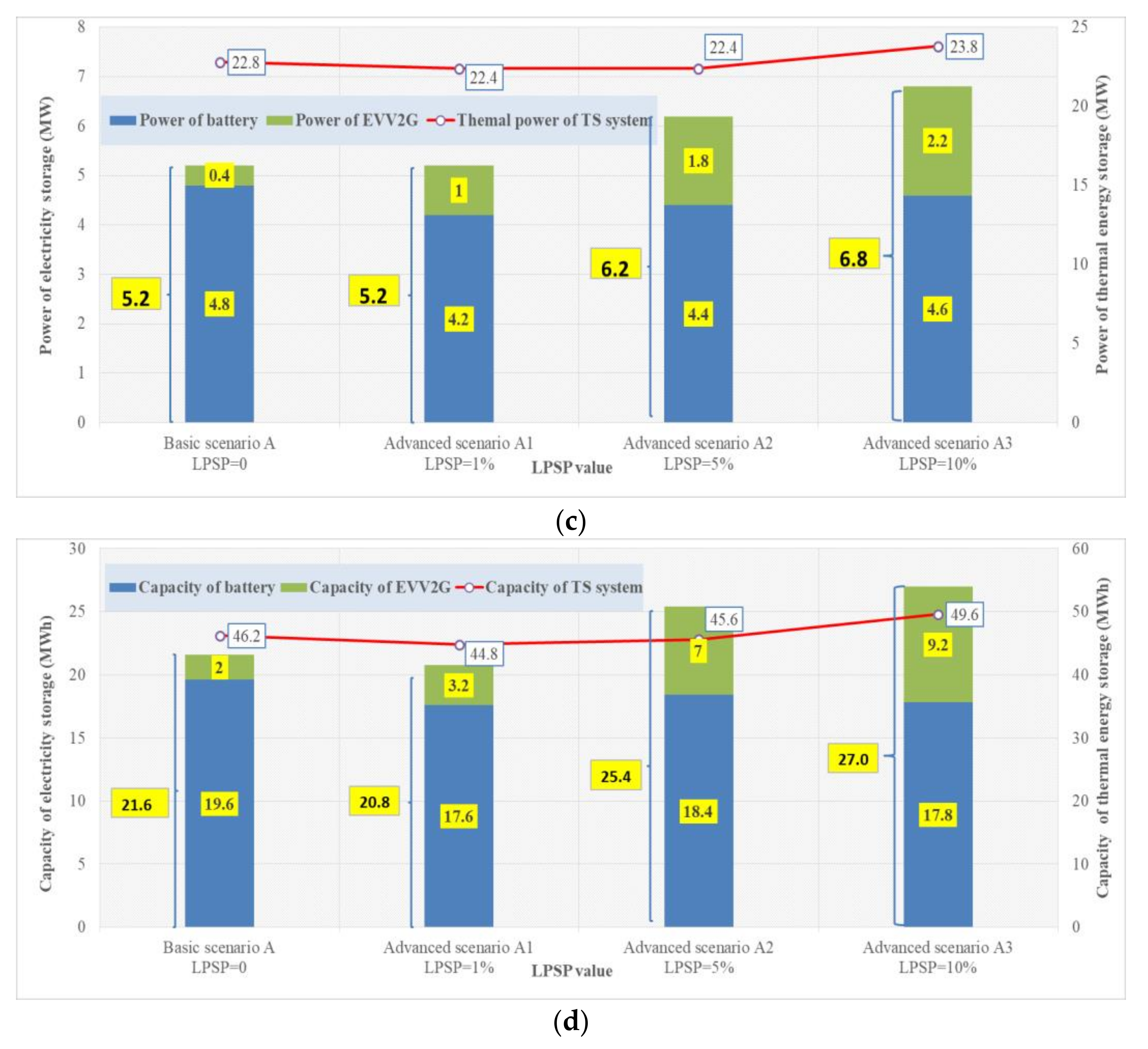
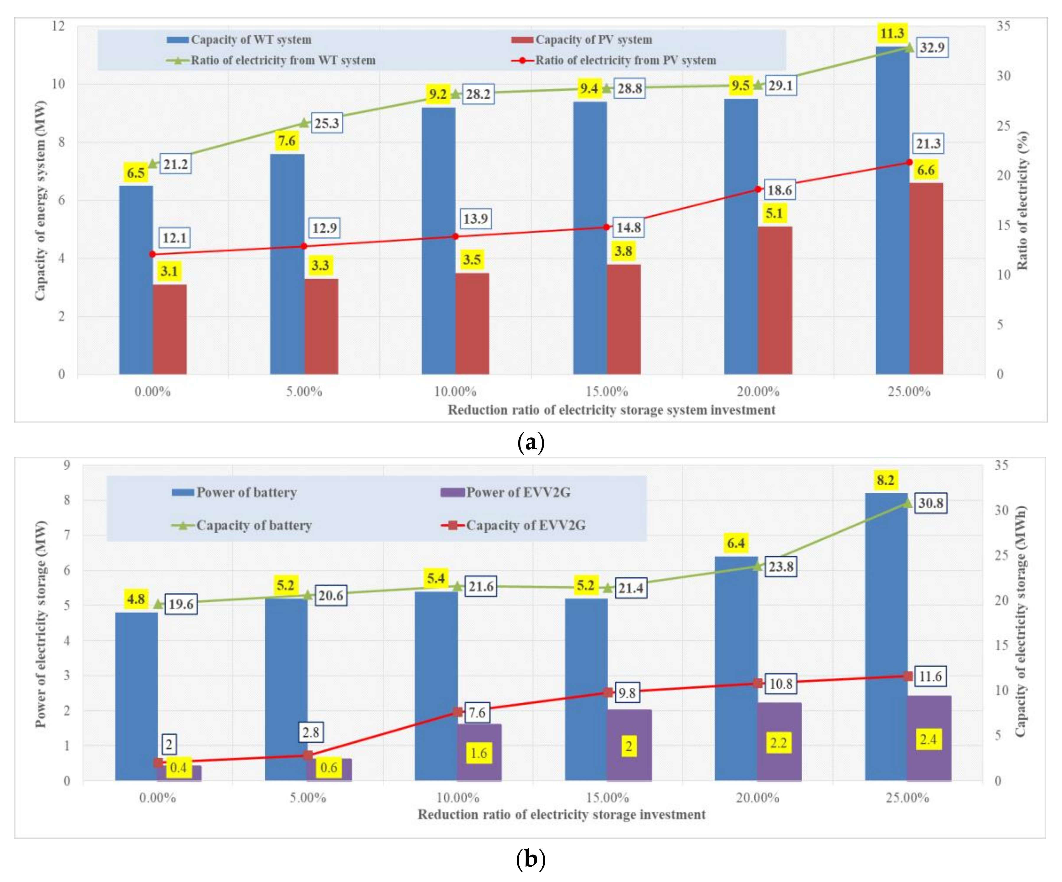
In this part, the investment costs of electricity storage systems are assumed to be decreasing at a certain rate (5–25%), which is predefined as a constraint in the optimization model. Here, life time of MENR system is assumed as 25 years while that of electricity storage system is set as 10 years. The investment reduction is caused by the development of electricity storage technology. The analyzed results related to the MENR system scenario A are shown in Figure 3.
As shown in Figure 3, the trend of basic scenario A is explained as below:
- (1)
- As shown in Figure 3a, it is found that WT and PV system maintain a sustained rise when the investments of electricity storage systems decrease from current level to 75% of current level. There are two ascents for WT system. The first stage is the capacity of WT system rises 41.5 percent from 6.5 MW to 9.2 MW since the reduction ratio increases from 0% to 10%. Then, the share of electricity supplied by WT system varies from 29.1% to 32.9% during the second period. The significant ascent for PV system appears when the reduction ratio increases from 15% to 25%. The increment for the capacity of PV system could reach to 73.7% (from 3.8 MW to 6.6 MW).
- (2)
- The data in Figure 3b shows that the total size of electricity storage systems raises from 5.2 MW/21.6 MWh to 12.6 MW/42.4 MWh. The growth trends for different electricity storage systems, which include battery and EVV2G, are not similar. The sharp ascent for battery happens when the reduction ratio is 15%. The increments for the power and capacity of battery are 57.7% and 43.9%, respectively. For EVV2G, there is a stable and gradual growth since the reduction ratio ascends from 5% to 25%. The size of EVV2G climbs from 0.6 MW/2.8 MWh to 2.4 MW/11.6 MWh.
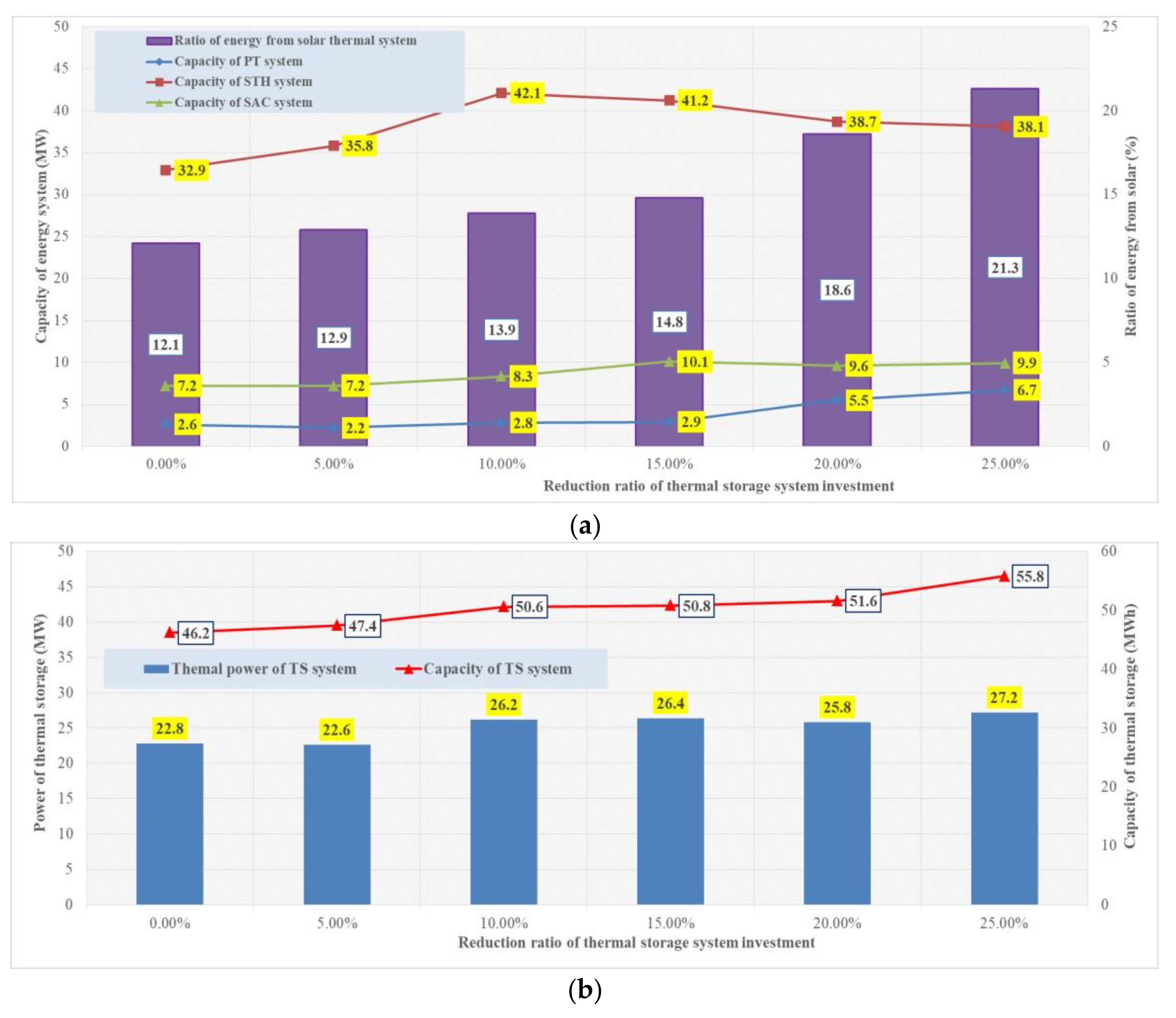
4.2. Investment of TS System
Investment of TS system is assumed to be decreasing at a certain rate predefined as a constraint (5–25%). Here, life time of MENR system is assumed as 25 years while that of TS system is set as 15 years. The analyzed results related to the Xizhou Town are shown in Figure 4.
Through Figure 4, it is found that the total ratio of energy demand fulfilled by solar thermal energy system (PT, STH and SAC system) shows a steady upward trend from 12.1% to 21.3%. The growth trends for different energy supply systems are completely distinct.
- (1)
- The capacity of PT system experiences three periods shown in Figure 4a. It begins at 2.6 MW, and then it goes down to 2.2 MW as reduction ratio is 5%. Subsequently, it climbs slowly to 2.9 MW. Since the reduction ratio reaches to 15%, an upsurge which jumps to 6.7 MW is occurred.
- (2)
- The capacities of STH and SAC system show the same developing trend according to Figure 4a. Both of them go up to the summit and then start to decline. The peak value for the capacity of STH system is 42.1 MW when the reduction ratio is 10%. Accordingly, the summit for the capacity of SAC system is 10.1 MW as the reduction ratio stays at 15%.
- (3)
- Figure 4b presents that the size of TS system maintains a gradual growth, from 22.8 MW/46.2 MWh to 27.2 MW/55.8 MWh. It needs to be noticed that the capacity of TS system decrease from 26.4 MWh to 25.8 MWh when the reduction ratio ascends from 15% to 20%.
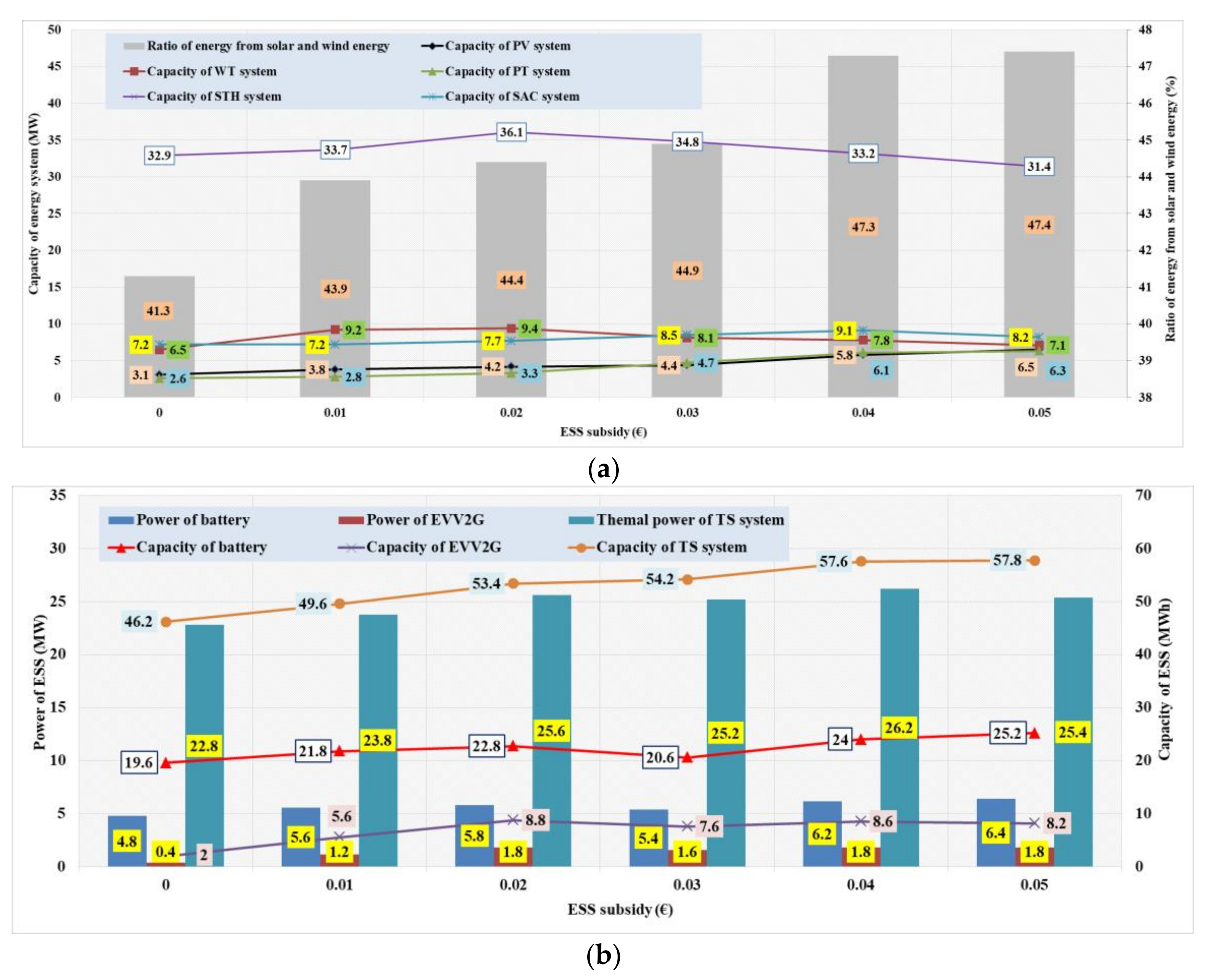
4.3. Energy Storage Subsidy
If the technology development could not reduce the investments of ESSs, it is important to find another way for making the ESS cost-effective. An energy storage subsidy provided by the government is considered as a promising solution. In this part, energy policy parameter “Energy storage subsidy (ESTS)” is assumed to be predefined as constraints, which are subsidies of 0.01 €, 0.02 €, 0.03 €, 0.04 € and 0.05 € for one unit (per kWh) of energy provided by ESSs. The analyzed results related to the MENR system scenario A are shown in Figure 5.
According to Figure 5, it is found that the total ratio of energy provided by solar and wind energy keeps a sustainable growth from 41.3% to 47.4%. The (variation) tendencies for different energy supply systems are various.
- (1)
- Through Figure 5a, development trend for the capacities of WT, STH and SAC system could be expressed as an ascent to summit coupled with a descent. The capacity of WT system goes up to 9.4 MW when ES is 0.03 €, and then it declines to 7.1 MW gradually. Besides, the summits for the capacities of STH and SAC system are 36.1 MW with ESTS of 0.02 € and 9.1 MW with ESTS of 0.04 €, respectively. The other two energy supply systems (PV and PT system) maintain a steady rise. The increments for the capacities of PV and PT system are 3.4 MW and 3.7 MW, respectively. When ESTS reaches to 0.05 €, it is found that PV, PT and WT system have nearly the identical sizes, which are 6.5 MW, 6.3 MW and 7.1 MW.
- (2)
- According to Figure 5b, it is presented that the size of battery climbs from 4.8 MW/19.6 MWh to 6.4 MW/25.2 MWh smoothly. The size of EVV2G jumps from 0.4 MW/2 MWh to 1.2 MW/5.6 MWh when ESTS rises from 0 to 0.01 €, and then increase to 1.8 MW/8.8 MWh as ESTS of 0.02 €. Although the ESTS continues to grow, there is little change happens on the size of EVV2G. The final size of EVV2G is 1.8 MW/8.2 MWh. The size of TS system keeps growing with the ups and downs. Power of TS system goes up to 25.6 MW when ES is 0.02 €, and then it decrease to 25.2 MW. Finally, it could rebound to 26.2 MW. Accordingly, the capacity of TS system shows an upward trend, which is from 46.2 MWh to 57.8 MWh.
4.4. Insights and Implications
Through the parametric study in Section 4.1, Section 4.2 and Section 4.3, some useful information could be found to guide the integration of renewable energy systems and ESSs.
- (1)
- The main bottleneck of the implementation of electricity storage systems is summarized as its high expense. No matter investment reduction or energy storage subsidy provided by government; the essence of these methods is to make electricity storage systems cost-effective. When the economic cost of electricity storage system stays at an acceptable level, electricity storage technology might goes into booming.
- (2)
- Thermal energy storage technology has been widely applied for the town. Currently, the main purpose of TS system is to hold low- and medium-temperature thermal energy. As the economic cost of TS system reaches to an acceptable level, TS system might be utilized in some high-temperature context, such as high-temperature solar energy application.
- (3)
- Renewable energy systems, especially solar and wind energy systems are influenced by energy sources because of the intermittent solar radiation and wind speed characteristics. To maintain system reliability, solar and wind energy system need to be coupled with ESSs. With the economic cost reduction of ESSs, solar power generation systems will play more and more important role for energy generation.
5. EVs Analysis
5.1. Load Profile with Increasing Scale of EVs
Dali government plans to put 200 to 400 EVs in Xizhou Town for public transportation in order to reduce the number of traditional fuel vehicles. 260 EV charge piles have been established in Xizhou Town. The detailed information is presented in Table 6.
The charging time of EVs is divided into two periods: 11:00–14:00 and 23:00–7:00 (next day). Due to the charging time regulation and the status of EV charging facilities, the coordinated charging strategies for different numbers of EVs might be completely distinct. Three types of coordinated charging strategies for 200, 300 and 400 EVs are listed in Table 7.
The increasing scale of EVs utilized in Xizhou Town will change the electricity demands and profiles presented in Table 3. The new electricity utilization pattern is demonstrated in Table 8.
According to these new electricity demand profiles, it is found that peak load of electricity demand keeps a stable rise. The values for winter, summer and mid-season reach to 35.4 MW, 30.99 MW and 32.4 MW when 400 EVs are applied in the town. Although the differences between peak and valley load are aggravated in all seasons, the times for valley loads are shifted. Currently, the valley load without EVs in mid-season is 4.4 MW appeared in 5:00 (shown in Table 3b). When the number of EVs reaches to 400, the valley load is modified as 5.38 MW in 15:00.
5.2. Effects on MENR Scenario with Increasing Scale of EVs
The new electricity profiles might influence the selection of optimal MENR system scenarios. In this part, three types of MENR system scenarios (AA1–AA3) are optimized for different scales of EVs. The EL demand is presented in Table 8 and the thermal energy demands (SH, DHW and CC) are from Table 3. Here, all the decision objectives have equal importance and the maximum allowable LPSP value is 0. All the optimization results are demonstrated in Table 9.
According to Table 9, some meaningful information is shown as follows:
- (1)
- Solar and wind power systems are playing more and more important roles for energy supply. The capacities of WT, PV and PT system rise from 8.1 MW, 3.9 MW and 3.6 MW to 11.5 MW, 6.5 MW and 5.2 MW, respectively. The explanation for the phenomena is that the output characteristics of solar and wind power systems are suitable for matching the increasing EL demand caused by the growth of EVs. The extra EL demand appears as two periods, which are 11:00–14:00 and 0:00–6:00. Solar power systems, such as PV and PT system, have potential to fulfill the additional EL demand during 11:00–14:00. Conversely, WT system could take charge for the extra EL demand happens from 0:00 to 6:00.
- (2)
- Increasing penetration of solar and wind energy might leads to the growth of ESSs. The total size of electricity storage systems raises from 7.0 MW/27.8 MWh to 9.2 MW/34.2 MWh. Such increase is applied to support the ascents of WT and PV system. It is found that battery does not have dominated position for electricity storage. As the number of EVs increase to 300, the size of battery (4.4 MW/14.4 MWh) is smaller than that of EVV2G (4.8 MW/19.8 MWh). Meanwhile, the size of TS system also goes up from 21.7 MW/45.4 MWh to 23.2 MW/58.4 MWh. The increment is an effective supplement for PT system.
5.3. Insights and Implications
According to the EVs analyses in Section 5.1 and Section 5.2, some useful guidance could be found to support the development of EVs.
- (1)
- Increasing scale of EVs might change the energy demand profiles completely. As the government encourages using EVs by making policies, optimal designing of MENR system should consider the number of EVs. The share of solar and wind energy system presents an upward growth tendency while the number of EVs keeps increasing.
- (2)
- It is important to apply EQM approach to arrange the charging strategy for EVs. Without the EQM method, the charging strategy might lead to aggravating the difference between peak and valley load.
- (3)
- Large scale of EVs could be regarded as a number of movable battery modules. With assistance of V2G technology, EVs could be applied for providing electricity. In future, EVs with V2G technology might be the main force of electricity storage.
6. Conclusions
Although EQM had been widely accepted in many scientific technical fields, the main novelty of the paper could be summarized as application of EQM for a specific type of area. Also, some new elements, such as EVs connected with grid, are considered for the EQM process. Here, a multi-objective energy quality management approach based on genetic algorithm (GA) is proposed and applied to search for the optimal MENR system scenarios for a tourist area (TA) called Xizhou Town located in Dali, China. The basic scenarios are selected as the optimal hybrid energy systems with maximum exergy efficiency and minimum life-cycle costs (LCC). There are three types of basic MENR system scenarios included: LCC and EE are of equal importance, LCC oriented and EE oriented. Then, advanced MENR scenarios coupled with system reliability are discussed. The loss of power supply probability (LPSP) is predefined as system reliability indicator. The maximum allowable level of LPSP value is no more than 10%. Finally, the study investigates the effects of various ESSs parameters and the number of EVs on selected MENR scenarios. Some useful conclusions about the MENR scenarios can be drawn:
- (1)
- Thermal storage (TS) system and electricity storage system are two major types of ESSs. TS system has lower investment than electricity storage system, such as battery and EVV2G. Currently, TS system has been widely applied for providing reliable thermal energy to users and electricity generation. Therefore, investment reduction hardly influences the utilization status of TS system.
- (2)
- Utilization status of solar and wind energy supply systems is sensitive.to the system reliability constraint. Here, LPSP value is selected as system reliability indicator. Ascent of LPSP value means the requirement of system reliability is assumed to decline. Since the pre-defined LPSP value increases, solar and wind energy might contribute more to energy generation. Meanwhile, there is little improvement for the total size of ESSs.
- (3)
- It needs to be noticed that all solar and wind power systems might have almost identical capacities when the subsidy for ESS reaches to a certain level. For the case study in Xizhou town, the certain level is optimized as 0.05 € per unit (kWh). The optimized ESS subsidy value would vary with different cases.
- (4)
- Increasing scale of EVs might aggravate the difference between peak and valley load. Two solutions are required to face such deterioration. Firstly, charging strategies for EVs needs to be optimally arranged by introducing EQM approach. Secondly, more ESSs are required. As the number of EVs increases from 0 to 400, the required size of ESS shows a significant ascent. The total size of electricity storage systems raises from 7.0 MW/27.8 MWh to 9.2 MW/34.2 MWh. Meanwhile, the size of TS system also goes up from 21.7 MW/45.4 MWh to 23.2 MW/58.4 MWh. In addition, solar and wind power systems are playing more and more important roles for energy generation. The reason could be briefly summarized as that the output characteristics of solar and wind power systems are suitable for satisfying the extra EL demand caused by the increasing scale of EVs.
For the paper, it should be highlighted that the proposed EQM approach concentrates on the initial planning stage and the optimization results are meaningful for planers and policy makers. Therefore, the limitation of this EQM approach is that it only applies steady-state models. Future work will focus on updating the approach. The updated version of EQM approach could be applied for both plan and operation. Therefore, the updated EQM approach needs to include not only steady-sated models but also dynamic models.
Acknowledgments
This work was supported by the Yunnan Power Grid under Grant No. K-YN2014-179.
Author Contributions
Hai Lu and Jiaquan Yang developed energy quality management approach in this paper and wrote this paper. Kari Alanne made some significant improvements for the approach and imporved the language quality of this paper. Li Guo contributed to the EV part and analyze the impacts of EVs.
Conflicts of Interest
The authors declare no conflict of interest.
Nomenclature
| cost, c €/kWh | |
| cost of component, c €/kWh | |
| CO2 equivalent of component, g/kWh | |
| CO2 equivalent of installation, g/kWh | |
| CO2 equivalent of operation, g/kWh | |
| CO2 equivalent of maintenance, g/kWh | |
| CO2 equivalent of recycling, g/kWh | |
| d | discount rate |
| energy, MJ | |
| exergy, MJ | |
| Carnot Factor | |
| i | inflation rate |
| LPSP | loss of power supply probability |
| time of energy required, s | |
| P | power, kW |
| present worth factor | |
| present worth, c €/kWh | |
| Q | energy demand, MJ |
| thermal source temperature, K | |
| constant ambient temperature, K | |
| weight of benefit | |
| Subscripts | |
| CC | cooling capacity demand |
| DHW | domestic hot water demand |
| EL | electricity demand |
| ele | Electricity |
| SH | space heating demand |
| heat | thermal energy |
| in | Input |
| int | Installation |
| man | maintenance |
| out | output |
| recy | recycling |
| rep | replacement |
| waste-SH | waste heat used for space heating |
| waste-DHW | waste heat used for domestic hot water |
| waste-CC | waste heat used for cooling capacity |
| Abbreviations | |
| AC | air conditioner |
| ACCP | alternating current charging pile |
| ACFCP | alternating current fast charging pile |
| BCHP | bio-fuel micro-turbine power and heat |
| CC | cooling capacity |
| CD | commercial district |
| DCFCP | direct current fast charging pile |
| DHW | domestic hot water |
| ESTS | Energy storage subsidy |
| EE | exergy efficiency |
| EQM | energy quality management |
| ESS | energy storage system |
| EV | electric vehicle |
| ESTS | energy storage subsidy |
| EVV2G | electric vehicle with vehicle to grid technology |
| EL | electricity |
| GA | genetic algorithm |
| GB | biogas boiler |
| HP | air source heat pump |
| LCC | life cycle cost |
| LCCO2 | life cycle CO2 equivalent |
| LPSP | loss of power supply probability |
| MENR | micro energy network integrated with renewables |
| PE | public electricity grid |
| PT | parabolic trough solar power generation |
| PV | solar photovoltaic |
| PVT | solar photovoltaic/thermal |
| SAC | solar absorption cooling |
| SAMG | stand-alone microgrid |
| SH | space heating |
| STH | solar thermal heater |
| TA | tourist area |
| TS | thermal storage |
| V2G | vehicle to grid technology |
| WHU | waste heat utilization |
| WT | wind turbine |
References
- Zhao, B.; Zhang, X.; Li, P.; Wang, K.; Xue, M.; Wang, C. Optimal sizing, operatingstrategy and operational experience of a stand-alone microgrid on Dongfushan Island. Appl. Energy 2014, 113, 1656–1666. [Google Scholar] [CrossRef]
- Popov, A.; Popov, M.; Villacci, D.; Terzija, V. An integrated framework for smart microgrids modeling, communication, and verification. Proc. IEEE 2011, 99, 119–132. [Google Scholar]
- Khodaei, A. Microgrid optimal scheduling with multi-period islanding constraints. IEEE Trans. Power Syst. 2014, 29, 1383–1392. [Google Scholar] [CrossRef]
- Lu, H.; Alanne, K.; Martinac, I. Energy quality management for building clusters and districts (BCDs) through multi-objective optimization. Energy Convers. Manag. 2014, 79, 525–533. [Google Scholar] [CrossRef]
- Lu, H. Energy Quality Management for Building Clusters/Districts. Licentiate Thesis, Royal Institute of Technology, Stockholm, Sweden, 2013. [Google Scholar]
- Lin, W.; Tu, C.; Tsai, M. Energy Management Strategy for Microgrids by Using Enhanced Bee Colony Optimization. Energies 2016, 9, 5. [Google Scholar] [CrossRef]
- Kilkiş, Ş. A rational exergy management model for curbing building CO2 emission. ASHRAE 2005, 113, 113–123. [Google Scholar]
- Guo, L.; Wang, N.; Lu, H. Multi-objective optimal planning of the stand-alone microgrid system based on different benefit subjects. Energy 2016, 116, 353–363. [Google Scholar] [CrossRef]
- Dolara, A.; Grimaccia, F.; Magistrati, G.; Marchegiani, G. Optimization Models for Islanded Micro-Grids: A Comparative Analysis between Linear Programming and Mixed Integer Programming. Energies 2017, 10, 241. [Google Scholar] [CrossRef]
- Szargut, J.; Morris, D.R.; Stewart, F.R. Exergy Analysis of Thermal, Chemical, and Metallurgical Processes; Edwards Brothers Inc.: Ann Arbor, MI, USA, 1998. [Google Scholar]
- Rosen, M.A.; Dincer, I. Exergy methods for assessing and comparing thermal storage systems. Int. J. Energy Res. 2003, 27, 415–430. [Google Scholar] [CrossRef]
- Crawford, R.H. Life cycle energy and greenhouse emissions analysis of wind turbines and the effect of size on energy yield. Renew. Sustain. Energy Rev. 2009, 13, 2653–2660. [Google Scholar] [CrossRef]
- Sherwani, A.F.; Usmani, J.A. Varun, Life cycle assessment of solar PV based electricity generation systems: A review. Renew. Sustain. Energy Rev. 2010, 14, 540–544. [Google Scholar] [CrossRef]
- Yang, H.; Zhou, W.; Liu, L. Optimal sizing method for stand-alone hybrid solar-wind system with LPSP technology by using genetic algorithm. Sol. Energy 2008, 82, 354–367. [Google Scholar] [CrossRef]
- Congradac, V.; Kulic, F. HVAC system optimization with CO2 concentration control using genetic algorithms. Energy Build. 2009, 41, 571–577. [Google Scholar] [CrossRef]
- Holland, J.H. Adaptation in Natural and Artificial Systems; The University of Michigan Press: Ann Arbor, MI, USA, 1975. [Google Scholar]
- Erdinc, O.; Uzunoglu, M. Optimum design of hybrid renewable energy systems: Overview of different approaches. Renew. Sustain. Energy Rev. 2012, 16, 1412–1425. [Google Scholar] [CrossRef]
- Ould Bilal, B.; Sambou, V.; Ndiaye, P.A.; Kébé, C.M.F.; Ndongo, M. Optimal design of a hybrid solar-wind-battery system using the minimization of the annualized cost system and the minimization of the loss of power supply probalility (LPSP). Renew. Energy 2010, 35, 2388–2390. [Google Scholar] [CrossRef]
- Mohamed, H.; Ala, H.; Kai, S. Applying a multi-objective optimization approach for design of low-emission cost-effective dwellings. Build. Environ. 2011, 46, 109–123. [Google Scholar]
- Zidan, A.; Gabbar, H.A. DG Mix and Energy Storage Units for Optimal Planning of Self-Sufficient Micro Energy Grids. Energies 2016, 9, 616. [Google Scholar] [CrossRef]
- Su, S.; Lu, H.; Zhang, L.; Alanne, K.; Yu, Z. Solar energy utilization patterns for different district typologies using multi-objective optimization: A comparative study in China. Sol. Energy 2017, 155, 246–258. [Google Scholar] [CrossRef]
- Abbes, D.; Martinez, A.; Champonois, G. Life cycle cost, embodied energy and loss of power supply probability for the optimal design of hybrid power systems. Math. Comput. Simul. 2014, 98, 46–62. [Google Scholar] [CrossRef]
- Lu, H.; Yu, Z.; Alanne, K.; Xu, X.; Fan, L.; Yu, H.; Zhang, L.; Martinac, I. Parametric analysis of energy quality management for district in China using multi-objective optimization approach. Energy Convers. Manag. 2014, 87, 636–646. [Google Scholar] [CrossRef]
- Lam, J.C.; Chan, W.W. Life cycle energy cost analysis of heat pump application for hotel swiming pools. Energy Convers. Manag. 2001, 42, 1299–1306. [Google Scholar] [CrossRef]
- Henning, H.M.; Palzer, A. A comprehensive model for the German electricity and heat sector in a future energy system with a dominant contribution from renewable energy technologies—Part I: Methodology. Renew. Sustain. Energy Rev. 2014, 30, 1003–1018. [Google Scholar] [CrossRef]
Figure 1.
Example of MENR system. A demonstration of ideal MENR system.

Figure 2.
Change of MENR system with different LPSP values in Xizhou Town. Changes of MENR system with different LPSP values in Xizhou Town. (a) Change of solar and wind power system; (b) Change of solar thermal energy system; (c) Change for power of energy storage system; (d) Change for capacity of energy storage system.


Figure 3.
Parametric study for investment reduction of electricity storage system. Variations on solar/wind power system and ESSs with reducing investment of electricity storage system. (a) Size variation of WT and PV system; (b) Size variation of electricity storage system.
Figure 3.
Parametric study for investment reduction of electricity storage system. Variations on solar/wind power system and ESSs with reducing investment of electricity storage system. (a) Size variation of WT and PV system; (b) Size variation of electricity storage system.

Figure 4.
Parametric study for investment reduction of TS system. Variations on solar thermal energy system and TS systems with reducing investment of TS system. (a) Size variation of solar thermal energy system; (b) Size variation of TS system.
Figure 4.
Parametric study for investment reduction of TS system. Variations on solar thermal energy system and TS systems with reducing investment of TS system. (a) Size variation of solar thermal energy system; (b) Size variation of TS system.

Figure 5.
Parametric study for ESS subsidy. Variations on solar/wind energy system and ESSs with increasing subsidy for ESS. (a) Size variation of solar and wind energy system; (b) Size variation of ESS.
Figure 5.
Parametric study for ESS subsidy. Variations on solar/wind energy system and ESSs with increasing subsidy for ESS. (a) Size variation of solar and wind energy system; (b) Size variation of ESS.


Table 1.
Optimization variables instantiation.
| Variables | y | Variable Type | Range of Value | Step |
|---|---|---|---|---|
| Ratio of BCHP | y1 | Continuous | [0, 100%] | 0.1% |
| Ratio of WT | y2 | Continuous | [0, 100%] | 0.1% |
| Ratio of PV | y3 | Continuous | [0, 100%] | 0.1% |
| Ratio of PVT | y4 | Continuous | [0, 100%] | 0.1% |
| Ratio of PT | y5 | Continuous | [0, 100%] | 0.1% |
| Ratio of PE | y6 | Continuous | [0, 100%] | 0.1% |
| Ratio of FC | y7 | Continuous | [0, 100%] | 0.1% |
| Ratio of HP for SH | y8 | Continuous | [0, 100%] | 0.1% |
| Ratio of STH for SH | y9 | Continuous | [0, 100%] | 0.1% |
| Ratio of AC for SH | y10 | Continuous | [0, 100%] | 0.1% |
| Ratio of ETH for SH | y11 | Continuous | [0, 100%] | 0.1% |
| Ratio of HP for DHW | y12 | Continuous | [0, 100%] | 0.1% |
| Ratio of STH for DHW | y13 | Continuous | [0, 100%] | 0.1% |
| Ratio of GB | y14 | Continuous | [0, 100%] | 0.1% |
| Ratio of ETH for DHW | y15 | Continuous | [0, 100%] | 0.1% |
| Ratio of SAC | y16 | Continuous | [0, 100%] | 0.1% |
| Ratio of HP for CC | y17 | Continuous | [0, 100%] | 0.1% |
| Ratio of AC for CC | y18 | Continuous | [0, 100%] | 0.1% |
| Power of battery | y19 | Continuous | [0, PEL-peak] * | 0.1 MW |
| Capacity of battery | y20 | Continuous | [0, QEL] * | 0.1 MWh |
| Thermal power of TS | y21 | Continuous | [0, PH-peak] ** | 0.1 MW |
| Capacity of TS | y22 | Continuous | [0, QH] ** | 0.1 MWh |
| Power of EVV2G | y23 | Continuous | [0, PEL-peak] * | 0.1 MW |
| Capacity of EVV2G | y24 | Continuous | [0, QEL] * | 0.1 MWh |
| Ratio of WHU for SH supply | y25 | Continuous | [0, 100%] | 0.1% |
| Ratio of WHU for DHW supply | y26 | Continuous | [0, 100%] | 0.1% |
| Ratio of WHU for CC supply | y27 | Continuous | [0, 100%] | 0.1% |
* PEL-peak is peak load of electricity demand (MW); QEL is electricity demand (MWh). ** PH-peak is peak load of all thermal energy demand, which includes SH, DHW and CC (MW); QH is thermal energy demand, which includes SH, DHW and CC (MWh).
Table 2.
Energy demands and load profiles for Xizhou town on three representative days.
| Winter Day | Mid-Season Day | Summer Day |  | ||||
| PL * (MW) | EC (MWh/day) | PL (MW) | EC (MWh/day) | PL (MW) | EC (MWh/day) | ||
| EL from grid ** | 99.21 | 1227.11 | 56.8 | 561.33 | 73.89 | 958.48 | |
| DHW from solar ** | 6.98 | 58.63 | 9.12 | 108.36 | 14.79 | 171.38 | |
| * PL-Peak load; EC-Energy consumption. ** The data is provided by Zhejiang University in 2016. | |||||||
Table 3.
New energy demands and load profiles for Xizhou town after energy demand analysis.
| a. New Energy Demands and Load Profile in Typical Winter Day | |||
| Winter Day |  | ||
| PL (MW) | EC (MWh/day) | ||
| EL | 27.4 | 274.63 | |
| SH | 52.8 | 744.12 | |
| DHW | 38.3 | 356.8 | |
| CC | 3.1 | 16.00 | |
| b. New Energy Demands and Load Profile in Typical Mid-Season Day | |||
| Mid-Season Day |  | ||
| PL (MW) | EC (MWh/day) | ||
| EL | 24.4 | 283.36 | |
| SH | 3.2 | 28.22 | |
| DHW | 23.1 | 279.31 | |
| CC | 20.1 | 109.72 | |
| c. New Energy Demands and Load Profile in Typical Summer Day | |||
| Summer Day |  | ||
| PL (MW) | EC (MWh/day) | ||
| EL | 23.0 | 304.18 | |
| DHW | 35.7 | 419.11 | |
| CC | 33.4 | 419.31 | |
Table 4.
Basic optimal MENR system scenarios in Xizhou Town.
| Alternative | A | B | C | ||||||||||
|---|---|---|---|---|---|---|---|---|---|---|---|---|---|
| Size * (MW) | Ratio of Energy Production (%) | Size * (MW) | Ratio of Energy Production (%) | Size * (MW) | Ratio of Energy Production (%) | ||||||||
| W ** | M ** | S ** | W | M | S | W | M | S | |||||
| EL | BCHP | 12.7 | 46.4 | 34.3 | 35.2 | 21.4 | 78.2 | 61.8 | 68.1 | 10.9 | 39.9 | 32.9 | 38.7 |
| WT | 6.5 | 26.7 | 21.2 | 16.2 | 1.6 | 5.8 | 4.7 | 2.1 | 9.5 | 34.4 | 28.4 | 19.6 | |
| PV | 3.1 | 7.4 | 13.2 | 14.4 | 2.6 | 2.5 | 10.7 | 10.8 | 3.8 | 9.1 | 15.5 | 15.8 | |
| PT | 2.6 | 5.1 | 6.6 | 12.2 | 1.2 | 2.3 | 4.9 | 4.8 | 3.7 | 6.7 | 10.9 | 13.4 | |
| FC | 1.2 | 4.2 | 4.1 | 5.6 | - | - | - | - | 1.8 | 5.2 | 7.1 | 7.6 | |
| PE | - | 10.2 | 20.6 | 16.4 | - | 11.2 | 17.9 | 15.2 | - | 4.7 | 5.2 | 4.9 | |
| SH | WHU | - | 51.4 | 100 | - | - | 75.3 | 100 | - | - | 40.8 | 100 | - |
| HP *** | 15.0 | 28.3 | - | - | 4.6 | 8.7 | - | - | 20.2 | 38.3 | - | - | |
| STH | 10.6 | 20.3 | - | - | 8.5 | 16.0 | - | - | 11.0 | 20.9 | - | - | |
| DHW | WHU | - | 12.0 | 10.3 | - | - | 17.6 | 22.2 | - | - | 13.8 | 41.7 | 45.5 |
| STH | 22.3 | 42.4 | 49.9 | 62.6 | 25.8 | 49.7 | 58.3 | 72.2 | 10.2 | 26.5 | 11.0 | 13.7 | |
| HP *** | 13.1 | 34.2 | 29.0 | 23.6 | 8.3 | 21.8 | 19.5 | 14.7 | 18.7 | 48.7 | 28.5 | 32.6 | |
| GB | 4.9 | 11.4 | 10.8 | 13.8 | 4.7 | 10.9 | 17.0 | 13.1 | 4.2 | 11.0 | 8.8 | 7.2 | |
| CC | WHU | - | - | 89.7 | 71.2 | - | - | 100 | 91.5 | - | - | 55.3 | 23.9 |
| HP *** | 2.4 | - | - | 7.2 | - | - | - | - | 16.3 | - | 44.7 | 48.9 | |
| SAC | 7.2 | 100 | 10.3 | 21.6 | 3.1 | 100 | - | 8.5 | 9.1 | 100 | - | 27.2 | |
| Battery (MW/MWh) | 4.8/19.6 | 1.2/4.4 | 7.2/34.6 | ||||||||||
| TS (MW/MWh) | 22.8/46.2 | 18.4/40.6 | 15.8/36.2 | ||||||||||
| EVV2G (MW/MWh) | 0.4/2.0 | 0.6/2.2 | 1.8/5.4 | ||||||||||
| EE (%) | - | 60.9 | 53.7 | 58.6 | - | 55.2 | 49.7 | 51.2 | - | 63.0 | 58.6 | 61.3 | |
| LCC (c €/kWh) | - | 9.7 | 9.9 | 9.7 | - | 7.9 | 8.0 | 7.7 | - | 11.5 | 11.3 | 11.3 | |
* Unit of battery/TS/EVV2G is set as MW/MWh; ** W-winter, M-mid-season, S-summer; *** Electricity for this system is generated from the MENR system.
Table 5.
Advanced optimal MENR system scenarios in Xizhou Town.
| Alternative | A1: LPSP = 1% | A2: LPSP = 5% | A3: LPSP = 10% | ||||||||||
|---|---|---|---|---|---|---|---|---|---|---|---|---|---|
| Size * (MW) | Ratio of Energy Production (%) | Size * (MW) | Ratio of Energy Production (%) | Size * (MW) | Ratio of Energy Production (%) | ||||||||
| W ** | M ** | S ** | W | M | S | W | M | S | |||||
| EL | BCHP | 13.3 | 46.9 | 36.4 | 36.6 | 12.4 | 45.4 | 35.7 | 36.3 | 11.3 | 41.2 | 32.8 | 33.3 |
| WT | 7.1 | 25.6 | 20.4 | 16.8 | 8.5 | 31.1 | 26.1 | 19.9 | 9.8 | 35.8 | 29.4 | 21.2 | |
| PV | 3.5 | 6.7 | 13.9 | 15.1 | 4.1 | 9.9 | 15.7 | 17.8 | 5.6 | 10.6 | 16.6 | 20.6 | |
| PT | 2.8 | 7.4 | 8.3 | 12.3 | 3.1 | 6.2 | 9.1 | 13.4 | 4.1 | 6.7 | 12.7 | 15.1 | |
| FC | 1.4 | 5.1 | 5.7 | 6.5 | - | - | - | - | - | - | - | - | |
| PE | - | 8.3 | 15.3 | 12.7 | - | 7.4 | 13.4 | 12.6 | - | 5.7 | 8.5 | 9.8 | |
| SH | WHU | - | 49.6 | 100 | - | - | 46.7 | 100 | - | - | 40.2 | 100 | - |
| HP *** | 13.8 | 26.2 | - | - | 14.2 | 26.8 | - | - | 15.3 | 29.0 | - | - | |
| STH | 12.8 | 24.2 | - | - | 14.0 | 26.5 | - | - | 16.3 | 30.8 | - | - | |
| DHW | WHU | - | 11.2 | 17.6 | - | - | 14.6 | 18.4 | - | - | 13.3 | 15.8 | - |
| STH | 23.3 | 45.4 | 52.9 | 65.2 | 24.9 | 49.6 | 54.6 | 69.6 | 25.9 | 51.7 | 59.4 | 72.6 | |
| HP *** | 12.4 | 32.3 | 22.7 | 23.9 | 10.6 | 27.7 | 19.5 | 21.8 | 10.8 | 28.1 | 18.8 | 22.1 | |
| GB | 4.2 | 11.1 | 6.8 | 10.9 | 2.9 | 8.1 | 7.5 | 8.6 | 2.6 | 6.9 | 6.0 | 5.3 | |
| CC | WHU | - | 100 | 78.5 | 76.4 | - | - | 71.2 | 70.1 | - | - | 73.6 | 71.6 |
| HP *** | 1.1 | - | - | 3.1 | 2.2 | - | 5.1 | 6.6 | 0.4 | - | - | 1.3 | |
| SAC | 7.0 | - | 21.5 | 20.5 | 7.8 | 100 | 23.7 | 23.3 | 9.1 | 100 | 26.4 | 27.1 | |
| Battery (MW/MWh) | 4.2/17.6 | 4.4/18.4 | 4.6/17.8 | ||||||||||
| TS (MW/MWh) | 22.4/44.8 | 22.4/45.6 | 23.8/49.6 | ||||||||||
| EVV2G (MW/MWh) | 1.1/4.4 | 1.8/7.0 | 2.2/9.2 | ||||||||||
* Unit of battery/TS/EVV2G is set as MW/MWh; ** W-winter, M-mid-season, S-summer; *** Electricity for this system is generated from the MENR system.
Table 6.
Brief information for EV charge points.
| Type | Number | Capacity (kW) | Charging Time (h) |
|---|---|---|---|
| Alternating current (A.C.) charging pile (ACCP) | 100 | 7 | 8 |
| A.C. fast charging pile (ACFCP) | 80 | 40 | 1.5 |
| Direct current (D.C.) fast charging pile (DCFCP) | 80 | 60 | 1 |
Table 7.
Coordinated charging strategies for different scales of EVs.
| Scale | Charging Time | Charging Facility | Number of Charged EVs |
|---|---|---|---|
| 200 EVs | 11:00–14:00 | 40, 60 kW DCFCPs work for three hours | 120 |
| 11:00–14:00 | 40, 40 kW ACFCPs work for three hours | 80 | |
| 23:00–7:00 | 100, 7 kW ACCPs work for eight hours | 100 | |
| 0:00–3:00 | 20, 40 kW ACFCPs work for three hours | 40 | |
| 3:00–6:00 | 20, 60 kW DCFCPs work for three hours | 60 | |
| 300 EVs | 11:00–14:00 | 60, 60 kW DCFCPs work for three hours | 180 |
| 11:00–14:00 | 60, 40 kW ACFCPs work for three hours | 120 | |
| 23:00–7:00 | 100, 7 kW ACCPs work for eight hours | 100 | |
| 0:00–6:00 | 40, 40 kW ACFCPs work for six hours | 160 | |
| 6:00–7:00 | 40, 60 kW DCFCPs work for one hour | 40 | |
| 400 EVs | 11:00–14:00 | 80, 60 kW DCFCPs work for three hours | 240 |
| 11:00–14:00 | 80, 40 kW ACFCPs work for three hours | 160 | |
| 23:00–7:00 | 100, 7 kW ACCPs work for eight hours | 100 | |
| 1:00–6:00 | 60, 60 kW DCFCPs work for five hours | 300 |
Table 8.
New electricity utilization patterns with different scales of EVs in Xizhou town.
| a. New Electricity Demands and Load Profiles for 200 EVs | |||
| 200 EVs |  | ||
| PL (MW) | EC (MWh/day) | ||
| W* | 31.4 | ||
| S* | 26.99 | ||
| M* | 28.4 | ||
| * W-winter; M-mid-season; S-summer | |||
| b. New Electricity Demands and Load Profiles for 300 EVs | |||
| 300 EVs |  | ||
| PL (MW) | EC (MWh/day) | ||
| W* | 33.4 | 316.23 | |
| S* | 28.99 | 348.98 | |
| M* | 30.4 | 328.06 | |
| * W-winter; M-mid-season; S-summer | |||
| c. New Electricity Demands and Load Profiles for 400 EVs | |||
| 400 EVs |  | ||
| PL (MW) | EC (MWh/day) | ||
| W* | 35.4 | 333.73 | |
| S* | 30.99 | 364.08 | |
| M* | 32.4 | 343.26 | |
| * W-winter; M-mid-season; S-summer | |||
Table 9.
Optimal MENR system scenarios with increasing scale of EVs in Xizhou Town.
| Alternative | AA1: 200 EVs | AA2: 300 EVs | AA3: 400 EVs | ||||||||||
|---|---|---|---|---|---|---|---|---|---|---|---|---|---|
| Size * (MW) | Ratio of Energy Production (%) | Size * (MW) | Ratio of Energy Production (%) | Size * (MW) | Ratio of Energy Production (%) | ||||||||
| W ** | M ** | S ** | W | M | S | W | M | S | |||||
| EL | BCHP | 15.2 | 48.4 | 38.3 | 38.6 | 15.1 | 45.3 | 34.1 | 35.2 | 14.3 | 40.3 | 31.1 | 31.3 |
| WT | 8.1 | 25.8 | 20.1 | 15.3 | 9.2 | 27.4 | 22.3 | 18.8 | 11.5 | 32.6 | 23.4 | 20.2 | |
| PV | 3.9 | 6.8 | 12.9 | 13.6 | 5.0 | 8.8 | 14.8 | 16.3 | 6.5 | 9.8 | 17.4 | 20.1 | |
| PT | 3.6 | 2.9 | 7.5 | 12.5 | 4.2 | 5.2 | 8.9 | 13.7 | 5.2 | 6.9 | 13.1 | 15.9 | |
| FC | 2.0 | 6.4 | 4.6 | 6.3 | 1.5 | 4.6 | 4.5 | 3.9 | 1.5 | 4.2 | 4.1 | 3.7 | |
| PE | - | 9.7 | 16.6 | 13.7 | - | 8.7 | 15.4 | 12.1 | - | 6.2 | 10.9 | 8.8 | |
| SH | WHU | - | 56.6 | 100 | - | - | 61.4 | 100 | - | - | 60.1 | 100 | - |
| HP *** | 12.4 | 23.4 | - | - | 10.4 | 19.7 | - | - | 9.7 | 18.4 | - | - | |
| STH | 10.5 | 20.0 | - | - | 9.9 | 18.9 | - | - | 11.3 | 21.5 | - | - | |
| DHW | WHU | - | 18.1 | 12.8 | - | - | 21.7 | 16.4 | - | - | 24.6 | 18.2 | 6.9 |
| STH | 21.7 | 37.8 | 45.6 | 60.7 | 21.4 | 38.4 | 44.7 | 59.8 | 20.9 | 41.1 | 41.9 | 58.4 | |
| HP *** | 12.8 | 33.3 | 27.7 | 24.1 | 12.3 | 31.9 | 28.4 | 29.4 | 12.0 | 31.2 | 28.8 | 28.3 | |
| GB | 5.4 | 10.8 | 13.9 | 15.2 | 3.8 | 8.0 | 10.5 | 10.7 | 3.9 | 3.1 | 11.1 | 6.4 | |
| CC | WHU | - | - | 100 | 84.3 | - | - | 100 | 94.4 | - | - | 100 | 100 |
| SAC | 5.2 | 100 | - | 15.7 | 3.1 | 100 | - | 5.6 | 3.1 | 100 | - | - | |
| Battery (MW/MWh) | 4.6/17.6 | 4.4/15.8 | 4.4/14.4 | ||||||||||
| TS (MW/MWh) | 21.7/45.4 | 21.4/49.4 | 23.2/58.4 | ||||||||||
| EVV2G (MW/MWh) | 2.4/10.2 | 3.4/14.6 | 4.8/19.8 | ||||||||||
* Unit of battery/TS/EVV2G is set as MW/MWh; ** W-winter, M-mid-season, S-summer; *** Electricity for this system is generated from the MENR system.
© 2018 by the authors. Licensee MDPI, Basel, Switzerland. This article is an open access article distributed under the terms and conditions of the Creative Commons Attribution (CC BY) license (http://creativecommons.org/licenses/by/4.0/).
Share and Cite
MDPI and ACS Style
Lu, H.; Yang, J.; Alanne, K. Energy Quality Management for a Micro Energy Network Integrated with Renewables in a Tourist Area: A Chinese Case Study. Energies 2018, 11, 1007. https://doi.org/10.3390/en11041007
AMA Style
Lu H, Yang J, Alanne K. Energy Quality Management for a Micro Energy Network Integrated with Renewables in a Tourist Area: A Chinese Case Study. Energies. 2018; 11(4):1007. https://doi.org/10.3390/en11041007
Chicago/Turabian StyleLu, Hai, Jiaquan Yang, and Kari Alanne. 2018. "Energy Quality Management for a Micro Energy Network Integrated with Renewables in a Tourist Area: A Chinese Case Study" Energies 11, no. 4: 1007. https://doi.org/10.3390/en11041007
Note that from the first issue of 2016, this journal uses article numbers instead of page numbers. See further details here.