Load Disaggregation via Pattern Recognition: A Feasibility Study of a Novel Method in Residential Building

1
School of Architecture, Kyonggi University, Suwon-si 16227, Gyeonggi-do, Korea
2
Department of Construction Environmental System Engineering, Sungkyunkwan University, Suwon-si 16419, Gyeonggi-do, Korea
3
Department of Fire Safety Research, Korea Institute of Civil Engineering and Building Technology, 283 Goyang-daero, Ilsanseo-gu, Goyang-si 10223, Gyeonggi-do, Korea
*
Author to whom correspondence should be addressed.
Energies 2018, 11(4), 1008; https://doi.org/10.3390/en11041008
Submission received: 20 February 2018
/
Revised: 5 April 2018
/
Accepted: 18 April 2018
/
Published: 20 April 2018
(This article belongs to the Special Issue Building Energy Use: Modeling and Analysis)
Abstract
:In response to the need to improve energy-saving processes in older buildings, especially residential ones, this paper describes the potential of a novel method of disaggregating loads in light of the load patterns of household appliances determined in residential buildings. Experiments were designed to be applicable to general residential buildings and four types of commonly used appliances were selected to verify the method. The method assumes that loads are disaggregated and measured by a single primary meter. Following the metering of household appliances and an analysis of the usage patterns of each type, values of electric current were entered into a Hidden Markov Model (HMM) to formulate predictions. Thereafter, the HMM repeatedly performed to output the predicted data close to the measured data, while errors between predicted and the measured data were evaluated to determine whether they met tolerance. When the method was examined for 4 days, matching rates in accordance with the load disaggregation outcomes of the household appliances (i.e., laptop, refrigerator, TV, and microwave) were 0.994, 0.992, 0.982, and 0.988, respectively. The proposed method can provide insights into how and where within such buildings energy is consumed. As a result, effective and systematic energy saving measures can be derived even in buildings in which monitoring sensors and measurement equipment are not installed.
1. Introduction
Realistic and effective measures for energy savings are needed for 2030’s national business-as-usual greenhouse gas (GHG) emissions goals to reduce GHG in South Korea. Since GHG emissions in the building sector are generated mostly as a part of a building’s energy consumption, either energy consumption needs to be minimized or energy demands needs to be managed to sufficiently reduce GHG emissions in the sector.
Methods of minimizing energy consumption in the building sector can be especially applicable to new buildings. Efforts to reduce GHG emissions can be implemented by applying energy conservation measures, including those to strengthen insulation and air tightness during construction and to promote the use of high-efficiency equipment.
However, given the difficulty of applying energy conservation measures for new buildings to existing buildings without retrofitting, the efficient management of energy demands is necessary in already constructed buildings. To reduce the energy consumption of such buildings, it is necessary to identify their current energy consumption by way of an energy diagnosis, which involves the analysis of potential energy savings of a building. Even then, however, understanding a building’s current energy status is often subjective and based on simple estimations and assumptions drawn from limited information. In particular, in buildings with few energy meters installed, energy consumption by users is neither recorded nor able to be analyzed. Furthermore, since older buildings have lower standards of heat insulation performance, improvements in energy performance and appropriate savings remain necessary yet hindered.
Of the approximately 7.05 million buildings in South Korea in 2016, the number of buildings more than 30 years old was 2.54 million [1]. Among them, the 80.9% that are residential urgently need to achieve energy-saving efficiency.
Existing meters indicate only the total amount of energy used, and without being replaced with smart meters, it remains impossible to determine which parts of the building are consuming what amounts of energy. Load disaggregation is therefore needed to gauge the energy used per device in terms of total energy. The individualization of electricity consumption per appliances in residential buildings can raise the residents’ awareness of their actual energy performance and promote the continuous monitoring of energy consumption [2], which can improve energy efficiency by providing accurate and detailed information about energy consumption [3]. Continuous monitoring of energy consumption, without which residents do not recognize how the effects of renovations, aging appliances, newly installed appliances, and changes in occupant behavior affect the energy performance of the home, is the only way to provide useful feedback to residents, utility companies, and energy inspectors [4]. In fact, visualizing energy resources could save about 4–12% of electrical energy each year [5].
Nonintrusive load monitoring (NILM) can be used to achieve cost-effective energy monitoring without relying on device-specific monitoring equipment [3]. NILM involves analyzing the total power consumption of the electrical load in order to identify the consumption profiles of individual devices. NILM is useful for homeowners and building managers because it allows the monitoring of energy consumption by device without requiring the installation of device-specific measuring equipment [6]. NILM has gained in popularity among private users because installing sensors for individual devices can seem like an invasion of privacy and property [2].
Since Hart [7], various methods have been investigating for identifying and monitoring energy-consuming equipment in buildings. To detect power demand and load operation, Chang [8] earlier proposed transient feature analyses of transient response time and transient energy for power signatures of nonintrusive demand monitoring and load identification. His experimental results suggest that the transient response time and transient energy are superior to the steady-state feature, which can thereby improve the accuracy of recognition and reduce the computational requirements of NILM systems. Lin et al. [6] proposed an intelligent algorithm based on quadratic programming to identify residential devices and that can be applied to a monitor or sensor installed in the main breaker of a house. To verify the identification accuracy of 10 types of household appliances, electrical signals were extracted from the laboratory and tested, and the results showed an identification accuracy of about 90%, which indicates suitability for residential NILM systems. Bouhouras et al. [9] examined the contribution of odd-order harmonic currents to improving load signatures (LS) formed only by the current amplitudes of the fundamental frequency (i.e., 50 Hz) and the 3rd and 5th harmonic orders (i.e., 150 Hz and 250 Hz, respectively). Each of the appliances was measured in a standalone operation to develop an LS database of residential areas, and the results indicated that higher harmonic currents facilitated identification. De Baets et al. [3] tested solutions to two major problems facing NILM. First, given weak differences in base load power consumption—when a device with high power consumption is turned on, performance under the base load drops—he used methods of event detection based on modified chi-squared tests for goodness-of-fit and cepstral smoothing. Second, to achieve extensive parameter optimization, he proposed adjusting parameters using surrogate-based optimization, which improved the F-measure value by about 7–15%.
Meanwhile, Aiad and Lee [10] introduced an energy separation model that integrates data about device interaction into a factorial HMM (FHMM). When tested using houses from the reference energy disaggregation dataset (REDD), the model produced improved results compared to the standard FHMM, partly by more accurately distributing energy consumption to individual devices in light of device interactions. Parson et al. [11] proposed a method of combining a one-off supervised learning process and an unsupervised learning method for processing unlabeled household aggregate data for previously categorized datasets of equipment. The method involves using a trace-based dataset to construct a generalized probabilistic device model not previously seen for households and that was cross validated. The method also entailed using the REDD to evaluate the accuracy of adjusting general models for devices in a particular household using only aggregate data.
Previous studies on NILM have involved testing either on the basis of the signal and system theory or by using common data to determine the characteristics of different appliances. The aims of the study reported here were to verify a novel method of disaggregating loads and to review the method’s potential. Similar to traditional methods of load disaggregation used in residential buildings, the tested method is designed to allow load disaggregation only when the sum of data in the primary meter is known.
2. Related Works
Total signals are analyzed by NILM, a process that includes event detection and feature extraction as well as appliance classification and energy consumption estimation [12]. This process requests advanced disaggregating algorithms [13], and feature extraction (signature examination) is the main area of interest [12]. In other words, since NILM was developed, previous studies have been conducted on various algorithms and signatures (features) for identification. This study analyzed the following studies to select an appropriate identification algorithm and signature.
2.1. Algorithms
Kamilaris et al. [14] reviewed that supervised NILM techniques were accurate with an error rate of 2–5% and unsupervised NILM techniques were relatively less accurate with an error rate of 5–15%. According to Zoha et al. [15], there was a difference of identification accuracy among studies using the same algorithms (Bayesian, hidden Markov model (HMM), k-nearest neighbor (k-NN), neural network (NN), optimization, and support vector machine (SVM)). Abubakar et al. [16] demonstrated that FHMM, hybrid SVM/Gaussian mixture model (GMM), k-nearest neighbor rule (k-NNR) and artificial NN (ANN), and NN and general programming (GP) have a relatively lower error rate. Basu et al. [17] compared the performance of k-NN with different distance-based metrics (Euclidean distance, dynamic time warping (DTW), and temporal correlation (TC)) and HMM in four houses. The k-NN algorithm with any distance-based time series metrics was found to perform better than HMM. Liu et al. [18] applied DTW to a field test. The mean F-measure values for identification were analyzed to be 92.82% and 88.15% for residential and commercial offices, respectively. Aiad and Lee [19] applied FHMM to analyze the identification accuracy for each device with and without interaction considered. The mean identification accuracies for each device turned out to be 68.0% and 68.9% without and with interaction, respectively. Zoha et al. [20] also applied FHMM to analyze accuracy according to device state. They showed that binary and multi-state appliances had accuracies of 90% and 80%, respectively. Parson et al. [21] disaggregated the top three appliances in terms of energy consumption. These appliances constituted about 35% of the total household energy consumption. They demonstrated that a disaggregation accuracy of 83% can be attained by applying HMM. Figueiredo et al. [22] applied the SVM (with linear and radial basis function kernels) algorithm to identify an incandescent bulb, 22-inch liquid crystal display (LCD) screen, 32-inch LCD screen, microwave, toaster, and coffee machine. The overall average of F-measure performance was analyzed to be 81.5%. Zhang et al. [23] disaggregated each load every hour using the weighted least square (WLS) method. This algorithm identified load categories by power factors. An accuracy of over 80% was attained for main loads. Table 1 presents the summary of the previous studies and accuracies of various algorithms as suggested by reviewers (for abbreviations in the table, see the Acronyms and abbreviations section).
NILMs applying supervised or unsupervised algorithms achieved various accuracies according to research conditions (occupant behavior patterns, weather conditions, sampling rate, etc.), even though the same algorithm was applied. In other words, the accuracy may vary depending on which algorithm is applied and how. Hosseini et al. [13] also mentioned such technical issues. A lot of researchers have dealt with NILM, but further studies are needed to clarify which algorithm can achieve high accuracy.
Zoha et al. [15] concluded that no set of appliance features and load disaggregation algorithms is found to be suitable for discerning all types of appliances. However, this study selected HMM out of many algorithms. As shown in Table 1, HMM does not have a relatively high accuracy. However, temporal graphical models such as HMM have been effectively used in this field as they are classical methods for sequence learning [21,24]. HMM is also a standard parametric statistical modeling technique used extensively in the field of signal processing to maximize the probability that a series could have been generated by a model [13,17]. In other words, since HMM is a stochastic technique for NILM analysis and has been adopted as a concrete mathematical solution for repetitive pattern recognition and load identification [13], this study applied HMM. As shown in Figure 1, the low accuracy of HMM can be improved by iteration techniques.
2.2. Signatures
Lin et al. [6] analyzed accuracy according to various signatures during the identification of appliances (fluorescent light, microwave oven, electric heater, water heater, water fountain, and induction cooker). The average identification accuracy for every case (for each appliance and four test conditions for different appliances) was analyzed in the order of real and reactive power, current, geometrical properties of the V–I curve, and harmonic and instantaneous power, as presented in Table 2.
However, Zhang et al. [23] and Bonfigli et al. [25], who utilized real and reactive power as the signature, analyzed the identification accuracy to be over 80% and 90.2% (highest accuracy among many cases), respectively. As the real and reactive powers may have different identification accuracies depending on research conditions, this study selected current as the identification signature.
3. Method
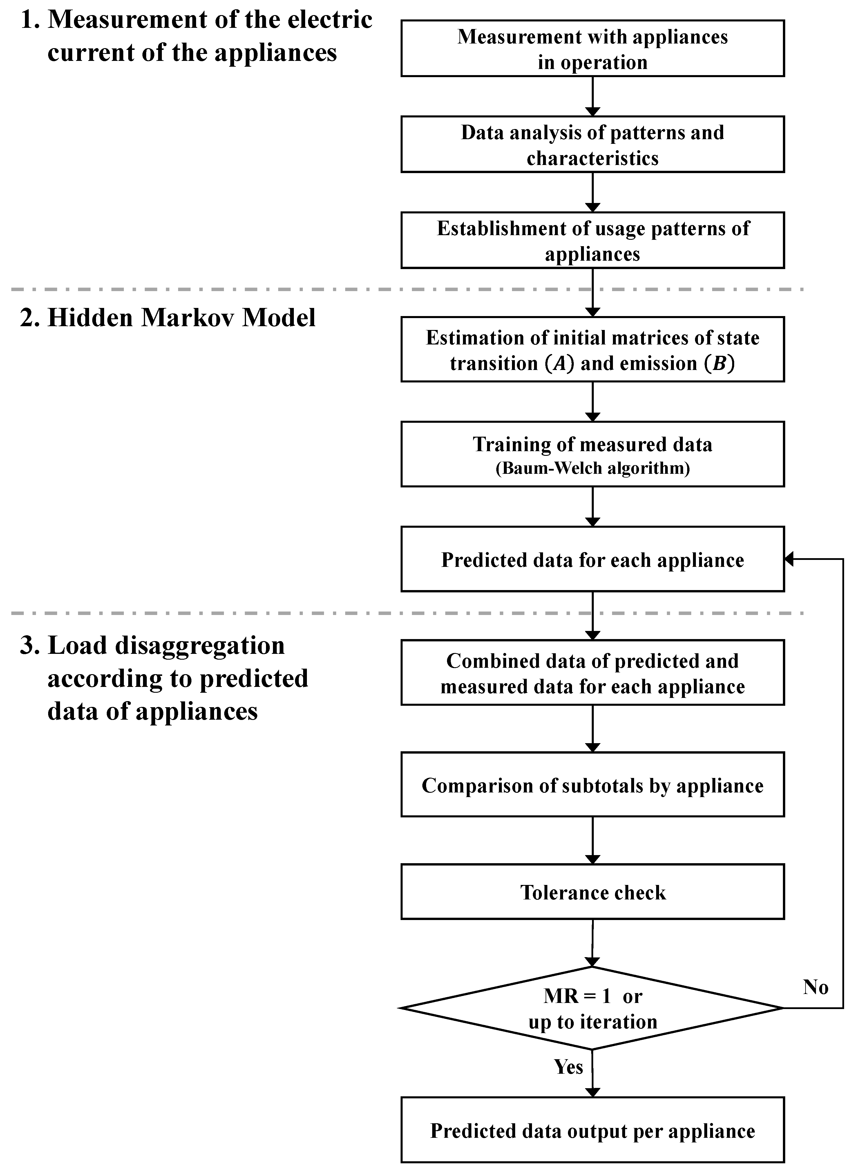
Four types of commonly used major appliances (i.e., laptops, refrigerators, TVs, and microwaves) were selected regarding their use in general residential buildings. As shown in Figure 1, the experiment was thereafter divided into three stages:
- Data were measured when the appliances were in operation. The electric current of the four types of appliances was measured using a device, and their patterns and characteristics were analyzed, classified, and determined for entry into a HMM.
- The determined pattern data for each appliance, which estimated the initial values of matrices of state transition probabilities and emission probabilities , were used as HMM input variables. The HMM was completed by being trained with the Baum–Welch algorithm, and the electric current was predicted in the completed HMM for each appliance.
- All predicted electric current data for each appliance were combined, the sum of which was compared with that of data measured for the appliance used over the course of a day. A matching rate that met the tolerance level of the measured and predicted data was calculated for all times. If the matching rate was less than one, then values within tolerance was used repeatedly for prediction; if the matching rate equaled one or repeated up to the set number of repetitions, then the process was terminated, even if the matching rate was less than one. If the error between the measured and predicted data was within the tolerance, then the load of each appliance in the measured data was considered to have disaggregated, and the predicted data for each appliance were recorded.
3.1. Measurement of Usage Data of Major Appliances
3.1.1. Measuring Equipment
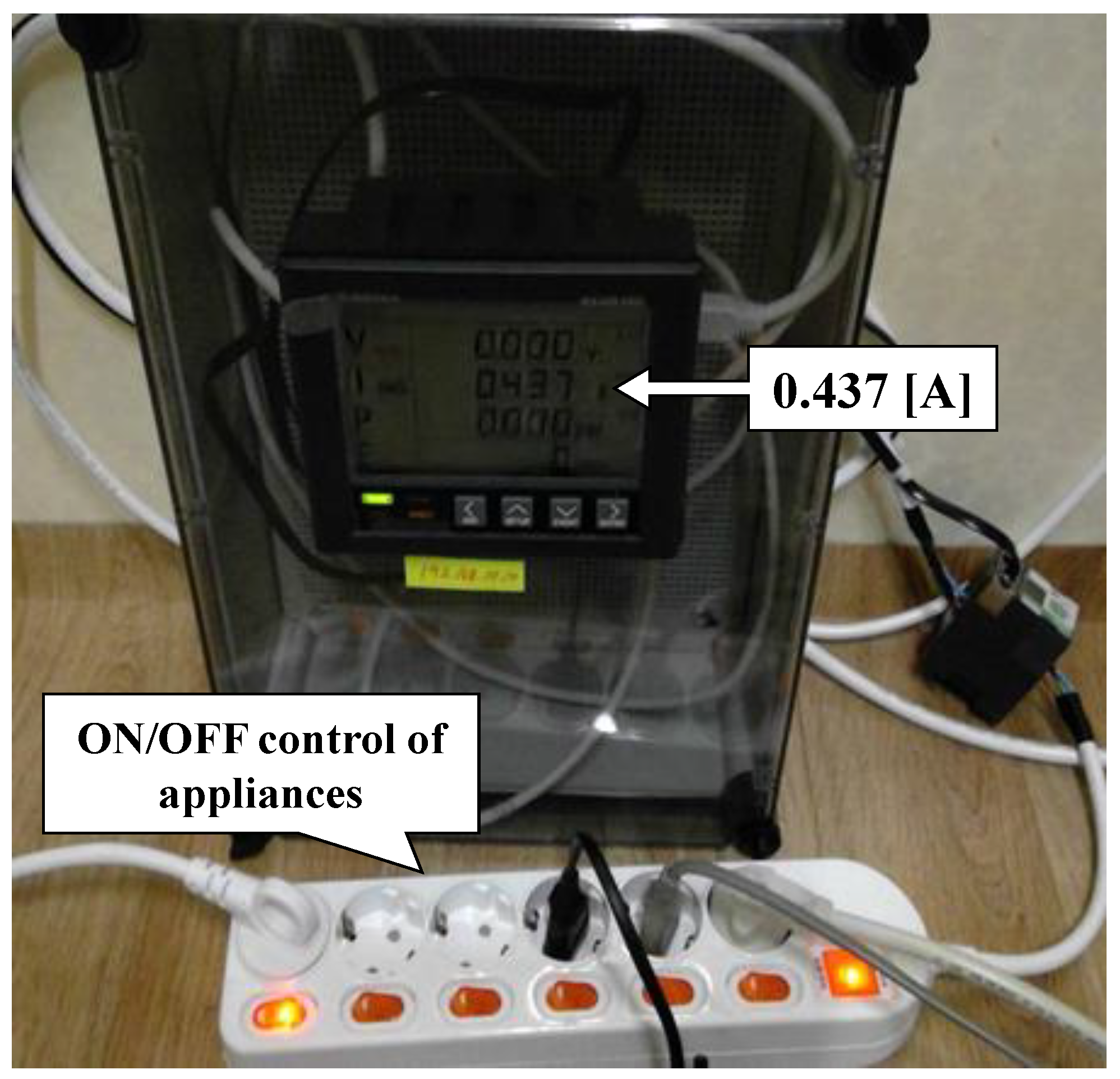
Since the load of a major appliance was predicted by recognized patterns of data, using either the power or the current was sufficient for prediction purpose. Therefore, each appliance’s electric current data were assumed to indicate the appliance’s load. In short, the method involved assuming that appliance load disaggregation was identical to that of electric current data disaggregation. For the experiment, measuring equipment was installed in the major appliances in a residential building currently inhabited. Figure 2 [26] shows the arrangement of a multi-tap and a device for measuring current data relative to whether the appliance was turned on or off. Table 3 [27] presents the specifications of the measuring equipment.
A low sampling rate is not useful for identifying change of state and thus detecting devices with low energy consumption [24]. However, devices with high energy consumption like water heaters can be accurately identified even at a sampling rate of 10 min [17]. This study was interested in devices with clear usage patterns except LT, which was assumed to be a base load. Accordingly, no expensive device was needed [10], and a low sampling rate (1 min) was applied to learn usage patterns in a practical and effective way.
3.1.2. Measurement Plan
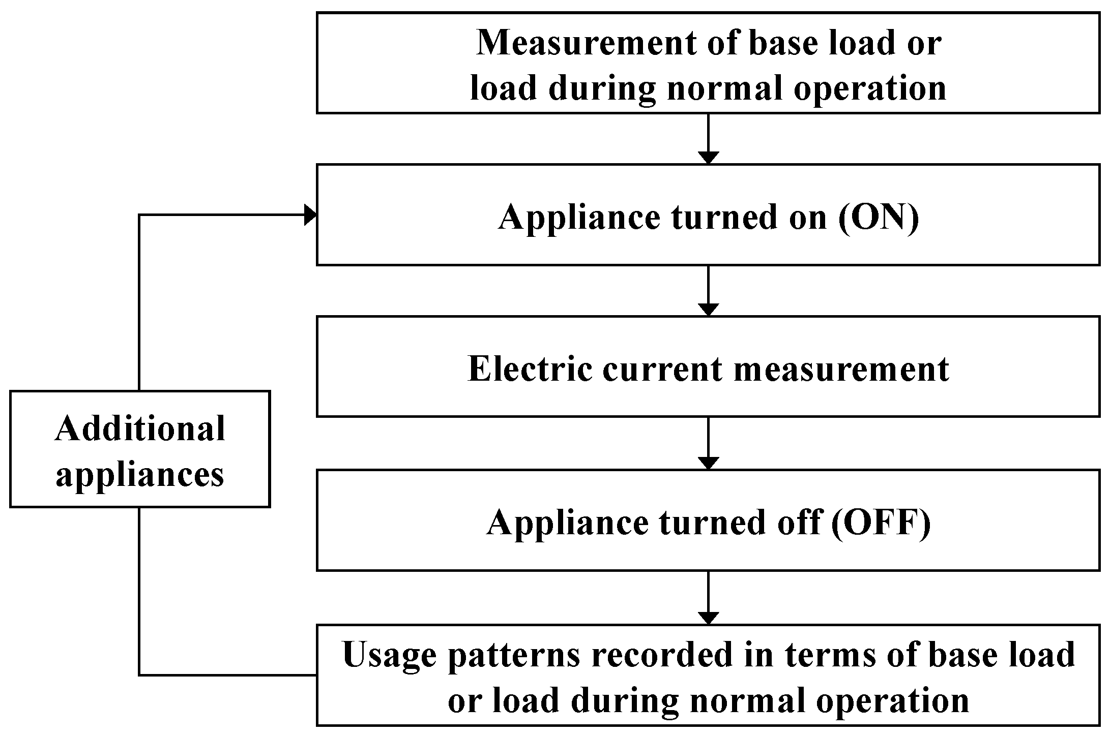
Among the variety of major appliances used in general residential buildings, four types—a laptop (LT), a refrigerator (REF), a television (TV), and a microwave (MW)—were selected for the study and their usage patterns measured. The measurement plan is shown in Figure 3. Each appliance was operated after measuring its base load or load during normal operation to subsequently measure its usage pattern during normal operation. After stopping the appliance, another appliance was operated to measure its usage pattern, and the procedure was repeated. LT was in operation at all times to collect data from the measuring equipment. LT was assumed to represent the base load or normal operating load of a general residential building, and REF, TV, and MW were additionally operated and measured. Measurement was thus performed for combinations of LT, LT + REF, LT + TV, and LT + MW.
3.2. Data Measurement
3.2.1. Measurement Data of Major Appliances for Training
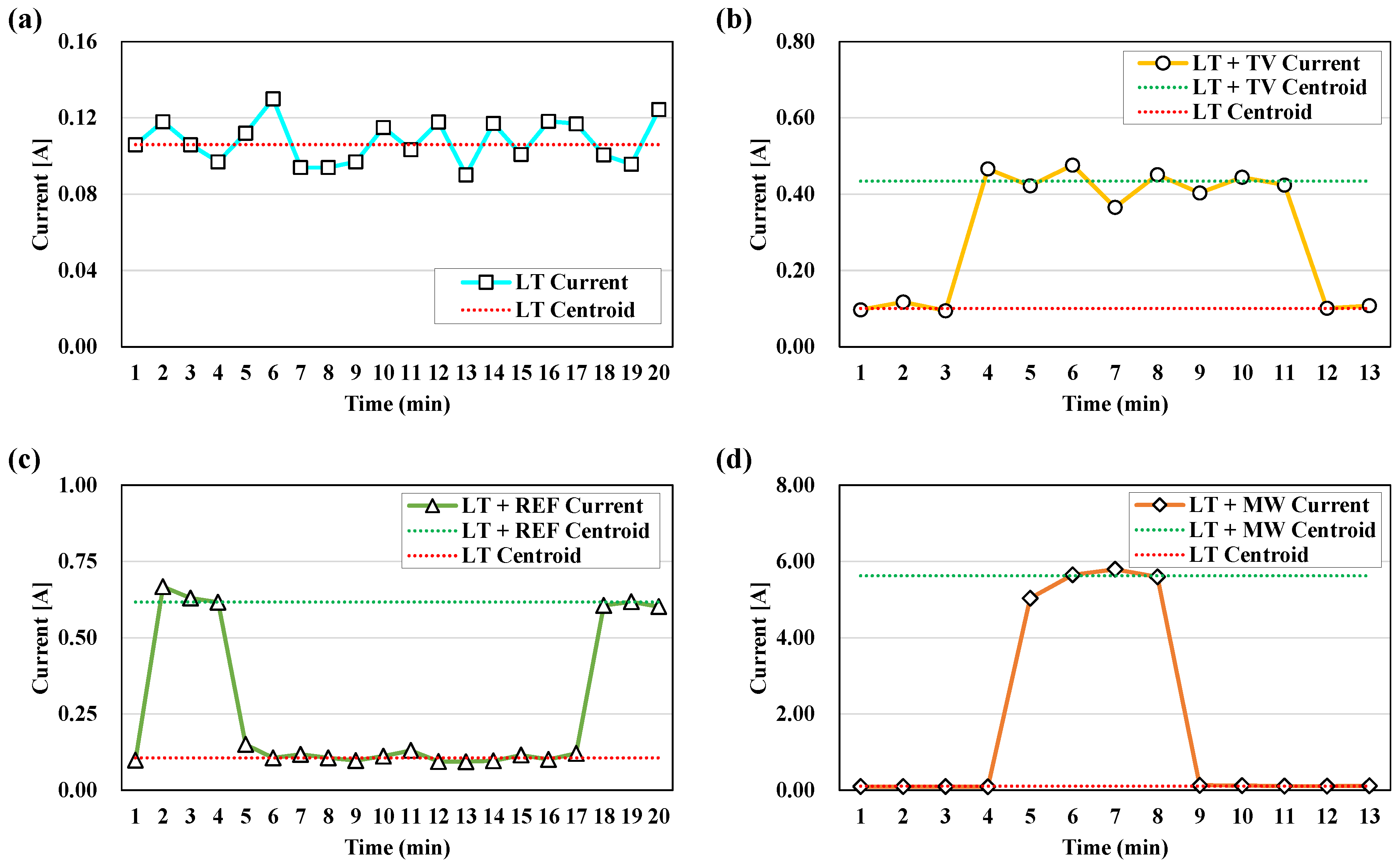
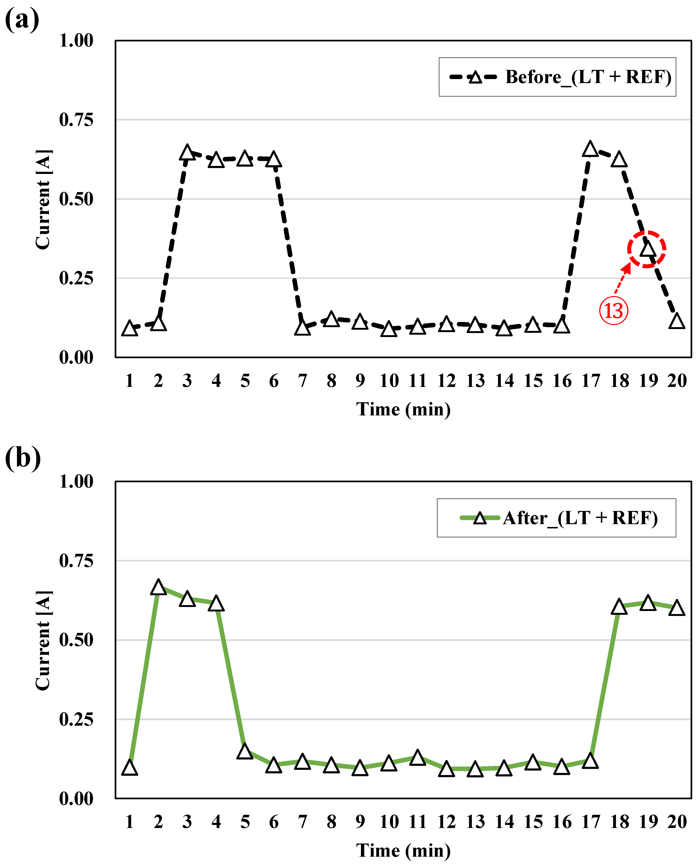
The measurement data of the major appliances, used as training data of the load disaggregation method, appear in Figure 4 for the four combinations. Figure 4a depicts the current data pattern in a state in which LT was used, measured at dawn to minimize the effects of the other appliances. In Figure 4a, the dotted line represents the centroid of LT data calculated using the k-nearest neighbor algorithm. Figure 4b depicts the current data pattern in a state in which LT + TV were used; TV was active from minutes 4 to 11, and only LT operated for the remainder of the time. In Figure 4b, the dotted line distinguishes the two appliances with their different centroids. Figure 4c depicts the current data pattern in a state in which LT + REF were used; REF was activated from minutes 2 to 4 and from minutes 18 to 20, and only LT operated for the remainder of the time. Last, Figure 4d depicts the current data pattern in a state in which LT + MW were used. MW was activated from minutes 5 to 8, and only LT operated for the remainder of the time. The current sum of MW was 50–60 times greater than that of LT, which confirms that LT’s current sum was relatively small.
3.2.2. Measurement for Load Disaggregation Verification Data
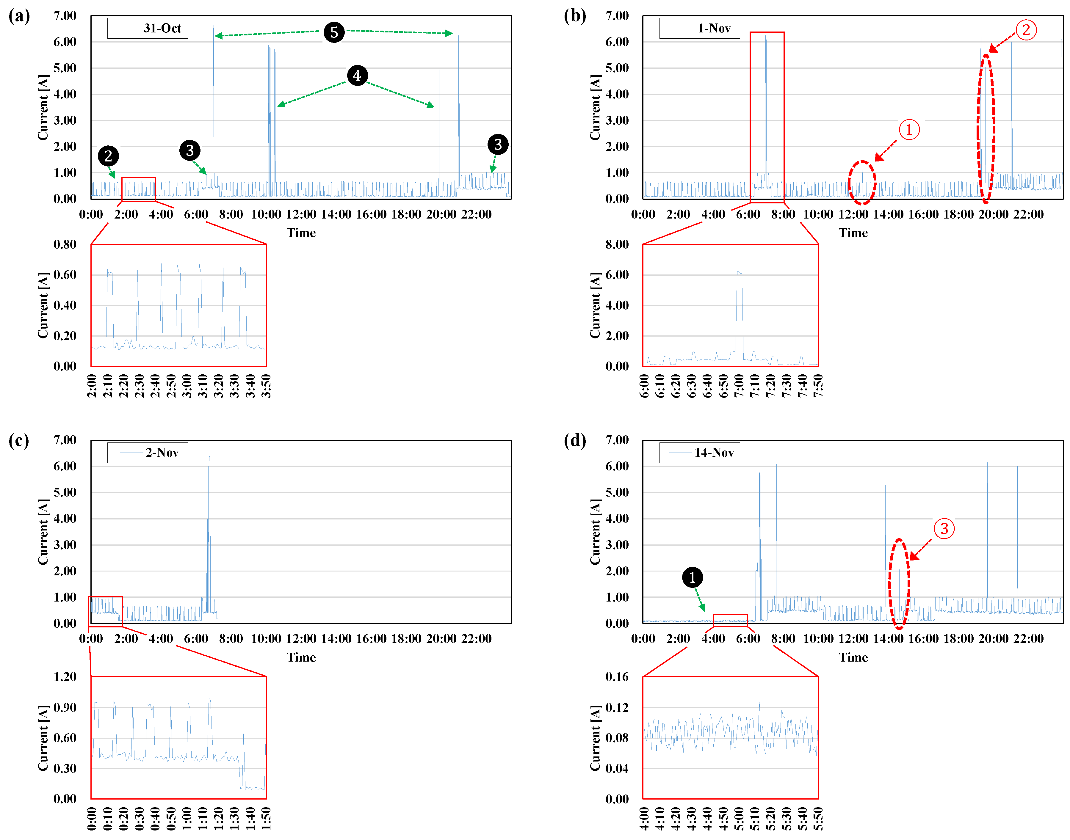
After developing the load disaggregation method, the current data of the appliances were measured for verification from the 31 October to the morning of 2 November, and on 14 November, as shown in Figure 5. Table 4 presents the usage patterns of the appliances.
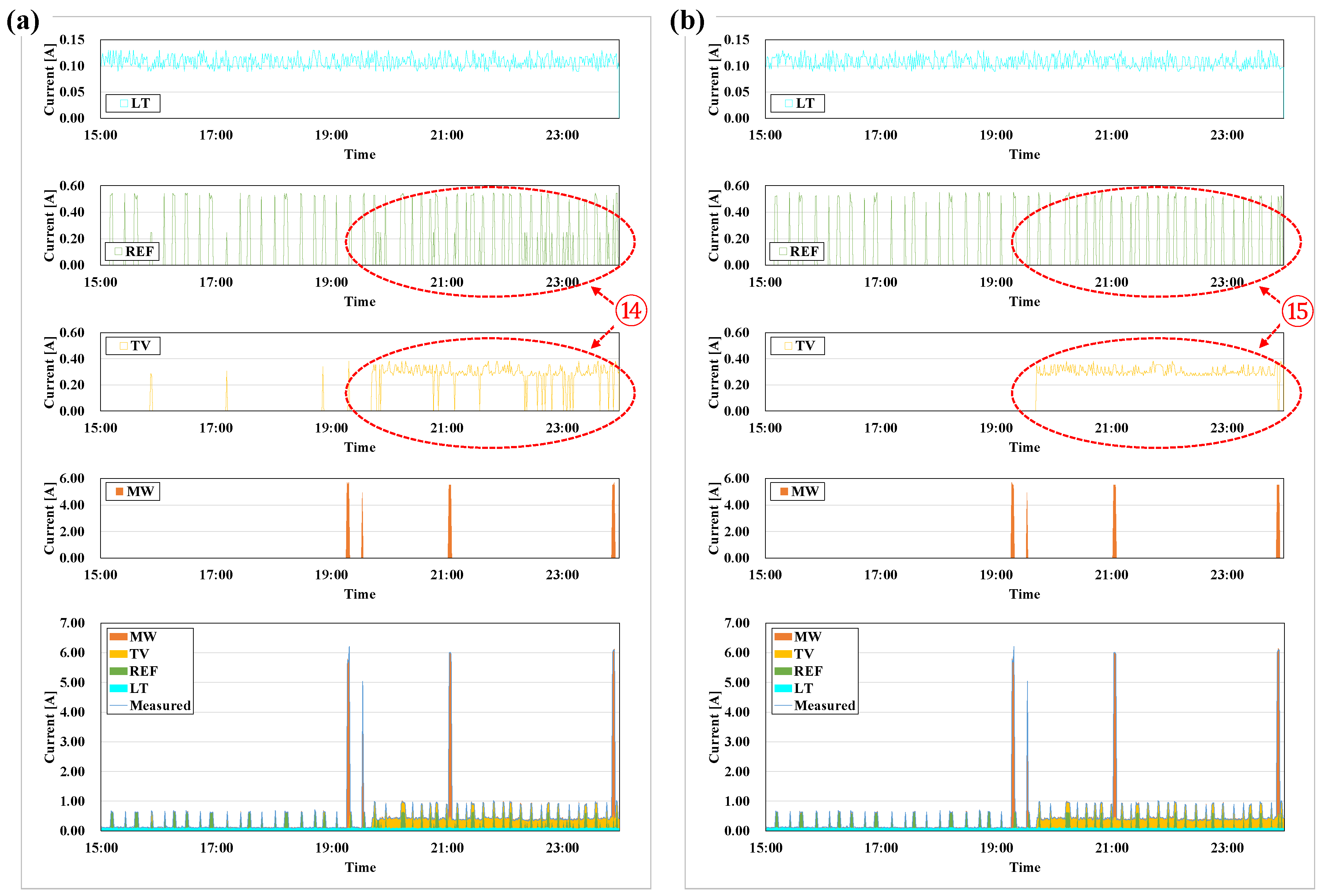
Figure 5a depicts the current data measured on 31 October, on which day only LT + REF were used from 0:00 to 6:20, TV was used from 6:20 to 7:10 and from 21:00 to 23:40, and MW was used at 7:00, from 10:00 to 10:30, at 19:55, and at 21:00.
Figure 5b depicts the current measured on 1 November. The current was measured after 31 October, and the pattern of use was similar to that measured on 31 October. Only LT + REF were used from 0:00 to 6:20, TV was used from 6:20 to 7:20, MW was used at 7:00, 19:20, 21:00, and 23:50, and TV was also on from 20:00 to 25:30 (i.e., 01:30 on 2 November). Although MW was also used for 10 s at 12:45, Figure 5b shows that use as if the outlier was measured, as shown in ①, because the measurement interval was 1 min. Similarly, ② was measured for MW for 50 s, which was approximately 1 A less than a typical MW usage pattern.
Figure 5c shows the current measured on 2 November continuously after 1 November; its usage pattern was similar to that of the morning of 1 November. Only LT + REF were used from 0:00 to 6:20, TV was used from 6:20 to 7:10, and MW was used at 6:50. After the morning hours, measurement was not made due to errors in the measuring equipment.
Last, Figure 5d shows the current measured on 14 November, on which day only LT was used from 0:00 to 6:20. In that case, unlike in the previous measurement, REF was not measured due to a connection error with the measuring equipment. Once the error was fixed, REF was connected to the measuring equipment at 7:05. TV was watched continuously from 7:05 to 10:10, intermittently at 15:00, and continuously after 17:00. MW was used at 6:30, 7:30, 13:50, 19:50, and 21:40; MW was also used for 30 s at 14:45, but the outliers appeared as shown in ③ because the measurement interval was 1 min.
3.3. Hidden Markov Model (HMM)
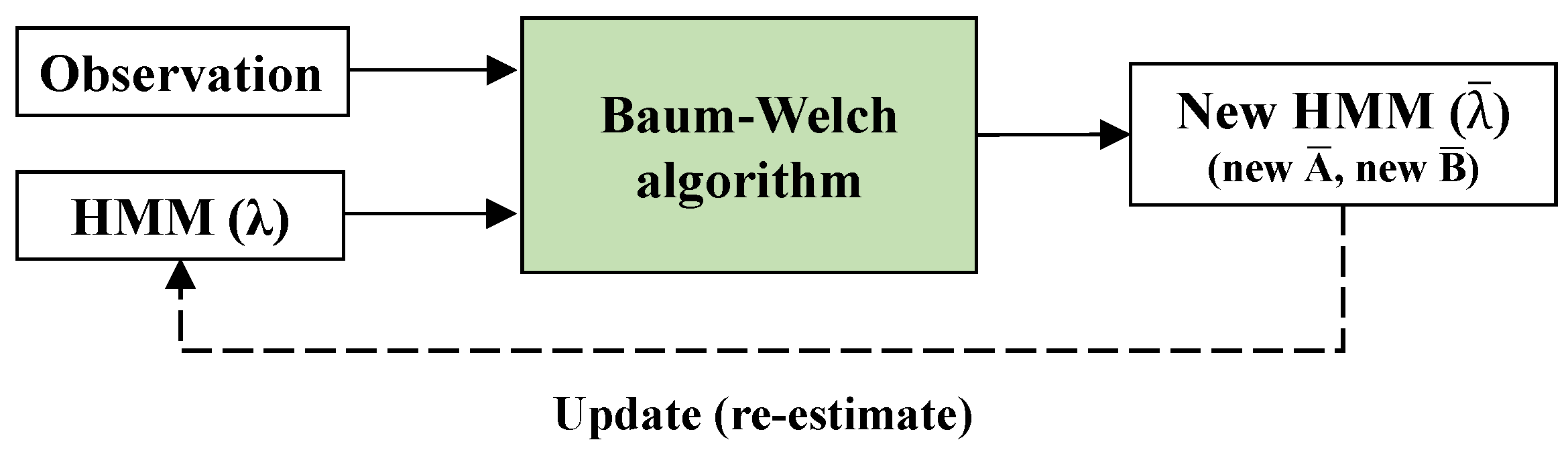
Using the HMM required observation (emission) and state transition data; observation data refer to electric current, and state transition data refer to the on or off state of each appliance. Using those two types of data, we calculated the input variables and for the model. Once the initial values were estimated, they underwent HMM updating (or re-estimation). HMM updating uses the Baum–Welch algorithm, which requires inputting the observation vectors and the initial HMM model (i.e., initial input variables A and B), as shown in Figure 6. The observation vectors indicate that the observed data can be multiple sets. New vectors and were derived using the Baum–Welch algorithm, and ultimately, the HMM model was determined [28].
3.4. Load Disaggregation by Predicting the Electric Current of Appliances
The predicted data were compared with the measured data, and an error was calculated by using Equation (1). Next, using Equation (2), whether the error was within the tolerance was examined. The matching rate was calculated by comparing the time (number of time segments) that met the tolerance and the time (number of time segments) of the measurement data using Equation (3). The data of each appliance were re-entered into the prediction using the HMM until the matching rate became 1 or the number of iteration was repeated. If the electric current was not predicted to be within the allowable error despite being repeated up to the number of iterations, or if the measured data were ‘0’, then the predicted data were determined to be ‘0’ as the output. By contrast, if the error between the predicted and measured data was within an allowable error for a given time, then the sum of the electric current of the respective appliances was considered to be approximate to that of the measured data. Therefore, the predicted current data of each appliance resulted from disaggregating the measured data. In other words, if the matching rate was 1, then the predicted data of all of the measured times was the result of disaggregating the measurement data; if the matching rate was 0.8, then the predicted data indicated the result of disaggregating the measurement data by only 80% of the total measured time. For example, if the measurement time was 10 minutes and the total number of errors (in the measurement and predicted data) that were less than the tolerance (i.e., the number of times at of 1) was 8, the number of errors within the tolerance (8) was divided by 10, assuming that the measurement interval was 1 min at Total 10, and the matching rate was calculated as 0.8 (8/10).
where is the error, is the measurement data, is the predicted data, is the LT’s predicted data, is the REF’s predicted data, is the TV’s predicted data, is the MW’s predicted data, is the probability whether the error is within the tolerance (1 if within the tolerance; 0 if otherwise), is the tolerance, is the matching rate, is the number of measurement data, is the measured times, and is the th measured time.
3.5. Algorithm Platform Development Environment
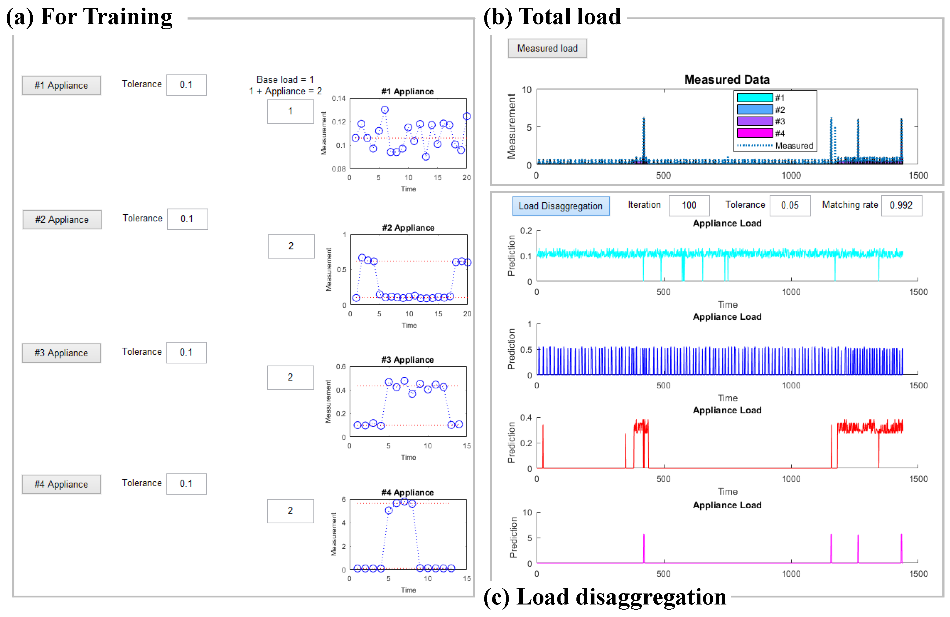
As shown in Figure 7 [26], a load disaggregation algorithm platform was developed using a MATLAB-based graphical user interface (GUI) (R2017a, MathWorks, Seoul, Korea). This platform consists of measurement data input for training (Figure 7a), total load data input for disaggregation (Figure 7b), and output for the disaggregated loads of each appliance (Figure 7c). In addition, HMM-related functions such as hmmestimate, hmmtrain, and hmmgenerate were used to develop the algorithm.
In Figure 7a, the training input measurement data from the first appliance (#1 Appliance) was LT, assumed to be the base load. Next, the second appliance (#2 Appliance) input measurement data of LT + REF. The third appliance (#3 Appliance) input measurement data of LT + TV. The fourth appliance (#4 Appliance) input that of LR + MW. The graph of measurement data for training had the ON/OFF distinction and marked the centroid with a red dotted line. In Figure 7b, the entire measurement data of a single day for load disaggregation was input. In Figure 7c, an iteration number of 100 and allowable error of 0.05 were input as defaults for load disaggregation, but these can be modified by users. When the load disaggregation button is pushed, the procedure of Section 3.4 is implemented to predict LT, REF, TV, and MW, thereby calculating MR.
4. Case Study and Results
4.1. Case 1: 31 October (0:00–23:59)
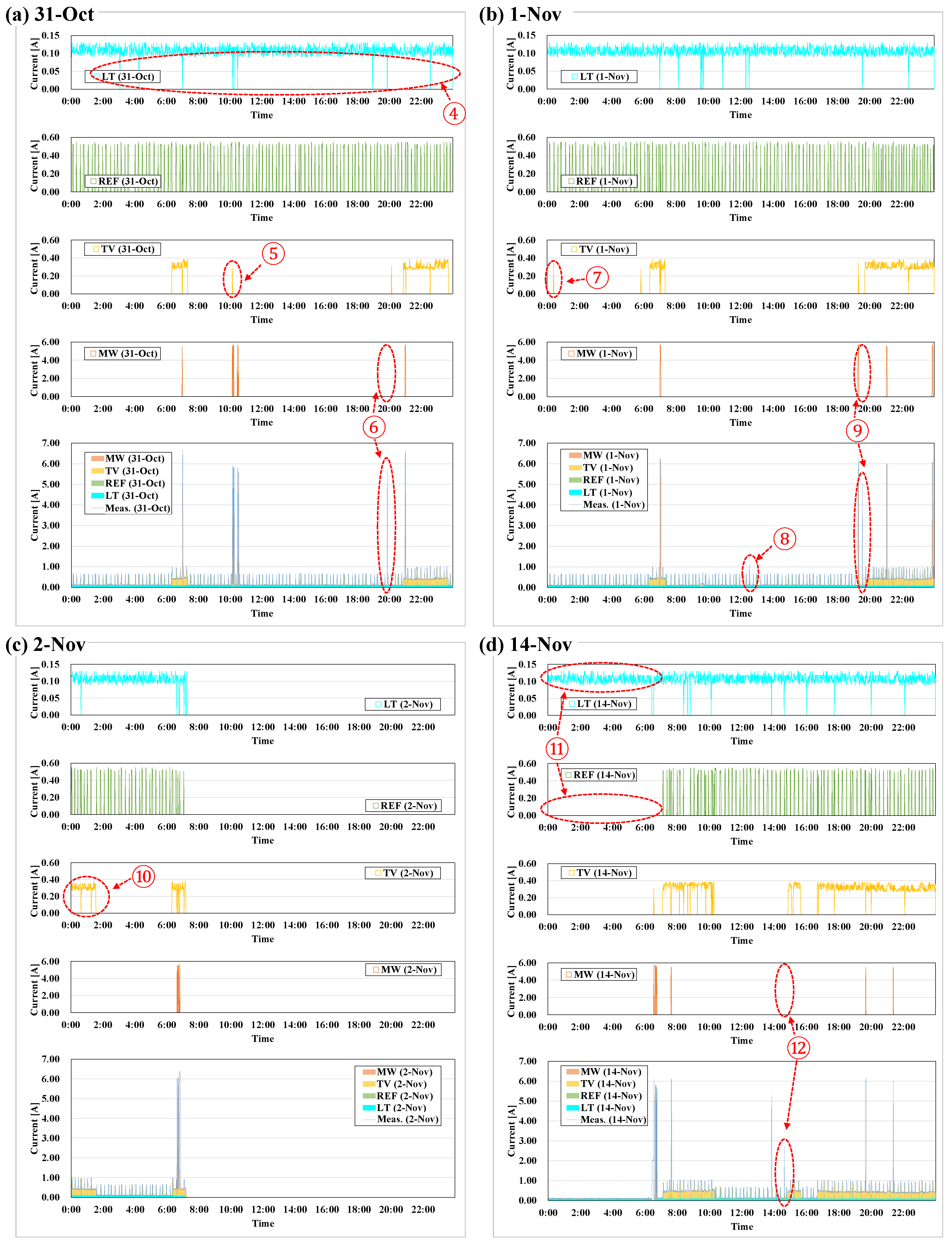
Figure 8a shows the results of load disaggregation with the measurement data from 31 October. The number of repetitions was set to 100, and the tolerance was set to 0.05. As a result, the MR of the measured and predicted data was calculated to be 0.994 (1431/1440), because the MR was calculated to be nine times of ‘0’, as shown in ④ of Figure 8a when LT was disaggregated. Accordingly, the error of measured and predicted data not within the tolerance was derived nine times, and LT, REF, TV, and MW all output 0. Conversely, LT and REF were used continuously throughout the day, and TV was operated in the morning and evening hours. As shown in ⑤ of Figure 8a, however, the predicted value of TV at about 10:00 was the median of REF. (Intermediate values are described in Section 4.1). MW was used at breakfast and at around 10:00, 20:00, and 21:00; the use of MW was not predicted, as shown in ⑥, because it was not predicted using the HMM, the tolerance with the measured data was not met, and the result was ‘0’ as output. Since the predicted data were derived stochastically in a separate HMM for each appliance, values might not have been predicted within the tolerance at all times. If as many iterations were performed as possible, then a value within the tolerance was possible with longer running time.
4.2. Case 2: 1 November (0:00–23:59)
Figure 8b shows the results of load disaggregation with the measurement data from 1 November. The number of repetitions was set to 100, and the tolerance was set to 0.05. As a result, the MR of the measured and predicted data was calculated to be 0.992. Similar to Case 1, the load disaggregation output ‘0’ because the error of measured and predicted data was derived to be not within the tolerance. On the other hand, LT + REF were used continuously throughout the day, whereas TV was operated in the morning and evening hours. As shown in ⑦ of Figure 8b, however, TV was operated at dawn because the median value of REF was measured as a result, the same as in ⑤ in Figure 8a. ⑧ of Figure 8b shows the same case as ① of Figure 5b, in which ‘0’ was the output because the error of the measured and the predicted data was not within the tolerance. MW was operated during the breakfast, dinner, and midnight hours. ⑨ of Figure 8b shows that the error of the predicted data of MW operated before the evening hours was not within the tolerance with the measurement data, resulting in ‘0’ output. This is the same as ② shown in Figure 5b (See Section 3.2.2).
4.3. Case 3: 2 November (0:00–7:13)
Figure 8c shows the results of load disaggregation with the measurement data of 2 November. The number of repetitions was set to 100, and the tolerance was set to 0.05. As a result, the MR of the measured and predicted data was calculated as 0.982. Similar to cases 1 and 2, the load disaggregation output ‘0’ because the error of measured and predicted data was derived to be not within the tolerance. On the other hand, LT + REF were operated continuously throughout the measurement, whereas TV was watched until the middle of the night following the previous day (1 November) as shown in ⑩ of Figure 8c and watched in the morning (6:20–7:13). The measured MW shows frequent usage at breakfast hours. The error with the predicted data met the tolerance in some cases, and sometimes not, resulting in ‘0’ output.
4.4. Case 4: 14 November (0:00–23:59)
Figure 8d shows the results of load disaggregation with the measurement data of 14 November. The number of repetitions was set to 100, and the tolerance was set to 0.05. As a result, the MR of the measured and predicted data was calculated as 0.988. Similar to the previous cases, the load disaggregation output ‘0’ because the error of measured and predicted data was derived to be not within the tolerance. As shown in ⑪ of Figure 8d, LT was operated continuously throughout the day, whereas REF was operated from the morning (7:05) hours (see Section 3.2.2). TV was operated from morning to afternoon, and from evening to late night. The MW was frequently operated at breakfast, and also in the afternoon and evening. However, the MW of 13:50 did not output because the error of measured and predicted data was not within the tolerance. Also, ⑫ of Figure 8d shows that the MW was used for only 30 s, the same as in ③ of Figure 5d. The error with the measured and predicted data was not within the tolerance, resulting in ‘0’ output (Section 3.2.2).
4.5. Performance Metrics
The performance of the load identification of this algorithm was assessed in terms of such metrics as accuracy, precision, recall and F-measure using the well-known Equations (4)–(7) [22,24,29].
where is the true positive, is the false positive, is the true negative, is the false negative.
One of the remarkable characteristics of the proposed algorithm is that it does not identify each appliance but a combination of appliances based on measured energy consumption, and it then disaggregates this data into each appliance. Accordingly, if a combination of appliances is identified, only a true positive is confirmed. On the other hand, if no combination of appliances is identified, only a false negative is confirmed. Consequently, the precision is always 1 and the accuracy and recall have the same result as MR. Table 5 summarizes the identification performance, which was tested for four days.
5. Discussion
5.1. Conditions of Training Data
As mentioned above, this study measured the usage patterns of appliances every minute and used the measurements as the training data for HMM. However, not all appliances have such discrete operation as to be detected every minute. For example, as shown in of ⑬ in Figure 9a, REF operated for only 24 s and then stopped. At this time, the current was measured to be 0.34 A. This value is less than the typical value measured during a 1 min operation of REF; that is, it indicates a median. In that case, the median value refers to data measured for a time less than the measurement interval of 1 min, not the middle value. As a result of load disaggregation after training with data from Figure 9a, the median value of REF and the frequent turning on and off of TV were obtained, as shown in Figure 10a. Data of REF shown in ⑬ of Figure 9a were similar to data of TV. Consequently, results shown in ⑭ of Figure 10a were used because REF or TV might have been predicted to operate when being predicted in an HMM model. It is therefore necessary to measure the training data of REF shown in Figure 9b again. Compared with the training data in Figure 9b, those in Figure 9a showed a slightly different pattern without a median value. After disaggregating the loads of LT + REF as the modified training data shown in Figure 9b, however, REF + TV were predicted for results shown in ⑮ of Figure 10b. In contrast with ⑭ of Figure 10a, the REF did not show a median value such as in ⑮ of Figure 10b, and TV was not frequently turned on and off. In the training pattern shown in Figure 9a before modification, the load disaggregation did not yield an accurate prediction due to the interference of REF + TV; conversely, in the modified training pattern shown in Figure 9b, the load disaggregation of REF + TV was clearly performed. Therefore, it is also necessary to measure the training data in the HMM with the characteristics of each appliance clearly classified. Regarding other results, ⑤, ⑦, ⑧, ⑨, and ⑫ of Figure 8 show the median values of the current measured. Those values cannot be predicted when training HMM with pattern data in which no median values exist, as shown in Figure 4, because all corresponding parts emerged as ‘0’ output, as shown in Figure 8. However, when training with median values included, results similar to those in ⑭ of Figure 10a emerged. Additional studies are thus needed to clarify that dynamic, because the training data and measurement intervals of data operated within a tradeoff relationship.
5.2. Iteration
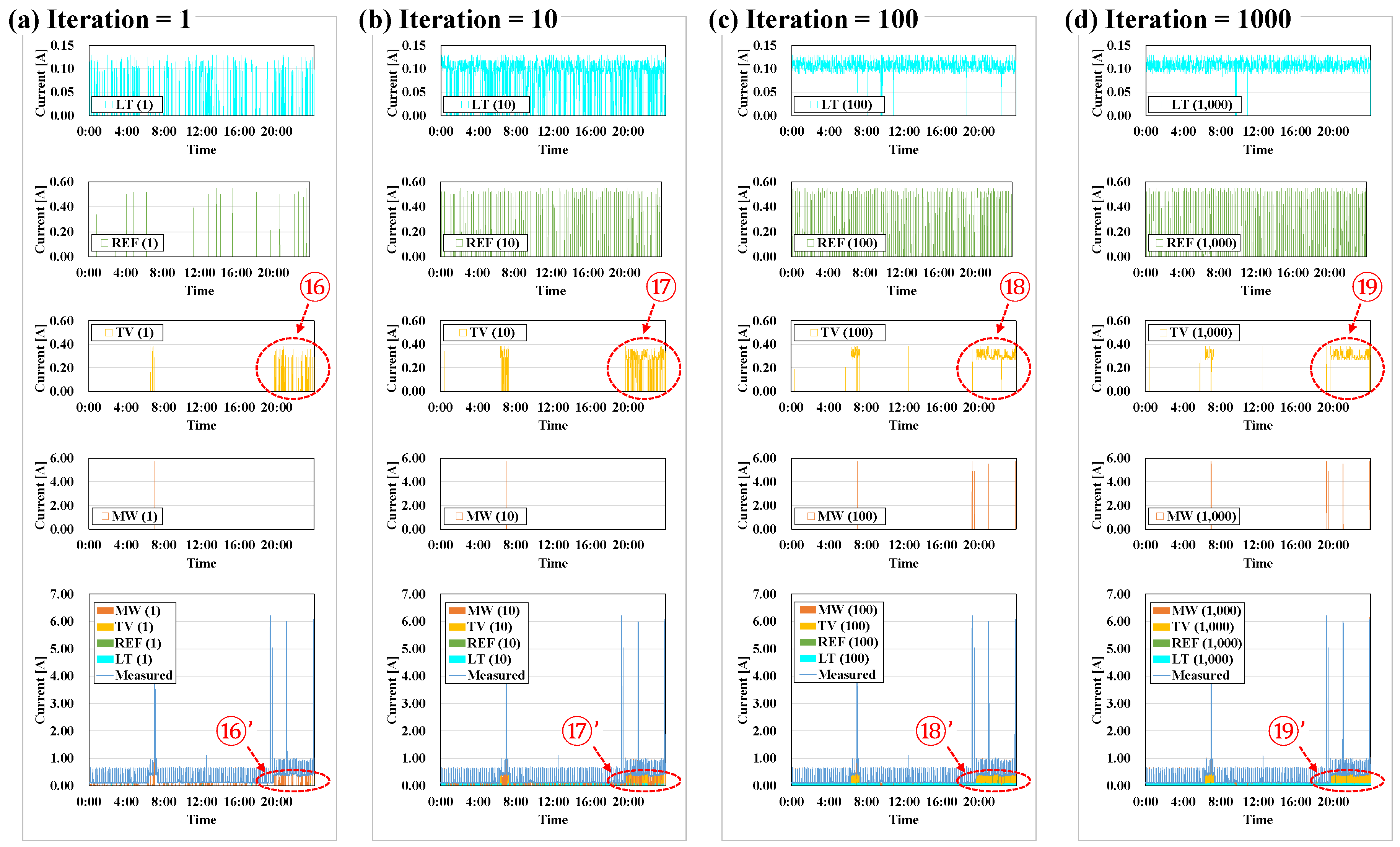
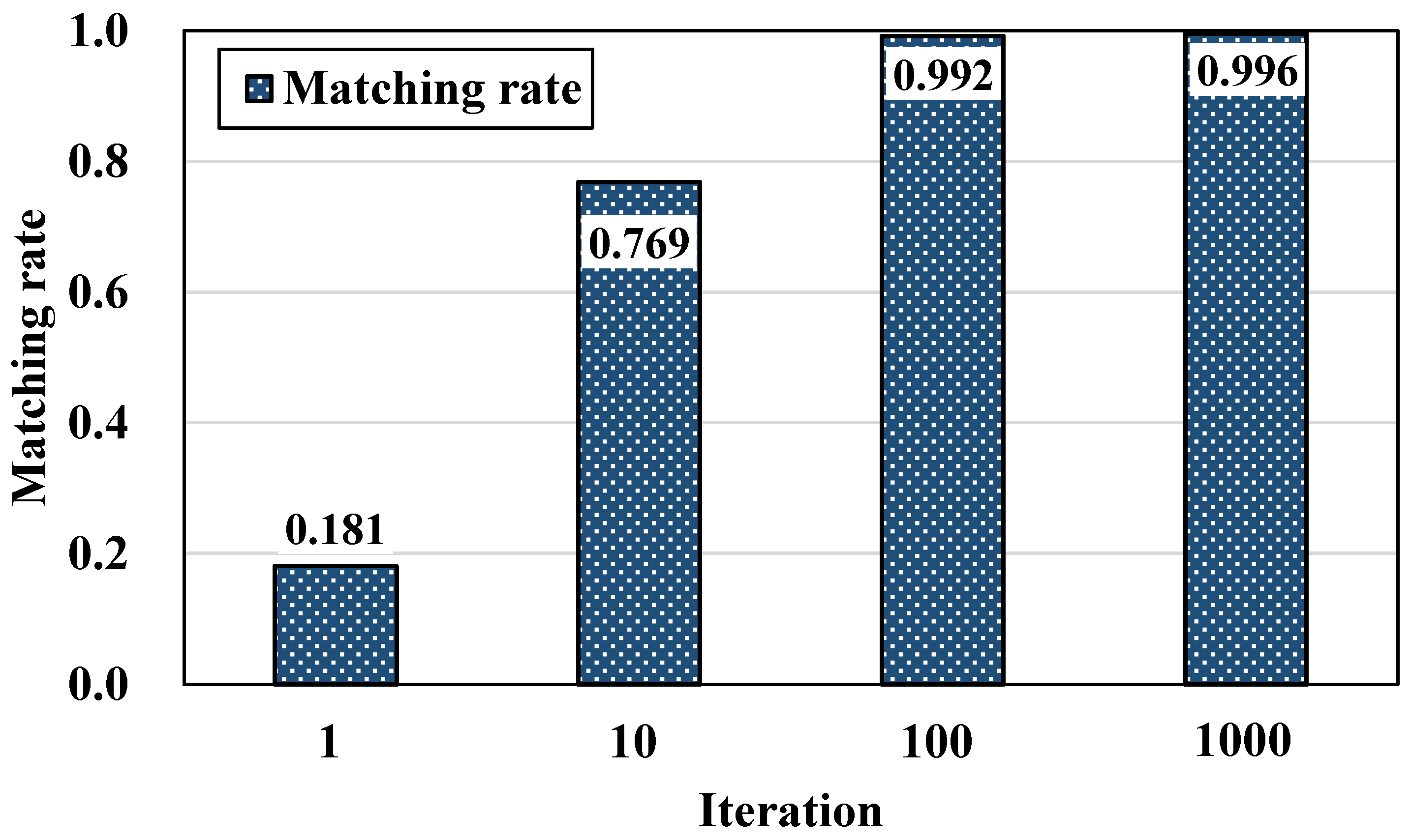
Because the HMM is a probability model, the predicted data might not have been approximated to the measurement data. Therefore, the iteration method was chosen to supplement the HMM’s inherent limit. Here, iteration refers to the number of times the predicted data were repeatedly calculated with the HMM when the matching rate was less than ‘1’. Figure 11 shows the results of the load disaggregation of the major appliances by repetition frequency. The greater the number of iterations, the more approximate to the measured data the predicted data were. That TV was predicted as ⑯→⑰→⑱→⑲, as shown in Figure 11, suggests that it approached measurement data shown to be ⑯’→⑰’→⑱’→⑲’. However, it is necessary to determine the optimal number of repetitions because the running time lengthens as the number of repetitions increases. Figure 12 shows the results of examining the matching rates of the load disaggregation outcomes of the major appliances by repetition frequency. When the number of repetitions was small, the matching rate was not high, however, when the number of repetitions was 100 or more, the matching rate showed a value of at least 0.99. Therefore, the number of iterations was set at 100 as a default, even though the number of repetitions is designed to be entered differently depending on the situation.
5.3. Tolerance
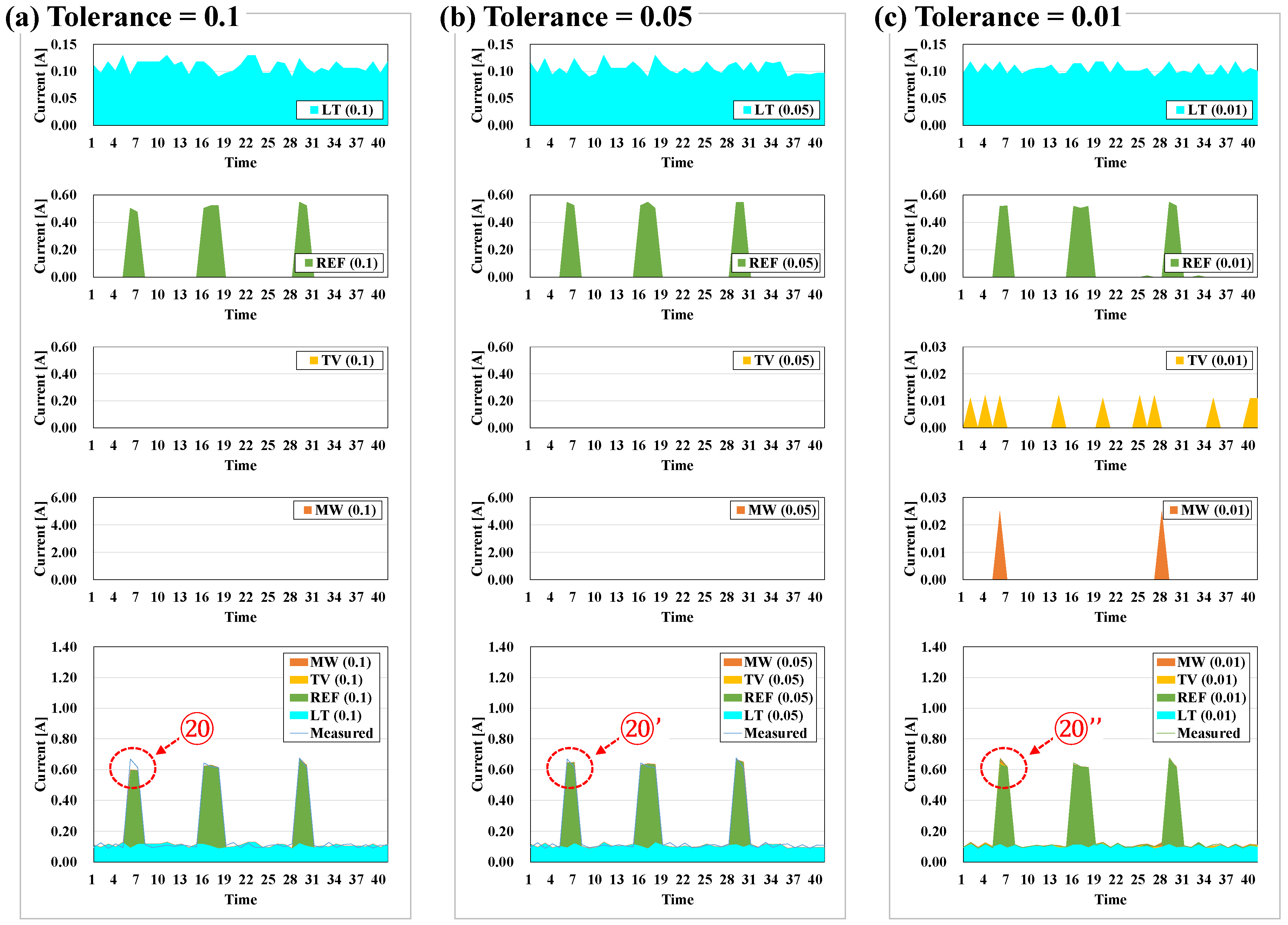
In the method developed, tolerance was used as a criterion for examining the error of measurement data and predicted data via a matching rate calculation. Figure 13 shows the load disaggregation of LT + REF in terms of tolerance. The smaller the tolerance value, the more likely it is to produce the predicted output data in close proximity to the measurement data, as shown in ⑳, ⑳’, and ⑳’’ of Figure 13a–c. However, major appliances other than LT + REF were produced in ⑳’’ of Figure 13c. With less tolerance, the prediction data were closer to the measurement data, however, if the tolerance is inadequate, then different results can occur. Therefore, tolerance was set at 0.05 A, which could separate the characteristics of the load and preclude such results. Again, however, tolerance is designed to be entered differently depending on the situation.
5.4. Applicability Review
As an examination of the applicability of the load disaggregation method developed in the study revealed, additional research is needed to improve the method in four aspects.
- The current algorithm should measure the training data so that the characteristics of the load are clearly classified. It is necessary to compensate for the data with intermediate values so that the characteristics of the training data can be discriminated by varying the measurement interval.
- The greater the number of iterations, the fewer the errors and the higher the matching rates, but the execution time of the algorithm becomes longer. Therefore, an additional algorithm for determining the optimal number of iterations is necessary.
- The tolerance should be set to fall within the load disaggregation but not be too limited. When disaggregating the load for major appliances other than the ones examined in the study, however, it is necessary to check the scale of the measurement data. Among the appliances examined, all but MW had tolerance of less than 1 A, and tolerance was therefore set at 0.05 A. However, for appliances whose data were measured to be greater than 1 A, tolerance should be greater than the presently set tolerance because a minimal tolerance that remains within the tolerance is pivotal to increasing the performance of load disaggregation.
- If untrained patterns or outliers are detected, then response measures require greater flexibility.
5.5. Contribution and Limitation
This study includes the following contributions, potential improvements, and limitations.
Sampling rate. A high frequency rate (0.02 s or less) enables current–voltage waveforms as well as energy to be analyzed. High frequency data can be obtained with a special monitoring device, and a lot of computational and communication power are needed to process the data [24]. A low frequency rate (1 s or more) is easily achievable without using an expensive device. Since changes of state may not be visible at such a low frequency rate, devices with low energy consumption are difficult to detect [24]. However, a water heater and other devices with high energy consumption can be correctly identified at a sampling rate of 10 min [17]. As compared to high sampling rates, low sampling rates do not need an expensive device and are a more practical and promising methodology [10]. This study applied a low sampling rate (1 min) for the training of usage patterns in order to identify appliances.
Privacy. Perhaps, the biggest challenge of NILM is not technology but privacy [10,17]. Scalability is to be allowed while minimizing the expenses of sensor installation, data collection/analysis, and privacy protection [30]. This study considered privacy issues from two perspectives. The first is the above-mentioned sampling rate. A high sampling rate can provide detailed information [10]. On the other hand, a low sampling rate has a lower identification accuracy but is less susceptible to privacy issues. The second one is identifying appliances based on a combination of usage patterns, as shown in Figure 5 and Table 4. If a combination of appliances is identified, multiple appliances are identified together, which seems to be less likely to create privacy issues than the identification of individual appliances. However, only normally operating devices out of the combination, not malfunctioning ones, could be identified.
Identification and Training. In case a user wants to add a new appliance or modify an existing one, this algorithm measures usage patterns, as shown in Figure 4, and inputs the data into the setup shown in Figure 7a, thereby being able to be retrained at any time. In other words, the proposed algorithm is flexible with the modification of training data. However, unlike training and retraining, malfunctions or other patterns of energy consumption (current in this study) cannot be identified. For example, in ①, ②, and ③ of Figure 6, the real measurements did not have the previously trained patterns but different patterns of energy consumption (current). These sections cannot be identified as ⑧, ⑨, and ⑪ of Figure 8. Two solutions to this problem are worthy of consideration. First, if appliances have to be identified using unknown patterns or values, an intelligent guess is used or the most similar appliances are identified [15] and the information is provided to users in the form of an alarm. Second, online training is available. If usage patterns for signatures are saved in real time in a database and updating is possible through online self-training, both malfunctions and other patterns of energy consumption (current) can be identified. Besides, when the efficiency of an appliance is degraded or the initially trained-for pattern is changed, such modifications can be retrained and identified. Moreover, a comparison with the initial state stored in the database could alert the user to a need for replacing the device, which could bring economic benefits. On the other hand, the initial cost of building a database is inevitable.
Load management. In case the ON/OFF control is implemented, which considers changes in users’ behavior patterns or electrical charges, the proposed method can be applied. The identification of appliances is possible for load shifting and load shedding, which are techniques of smart grids and demand response. For example, the TV in Figure 8a was not used from 0:00 to 1:30, but had the usage pattern of ⑩ in Figure 8c. This case shows a change in the user’s behavior or load shifting. The proposed algorithm could identify this TV. In addition, if an appliance that has always been switched on becomes unused, it corresponds to load shedding. Like ⑪ of Figure 8d, LT and REF had always been switched on and only REF stopped operating. The proposed algorithm could identify this case. Accordingly, even when electrical charges change in real time in a smart grid or demand response system or users modify their patterns, it is possible to identify which appliance is being used and when. Such conditions can be satisfactorily dealt with.
Number of appliances. This study assumed that four appliances (including the base load) were operated simultaneously. However, a larger number of appliances are used in a real residential building. As the number of appliances operating simultaneously increases, the usage patterns of each appliance to be identified become more diverse and the duplicated use of appliances may increase distorted signals [31]. Future work needs to examine the identification accuracy by applying the proposed algorithm to more appliances.
6. Conclusions
In this study, a novel method of disaggregating loads of major appliances was developed and its potential examined. The usage patterns of each appliance were recognized and trained in an HMM, and their predicted and measurement data were compared. If the measured data were within the tolerance of each appliance, then the predicted data of each appliance were determined to result from disaggregation by using the measurement data. The method was reviewed for four days, and the primary results are summarized in what follows.
- The electric current of four types of major appliances was measured in a residential building currently inhabited. Data were measured when an appliance was in operation. For LT, the base load or normal operating load of a general residential building was assumed, and measurement was performed for combinations of LT, LT + REF, LT + TV, and LT + MW. Measured data were used as training data of load disaggregation.
- Measured data were updated (i.e., re-estimated) by using the Baum–Welch algorithm, and the current data of the appliances were predicted using the HMM. Errors in predicted and measured data were checked for whether they fell within the tolerance. That process was repeated to obtain predicted data whose values were approximate to those of the measured data.
- The results were examined and reviewed for 4 days: 31 October and 1, 2, and 14 November. Respective matching rates of 0.994, 0.992, 0.982, and 0.988 were achieved.
- The applicability of the load disaggregation method developed in the study was examined, and results revealed that additional research is needed to improve the measurement method for training data, to add an algorithm to determine optimal iteration, and to determine a tolerance. Flexible measures should also be secured in the case that unexplored patterns or outliers are detected.
Many older buildings require load disaggregation to accommodate policy seeking substantial energy savings in residential buildings. The proposed method can provide insights into how and where within such buildings energy is consumed. As a result, effective and systematic energy saving measures can be derived even in buildings in which monitoring sensors and measurement equipment are not installed. When installing building energy management systems, the initial building cost can be reduced because measurement equipment is unnecessary. The energy consumption of buildings can be easily examined to allow the provision of energy saving guidelines to facilitate appliance replacement and maintenance. Last, it is expected that the application of South Korea’s National Integrated Building Energy Management System (NIBEMS) will extend the scope of this method and use it to analyze the energy pattern of residential buildings of NIBEMS and to disaggregate energy load by usage.
Acknowledgments
This research was supported by a grant (18AUDP-B099686-04) from the Architecture & Urban Development Research Program funded by the Ministry or Land, Infrastructure and Transport of the Korean government.
Author Contributions
Younghoon Kwak developed the methodology with algorithms, performed the simulation, and wrote the full manuscript; Jihyun Hwang performed the experiments, discussed the results, and implications at all stages; Taewon Lee advised all tasks, double-checked the results and the whole manuscript. All authors proof read the paper.
Conflicts of Interest
The authors declare no conflict of interest.
Acronyms and Abbreviations
| DTW | Dynamic time warping |
| FHMM | Factorial Hidden Markov Model |
| FN | False negative |
| FP | False positive |
| GP | Generic programming |
| GUI | Graphic user interface |
| HMM | Hidden Markov Model |
| K-NN | K-nearest neighbors |
| k-NNR | k-nearest neighbors rule |
| LT | Laptop |
| MR | Matching rate |
| MW | Microwave |
| NILM | Non-intrusive load monitoring |
| NN | Neural network |
| REDD | Reference energy disaggregation dataset |
| REF | Refrigerator |
| SVM | Support vector machine |
| TC | Temporal correlation |
| TP | True positive |
| TV | Television |
| TN | True negative |
| WLS | Weighted least squares |
References
- Ministry of Land, Infrastructure, and Transport. Building Statistics Book; Ministry of Land, Infrastructure, and Transport: Sejong, Korea, 2016. [Google Scholar]
- Farinaccio, L.; Zmeureanu, R. Using a pattern recognition approach to disaggregate the total electricity consumption in a house into the major end-uses. Energy Build. 1999, 30, 245–259. [Google Scholar] [CrossRef]
- De Baets, L.; Ruyssinck, J.; Develder, C.; Dhaene, T.; Deschrijver, D. On the Bayesian optimization and robustness of event detection methods in NILM. Energy Build. 2017, 145, 57–66. [Google Scholar] [CrossRef]
- Marceau, M.L.; Zmeureanu, R. Nonintrusive load disaggregation computer program to estimate the energy consumption of major end uses in residential buildings. Energy Convers. Manag. 2000, 41, 1389–1403. [Google Scholar] [CrossRef]
- Ehrhardt-Martinez, K.; Donnelly, K.A.; John, A. Advanced Metering Initiatives and Residential Feedback Programs: A Meta-Review for Household Electricity-Saving Opportunities; American Council for an Energy-Efficient Economy: Washington, DC, USA, 2010. [Google Scholar]
- Lin, S.; Zhao, L.; Li, F.; Liu, Q.; Li, D.; Fu, Y. A noninstrusive load identification method for residential applications based on quadratic programming. Electr. Power Syst. Res. 2016, 133, 241–248. [Google Scholar] [CrossRef]
- Hart, G.W. Nonintrusive appliance load monitoring. Proc. IEEE 1992, 80, 1870–1891. [Google Scholar] [CrossRef]
- Chang, H.-H. Non-intrusive demand monitoring and load identification for energy management systems based on transient feature analyses. Energies 2012, 5, 4569–4589. [Google Scholar] [CrossRef]
- Bouhouras, A.S.; Gkidatzis, P.A.; Chatzisavvas, K.C.; Panagiotou, E.; Poulakis, N.; Christoforidis, G.C. Load signature formulation for non-intrusive load monitoring based on current measurements. Energies 2017, 10, 538. [Google Scholar] [CrossRef]
- Aiad, M.; Lee, P.H. Unsupervised approach for load disaggregation with devices interactions. Energy Build. 2016, 116, 96–113. [Google Scholar] [CrossRef]
- Parson, O.; Ghosh, S.; Weal, M.; Rogers, A. An unsupervised training method for non-intrusive appliance load monitoring. Artif. Intell. 2014, 217, 1–19. [Google Scholar] [CrossRef]
- Zeifman, M.; Roth, K. Nonintrusive appliance load monitoring: Review and outlook. IEEE Trans. Consum. Electron. 2011, 57, 76–84. [Google Scholar] [CrossRef]
- Hosseini, S.S.; Agbossou, K.; Kelouwani, S.; Cardenasa, A. Non-intrusive load monitoring through home energy management systems: A comprehensive review. Renew. Sustain. Energy Rev. 2017, 79, 1266–1274. [Google Scholar] [CrossRef]
- Kamilaris, A.; Kalluri, B.; Kondepudi, S.; Wai, T.K. A literature survey on measuring energy usage for miscellaneous electric loads in offices and commercial buildings. Renew. Sustain. Energy Rev. 2014, 34, 536–550. [Google Scholar] [CrossRef]
- Zoha, A.; Gluhak, A.; Imran, M.A.; Rajasegarar, S. Non-Intrusive Load Monitoring Approaches for Disaggregated Energy Sensing: A Survey. Sensors 2012, 12, 16838–16866. [Google Scholar] [CrossRef] [PubMed] [Green Version]
- Abubakar, I.; Khalid, S.N.; Mustafa, M.W.; Shareef, H.; Mustapha, M. Application of load monitoring in appliances’ energy management—A review. Renew. Sustain. Energy Rev. 2017, 67, 235–245. [Google Scholar] [CrossRef]
- Basu, K.; Debusschere, V.; Ahlame Douzal-Chouakria, A.; Bacha, S. Time series distance-based methods for non-intrusive load monitoring in residential buildings. Energy Build. 2015, 96, 109–117. [Google Scholar] [CrossRef]
- Liu, B.; Luan, W.; Yu, X. Dynamic time warping based non-intrusive load transient identification. Appl. Energy 2017, 195, 634–645. [Google Scholar] [CrossRef]
- Aiad, M.; Lee, P.H. Non-intrusive load disaggregation with adaptive estimations of devices main power effects and two-way interactions. Energy Build. 2016, 130, 131–139. [Google Scholar] [CrossRef]
- Zoha, A.; Gluhak, A.; Nati, M.; Imran, M.A. Low-power appliance monitoring using Factorial Hidden Markov Models. In Proceedings of the 2013 IEEE Eighth International Conference on Intelligent Sensors, Sensor Networks and Information Processing, Melbourne, VIC, Australia, 2–5 April 2013; pp. 527–532. [Google Scholar]
- Parson, O.; Ghosh, S.; Weal, M.; Rogers, A. Using Hidden Markov Models for Iterative Non-Intrusive Appliance Monitoring. Available online: http://nips.cc/Conferences/2011 (accessed on 18 April 2018).
- Figueiredo, M.; de Almeida, A.; Ribeiro, B. Home electrical signal disaggregation for non-intrusive load monitoring (NILM) systems. Neurocomputing 2012, 96, 66–73. [Google Scholar] [CrossRef]
- Zhang, G.; Wang, G.G.; Farhangi, H.; Palizban, A. Data mining of smart meters for load category based disaggregation of residential power consumption. Sustain. Energy Grids Netw. 2017, 10, 92–103. [Google Scholar] [CrossRef]
- Basu, K.; Debusschere, V.; Bacha, S.; Hably, A.; Delft, D.V.; Dirven, G.J. A generic data driven approach for low sampling load disaggregation. Sustain. Energy Grids Netw. 2017, 9, 118–127. [Google Scholar] [CrossRef]
- Bonfigli, R.; Principi, E.; Fagiani, M.; Severini, M.; Squartini, S.; Piazza, F. Non-intrusive load monitoring by using active and reactive power in additive Factorial Hidden Markov Models. Appl. Energy 2017, 208, 1590–1607. [Google Scholar] [CrossRef]
- Korea Institute of Civil Engineering and Building Technology. Development of the Building Energy Analysis Algorithm Using Measured Data; Korea Institute of Civil Engineering and Building Technology: Goyang, Korea, 2017. (In Korean) [Google Scholar]
- ROOTECT. ACCURA 2300/2350 Distribution Panel Digital Power Mater/Power Measuring Module. (In Korean). Available online: www.rootech.com (accessed on 18 April 2018).
- Rabiner, L.R.; Juang, B.H. An Introduction to Hidden Markov Models. Available online: https://ieeexplore.ieee.org/document/1165342/ (accessed on 18 April 2018).
- Tang, G.; Ling, Z.; Li, F.; Tang, D.; Tang, J. Occupancy-aided energy disaggregation. Comput. Netw. 2017, 117, 42–51. [Google Scholar] [CrossRef]
- Cominola, A.; Giuliani, M.; Piga, D.; Castelletti, A.; Rizzoli, A.E. A Hybrid Signature-based Iterative Disaggregation algorithm for Non-Intrusive Load Monitoring. Appl. Energy 2017, 185, 331–344. [Google Scholar] [CrossRef]
- Liang, J.; Ng, S.K.; Kendall, G.; Cheng, J.W. Load signature study—Part II: Disaggregation framework, simulation, and applications. IEEE Trans Power Deliv. 2010, 25, 561–569. [Google Scholar] [CrossRef]
Figure 1.
Flowchart of the study.

Figure 2.
Connection of multi-tap and device for measuring electric current data (relative to whether the appliance was turned on or off) [26].
Figure 2.
Connection of multi-tap and device for measuring electric current data (relative to whether the appliance was turned on or off) [26].

Figure 3.
Measurement Plan.

Figure 4.
Measurement of usage patterns of appliances: (a) Laptop (LT); (b) Laptop + Television (LT + TV); (c) Laptop + Refrigerator (LT + REF); (d) Laptop + Microwave (LT + MW).
Figure 4.
Measurement of usage patterns of appliances: (a) Laptop (LT); (b) Laptop + Television (LT + TV); (c) Laptop + Refrigerator (LT + REF); (d) Laptop + Microwave (LT + MW).

Figure 5.
Current data for the operation of LT, REF, TV, and MW: (a) 31 October; (b) 1 November; (c) 2 November; (d) 14 November.
Figure 5.
Current data for the operation of LT, REF, TV, and MW: (a) 31 October; (b) 1 November; (c) 2 November; (d) 14 November.

Figure 6.
HMM updating using the Baum–Welch algorithm.

Figure 7.
Configuration and implementation example of the load disaggregation algorithm platform using MATLAB GUI [26].
Figure 7.
Configuration and implementation example of the load disaggregation algorithm platform using MATLAB GUI [26].

Figure 8.
Load disaggregation outcomes for predicted data by date: (a) 31 October; (b) 1 November; (c) 2 November; (d) 14 November.
Figure 8.
Load disaggregation outcomes for predicted data by date: (a) 31 October; (b) 1 November; (c) 2 November; (d) 14 November.

Figure 9.
LT + REF usage pattern (a) before modification and (b) after modification.

Figure 10.
LT + REF usage pattern in terms of load disaggregation outcomes: (a) before modification and (b) after modification.
Figure 10.
LT + REF usage pattern in terms of load disaggregation outcomes: (a) before modification and (b) after modification.

Figure 11.
Load disaggregation outcomes (1 November) according to number of iterations: (a) Iteration = 1; (b) Iteration = 10; (c) Iteration = 100; (d) Iteration = 1000.
Figure 11.
Load disaggregation outcomes (1 November) according to number of iterations: (a) Iteration = 1; (b) Iteration = 10; (c) Iteration = 100; (d) Iteration = 1000.

Figure 12.
Matching rate review according to number of iterations.

Figure 13.
Load disaggregation of LT + REF by tolerance: (a) Tolerance = 0.1; (b) Tolerance = 0.05; (c) Tolerance = 0.01.
Figure 13.
Load disaggregation of LT + REF by tolerance: (a) Tolerance = 0.1; (b) Tolerance = 0.05; (c) Tolerance = 0.01.


Table 1.
Comparison of accuracy among algorithms applied to Nonintrusive Load Monitoring (NILM) (* refers to survey and review papers).
Table 1.
Comparison of accuracy among algorithms applied to Nonintrusive Load Monitoring (NILM) (* refers to survey and review papers).
| Algorithms | Authors | Accuracy (%) | Average Accuracy (%) |
|---|---|---|---|
| Bayesian | Zoha et al. [15] * | 80–99 | 89.5 |
| DTW (KNN) | Basu et al. [17] | 84.8 | 87.7 |
| Liu et al. [18] | 90.5 | ||
| Euclidean (KNN) | Basu et al. [17] | 83.5 | 83.5 |
| FHMM | Abubakar et al. [16] * | 1% error | 84.2 |
| Aiad and Lee [19] | 68.5 | ||
| Zoha et al. [20] | 85.0 | ||
| HMM | Zoha et al. [15] * | 75–95 | 81.1 |
| Basu et al. [17] | 75.3 | ||
| Parson et al. [21] | 83.0 | ||
| Hybrid SVM/GMM | Abubakar et al. [16] * | more than 90 | 90.0 |
| K-NN | Zoha et al. [15] * | 70–90 | 80.0 |
| k-NNR & ANN | Abubakar et al. [16] * | more than 95 | 95.0 |
| NN | Zoha et al. [15] * | 80–97 | 91.6 |
| Abubakar et al. [16] * | 94.6 | ||
| NN & GP | Abubakar et al. [16] * | 100 | 100.0 |
| Optimization | Zoha et al. [15] * | 60–97 | 78.5 |
| SVM | Zoha et al. [15] * | 75–98 | 84.0 |
| Figueiredo et al. [22] | 81.5 | ||
| TC (KNN) | Basu et al. [17] | 69.5 | 69.5 |
| WLS | Zhang et al. [23] | over 80 | 80.0 |
Table 2.
Comparison of average identification accuracy according to signatures [6].
Table 2.
Comparison of average identification accuracy according to signatures [6].
| Signatures | Average Accuracy (%) |
|---|---|
| Current (I) | 93.0 |
| Harmonic (H) | 92.2 |
| Real and reactive power (PQ) | 95.5 |
| Geometrical properties of the V-I curve (V-I) | 92.4 |
| Instantaneous power (p) | 91.3 |
Table 3.
Specifications of measuring equipment [27].
Table 3.
Specifications of measuring equipment [27].
| Division | Specification |
|---|---|
| Device name | Accura2350-1P-30A-35 |
| Measurement | RMS Current [A] |
| Resolution | |
| Sampling rate | 1 min |
Table 4.
Usage patterns of appliances.
| Usage Pattern Numbers | Usage Patterns of Appliances |
|---|---|
| ❶ | LT |
| ❷ | LT + REF |
| ❸ | LT + REF + TV |
| ❹ | LT + REF + MW |
| ❺ | LT + REF + TV + MW |
Table 5.
Load identification performance.
| Date | Accuracy | Precision | Recall | F-Measure | Matching Rate |
|---|---|---|---|---|---|
| 31 October | 0.994 | 1.000 | 0.994 | 0.997 | 0.994 |
| 1 November | 0.992 | 1.000 | 0.992 | 0.996 | 0.992 |
| 2 November | 0.982 | 1.000 | 0.982 | 0.991 | 0.982 |
| 14 November | 0.988 | 1.000 | 0.988 | 0.994 | 0.988 |
© 2018 by the authors. Licensee MDPI, Basel, Switzerland. This article is an open access article distributed under the terms and conditions of the Creative Commons Attribution (CC BY) license (http://creativecommons.org/licenses/by/4.0/).
Share and Cite
MDPI and ACS Style
Kwak, Y.; Hwang, J.; Lee, T. Load Disaggregation via Pattern Recognition: A Feasibility Study of a Novel Method in Residential Building. Energies 2018, 11, 1008. https://doi.org/10.3390/en11041008
AMA Style
Kwak Y, Hwang J, Lee T. Load Disaggregation via Pattern Recognition: A Feasibility Study of a Novel Method in Residential Building. Energies. 2018; 11(4):1008. https://doi.org/10.3390/en11041008
Chicago/Turabian StyleKwak, Younghoon, Jihyun Hwang, and Taewon Lee. 2018. "Load Disaggregation via Pattern Recognition: A Feasibility Study of a Novel Method in Residential Building" Energies 11, no. 4: 1008. https://doi.org/10.3390/en11041008
Note that from the first issue of 2016, this journal uses article numbers instead of page numbers. See further details here.