Advanced One-Dimensional Entrained-Flow Gasifier Model Considering Melting Phenomenon of Ash

Abstract

A one-dimensional model is developed to represent the ash-melting phenomenon, which was not considered in the previous one-dimensional (1-D) entrained-flow gasifier model. We include sensible heat of slag and the fusion heat of ash in the heat balance equation. To consider the melting of ash, we propose an algorithm that calculates the energy balance for three scenarios based on temperature. We also use the composition and the thermal properties of anorthite mineral to express ash. gPROMS for differential equations is used to solve this algorithm in a simulation; the results include coal conversion, gas composition, and temperature profile. Based on the Texaco pilot plant gasifier, we validate our model. Our results show good agreement with previous experimental data. We conclude that the sensible heat of slag and the fusion heat of ash must be included in the entrained flow gasifier model.

1. Introduction

Generally, an entrained flow gasifier (EFG) uses finely pulverized coal with steam and oxygen co-current to make syngas. This design forms a uniform internal temperature, and has a residence time of only a few seconds [1]. The coal conversion reaches approximately 100%, because the gasifiers use pulverized coal at high temperature. An EFG is not affected by the rank of the coal [2]. Currently many commercial EFGs are operated by enterprises such as (General Electric) GE, Shell, Siemens, CB&I, MHI and ThyssenKrupp [3]. These types of gasifiers are operated at a temperature higher than the AFT. The ash, which is a coal residue, is discharged in the form of molten slag. The slag that is discharged to the bottom has a considerable amount of sensible heat. The design of the gasifier should consider this heat, because it affects the internal maximum temperature.

Existing EFG models [4,5,6] focus on calculating the composition of the gas. To improve the model, representations of the reaction mechanism of coal have been improved. Previous models have proposed various reaction kinetic models, such as random pore model [7], shrinking core model [8,9], and shrinking sphere model [10]. In addition, equilibrium models have been suggested calculating the reaction between gases [11,12,13,14]. Most of the studies [7,8,9,10,11,12,13,15] have focused on developing reaction models and adjusting parameters. The energy balance is not considered sufficiently to find the optimal gasifier design. They have developed heat balance with two variables: (i) input and output heat flow; and, (ii) reaction heat.

The Texaco pilot plant is a typical EFG. Several studies (

Table 1. Texaco pilot plant entrained flow gasifier (EFG) model based on the Electric Power Research Institute (EPRI) data.

Researcher	Kinetics	Momentum	Energy Balance
Wen et al.	3 reaction zones	Stokes’ law approximation	Thermal
Govind and Shah	3 reaction zones	Not considered	Thermal
Vamvuka et al.	Parameter based on thermogravimetric analysis	Not considered	Thermal
Hwang et al.	2 reaction zones	Stokes’ law approximation	Thermal

) [4,5,6,16,17] have attempted to model it based on experimental data [18] acquired from the Electric Power Research Institute (EPRI). Wen et al. (1979) proposed a model that uses three reaction zones: (i) pyrolysis and volatile combustion zone; (ii) combustion and gasification zone; and, (iii) only gasification zone; the model applies a Stokes’ law approximation instead of momentum balance [16]. Govind and Shah (1984) used the same kinetics as those of Wen et al., but neglected the momentum balance [17]. Vamvuka et al. (1995) used thermogravimetric analysis data to develop the kinetics based on bituminous coal, but does not consider the momentum balance [4,5]. Hwang et al. (2015) expressed two reaction zones without considering the ‘pyrolysis and volatile combustion’ zone; this model applies the Stokes’ law approximation, and adjust parameters, such as outer wall temperature and the reaction rate constant [6].

All of these models of the EFG have limitations. For energy balance, they all consider only input and output heat flow, and reaction enthalpy; they neglect energy that is absorbed by the melting of ash, and therefore do not accurately represent the inside of the gasifier in the real world. As a result, the calculated temperature is too high. For this purpose, previous papers introduce an additional term that represents heat loss to the outer wall. This calculation of heat loss requires assumptions about variables such as wall temperature, overall heat transfer coefficient, and thermal conductivity. These assumptions decrease the accuracy of the models.

The objective of this study is to improve the existing one-dimensional EFG model by including the ash-melting phenomenon instead of approximating it as heat loss at the outer wall. We propose a model to increase the accuracy of the temperature profile. The resulting model can predict the composition change of the product gas. We apply a shrinking sphere model to consider the combustion reaction, and then suggest reaction kinetics to calculate the amount of ash. We also design a new algorithm to consider the melting phenomenon of ash to improve the accuracy of the predicted temperature profile. We discuss the energy balance equation in three cases, according to the temperature: (i) temperature is lower than AFT; (ii) temperature in the first cell is higher than AFT; and, (iii) temperature in the second cell is higher than AFT. Finally, we compare the simulation results with the experimental results.

2. EFG Model

2.1. Basic Assumptions

To build the model, we assumed that:

• The inside of the gasifier is cylindrical; this assumption is suitable for modeling the Texaco EFG [17].
• Coal and gas mass flow rates are constant.
• Temperature and gas concentration are uniform in the radial direction.
• Each cell is perfectly mixed.
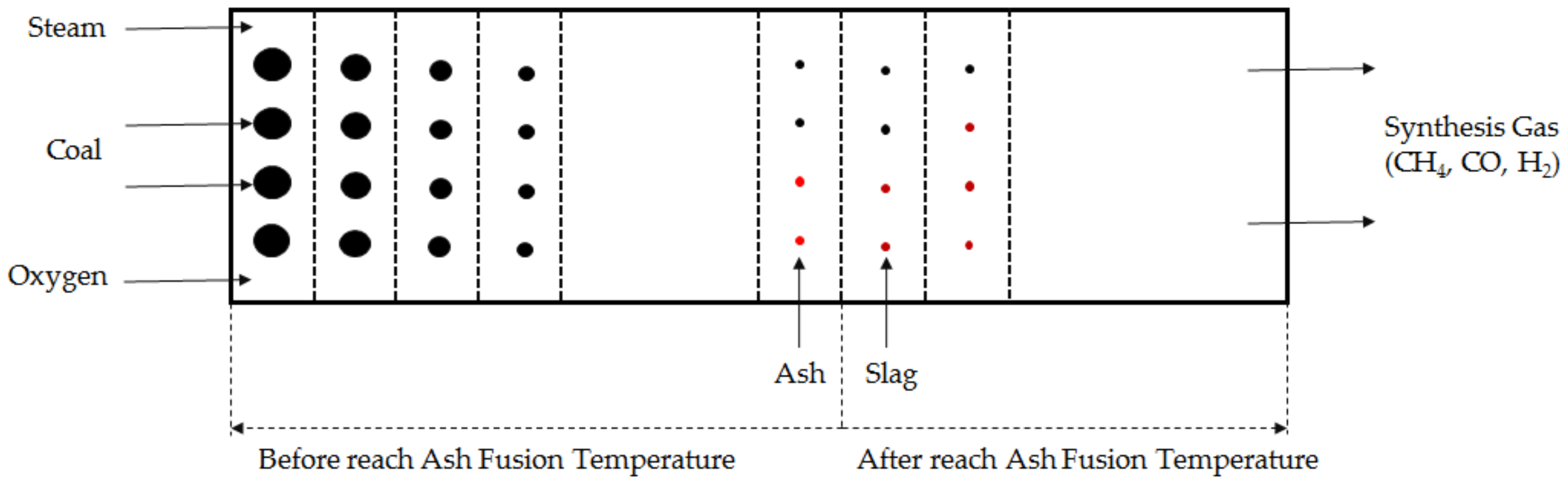
• The reactor consists of equally divided cells (Figure 1). The reaction rate depends on each cell’s conditions.
• Spherical coal particles react from the outer surface while moving through the cell from front to end. As the reaction of the coal progresses, the size of the particles decreases.
• All of the coal grains in the same cell are uniform.
• Ash changes to slag after temperature exceed an AFT.
• Ashes are inert.

2.2. Reaction Kinetics

The reaction type can be divided into a heterogeneous reaction and a homogeneous reaction. The heterogeneous reaction indicates that the coal particles react with the gas. Coal reacts with oxygen, carbon dioxide, steam, and hydrogen (

Table 2. Homogeneous and heterogeneous reaction list used in this study.

Reaction Type	Reaction	Description
Heterogeneous	$R_1:C_a{H}_b{O}_c{N}_d{S}_e{A}_f+\left(\frac{a}{{\varphi }^{*}}+\frac{b}{4}-\frac{c}{2}-\frac{e}{2}\right)O_2\to \left(\frac{2}{\varnothing }-1\right)aC{O}_2+2\left(1-\frac{1}{\varnothing }\right)aCO+\left(\frac{b}{2}-e\right)H_{2}O+e{H}_{2}S+\frac{d}{2}{N}_2+fA$	Coal↔O2
	$R_2:C_a{H}_b{O}_c{N}_d{S}_e{A}_f+aC{O}_2\to 2aCO+c{H}_{2}O+(\frac{b}{2}-c-e)H_2+e{H}_{2}S+\frac{d}{2}{N}_2+fA$	Coal↔CO2
	$R_3:C_a{H}_b{O}_c{N}_d{S}_e{A}_f+\left(a-c\right)H_{2}O\to aCO+\left(a+\frac{b}{2}-c-e\right)H_2+e{H}_{2}S+\frac{d}{2}{N}_2+fA$	Coal↔H2O
	$R_4:C_a{H}_b{O}_c{N}_d{S}_e{A}_f+\left(2a-\frac{b}{2}+c-e\right)H_2\to aC{H}_4+c{H}_{2}O+e{H}_{2}S+\frac{d}{2}{N}_2+fA$	Coal↔H2
Homogeneous	$R_5:CO+H_{2}O\leftrightarrow C{O}_2+H_2$	WGS
	$R_6:CO+\frac{1}{2}{O}_2\to C{O}_2$	CO oxidation

* φ is a function of absolute temperature T, and adjusts the ratio of complete and incomplete combustion. $\varnothing =\frac{2w+2}{w+2},w=2500·\exp \left(-\frac{6249}{T}\right)$. [4].

). The water gas shift reaction (WGS) and CO oxidation were considered as major reactions. The WGS reaction proceeds rapidly at a high temperature, and was therefore considered to be at equilibrium. CO oxidation was regarded as irreversible; as a consequence, gasification and combustion reaction could be expressed without dividing the reaction zone. Therefore, we solved reaction kinetics based on the single reaction zone; i.e., the six reaction schemes that are presented below were considered equally from the first cell to the last cells. The EFG does not produce much methane [19], so the methane-steam reforming reaction was not considered in this model.

To incorporate the coal components in reaction kinetics, the ultimate analysis was applied. The reaction kinetics (

Table 3. Reaction kinetics and parameters that were used in this study.

action Type	Reaction Rate (g/s)	k (g/(m2·atm·s))	Reference
Heterogeneous	$k_1\pi {d_c}^2{P}_{O_2}$	$6180·e^{(-\frac{10,233.9}{T})}$	[5,6]
	$k_2\pi {d_c}^2{P}_{C{O}_2}$	$198,100·e^{(-\frac{10,233.9}{T})}$
	$k_3\pi {d_c}^2{P}_{H_{2}O}$	$198,100·e^{(-\frac{10,233.9}{T})}$
	$k_4\pi {d_c}^2{P}_{H_2}$	$385·e^{(-\frac{17,451.7}{T})}$
Homogeneous	Equilibrium	Equilibrium Constant	Reference
	$\mathrm{K}=\frac{P_{C{O}_2}{P}_{H_2}}{P_{CO}{P}_{H_{2}O}}$	$-2.4198+0.003855·\mathrm{T}+\frac{2180.6}{T}$	[20]
	Reaction Rate (mole/s)	k (m3/(mole$·$s))	Reference
	$k_6{C}_{CO}{C}_{C{O}_2}$	$3.09·e^{(-\frac{11,199}{T})}$	[21]

) of coal used in this study was based on Hwang et al.’s work. One difference is that we have attempted to quantify ash. We introduce subscript f, which means that the ash component contained in 1 g of coal, and is the result of the proximate analysis. The subscripts a through e represent elements contained in 1g of coal. For heterogeneous reactions, the reaction rate of coal was proportional to both the surface area of the coal particles and the partial pressure of each gas. In homogeneous reactions, all of the gases were assumed to be ideal.

3. Solving Procedure

3.1. Mass Balance

For mass balance, only production and consumption due to the reaction were calculated. The kinetics of the coal reaction was based on one coal grain. The number of coal particles per unit volume came from the following Equation (1):

$$N_v=\frac{W_{c,0}}{m_c{v}_{c}A}$$

(1)

The four coal reactions caused the coal conversion when the coal particles passed through the unit cell. ∆z is unit cell length. The change of coal mass was calculated as

$$\Delta W_c=-N_v·A{\displaystyle \sum }_{i=1}^4{R}_i·\Delta z$$

(2)

Mass balance of the ash could be expressed in the same way as that of coal. The only difference is that the stoichiometric coefficients f are added. The stoichiometric coefficients that correspond to ashes were all equal to f (Equation (3)). For slag, the mass balance was not considered separately. When the temperature was higher than AFT, ash was regarded as slag.

$$\Delta W_a=-N_v·A{\displaystyle \sum }_{i=1}^4{R}_i·f·\Delta z$$

(3)

For gas mass balance, R₅ and R₆ were also included. R₆ is irreversible, so it was applied in the same manner as the heterogeneous reactions. α means the degree of deviation from equilibrium. To calculate α, we used Equation (4)

$$\mathrm{K}=\frac{\left(F_{C{O}_2}-\alpha \right)·\left(F_{H_2}-\alpha \right)}{\left(F_{CO}+\alpha \right)·\left(F_{H_{2}O}+\alpha \right)}$$

(4)

After converting this to an explicit form, we took a small root of the quadratic equation. The reason was that large roots make the mole flow negative.

Equation (5) is the mass balance of gases where ${\xi }_i$ is a stoichiometric coefficient for each component. Heterogeneous and homogeneous reactions were considered in different forms. The terms on the right side of the equation mean in order: (i) initial value; (ii) heterogeneous reactions; (iii) CO oxidation; and, (iv) each cell reaches equilibrium.

$$F_i=F_{i,0}-\left(N_v·A·\Delta z·{\displaystyle \sum }_{j=1}^4{\xi }_{i,j}·\frac{R_j}{M{W}_i}\right)+\left(R_5·{\xi }_{i,5}\right)\pm \alpha$$

(5)

3.2. Energy Balance

Heat flow of input and output and reaction enthalpy were considered equally in all cells. In some existing models [5,6,16,17], oxygen, steam, and coal temperature were set differently. When the temperatures of coal and gas are separately calculated, the temperature difference between them is generally ~10 K [22]. In this study, we simplified the problem by assuming that the gas temperature was the same as the coal temperature.

Coal residue is ash or slag depending on temperature condition (Figure 1). To consider ash melting, energy balance was calculated by dividing it into three cases. At temperature <AFT, Equation (6) was applied. It did not incorporate the fusion heat of ash.

$$\Delta \left\{\left(W_c·c_{p,c}+W_a·c_{p,a}+W_s·c_{p,s}+{\displaystyle \sum }_i{F}_i·c_{p,i}\right)\mathrm{T}\right\}=-N_v·A·{\displaystyle \sum }_{j=1}^6{R}_j·\Delta H_j-H_{loss}$$

(6)

Cells with temperature >AFT were considered using Equations (7) and (8). Equation (7) was applied only to the first cell, which has temperature >AFT. This equation calculates all of the latent heat of the accumulated ashes.

$$\Delta \left\{\left(W_c·c_{p,c}+W_a·c_{p,a}·W_s·c_{p,s}+{\displaystyle \sum }_i{F}_i·c_{p,i}\right)T\right\}=-N_v·A·{\displaystyle \sum }_{j=1}^6{R}_j·\Delta H_j+W_a·\Delta H_{ash}-H_{loss}$$

(7)

Equation (8) was applied to the remaining cells. It considers the heat of fusion of ash that occurs as it passes through each cell.

$$\Delta \left\{\left(W_c·c_{p,c}+W_a·c_{p,a}·W_s·c_{p,s}+{\displaystyle \sum }_i{F}_i·c_{p,i}\right)T\right\}=-N_v·A·{\displaystyle \sum }_{j=1}^6{R}_j·\Delta H_j+△W_a·\Delta H_{ash}-H_{loss}$$

(8)

Calculation of the heat loss must consider radiation, convection, and conduction. In addition, the thermal conductivity varies depending on the material of the refractory. If these cannot be reasonably estimated, the overall heat transfer coefficient will produce large errors. In a previous study, the heat transfer coefficient was indirectly estimated instead of calculating the heat loss [6,16,17]; the authors claimed that 30% of the reaction heat was lost to the outer wall, and that the corresponding calorific value is about 7–10% of the heating value of coal. However, heat losses typically considered in an EFG range from 1 to 4% [23,24]. This value is dependent on the gasifier scale. When compared with industrial gasifiers, pilot-scale gasifiers have higher heat losses. Therefore, we assumed a heat loss of 4%.

3.3. Solving Algorithm

The length of the gasifier was divided into 1650 cells (500 parts/m). Each cell was a system. Mass and energy balance were calculated sequentially. The computational algorithm was terminated when it reached the end of the reactor, and we obtain a sufficiently smooth curve in the simulation result. The information calculated in each cell was as follows:

• Information about coal: coal conversion, coal mass flow rate.
• Molar flow rate of product gas.
• Temperature profile.

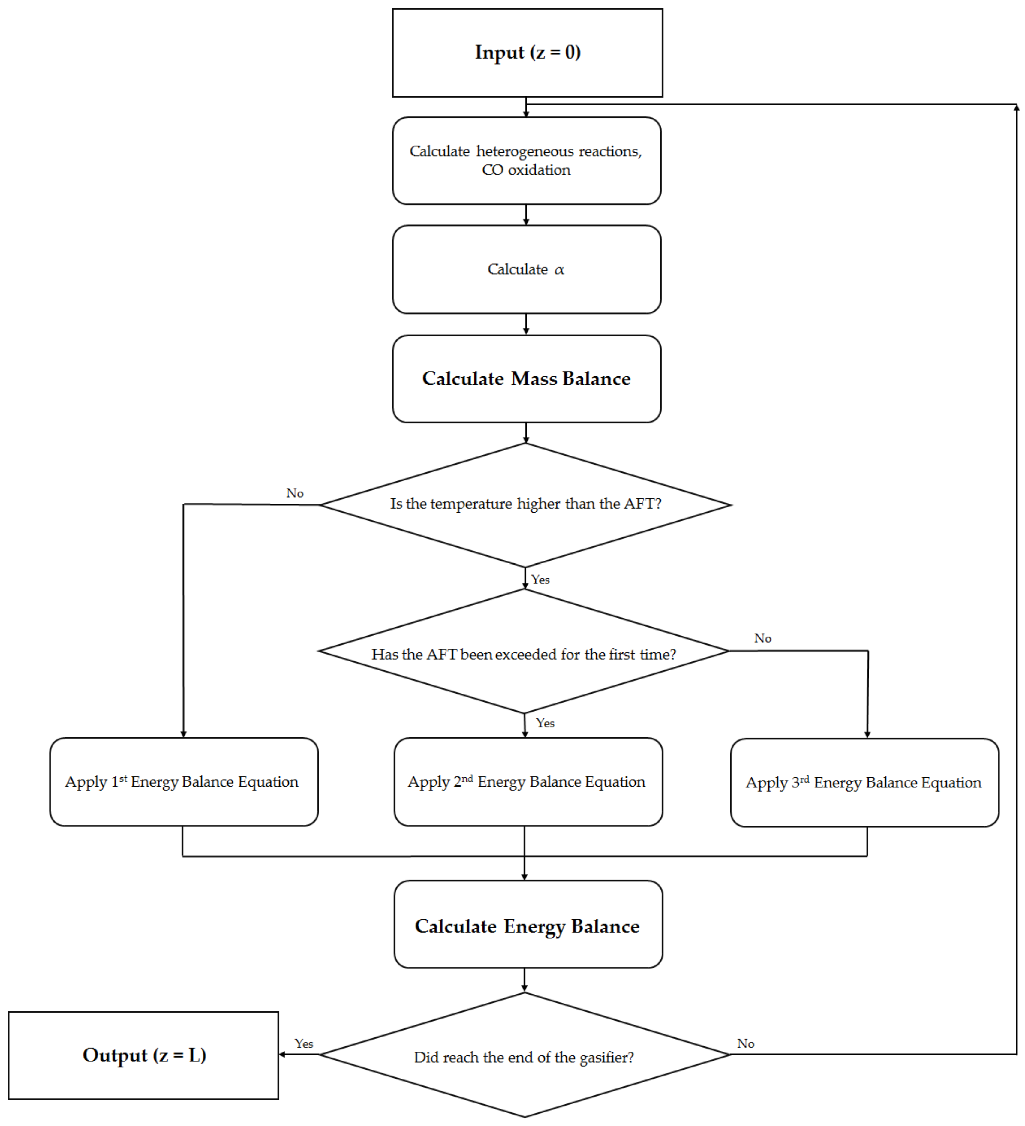
The proposed algorithm (Figure 2) was designed to apply the energy balance of three cases according to temperature. gPROMS simulation software (Process Systems Enterprise Ltd., London, UK) was used to perform the algorithm. The DASolver was applied; it could be used to solve differential equations in the steady state. Both the relative tolerance and absolute tolerance were fixed as 1.0 × 10⁻⁵.

4. Required Information for Simulation

4.1. Operating Variables and Reactor Size

Required inputs, including operating variables and particle sizes (

Table 4. Comparison of operating variables and gasifier size between this and previous studies.

Operating Variables	This Work	Wen	Govind
Coal feed rate (g/s)	50	75	77
Steam to coal ratio (-)	0.24	0.24	0.241
Oxygen to coal ratio (-)	0.86	0.86	0.86
Feed coal temperature (K)	900	900	505
Feed gas temperature (K)	900	900	697(H2O), 298(O2)
Gasifier pressure (MPa)	2.0	2.0	2.4
Gasifier wall temperature (K)	Not considered	2100–600(Z/L)	2100–600(Z/L)
Gasifier Size	This Work	Wen	Govind
Gasifier length (cm)	330	330	330
Inner diameter (cm)	152	152	152

), were those of the existing pilot gasifier. These results were compared with those of previous studies. The experimental conditions were presented in the work of Govind and Shah, which is the same as for their simulation conditions. Experimental information on the outer wall temperature of the gasifier was not provided. The existing model assumed that the temperature of the outer wall started at 2100 K, and then decreased linearly [16,17]. We indirectly estimated the amount of heat loss from the coal heating value, instead of assigning an initial outer wall temperature.

4.2. Coal Properties

This study considered Illinois no. 6 coal, which is the same type using previous modeling studies. The results (

Table 5. Element analysis (wt %), coal properties, and feed conditions that were used in this study.

Element	Measurement
C	74.05
H	6.25
O	1.32
N	0.71
S	1.77
Ash	15.33
Coal Properties	Assumed
Density (g/cm3)	1.80
Specific heat capacity (cal/(g·K))	0.45
Feed Conditions	Set
Feed particle size ($\mathsf{\mu }\mathrm{m}$. )	41
Velocity (cm/s)	50

) of coal elemental analysis were acquired from the EPRI [18]. Density and specific heat capacity of the coal were the same as in previous work [16,17]. We considered a smaller particle size (41 μm) of coal than did previous work, for two reasons. First, 41 μm is closer to the size of the particles that were used in the EFG in real industry; particularly, when entering a dry feed, the particle size is < 100 μm [25]. Second, the reaction of coal is directly related to particle size and kinetic parameters, so particle size is an important factor in kinetics. Therefore, the kinetic parameter and particle size must be taken from the same reference. We used the same kinetics parameters and the coal particle size as Hwang’s model [6].

4.3. Ash and Slag Properties

The EPRI provided only the coal analysis data; it does not provide information about ash. One of way to remedy this lack of information is to assume the ash component. However, the physical properties differ depending on the ash component. Calculate of thermal properties that consider its components is a difficult task. In some documents [26,27], a formula for predicting thermal properties according to the temperature have been proposed. However, they were out of the range of gasifier operating temperature.

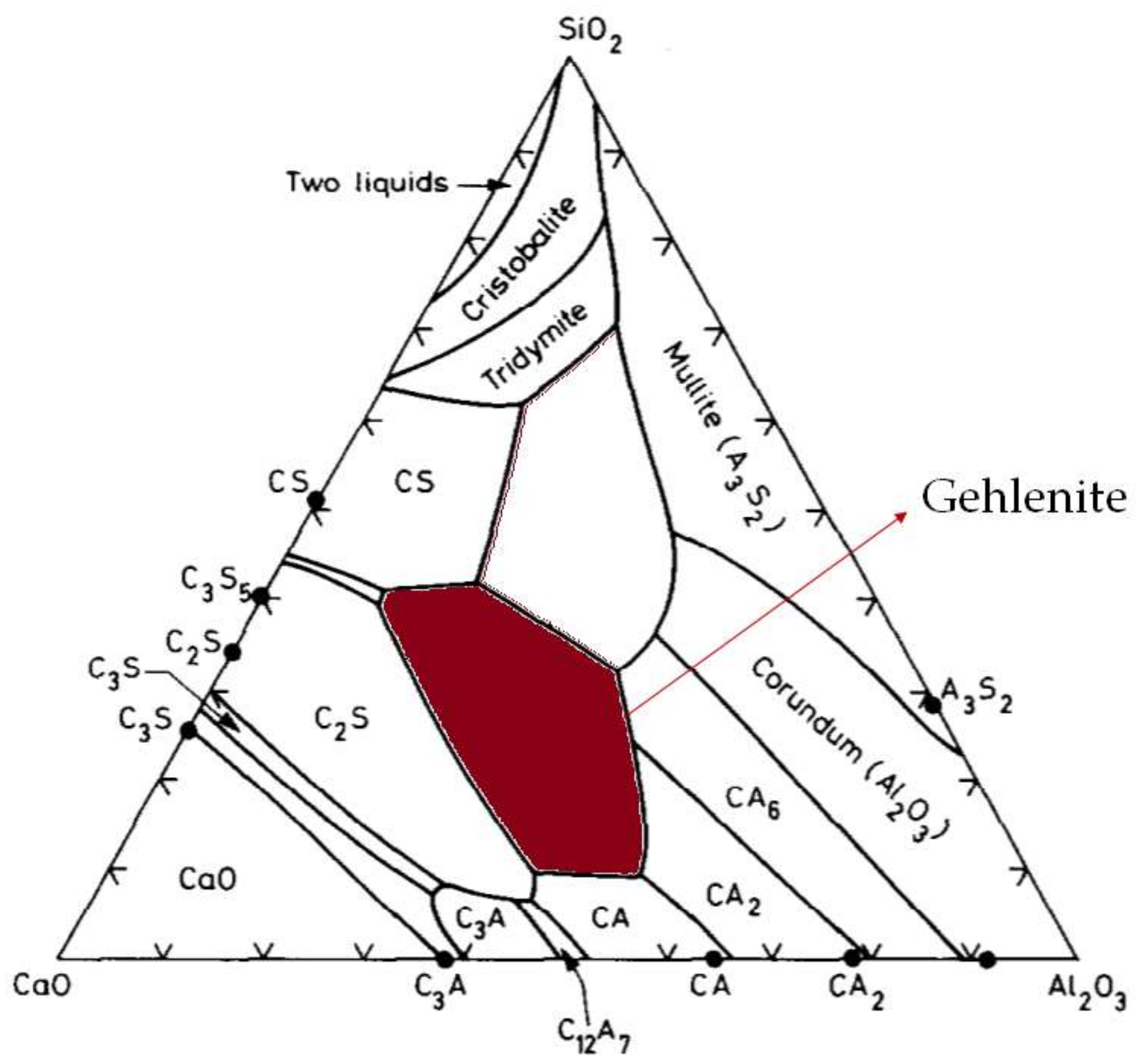
In this study, different approaches were used. Coal ashes are composed of minerals (Figure 3). About 70–90% of the constituents are CaO, Al₂O₃, and SiO₂. They also include such as Fe₂O₃ and MgO [28,29]. In this work, we adopt the thermal properties of gehlenite (Figure 3) to represent ash.

The properties (

Table 6. Thermal properties of ash and slag used in this study.

Thermal Properties	Value	Reference
Fusion heat of ash (J/g)	627.6	[30]
Ash fusion temperature (K)	1863	[30]
Specific heat capacity of ash (J/(g·K))	$-0.976+\mathrm{lnT}+\frac{279}{T}-\frac{1.094·{10}^5}{T^2}+\frac{1.169·{10}^7}{T^3}$	[31]
Specific heat capacity of slag (J/(g·K))	1.15	[32]

) of ash and slag used in this study were obtained from the literature because the ash was considered to be a well-known mineral, and its thermal properties were set accordingly.

5. Results and Discussion

5.1. Model Valdation

To validate the model, several main variables were selected: final coal conversion rate; major product gas composition at exit; and, the hydrogen-to-carbon monoxide ratio (H₂/CO). The results (

Table 7. Simulation results and comparison of previous models with experimental data (Dry based).

Major Variables	This Work	Wen [16]	Govind [17]	Experiment [17]
Conversion (%)	98.8	98.9	98.1	98.6
H2 (mole %)	38.6	39.8	40.0	39.1
CO (mole %)	57.7	56.6	55.5	57.6
H2/CO ratio	0.668	0.703	0.721	0.679
CO2 (mole %)	2.56	2.92	3.95	2.95

) of this simulation are presented together with the results of the previous researchers and experimental data. We did not arbitrarily adjust the kinetic parameters that were used in this study. We applied the same reactor size and operating conditions of the existing pilot gasifier. For this reason, results of this work were similar to results of previous studies. In addition, we considered the melting phenomenon of ash that was not considered in the existing one-dimensional (1-D) model and reduced the estimated heat loss in the previous model. As a result, the modeling results are improved.

5.2. Simulation Results

5.2.1. Coal Conversion

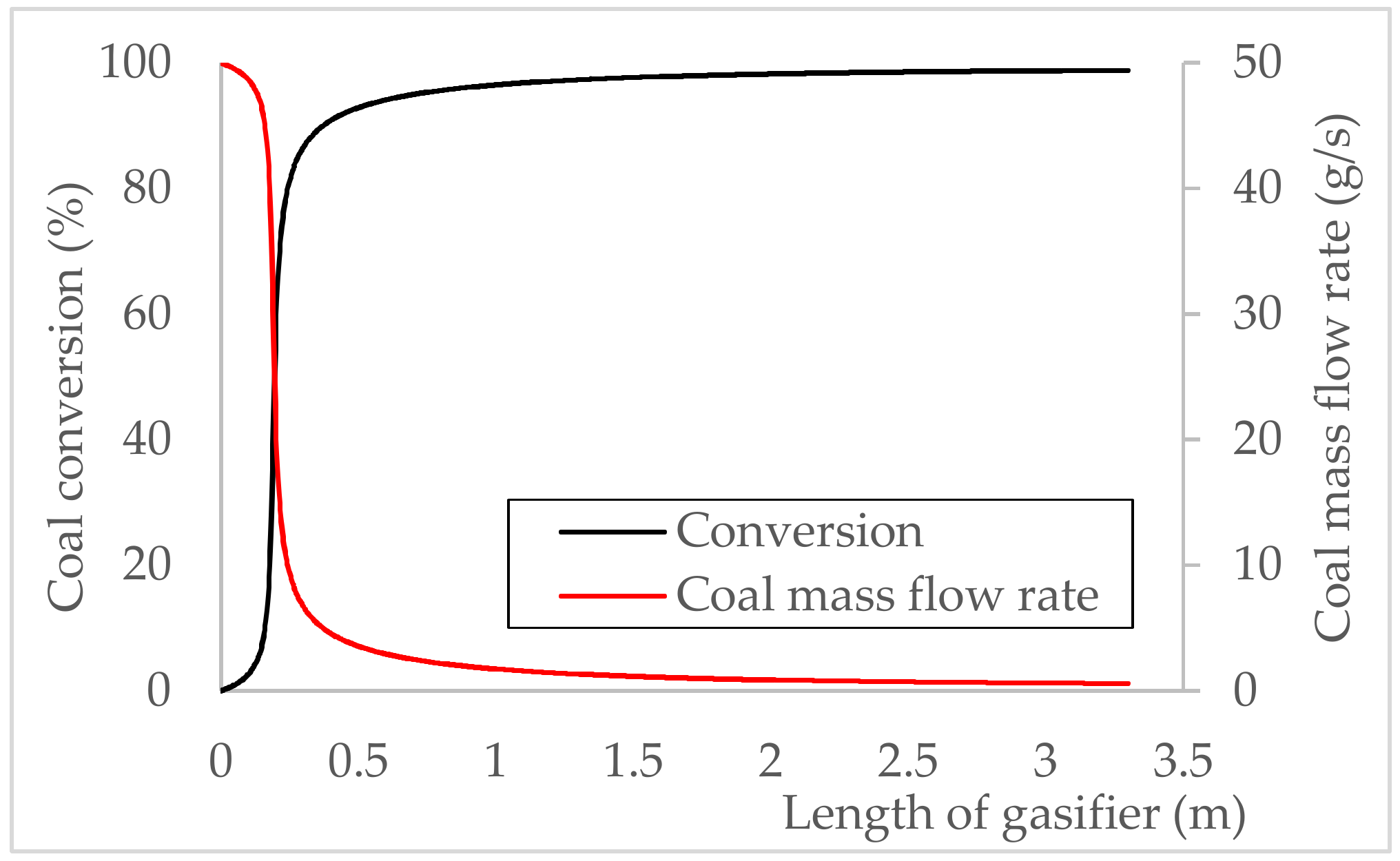
Most of the reaction proceeded rapidly at the front of the gasifier (Figure 4). Only 10% of coal was reacted at around 0.15 m of the gasifier, but 80% had reacted at 0.24 m. This increase occurred because the combustion reactions were accelerated. The reaction rate of coal decreased as the size of coal particles decreased. Especially after oxygen was completely consumed, the reaction rates were very slow. This trend is characteristic of typical EFGs; it is consistent with the results in past research [5,6,16]. The final coal conversion was 98.8%.

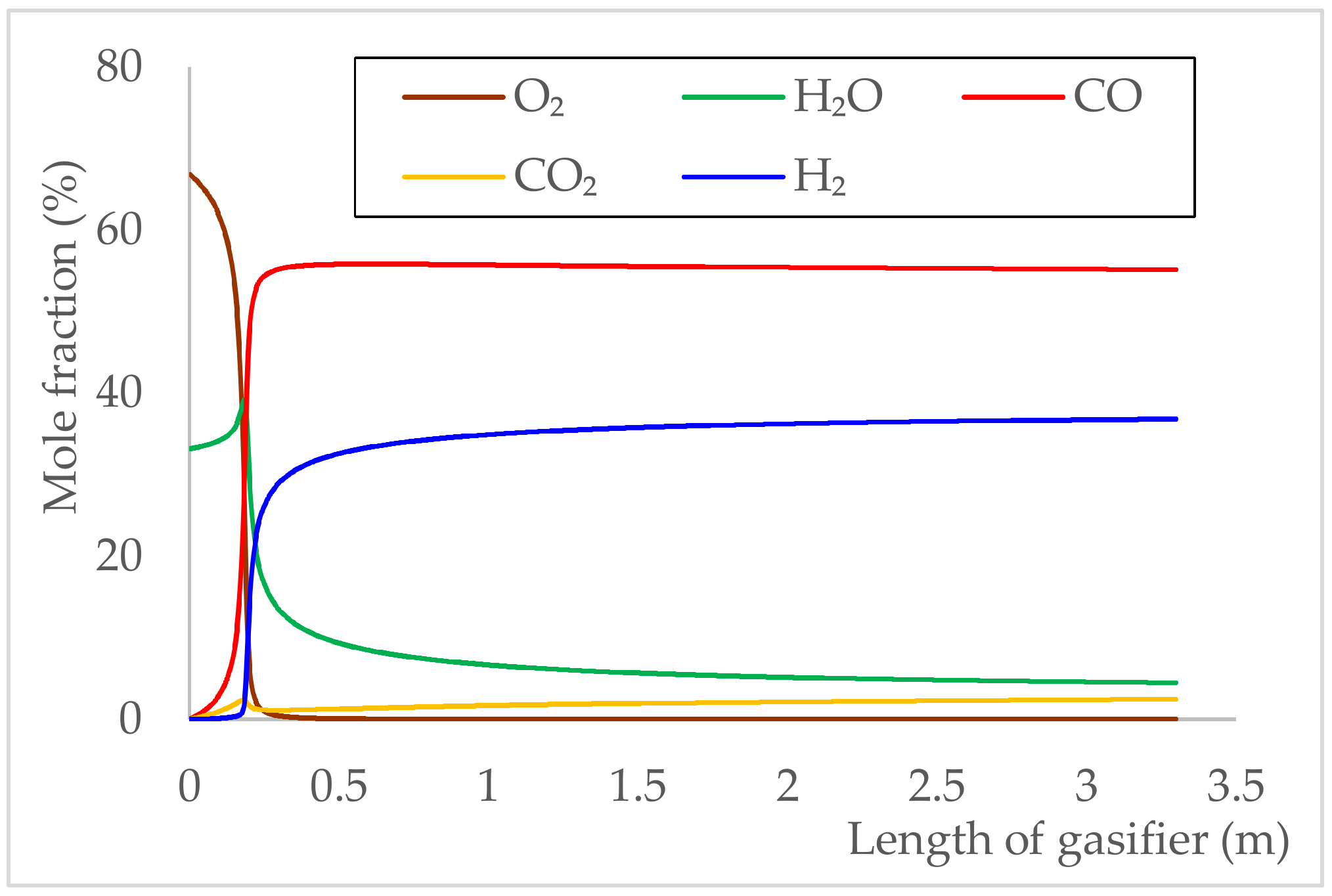
5.2.2. Gas Composition

The mole fractions of the major gases changed over the reactor length (Figure 5). Oxygen was abruptly consumed near 0.25 m; this change is the result of rapid combustion. Syngas was generated in an oxygen-free environment. Steam was slightly generated in the front of the gasifier; afterwards, the proportion of steam was controlled by WGS equilibrium. After all of the oxygen was consumed, the gas composition did not change significantly. CH₄, H₂S, and N₂ were < 1% of the product; they are not represented in Figure 5. Trends in the graph agreed with trends that were reported in previous research [5,6,16]. The exit gas consists mainly (mole fraction 98.9%) of carbon dioxide, hydrogen, steam, and carbon monoxide. All of these compositions are determined by WGS equilibrium, which is a function of temperature and is closely related to the outlet temperature of the gasifier. The attempt to calculate the temperature is the first step in predicting the composition of the gas, and this study is significant in that respect.

5.2.3. Temperature and Heat Flow

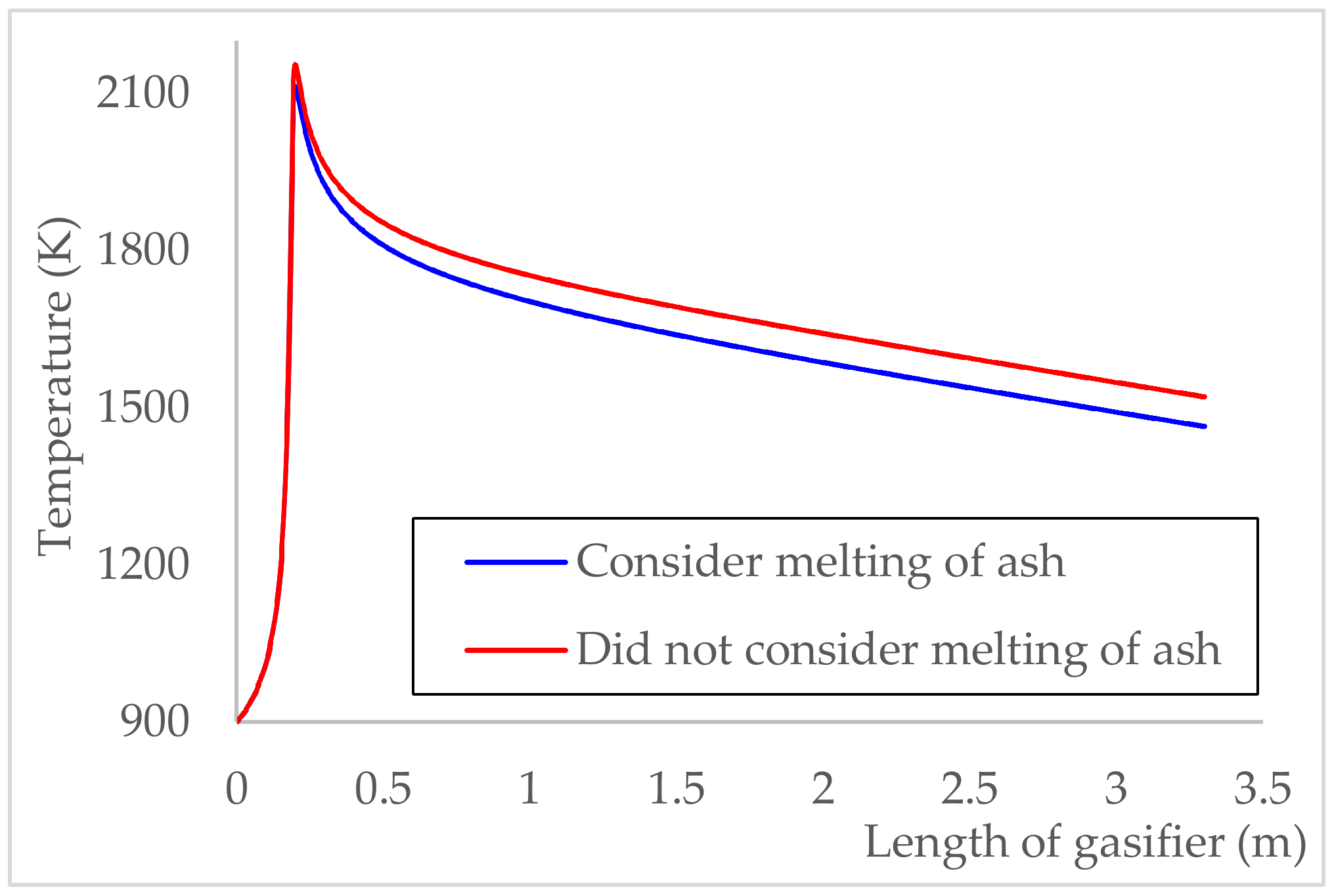
Simulations were used to calculate two temperature profiles (Figure 6). The heat balance of the first case (Figure 6, blue line) considered the sensible heat of the slag and the latent heat of the ash. The second case (Figure 6, red line) neglected these phenomena; both were set to 0. Below AFT, the temperatures of the two cases were the same, but the peak and outlet temperatures differed between the two cases. The same results were obtained in the temperature range below AFT; they are acceptable because the melting of ash had not yet been considered. The maximum temperature was calculated as 2112 K when sensible heat of the slag and the latent heat of the ash were considered, but 2155 K when they were neglected. The exit temperatures were 1464 K when the sensible heat of the slag and the latent heat of the ash were considered, and 1521 K when they were neglected; the difference between the two outlet temperatures was 57 K. The difference can be explained, as follows. The heat capacity of ash and slag is not taken into account in the system, and the corresponding energy was transferred to the gas, so the calculated temperature increased. Previous models have released heat to outside. EFGs generally use thick refractories. The assumption that a significant amount of heat escapes to the outside must be modified: these two temperature profiles show that the ash melting phenomenon must be considered when the internal temperature of the gasifier is calculated. This is a reasonable conclusion, given the fact that the internal peak temperature of the gasifier is higher than the AFT.

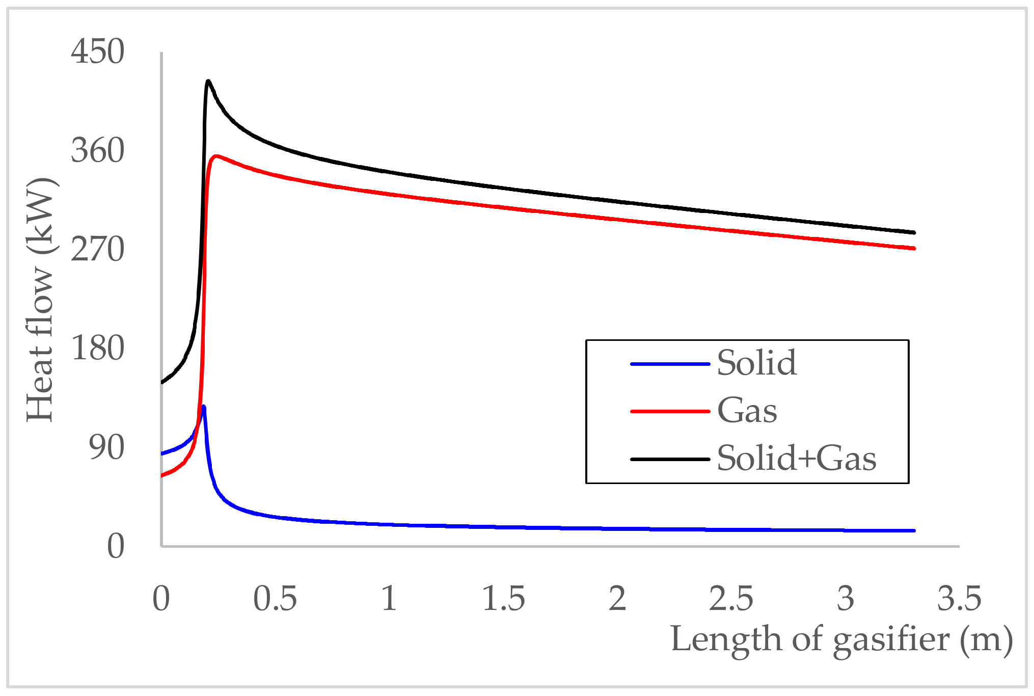
In this study, ash accounted for 15% of the mass of the coal and 7% of the total mass. The effect of sensible heat of slag is evident when the heat flows are divided into the solid and gas (Figure 7). Solids include coal, ash, and slag. After most of the reaction has proceeded, the solids are mainly in slag form. Especially at the exit condition, >99% of the solid was slag, which accounted for 5.0% of the total heat. In the coal that was used in this study, the ash was not negligible. As a result, our new attempt was meaningful. This phenomenon must be considered, especially for coal that has high ash content.

5.3. Consideration of Ash Melting Effect

The melting of ash has a similar effect on energy balance, as does heat loss from the outer wall. Because the ash melts and absorbs energy, the temperature of the system is lowered. In contrast, the loss to the outer wall lowers the temperature because heat escapes from of the system. These are different phenomena that occurred inside the gasifier, and were considered independently.

We quantitatively calculated the melting effect. This approach used the same method that was used to consider the heat loss. Based on the coal heating value, the latent heat of the ash and the sensible heat of the slag were calculated. The melting effect at the outlet was ~1%. This is not negligible given that heat loss is assumed to be 4% in this study. We calculated the melting effect at the exit as

$$\frac{SlagSensibleHeat+AshFusionHeat}{CoalHeatingValue\left(HHV\right)}=\frac{W_{s,L}·c_{P,s,L}·T_L+W_{a,L}·X_L·\Delta H_{ash}}{W_{c,0}·HHVofIllinoisNo.6}$$

(9)

In this way, we corrected the overestimate of heat loss that occurred in previous studies. In addition, we could explain some of the uncertainty of heat loss.

5.4. Applicability of High Ash Content Coal and Limitations

Coal containing a large amount of ash can be applied in the same manner. If information about the ash component is available, then it can be used to calculate the slag properties and incorporate thermal properties in the heat balance. When the ash content is high, modeling errors can be reduced by considering the fusion heat of ash and the sensible heat of the slag.

However, the reaction kinetic parameters that are cited in this study represent only coal combustion and gasification, so the model is only applicable to the entrained coal gasifier. In addition, lab-scale or pilot-scale data of other coal that has high ash content should be used to further assess applicability of this model.

6. Conclusions

This study suggests that a heat-balance model of an EFG must consider the effects of melting of ash. We attempted modeling based on kinetic models similar to those of previous researchers. Our proposed 1-D model is the only one that includes ash in the heat-balance and temperature-calculation algorithm. Gas production and coal conversion trends were similar to those of existing ones, and the results at the exit were mostly consistent with the experiments.

This result is meaningful in that it reflects actual phenomena occurring inside the EFG. Ash melts in any slagging-type gasifier. We can expect to calculate the internal temperature more accurately based on this study. These results can be used to guide the choice of design elements of EFG, such as material and thickness of the refractory wall.

One limitation of this model is that information on the ash component was not available. We used minerals to express ash components. This demerit must be eliminated. For further research, advanced modelling should use thermal properties based on ash analysis data. This model can be extended to account for radial direction temperature distribution.

References

- Phillips, J. Different types of gasifiers and their integration with gas turbines. In The Gas Turbine Handbook; 2006; Volume 1. Available online: https://www.netl.doe.gov/File%20Library/Research/Coal/energy%20systems/turbines/handbook/1-2-1.pdf (accessed on 2 January 2018).
- Guo, X.; Dai, Z.; Gong, X.; Chen, X.; Liu, H.; Wang, F.; Yu, Z. Performance of an entrained-flow gasification technology of pulverized coal in pilot-scale plant. Fuel Process. Technol. 2007, 88, 451–459. [Google Scholar] [CrossRef]
- Wang, T.; Stiegel, G.J. Integrated Gasification Combined Cycle (IGCC) Technologies; Woodhead Publishing: Cambridge, UK, 2016; ISBN 978-0-08-100185-1. [Google Scholar]
- Vamvuka, D.; Woodburn, E.T.; Senior, P.R. Modelling of an entrained flow coal gasifier. 2. Effect of operating conditions on reactor performance. Fuel 1995, 74, 1461–1465. [Google Scholar] [CrossRef]
- Vamvuka, D.; Woodburn, E.T.; Senior, P.R. Modelling of an entrained flow coal gasifier. 1. Development of the model and general predictions. Fuel 1995, 74, 1452–1460. [Google Scholar] [CrossRef]
- Hwang, M.; Song, E.; Song, J. One-Dimensional Modeling of an Entrained Coal Gasification Process Using Kinetic Parameters. Energies 2016, 9, 99. [Google Scholar] [CrossRef]
- Bhatia, S.K.; Perlmutter, D.D. A random pore model for fluid-solid reactions: II. Diffusion and transport effects. AIChE J. 1981, 27, 247–254. [Google Scholar] [CrossRef]
- Ishida, M.; Wen, C.Y. Comparison of kinetic and diffusional models for solid-gas reactions. AIChE J. 1968, 14, 311–317. [Google Scholar] [CrossRef]
- Sadhukhan, A.K.; Gupta, P.; Saha, R.K. Modelling of combustion characteristics of high ash coal char particles at high pressure: Shrinking reactive core model. Fuel 2010, 89, 162–169. [Google Scholar] [CrossRef]
- Gupta, P.; Sadhukhan, A.K.; Saha, R.K. Analysis of the combustion reaction of carbon and lignite char with ignition and extinction phenomena: Shrinking sphere model. Int. J. Chem. Kinet. 2007, 39, 307–319. [Google Scholar] [CrossRef]
- Kong, X.; Zhong, W.; Du, W.; Qian, F. Three Stage Equilibrium Model for Coal Gasification in Entrained Flow Gasifiers Based on Aspen Plus. Chin. J. Chem. Eng. 2013, 21, 79–84. [Google Scholar] [CrossRef]
- Biagini, E.; Bardi, A.; Pannocchia, G.; Tognotti, L. Development of an Entrained Flow Gasifier Model for Process Optimization Study. Ind. Eng. Chem. Res. 2009, 48, 9028–9033. [Google Scholar] [CrossRef]
- Chen, C.; Horio, M.; Kojima, T. Numerical simulation of entrained flow coal gasifiers. Part I: Modeling of coal gasification in an entrained flow gasifier. Chem. Eng. Sci. 2000, 55, 3861–3874. [Google Scholar] [CrossRef]
- Eri, Q.; Wu, W.; Zhao, X. Numerical Investigation of the Air-Steam Biomass Gasification Process Based on Thermodynamic Equilibrium Model. Energies 2017, 10, 2163. [Google Scholar] [CrossRef]
- Liu, X.; Wei, J.; Huo, W.; Yu, G. Gasification under CO2–Steam Mixture: Kinetic Model Study Based on Shared Active Sites. Energies 2017, 10, 1890. [Google Scholar] [CrossRef]
- Wen, C.Y.; Chaung, T.Z. Entrainment Coal Gasification Modeling. Ind. Eng. Chem. Process Des. Dev. 1979, 18, 684–695. [Google Scholar] [CrossRef]
- Govind, R.; Shah, J. Modeling and simulation of an entrained flow coal gasifier. AIChE J. 1984, 30, 79–92. [Google Scholar] [CrossRef]
- Robin, A.M. Hydrogen Production from Coal Liquefaction Residues; Final Report; Montebello Research Lab, Texaco, Inc.: Montebello, CA, USA, 1976. [Google Scholar]
- Basu, P. Biomass Gasification and Pyrolysis: Practical Design and Theory; Academic Press: New York, NY, USA, 2010; ISBN 978-0-08-096162-0. [Google Scholar]
- Callaghan, C.A. Kinetics and Catalysis of the Water-Gas-Shift Reaction: A Microkinetic and Graph Theoretic Approach. Ph.D Dissertation, Worcester Polytechnic Institute, Worcester, MA, USA, 2006. [Google Scholar]
- Deng, Z.; Xiao, R.; Jin, B.; Huang, H.; Shen, L.; Song, Q.; Li, Q. Computational Fluid Dynamics Modeling of Coal Gasification in a Pressurized Spout-Fluid Bed. Energy Fuels 2008, 22, 1560–1569. [Google Scholar] [CrossRef]
- Breault, R.W. Gasification Processes Old and New: A Basic Review of the Major Technologies. Energies 2010, 3, 216–240. [Google Scholar] [CrossRef]
- Gazzani, M.; Manzolini, G.; Macchi, E.; Ghoniem, A.F. Reduced order modeling of the Shell–Prenflo entrained flow gasifier. Fuel 2013, 104, 822–837. [Google Scholar] [CrossRef]
- Tremel, A.; Becherer, D.; Fendt, S.; Gaderer, M.; Spliethoff, H. Performance of entrained flow and fluidised bed biomass gasifiers on different scales. Energy Convers. Manag. 2013, 69, 95–106. [Google Scholar] [CrossRef]
- Krishnamoorthy, V.; Pisupati, S.V. A Critical Review of Mineral Matter Related Issues during Gasification of Coal in Fixed, Fluidized, and Entrained Flow Gasifiers. Energies 2015, 8, 10430–10463. [Google Scholar] [CrossRef]
- Richardson, M.J. The specific heats of coals, cokes and their ashes. Fuel 1993, 72, 1047–1053. [Google Scholar] [CrossRef]
- Rezaei, H.R.; Gupta, R.P.; Bryant, G.W.; Hart, J.T.; Liu, G.S.; Bailey, C.W.; Wall, T.F.; Miyamae, S.; Makino, K.; Endo, Y. Thermal conductivity of coal ash and slags and models used. Fuel 2000, 79, 1697–1710. [Google Scholar] [CrossRef]
- Mills, K.C.; Rhine, J.M. The measurement and estimation of the physical properties of slags formed during coal gasification: 1. Properties relevant to fluid flow. Fuel 1989, 68, 193–200. [Google Scholar] [CrossRef]
- Blissett, R.S.; Rowson, N.A. A review of the multi-component utilisation of coal fly ash. Fuel 2012, 97, 1–23. [Google Scholar] [CrossRef]
- Žigo, O.; Adamkovičová, K.; Kosa, L.; Nerád, I.; Proks, I. Determination of the heat of fusion of 2CaOAl2O3 SiO2 (gehlenite). Chem. Pap. 1987, 41, 171–181. [Google Scholar]
- Richet, P.; Fiquet, G. High-Temperature Heat Capacity and Premelting of Minerals in the System MgO-CaO-Al2O3-SiO2. J. Geophys. Res. 1991, 96, 445–456. [Google Scholar] [CrossRef]
- Berman, R.G.; Brown, T.H. Heat capacity of minerals in the system Na2O-K2O-CaO-MgO-FeO-Fe2O3-Al2O3SiO2-TiO2-H2O-CO2: Representation, estimation, and high temperature extrapolation. Contrib. Mineral. Petrol. 1985, 89, 168–183. [Google Scholar] [CrossRef]
Figure 1.
Gasifier internal scheme that considers melting of ash. Red dot: ash; brown dot: slag.
Figure 2.
Algorithm that includes the melting of ash.
Figure 3.
Ternary phase diagram of Al2O3-CaO-SiO2. Brown: gehlenite.
Figure 4.
The profile of the coal conversion and coal mass flow rate.
Figure 5.
The profile of the major product gas mole fraction.
Figure 6.
Differences in temperature profile depending on whether melting of ash is considered or not.
Figure 7.
Heat flow of solid and gas.