Value of Residential Investment in Photovoltaics and Batteries in Networks: A Techno-Economic Analysis

Abstract

Australia has one of the highest rates of residential photovoltaics penetration in the world. The willingness of households to privately invest in energy infrastructure, and the maturing of battery technology, provides significant scope for more efficient energy networks. The purpose of this paper is to evaluate the scope for promoting distributed generation and storage from within existing network spending. In this paper, a techno-economic analysis is conducted to evaluate the economic impacts on networks of private investment in energy infrastructure. A highly granular probabilistic model of households within a test area was developed and an economic evaluation of both household and network sectors performed. Results of this paper show that PV only installations carry the greatest private return and, at current battery prices, the economics of combined PV and battery systems is marginal. However, when network benefits arising from reducing residential evening peaks, improved reliability, and losses avoided are considered, this can more than compensate for private economic losses. The main conclusion of this paper is that there is significant scope for network benefits in retrofitting existing housing stock through the incentivization of a policy of a more rapid adoption of distributed generation and residential battery storage.

1. Introduction

Policy responses to climate change are transforming energy networks with the rise in distributed renewable energy generation. In Australia, policy measures to incentivize the take-up of residential photovoltaics (PV) coincided with a time of network driven electricity price rises, with average household bills increasing by two-thirds from 2007 to 2013 [1]. This has spurred one of the highest rates of solar penetration in the world with over 1.79 million, or 17% of, households installing PV. Nationally, households have installed 5.3 GW of PV generation, as of December 2016, which is forecast to rise to 12.55 GW by 2037 [2]. In many regions, over 40% of residential dwellings have PV installed [3].

This extent of PV adoption has challenged the operational and planning processes of distribution network service providers (DNSP) due to both the change in household demand profiles and voltage regulation issues during high generation periods.

The impact of PV generation on reducing household energy demand, combined with an increase in appliance and building efficiencies, has let to flat or declining annual aggregate volumes of energy served since 2009 [2]. Compounding the issue of declining or static energy volumes is the continued growth of system peak demand, particularly in New South Wales (NSW) and Queensland, reaching a record in Queensland of 9357 MW in January 2017 [4].

To date, energy volumes served have been the primary basis for the recovery of network costs by DNSPs. With distribution costs in Australia accounting for 37% of the retail bill, and transmission a further 8% [2]. The current 2014-19 Australian Energy Regulator (AER) determination of $6576.4 M (regulated five-year spending plan) for the NSW DNSP Ausgrid, considered in this study, represents cost recovery of 48.7% capital expenditure (capex), 30.3% operational expenditure (opex), and 21% regulated return including the return of capital (depreciation) and return on capital [5]. Further, under all current DNSP determinations in the National Energy Market (NEM) total approved distribution spending is $36,637 M of which $19,301 M is capex [6]. This is illustrative of the high proportion of capex value that could be accessed by displacing traditional network spending, or diverting to householders in the form of incentives to drive a rapid transformation of electricity networks.

Changing load conditions and a lack of policy certainty regarding carbon reduction strategies have found existing network cost recovery methods slow to adapt [7]. One effect of the reduction in energy served has been to exacerbate network driven price rises as the costs of the network are recovered on a smaller base. This effect has been referred to as the network ‘death-spiral’ [8], where high network prices resulting from network investment have incentivized households to install PV to manage their energy use. This in turn, by shrinking the base, results in further price increases and so on, raising the threat of leaving DNSPs with stranded assets in the absence of more efficient pricing strategies. This also presents social equity issues for those unable to afford the upfront investment in renewable generation to manage their price exposure.

The intermittency of PV generation has also posed network management challenges to DNSPs. The variability of PV generation is most felt in its impact on forecasting, frequency, and voltage variation. Studies have shown that LV networks can reach up to 20–30% penetration before there are significant network voltage quality issues [9,10,11].

The rapid technological advancement of battery energy storage systems (BESS) [12,13], has presented an opportunity to address the technical and economic challenges in transitioning to higher levels of distributed generation (DG) in electricity networks [14,15,16]. BESS can be used to meet demand through stored energy as well as managing PV generation intermittency and maintaining network voltage and frequency within allowable limits [17,18,19]. Further, BESS can be used to improve the efficiency of the network by displacing peak demand driven network spending [20,21,22].

If the rate of BESS adoption follows a similar pattern to that of PV, accelerated by continued reductions in capital costs, it will change the characteristics of the network itself [23]. Indeed in 2017 as a greater range of residential battery products came to market there was a more than doubling of installed PV and BESS systems as shown in

Table 1. Installed capacity of PV with battery storage (no. of systems).

Year	ACT	NSW	NT	QLD	SA	TAS	VIC	WA	Total
2014	8	208	3	129	34	5	137	169	693
2015	3	133	1	186	21	6	163	24	537
2016	105	667	6	330	130	18	240	70	1566
2017	162	1604	16	684	420	87	598	192	3763
Total	278	2612	26	1329	605	116	1138	455	6559

Source: Clean Energy Regulator [24].

.

Households combining PV and BESS have moved into the realm of the ‘prosumer’ where they gain the ability to both produce energy and manage their energy use [1,25,26]. This will upturn the current ‘price-taker’ relationship between households and DNSPs, and how this is managed in terms of collaboration in reaching greater levels of network efficiency and renewable generation will be crucial in transitioning energy networks to a low-carbon future.

Combined with advanced metering the rise of the ‘prosumer’ will enable greater freedom for households to aggregate into ‘smart grids’ or other arrangements of aggregation which provides further options for greater network efficiencies through the pooling of generation and storage both within and across regions [27,28].

Traditional approaches of volume-based cost recovery are becoming increasingly inefficient, hence innovative approaches to cost recovery, whilst encouraging innovation and network efficiency, are required. Studies have shown that the development of new network pricing methods are hampered by the lack of information to form truly cost-reflective pricing [7,29,30]. Building on their work, a thorough evaluation of the economic drivers of all network participants must be undertaken to provide the optimum balance between the objectives of increasing network efficiency and the decarbonizing of energy systems.

Prior research into the economics of DG at the household level, and increasingly the addition of BESS, primarily has focused on the private costs to investors and the gains arising through self-consumption, peak shaving, and energy export [31,32]. The price of peak energy under time of use (ToU) was an important factor in determining value, however, BESS costs were still found to be the primary determinant of profitability in South African pricing conditions [33]. Similarly, a publication found that with domestic BESS prices in 2014, under German electricity pricing conditions, that the gains from incorporating BESS with PV justified the investment in BESS [34]. Further a study analyzing a university building in Bologna, Italy, found that the incorporation of BESS and PV resulted in savings of 24.5% on grid electricity prices [35]. In Australia a paper found that there was high probability of economic gains based on BESS costs of $500/kWh, 14 kWh sized battery with 75% efficiency [36]. However, a more recent paper from Italy found that the economics of PV and BESS are justified only when there is a significant increase in self-consumption [37]. A recent paper compared residential business cases against that of a large-scale project with consideration of gravity storage as an option, it found that in residential cases batteries were uneconomical [38]. However, the authors did not ascribe any value from the deferment of network upgrades to actions taken by households.

Where the economic perspective of DNSPs has been evaluated, whether in evaluating microgrids [39,40] or mitigating forecasting uncertainty as in [19], the most commonly identified benefit is deferring network spending [41,42], and to a lesser extent the provision of ancillary services as the primary network benefits. The deferral of network spending has through various studies has ranged from AUD$1200 [43] per kVA displaced, to $1500 AUD/kVa in 2009$ [41], a more recent figure of $810 per kVa (2012 AUD$) has been obtained from the AEMC Power of Choice report for the Ausgrid Network area [44]. However, in these studies into benefits of DG they have not considered residential renewable energy and storage as the source of supply.

To date, despite the wealth of papers analyzing household economics of photovoltaics and storage, there are few studies that seek to provide an integrated household and network economics impact model. In the literature there is clearly a divide between the household sector perspective and that of the network operators. The predominant network impact considered has been voltage and frequency stability arising from a surplus of household PV generation. This is an important consideration; however, it is the view of the authors that this leaves much of the changing nature of energy systems and the impact of prosumers underexamined.

Without a clear understanding of the full range of impacts on network capital spending, customer reliability and the reduction of losses there is a significant gap in the ability to evaluate the impact of household energy investment decisions. Given the high proportion of network costs in energy prices, a clear view of the potential network benefits arising from private household energy investments will allow the identification of network spending efficiencies and inform the scope for, and incentivization of, greater levels of household renewable generation. Such an understanding will assist in addressing the resistance of network operators to further incorporation of DG. Whether based on risk aversion or industry culture, in cases of push-back on the spread of DG as explored in a paper by Simpson [45], through increasing of cost and complexity of connection agreements, a clear understanding of wider economic benefits can help address this resistance.

In order to provide this novel perspective, the purpose of this research is to develop a probabilistic techno-economic model that integrates a highly-granular household energy system model combined with an economic analysis of network sector impacts. Stochasticity in input variables will be addressed by using a Monte Carlo (MC) simulation. MC modelling combined with Life Cycle Cost (LCC) is a common methodology for incorporating uncertainty across a range of scenarios by random sampling using probability distributions [46,47,48].

This paper is organized as follows, Section 2 presents the methods used to perform the simulations and economic analysis, Section 3 presents the results of the modelling, and Section 4 presents the conclusions of the analyses.

2. Methods

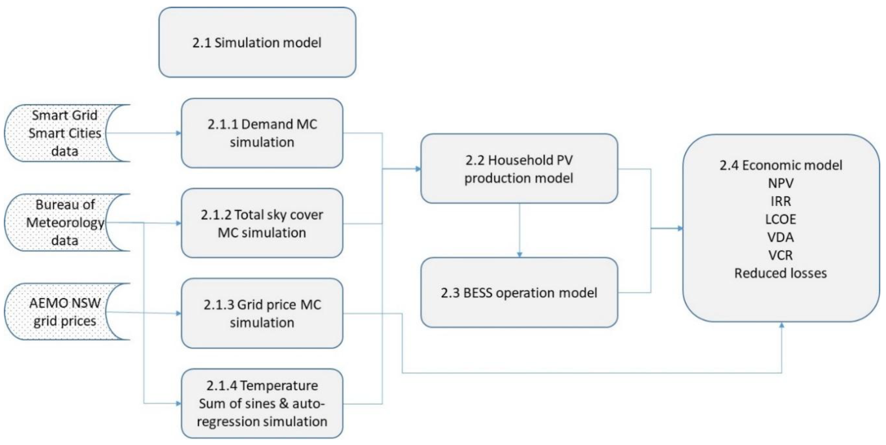
The techno-economic model will be comprised of a series of modules constructed in the MATLAB (2016a, Mathworks Inc., Natick, MA, USA) environment. It will be comprised of: simulation, household PV production, BESS operation, and economic modules as shown in Figure 1.

2.1. Simulation Model

Due to the highly variable nature of the input parameters, such as household demand, temperature, total sky cover (TCS), and global irradiance simulation methodologies have been selected to reflect underlying seasonal patterns as well as incorporating short-term stochasticity.

2.1.1. Demand Simulation Methodology

Under the NSW Smart Grid Smart City Project (SGSC) [49] the first commercial scale smart grid roll-out in Australia 2010–2014, energy use data was collected at the half hourly level for over 78,000 households across the Sydney and Newcastle regions in Australia. It provides a rich data source of demographic information as well as energy infrastructure characteristics of each household. To ensure that the selected household energy profiles are purely electricity focused those households that utilized gas heating, were without demographic data, or did not have one full year of meter readings were excluded.

A household’s demand profile is based upon a range of demographic, seasonal, weather and consumer behaviors and so is highly stochastic in nature. To derive a simulation profile that preserves the seasonal shape whilst preserving the intra-period stochasticity historical energy use data was analyzed at the half-hourly period. The simulation was performed at each half-hourly time step with demand as a normally distributed variable using historically derived input parameters for each period.

2.1.2. Total Sky Cover Simulation

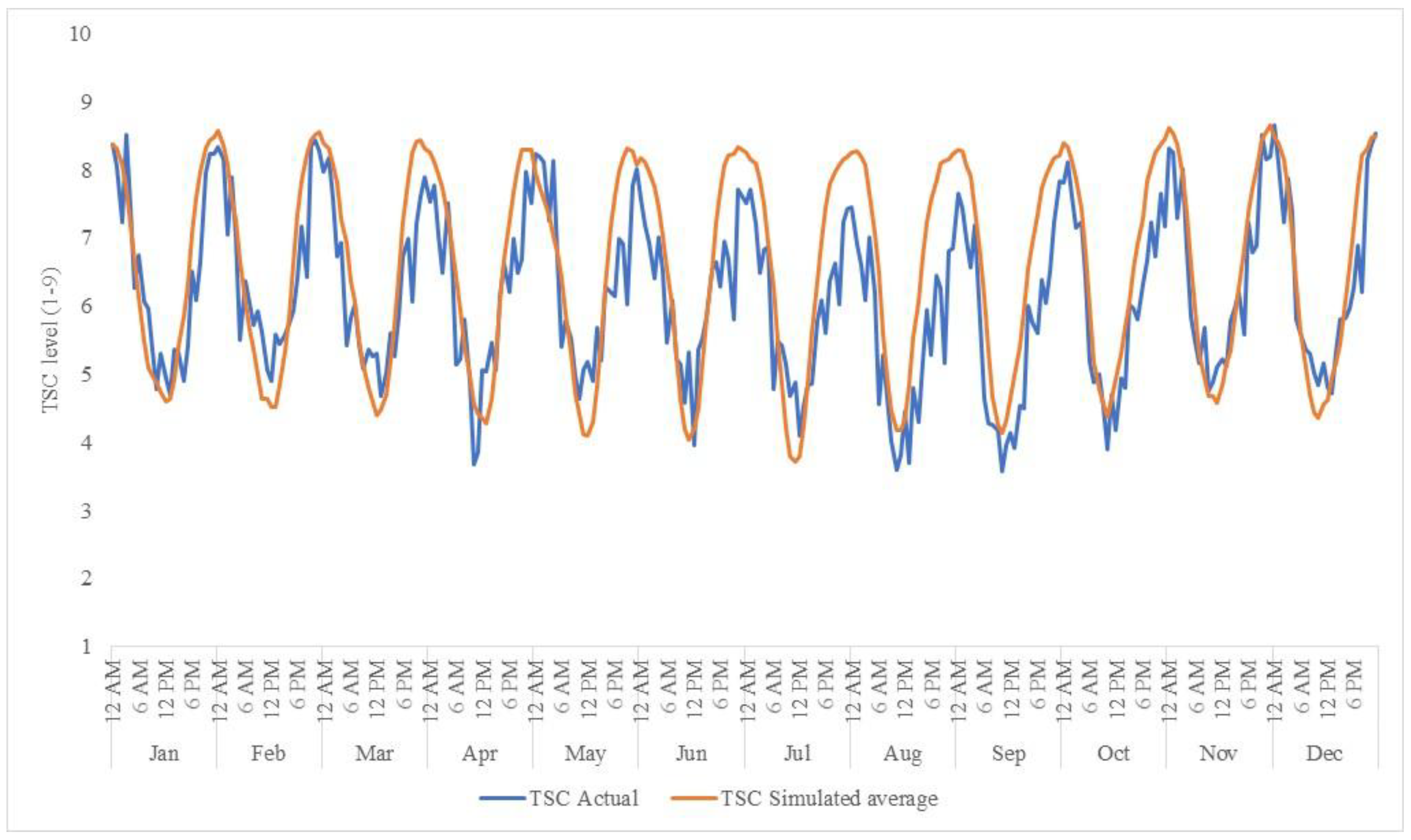
TSC simulation was based on analysis of Bureau of Meteorology (BOM) data, Williamtown station ID: 94776, of the years 2010–2012. Similarly, to Section 2.1.1 analysis was made at the half-hourly level and then TSC simulated as a normally distributed variable at each timestep using historically derived input parameters for each period.

2.1.3. Grid Price Simulation

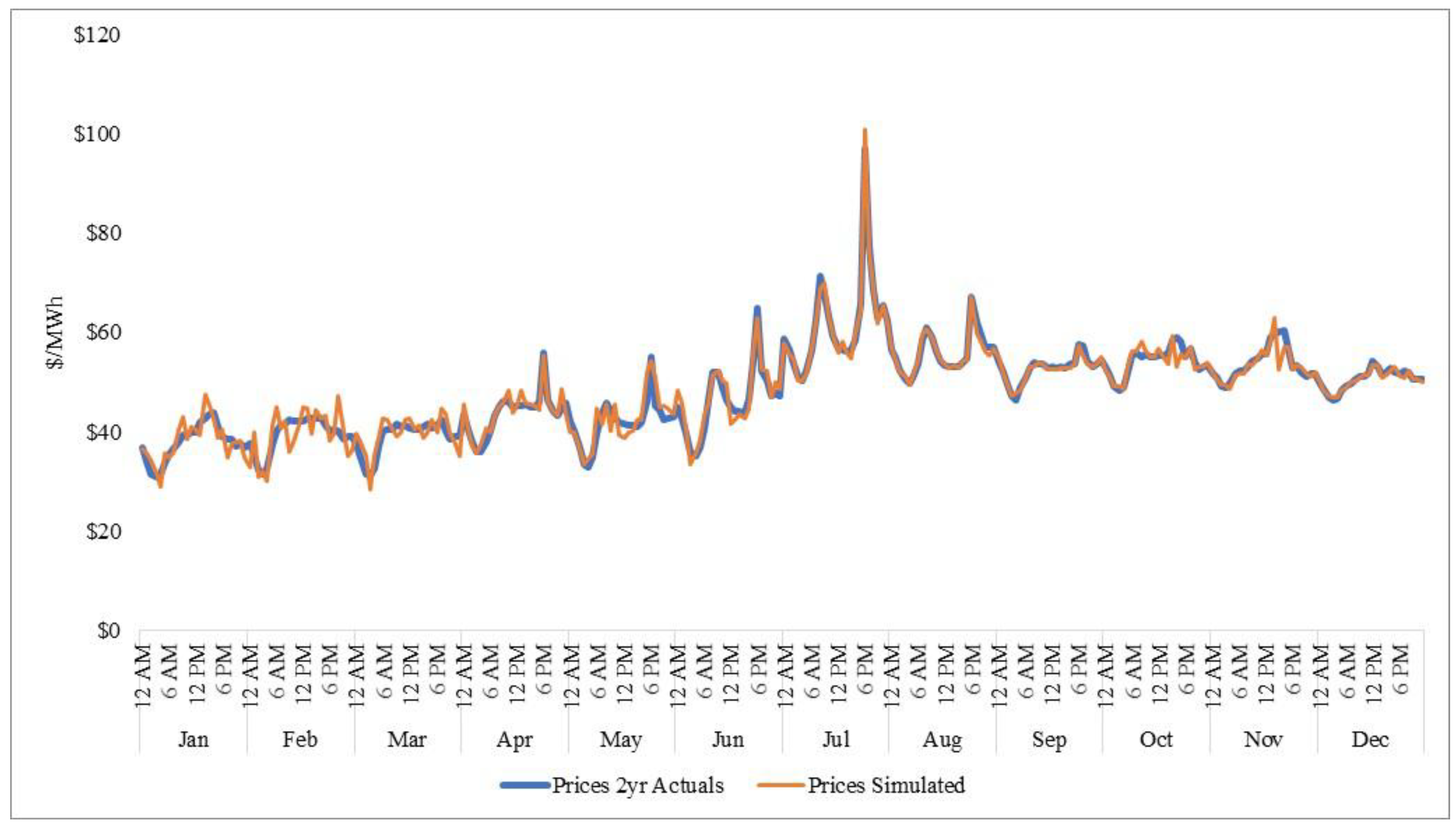
The grid price model was based on analysis of the years 2012–2013 for NSW network prices sourced from the Australian Energy Market Operator (AEMO), to derive the input parameters for each half hourly period for simulation. A simplified method for price forecasting, based on historical shape as opposed to market supply and demand modelling, has been selected so to preserve the seasonal shape, provides sufficient short-term variation and reduces complexity in the resulting model.

2.1.4. Temperature Simulation

For the purposes of simulating the seasonally variable inputs to the household model a methodology was chosen that can capture both the deterministic structural, or seasonal, components of the temperature as well as its stochastic nature [50].

• The deterministic or seasonal component is modelled with a sum of sines model that reflects the cyclical nature of the underlying structure of variables [51].

  $$\mathrm{y}={{\displaystyle \sum }}_{\mathrm{i}=1}^{\mathrm{n}}{\mathrm{a}}_{\mathrm{i}}\sin ({\mathrm{b}}_{\mathrm{i}}\mathrm{x}+{\mathrm{c}}_{\mathrm{i}})$$

  (1)

  where a = amplitude, b = frequency, and c = phase constant for each sine wave term. One year of historical data for each of the variables is analyzed and the parameters of the respective sum of sine models are estimated using the curve fitting function in MATLAB [52]. The serial correlation of the residuals is analyzed through use of the partial autocorrelation function [51].
• The stochastic component of the model is determined by using an auto-regressive model with seasonal lags, lags derived from the partial autocorrelation function. The resulting residuals of the regression are again analyzed for serial correlation, and a distribution is fit to the residuals. The resulting model is then simulated, outliers removed, and the results compared to historical data.

2.2. Household PV Production Model

PV production will be based on standard solar irradiance calculation and PV production methodologies [53], combined with analysis of historical BOM global irradiance and TSC data.

The simulation model will be a Monte Carlo simulation based on analysis of historical data of global irradiation levels at recorded TSC levels as per BOM data for Williamtown, weather station ID: 94776. The predictive power of the combination of external irradiance calculation and TSC was established by undertaking a multivariate regression of TSC and extra-terrestrial irradiance as shown in

Table 2. Ratio of global to extra-terrestrial irradiation by TSC level.

TSC	Mean Global/ETI	SD Global/ETI
1	0.753	0.109
2	0.748	0.091
3	0.731	0.080
4	0.681	0.095
5	0.604	0.117
6	0.534	0.129
7	0.468	0.156
8	0.383	0.163
9	0.281	0.156

Source: Williamstown hours of 7 a.m.–5 p.m. the years 12–13 BOM.

, it was found that the combination of independent variables had an ${\mathrm{R}}^2$ of 82%.

PV generation is derived through the combination of calculated extra-terrestrial irradiance and simulated TSC to derive global irradiance at the test location for each half hourly period. Then the calculation of the constituent beam and diffuse irradiation, which then in turn allows the calculation of irradiance falling on a tilted surface and the output of a photovoltaic panel at rated conditions.

The equations for location and time dependent extra-terrestrial irradiation (Equations (2) and (3)) in addition to PV generation (Equations (4) and (5)) [53] are listed below

$${\mathrm{I}}_{\mathrm{o}}=\frac{12\times 3600}{\mathsf{\pi }}{\mathrm{G}}_{\mathrm{sc}}\left(1+0.033\cos \frac{360\mathrm{n}}{365}\right)\times \left[\cos \varnothing \cos \mathsf{\delta }\left(\sin {\mathsf{\omega }}_2-{\sin \mathsf{\omega }}_1\right)+ \frac{\mathsf{\pi }\left({\mathsf{\omega }}_2-{\mathsf{\omega }}_1\right)}{180}\sin \varnothing \sin \mathsf{\delta }\right]$$

(2)

where ${\mathrm{I}}_{\mathrm{o}}$ = extra-terrestrial radiation on a horizontal surface; Ø = latitude; $\delta$ = declination and ${\omega }_1$ = time period.

$${\mathrm{I}}_{\mathrm{T}}={\mathrm{I}}_{\mathrm{b}}{\mathrm{R}}_{\mathrm{b}}+{\mathrm{I}}_{\mathrm{d}}+\frac{\left(1+\cos \mathsf{\beta }\right)}{2}+{\mathrm{I}\mathsf{\rho }}_{\mathrm{g}}\frac{\left(1-\cos \mathsf{\beta }\right)}{2}$$

(3)

where ${\mathrm{I}}_{\mathrm{T}}$ = isotropic diffuse radiation falling on a tilted surface; $0$ = beam irradiation; ${\mathrm{R}}_{\mathrm{b}}$ = ratio of beam irradiation on tilted surface; ${\mathrm{I}}_{\mathrm{d}}$ = diffuse irradiation; $\mathsf{\beta }$ = slope of tilted surface; ${\mathsf{\rho }}_{\mathrm{g}}$ = diffuse reflectance of surroundings.

Generation module—PV array performance will be simulated incorporating manufacturer specifications, local solar irradiation potential on a tilted surface to represent each households PV array, and temperature to incorporate degradation of PV output where ambient temperature exceeds rated conditions.

$$\mathsf{\eta }={\mathsf{\eta }}_{\mathrm{r}}\left[1-0.9\mathsf{\beta }\frac{{\mathrm{I}}_{\mathrm{array}}}{{\mathrm{I}}_{\mathrm{array},\mathrm{NOCT}}}\left({\mathrm{T}}_{\mathrm{c},\mathrm{NOCT}}-{\mathrm{T}}_{\mathrm{a},\mathrm{NOCT}}\right)-\mathsf{\beta }\left({\mathrm{T}}_{\mathrm{a}}-{\mathrm{T}}_{\mathrm{r}}\right)\right]$$

(4)

where $\mathsf{\eta }$ = photovoltaic array efficiency; ${\mathsf{\eta }}_r$ = array efficiency at reference cell temp; $\mathsf{\beta }$ = temperature coefficient; ${\mathrm{I}}_{\mathrm{array}}$ = radiation incident on the array per unit area; ${\mathrm{T}}_{\mathrm{c},\mathrm{NOCT}}$ = cell temp; ${\mathrm{T}}_{\mathrm{a}}$ = ambient temp; ${\mathrm{T}}_{\mathrm{r}}$ = reference cell temp, and NOCT = nominal operating cell temperature.

$${\mathrm{Q}}_{\mathrm{c}}={\mathsf{\eta }\mathrm{AI}}_{\mathrm{array}}$$

(5)

where ${\mathrm{Q}}_{\mathrm{c}}$ = PV output; A = area and ${\mathrm{I}}_{\mathrm{array}}$ = irradiation on the array. PV performance will be degraded at a rate of 0.5% per year [54].

2.3. Battery Operation Model

The battery module will take the output of the PV module, in the form of a half-hourly strip of generation data and combine it with simulated demand data. The BESS module will include technical and performance characteristics such as: energy storage capacity, discharge rates, battery efficiency, and depth of discharge [35]. The BESS performance degradation will be based on Tesla warranty conditions of 70% remaining after ten years, calculated as a degradation rate of 3.5% per year [55].

The BESS is constrained for each hour, h. the hourly state of charge, ${\mathrm{SOC}}_{\mathrm{B};\mathrm{h}}$ cannot exceed the maximum capacity, ${\mathrm{K}}_{\mathrm{B}}^{\max }$, and it must be higher than the minimum capacity, ${\mathrm{K}}_{\mathrm{B}}^{\min }$, i.e., the maximum allowable depth of discharge, Depth of Discharge (DoD), as given by Equation (7).

$${\mathrm{K}}_{\mathrm{B}}^{\min }<{ \mathrm{SOC}}_{\mathrm{B};\mathrm{h}} <{ \mathrm{K}}_{\mathrm{B}}^{\max }$$

(6)

$${\mathrm{K}}_{\mathrm{B}}^{\min }=\left(1-\mathrm{DoD}\right)·{ \mathrm{K}}_{\mathrm{B}}^{\max }$$

(7)

The hourly energy balance, Equation (8), is given by the interaction, in kWh, of household demand, ${\mathrm{E}}_{\mathrm{L},\mathrm{h}}$, PV generation, ${\mathrm{E}}_{\mathrm{A};\mathrm{h}}$, energy supplied from the BESS, ${\mathrm{E}}_{\mathrm{B};\mathrm{h}}$, and energy supplied by the Grid, ${\mathrm{E}}_{\mathrm{G};\mathrm{h}}$.

$${\mathrm{E}}_{\mathrm{L},}={ \mathrm{E}}_{\mathrm{A},\mathrm{h}}+{ \mathrm{E}}_{\mathrm{B},\mathrm{h}}+{ \mathrm{E}}_{\mathrm{G},\mathrm{h}}$$

(8)

When the BESS is charging from the PV panel subject to the charging efficiency, ${\mathsf{\eta }}_{ch}$, it continues until it reaches BESS capacity.

$${\mathrm{SOC}}_{\mathrm{B},\mathrm{h}}=\max \left\{{\mathrm{SOC}}_{\mathrm{B},\mathrm{h}-1}+ \left[\frac{\left({\mathrm{E}}_{\mathrm{A},\mathrm{h}}-{\mathrm{E}}_{\mathrm{L},\mathrm{h}}\right)}{{\mathsf{\eta }}_{\mathrm{ch}}}\right] ,{\mathrm{K}}_{\mathrm{B}}^{\max }\right\}$$

(9)

where PV generation cannot meet household demand the BESS is discharged until the minimum threshold is reached.

$${\mathrm{SOC}}_{\mathrm{B},\mathrm{h}}=\min \left\{{\mathrm{SOC}}_{\mathrm{B},\mathrm{h}-1}-\left[\frac{\left({\mathrm{E}}_{\mathrm{L},\mathrm{h}-}{\mathrm{E}}_{\mathrm{A},\mathrm{h}}\right)}{\left({\mathsf{\eta }}_{\mathrm{dch}}\right)}\right],{ \mathrm{K}}_{\mathrm{B}}^{\min }\right\}$$

(10)

A key input into the economic evaluation is the impact of the battery life measured in cycles [18], which for this modelling is given by.

$$\mathrm{Cycles}=\frac{1}{2} \frac{ {{\displaystyle \sum }}_{\mathrm{h}=1}^{\mathrm{H}}|{\mathrm{SOC}}_{ \mathrm{h} }-{ \mathrm{SOC}}_{\mathrm{h}-1}|}{{\mathrm{DoD}}_{\mathrm{avg}}·{\mathrm{K}}_{\mathrm{b}}}$$

(11)

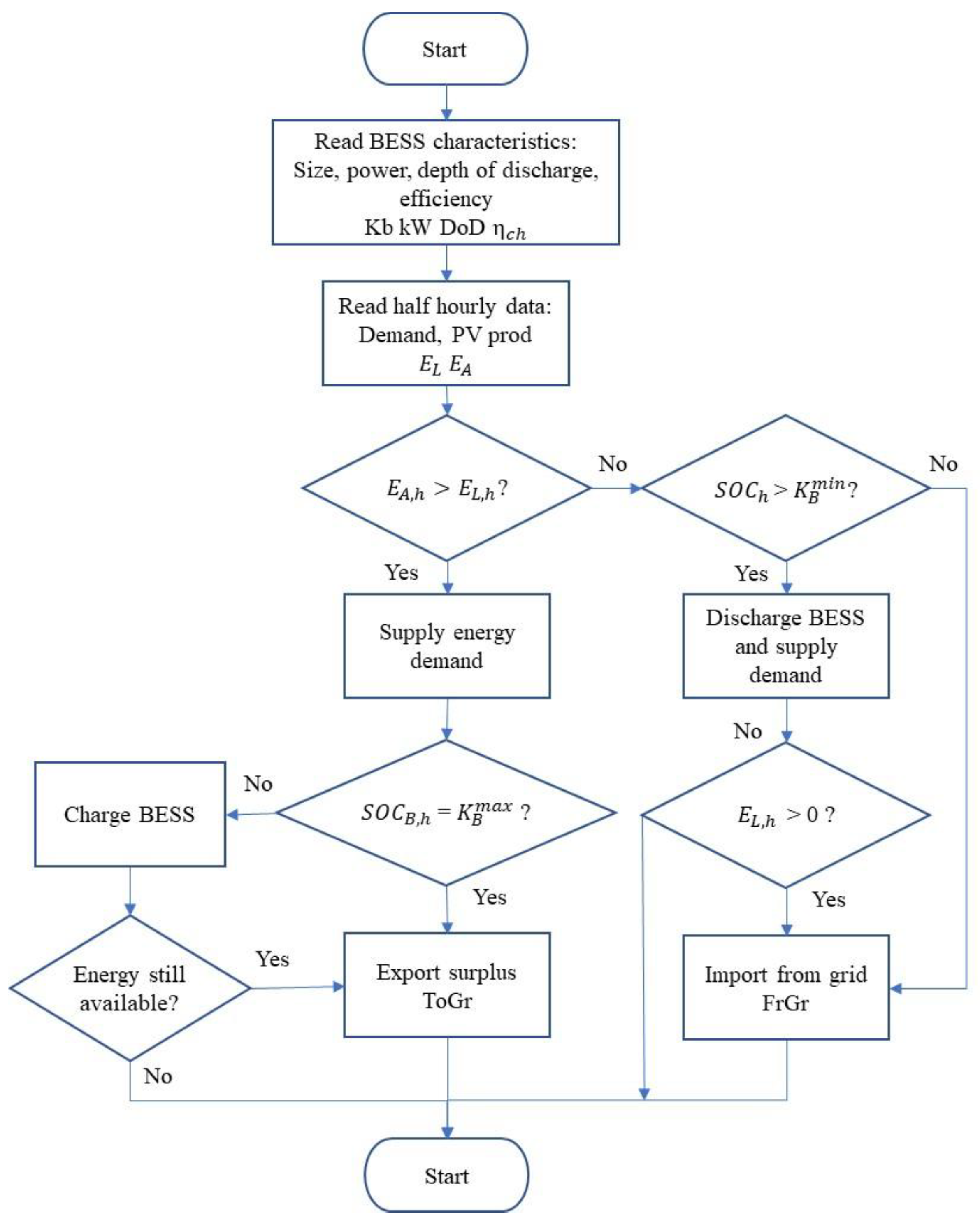
For the purposes of this paper, the BESS will be charged by PV and or grid imports during off-peak periods and dispatched during peak periods (as defined by residential tariffs), until exhaustion. A flowchart describing this process is presented in Figure 2.

2.4. Economic Model

The interaction of the household and network models will be evaluated across a range of economic measures. Through the resulting changes in area maximum, and volume, of demand the network economic impact can be evaluated through capital spending implications, changes in reliability measures, as well as the value of losses saved on the energy not served. This will be in addition to the measures commonly used in the literature reviewed of equipment lifecycle costs, energy displaced, and energy sales at FiT. Economic inputs to the economic model include:

Capex—A range of PV units will be applied across the test network to reflect those currently available and typically installed in the Australian market and is presented in

Table 3. PV system installed costs.

PV Input Parameters	PV1	PV2	PV3	Unit
Size	1.5	3	5	kW
Cost	2100	5000	7500	$AUD
Lifespan	25	25	25	year
Degradation/year	0.5	0.5	0.5	% [54]
Reference temp	25	25	25	C
Panel yield	15	15	15	%

Source: SolarQuotes 2017 [56].

.

The BESS product range under consideration is shown in

Table 4. BESS input parameters.

BESS Input Parameters	Sonnen Batterie Eco	Fronius Solar Battery	Tesla Powerwall	Units
Cost	8900	12,250	10,350	$AUD
Capacity	4	9	13.5	kWh
Cost per kWh	2225	1361	767	$/kWh
Capex reduction/year	5	5	5	%
Efficiency	86%	90%	90%	%
Power	2	4.8	7	kW
Degradation/year	3.5	3.5	3.5	%
Cycles	10,000/10 year	20 year	5000/10 year	-
DoD	100%	80%	100%	%

Source: Product specifications and fact sheets [55,56,58,59].

. The costs quoted are as installed including inverter. The model will assume replacement BESS are to the same specifications as originally. The model will be run across scenarios of projected price reduction forecasts. Based on cumulative manufactured capacity, stationary BESS units costs are forecast to fall to a range of $USD 290–520 by 2030, noting that the Tesla Powerwall option already falls within this range [57]. Due to the uncertainty of outlook regarding BESS cost curves a conservative 5% Year on Year (YoY) reduction will be applied to the base case BESS costs. Operational and maintenance spending is assumed to be $0 for household PV and BSS kit [57].

Retail and feed-in-tariffs—Residential retail peak and off-peak electricity prices from AGL NSW retail prices will be used to both provide the baseline i.e., no renewables scenario, and the value of energy imported from the grid during periods where demand is not met by PV, and when charging BESS as shown in

Table 5. Retail and price input parameters.

Cost Parameters	Value	Units
Peak	31.9	c/kWh
Off-peak—Controlled load	15.4	c/kWh
Daily charge	105.6	c/kWh
FiT	11.1	c/kWh
CPI	2.5	%
Demand growth	2	%
WACC	4	%
Distribution loss factor	1.0516	% [60]
Marginal loss factor	0.9926	% [61]

Source: AGL 2017 [62].

.

Grid prices—NSW wholesale prices simulated, as per Section 2.1.3 using AEMO historical data, for one year at half hourly level to value energy losses avoided.

The economic outputs will be expressed in terms of a range of project profitability measures to determine the value of investment impact; the measures utilized:

Net present value (NPV)—The financial evaluation of household economics will be based on a discounted cash flow analysis of the cash flows resulting from energy purchases and sales in addition to capital replacement cycles. In project profitability analysis, a positive NPV indicates that all costs are met, and the desired rate of return achieved. The weighted average cost of capital (WACC) is the measure used for that return. A WACC of 4% will be used for this modelling.

$$\mathrm{NPV}= {\displaystyle \sum }_{\mathrm{j}=1}^{\mathrm{n}}\frac{{\mathrm{RL}}_{\mathrm{j}}}{{\left(1+\mathrm{a}\right)}^{\mathrm{j}}}- {\displaystyle \sum }_{\mathrm{j}=0}^{\mathrm{n}-1}\frac{{\mathrm{I}}_{\mathrm{j}}}{{\left(1+\mathrm{a}\right)}^{\mathrm{j}}}$$

(12)

Internal rate of return (IRR)—The internal rate of return is used to calculate the profitability of a project. It is the rate of return such that would return an NPV of zero [63].

$${\displaystyle \sum }_{\mathrm{j}=1}^{\mathrm{n}}\frac{{\mathrm{RL}}_{\mathrm{j}}}{{\left(1+\mathrm{IRR}\right)}^{\mathrm{j}}}- {\displaystyle \sum }_{\mathrm{j}=0}^{\mathrm{n}-1}\frac{{\mathrm{I}}_{\mathrm{j}}}{{\left(1+\mathrm{IRR}\right)}^{\mathrm{j}}}=0$$

(13)

Levelized cost of energy (LCOE)—The net present value of per unit of electricity consumed in the household sector. This will provide a complementary measure of the resulting cost of electricity to the household against the retail tariff baseline [64]. Further, that as a proportion of demand will still be met from the grid that the LCOE used for this analysis will be a whole of system measure including capital costs, replacement capital, import costs, export sales and all associated tariffs represented as net costs ${\mathrm{C}}_{\mathrm{j}}$ in Equation (14).

$$\mathrm{LCOE}= \frac{{{\displaystyle \sum }}_{\mathrm{j}=1}^{\mathrm{n}}\frac{{\mathrm{C}}_{\mathrm{j}}}{{\left(1+\mathrm{a}\right)}^{\mathrm{j}}}}{{{\displaystyle \sum }}_{\mathrm{j}=1}^{\mathrm{n}}\frac{{\mathrm{E}}_{\mathrm{j}}}{{\left(1+\mathrm{a}\right)}^{\mathrm{j}}}}$$

(14)

Value of deferred augmentation (VDA)—The most common measures of network benefits have focused on network augmentation deferral and expressed the value per kVa or kW of capacity displaced [41,43,65,66]. For the purposes of this study, the figure of $810/kW/pa (escalated to 2017$) for the Ausgrid DSNP will be used [44]. With network planning determined by infrequently occurring maximum demand conditions, the use of DG for ‘peak shaving’ can result in a more efficient utilization of the network. For the purposes of this analysis VDA will be allocated to households based on the postage stamp (PS) method whereby benefits, or costs, are allocated to households based on their reductions to demand at the system peak demand period [7]. The benefit of the method being its simplicity and in focusing the analysis on the primary driver of network spending in system maximum demand.

Value of customer reliability (VCR)—Currently in the national electricity market (NEM), planning methodologies a VCR calculation is provided to network operators for use in prioritizing network capital planning [67]. The VCR represents in $/kWh the value placed on the reliable supply of electricity. Based on a review of market participants AEMO determined VCR values by region and industry type.

Table 6. NEM level VCR results $/kWh.

Customer Class	Residential	Agriculture	Commercial	Industrial	Direct Connect Customers	Aggregate NEM Value
VCR	25.95	47.67	44.72	44.06	6.05	33.46

Source: AEMO VCR Final Report 2014 p.2.

shows the NEM level VCR by customer type. The measure is used in the prioritization of network reliability spending where the amount is calculated by the customers demand × VCR × probability of outage of supply event. This amount is then used to determine the value of an outage and thus quantify the risk as an input to planning processes. VCR in this analysis will be used to measure a household’s value of reliability based on its average BESS State of Charge (SOC) as the measure of its self-sufficiency in the event of an outage.

Reduced losses—An important network benefit of DG is the reduction in losses resulting from generation being sited close to demand. Studies have shown that losses can be significantly reduced through the siting of DG units [11,68,69]. Such studies have found that DG can supply a portion of real and reactive power to the load thus reducing current and resulting losses. New South Wales grid prices will be applied to the energy loss avoided to value the benefit.

Through this analysis, it is possible to gain a clearer idea of the overall impact on the network of investment decisions taken at the household level. Where there is an asymmetry of benefits/costs the efficiency of network planning processes is impaired, and it is only through a clear alignment of incentives and investment decisions that energy networks can access greater efficiencies on offer through a more collaborative relationship with households.

3. Results and Discussion

Based on the methodologies detailed in the previous section 200 simulations were conducted at the half-hourly level for each household for one year using the QUT high performance computing (HPC) array. At each time step temperature, total sky cover, grid prices, global irradiation, and demand were simulated. A deterministic model of PV energy production was combined with a standardized household BESS charging regime.

3.1. Weather and Price Simulation Outputs Verification

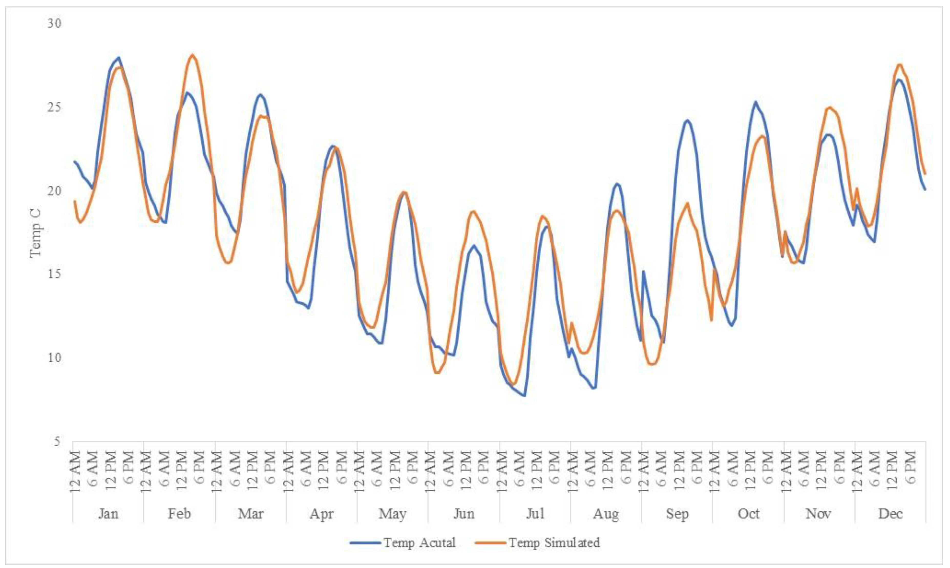
The resulting temperature simulation results based on the methodology outlined in Section 2.1.2 was compared to 12 months of historical data. As shown in Figure 3, the simulated data is shown to be an acceptable fit against the monthly half-hourly profile of historical data, while returning a mean absolute percentage error (MAPE) of 25.98.

Similarly, TSC simulations were plotted against historical data as shown in Figure 4.

The results for the simulation of grid prices is shown in Figure 5. It returns a MAPE of 6.71% again noting that the priority of this work is the short-term stochasticity present in price data.

3.2. Demand Simulation Outputs

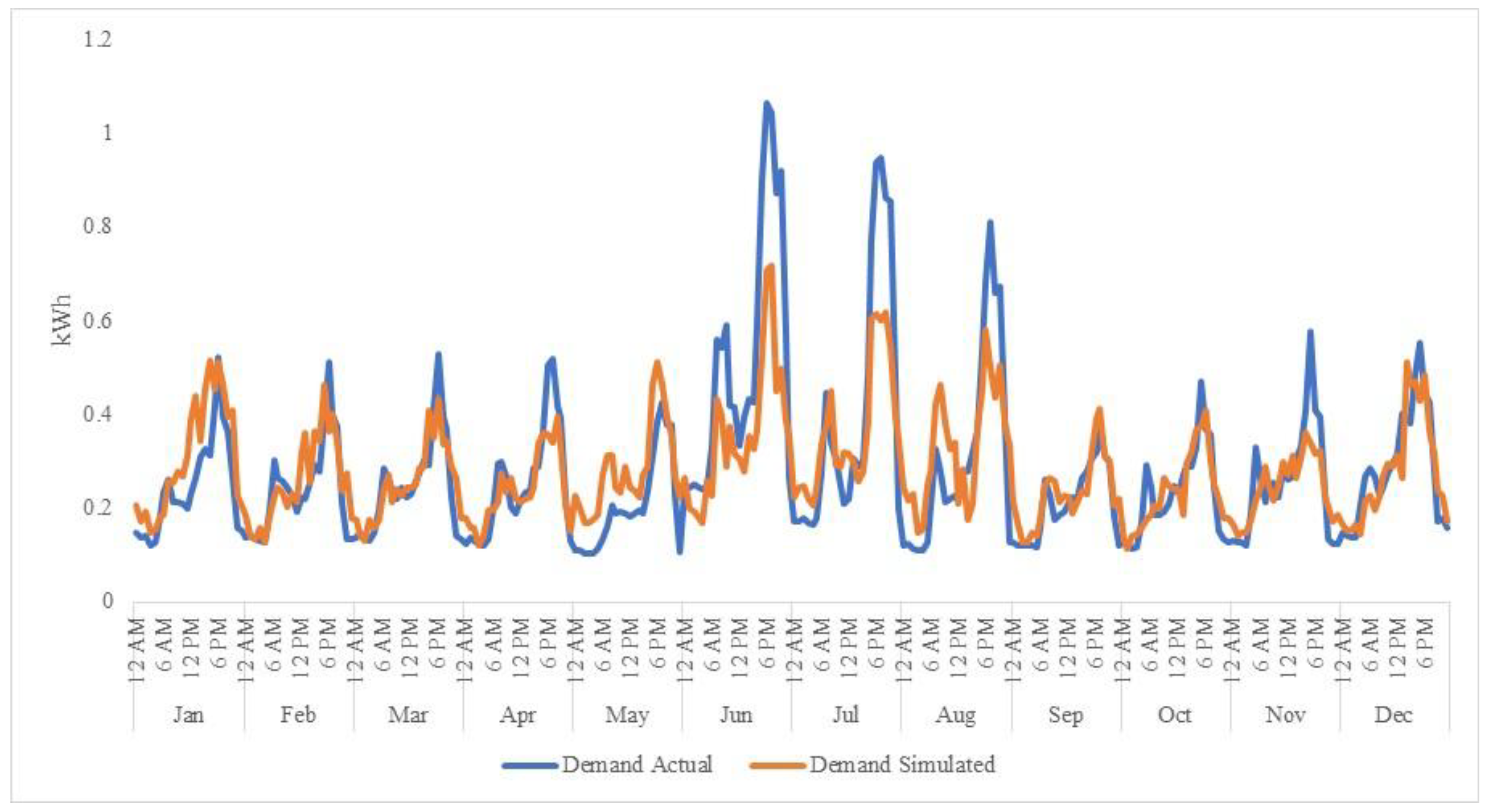
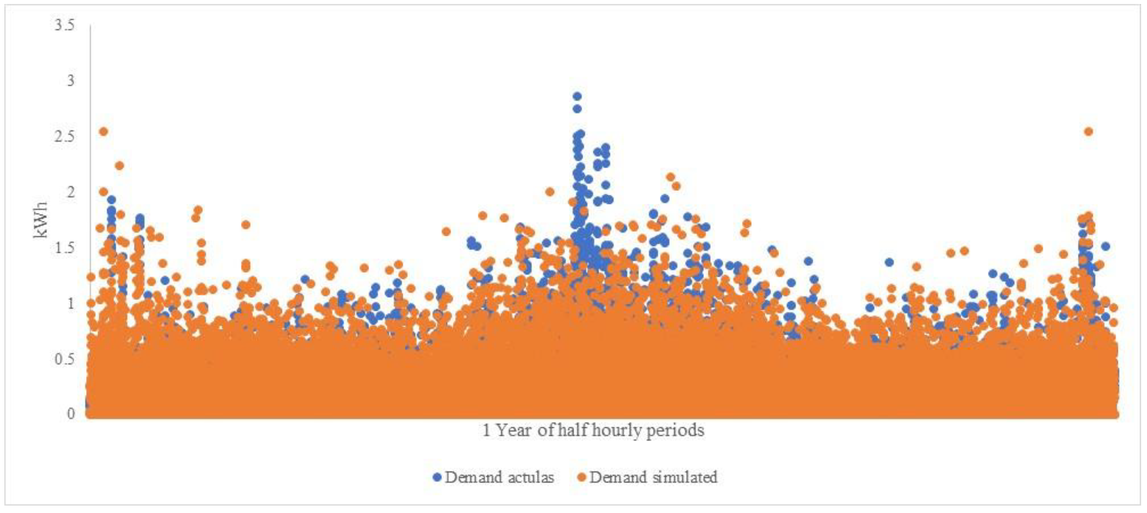
Household data from the SGSC project was analyzed to develop a simulation profile for use in multiple scenarios. The short-term stochasticity in household demand has led previous research to treat individual household demand as a random normally distributed variable [36,70]. However, due to the requirements of evaluating both the individual premise and the aggregated household sector, the characteristics of the aggregated housing sector are identified from a selection of 700 households covered in the SGSC data. The households selected were chosen due to completeness of demand data, location, and presence of household demographic data. Simulated household demand data was compared to a sample of historical data as shown in Figure 6 and reflects the increased in heating led demand in the winter months in NSW. Figure 7 compares forecasts and historical data at the half-hourly level for one year.

3.3. PV Production

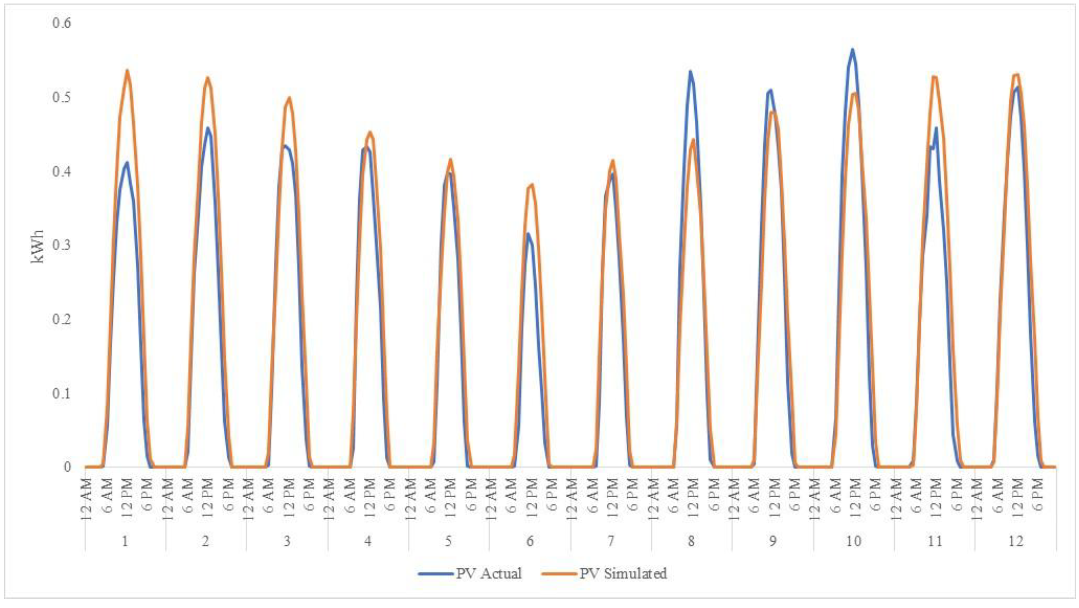
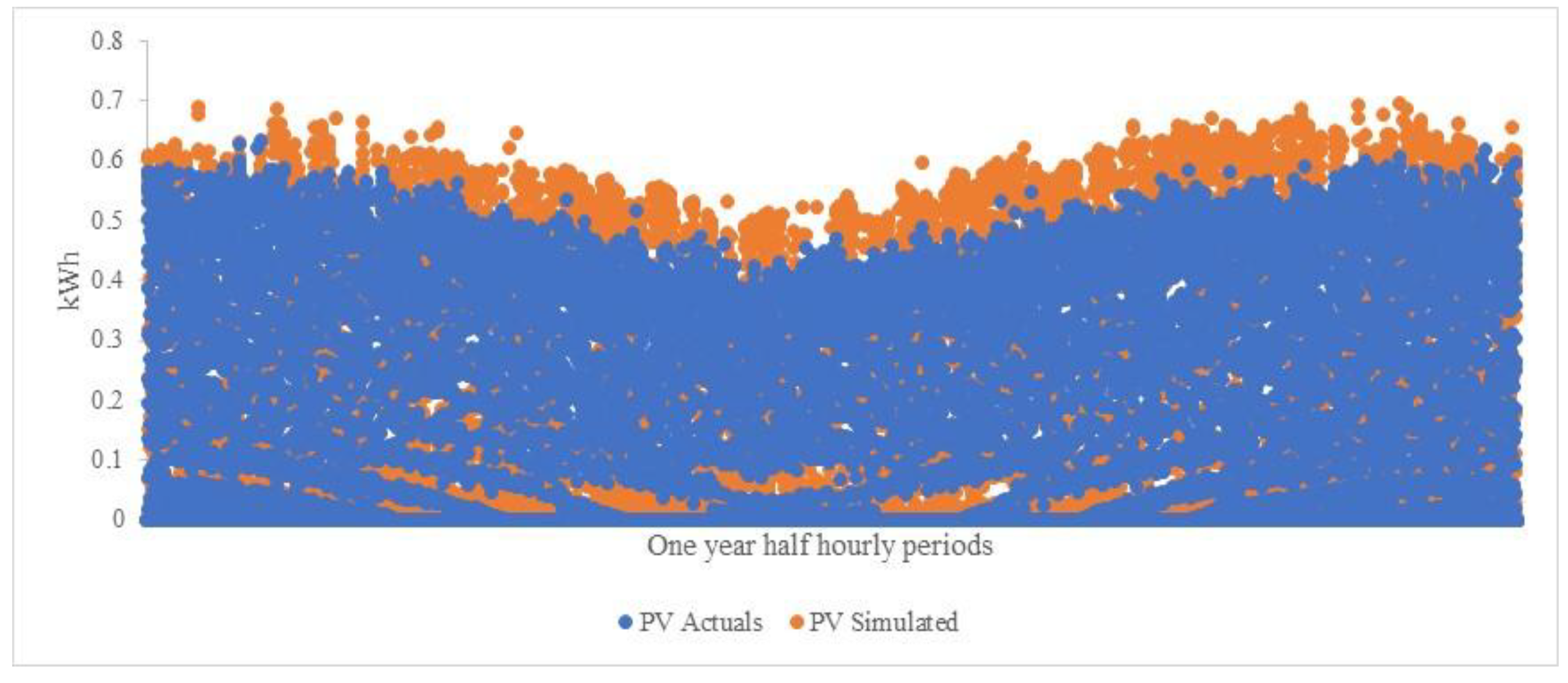
Based on the simulated cloud cover and temperature inputs half hourly PV energy production was calculated. These results were compared to data recorded in the Newcastle region in the SGSC trial. The resulting PV production simulation was compared against historical data for a 1.5 kW system in Figure 8 by half-hourly period and month, it shows that the scale and seasonality of annual PV production is reflected by the chosen simulation methods. Figure 9 presents a scatter plot of the results.

Based on the chosen simulation methods and their prediction performance as measured against historical data it was concluded that the combined model provides an effective basis for a detailed examination of a household’s energy production and consumption profile.

3.4. Operational Results

The model was run for 200 weather, price, and demand scenarios and the results analyzed. The baseline case involved peak and off-peak retail pricing and modelled the battery charging behavior to reflect an ‘off-peak only’ charging protocol of charging from surplus PV generation or during off-peak periods upon the exhaustion of the battery. The discussion of results is broken into household and area level analysis with operational and financial results presented respectively.

3.4.1. Household Operational Results

For comparison purposes a baseline demand was used, and each combination of equipment type evaluated,

Table 7. Household energy profile results by equipment mix, in kWh.

Equipment Mix	Baseline Energy	Peak Energy	Off-Peak Energy	PV	Exports	Imports	Peak Imports
1. PV 3 kW	6919	5028	1892	5112	2795	4602	2787
2. PV 5 kW	6919	5028	1892	8520	5772	4171	2390
3. PV 1.5 kW, BESS 4 kWh	6919	5028	1892	2556	431	4794	1501
4. PV 3 kW, BESS 4 kWh	6919	5028	1892	5112	2337	4144	926
5. PV 3 kW, BESS 9 kWh	6919	5028	1892	5112	2401	4209	164
6. PV 3 kW, BESS 13.5 kWh	6919	5028	1892	5112	2430	4238	14
7. PV 5 kW, BESS 4 kWh	6919	5028	1892	8520	5495	3894	744
8. PV 5 kW, BESS 9 kWh	6919	5028	1892	8520	5556	3955	101
9. PV 5 kW, BESS 13.5 kWh	6919	5028	1892	8520	5586	3985	4

Note: Peak periods as defined by retail contracts, 7 a.m.–10 p.m. weekdays.

presents the resulting changes in energy profiles in the first year of operation. As can be noted, there are dramatic reductions in the volume of peak energy imported across all BESS units, and with the 13.5 kWh BESS, combined with 3 kW PV and over, that effectively all peak period energy has been shifted to off-peak periods. The PV only results illustrate the issue of a timing mismatch between solar production and residential evening peak demands, a mismatch that BESS units effectively address.

In more detail,

Table 8. Peak energy shift analysis of 3 kW PV and 9 kWh BESS.

Peak Energy Shift—kWh	Baseline	PV and BESS
Baseline peak energy	5028	-
PV peak generation	-	5001
Imports peak	-	165
BESS supplied energy peak	-	2156
Exports peak	-	−2294
-	-	5028

Note: Retail peak periods are 7 a.m.–10 p.m. weekdays.

demonstrates the components of the peak shift and illustrates that at the reference demand level 3 kW of PV combined with 9 kWh BESS can effectively eliminate peak period imports.

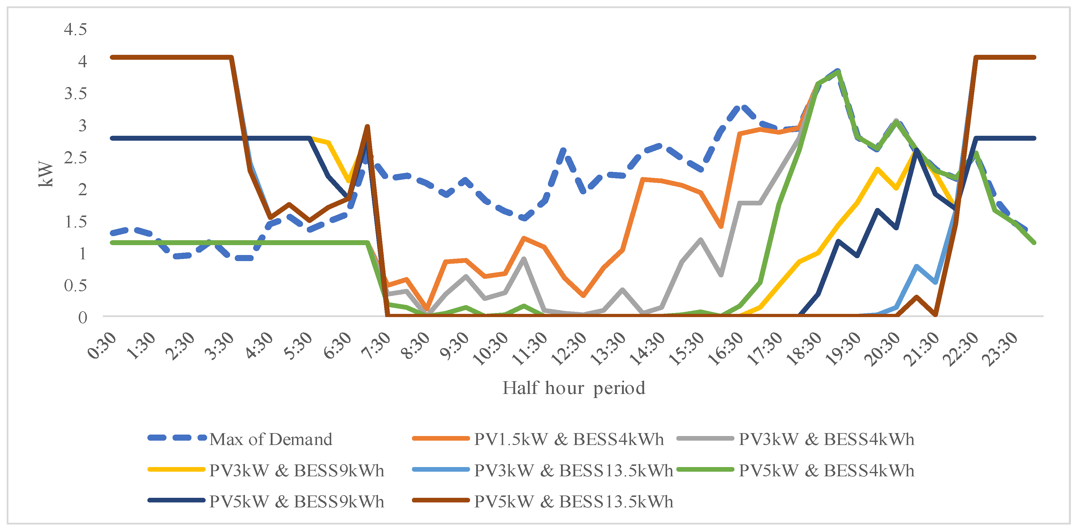
While reductions in peak period energy volumes can potentially result in more efficient use of the network it is the impacts on system maximum demand that can have the greater implications from a network planning perspective. The shift of demand out of the peak times can be seen in Figure 10 which compares household maximum demand, per 48 half-hour periods for the year, across equipment configurations against the baseline. Most notable is the shift in maximum demand to off-peak periods for the 13.5 kWh BESS units due to BESS charging, exceeding the previous baseline maximum. Further that the smaller capacity batteries exhaust circa period 29 (2:30 p.m.) and then commence charging. Where this is the case and ToU tariffs are available of peak (3 p.m.–9 p.m.), shoulder (7 a.m.–3 p.m. and 9 p.m.–10 p.m.) and off-peak(10 p.m.–7 a.m.) pricing further value could be gained by arbitraging the greater price differential between ToU peak and off-peak by dispatching only into the afternoon peak period.

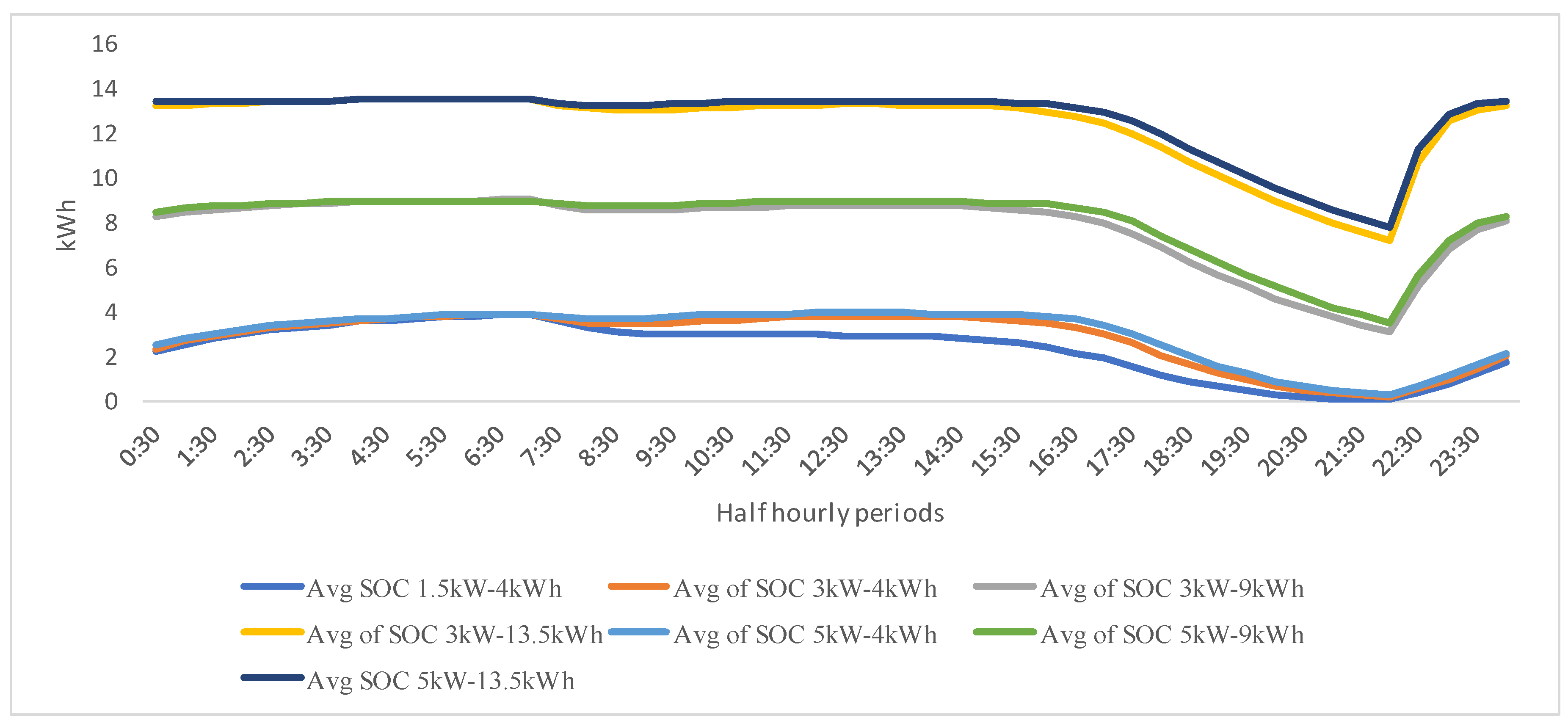
The BESS SOC profiles are displayed in Figure 11. It can be noted that the larger sized BESS units are not being used efficiently in the test demand scenario as on average they retain significant reserves at the completion of the peak period. That said, a household’s preference for longevity of the BESS through less cycling and preferred reserves in case of outage or intra-seasonal volatility would impact BESS utilization decisions. ToU optimization analysis is outside the scope of this paper.

3.4.2. Aggregate and Scenario Results

Simulations were run at 3, 10, 25, and 50% penetration rates of combined PV and BESS installations across the 166 subject households, kits allocated were configurations PV 1.5 kW and BSS 4 kWh, PV 3 kW and BSS 9 kWh, and PV 5 kW and BSS 13.5 kWh and the allocation was determined on household annual energy demand tertile.

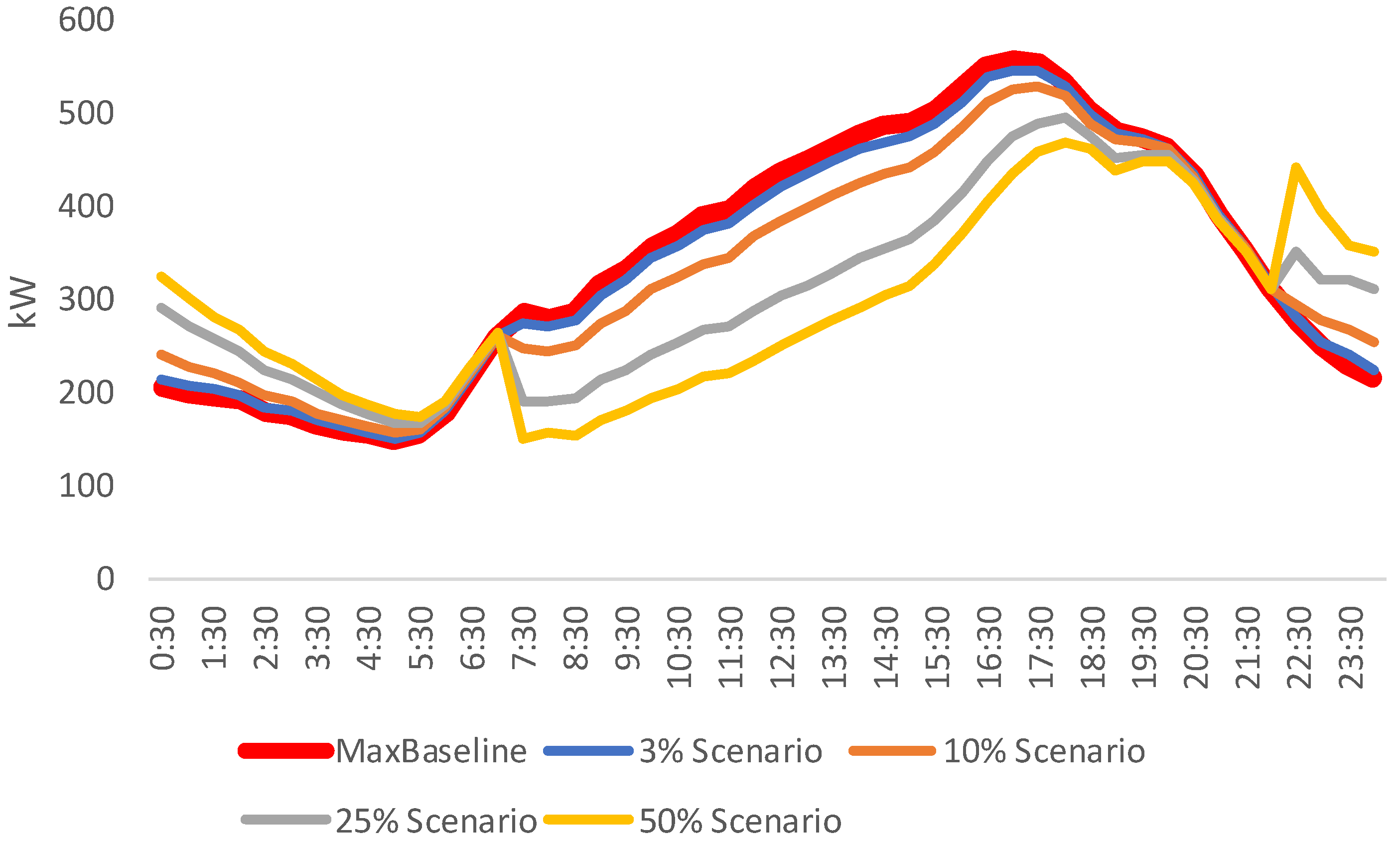
The scenario energy results are shown in

Table 9. Aggregate energy results by scenario.

Annual Aggregates	Baseline	3%	10%	25%	50%
Max demand, kW	558.6	548.4	529.7	495.1	470.6
Peak period energy, MWh	966.8	921.6	816.5	587.6	431.2
Off-peak period energy, MWh	338.2	352.1	384.6	452.7	498.6
Total energy served, MWh	1305.0	1273.7	1201.1	1040.4	929.9
Peak energy, %	74%	72%	68%	56%	46%

. The shift in energy consumption from peak to off-peak as noted in the individual household results is more pronounced at increasing levels of PV and BESS penetration. Achieving a reduction in maximum demand of 15.7% has significant capital planning implications in terms of potentially deferring network upgrades.

The impact of the maximum demand shift is most clearly demonstrated in Figure 12. The effects of higher rates of PV installation can be seen in the dramatic falls in demand from period 15:00 onwards compared to the baseline. The overall shape of residentially driven peak demand still holds, however, at 50% penetration it approaches the threshold for shifting the area maximum demand to off-peak (as defined under retail contracts) under these conditions.

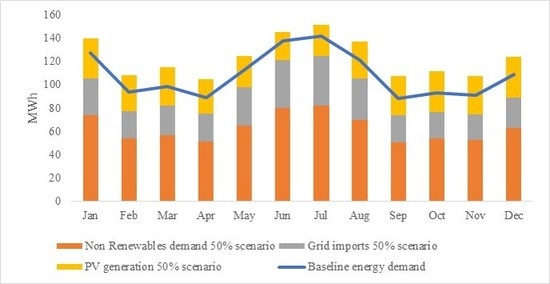
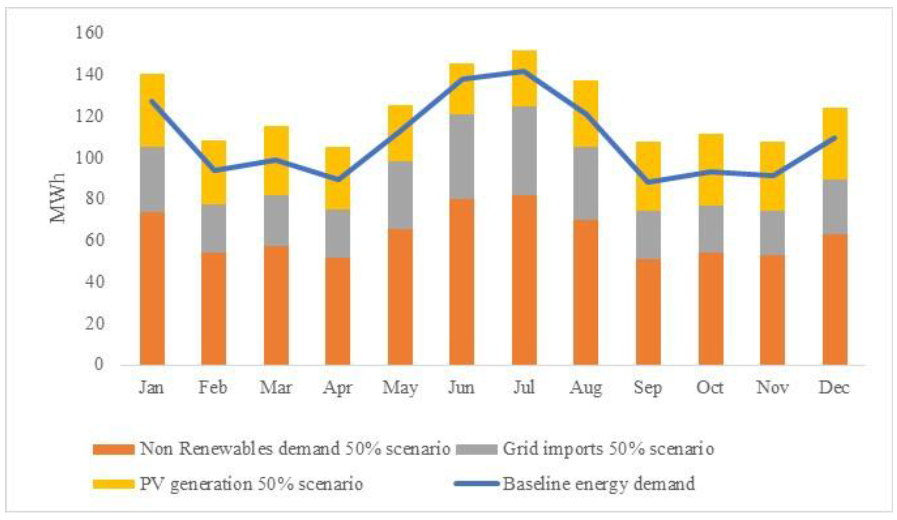
The changes to area energy supplied and its sources are indicated in Figure 13. In it the residual demand of the 50% of houses without PV and BESS is shown and the combination of imports and PV generation account for the difference against baseline with surplus PV generation exported.

3.5. Financial Results

A financial evaluation was conducted both at the individual household level and across scenarios with the results presented in economic outcomes both private and system wide which are attributable to household investment. The evaluation is conducted over the 25-year life cycle of PV panels with BESS replacement determined by manufacturer specifications regarding effective life and performance derating. The baseline for comparison is the present value of retail purchases with retail prices escalated at CPI of 2.5% and demand at load growth forecast of 2%.

3.5.1. Household Financial Results

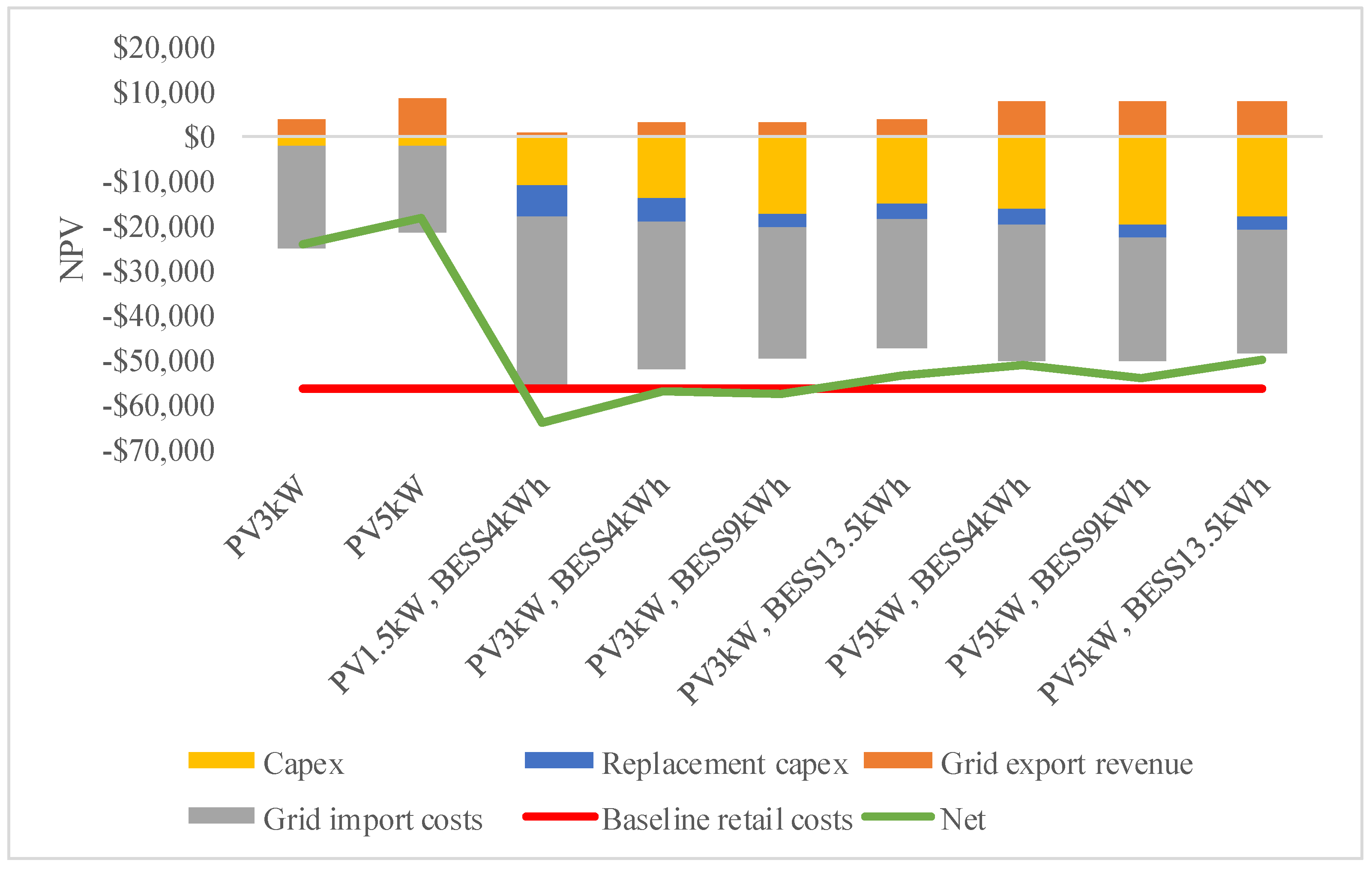
The household results are presented in

Table 10. Household financial results.

Equipment Mix	NPV Impact	NPV Impact%	VDA	Net	NPV Losses	NPV VCR	IRR	LCOE
1. PV 3 kW	$32,853	58%	$-	$32,853	$85	$-	59%	-$0.17
2. PV 5 kW	$38,345	68%	$-	$38,345	$101	$-	45%	-$0.13
3. PV 1.5 kW, BESS 4 kWh	-$7334	−13%	$8967	$1633	$84	$754	−0.2%	-$0.46
4. PV 3 kW, BESS 4 kWh	-$469	−1%	$11,260	$10,792	$109	$897	3.8%	-$0.41
5. PV 3 kW, BESS 9 kWh	-$1168	−2%	$13,050	$11,882	$108	$2462	3.6%	-$0.42
6.PV 3 kW, ESS 13.5 kWh	$2844	5%	$13,050	$15,894	$105	$3904	5.1%	-$0.39
7. PV 5 kW, BESS 4 kWh	$5473	10%	$11,644	$17,118	$119	$954	6.1%	-$0.37
8. PV 5 kW, BESS 9 kWh	$2626	5%	$13,050	$15,677	$116	$2537	4.9%	-$0.39
9.PV 5 kW, ESS 13.5 kWh	$6429	11%	$13,050	$19,479	$113	$3982	6.2%	-$0.36

. NPV evaluation shows that installing PV panels without BESS provides the greatest private economic returns. Considering combined systems, at current PV and BESS capex prices, results for households range from a significant private loss for the 1.5 kW PV combinations, and positive economic returns at higher levels of PV generation. However, on taking the network benefits into account, these private losses are offset by the contribution to reducing area maximum demand, as measured by VDA, and are further exceeded with improvements to value of reliability and losses avoided. Compared to a LCOE of the retail contract over the life of the analysis of -$.40/kWh that PV only options provide the lowest LCOE, combined kit options are close to grid parity and decline with the larger PV generation sizes.

In Figure 14, the components of the NPV results are detailed against the baseline of residential energy purchases. Energy imports still comprise the largest expense for all systems.

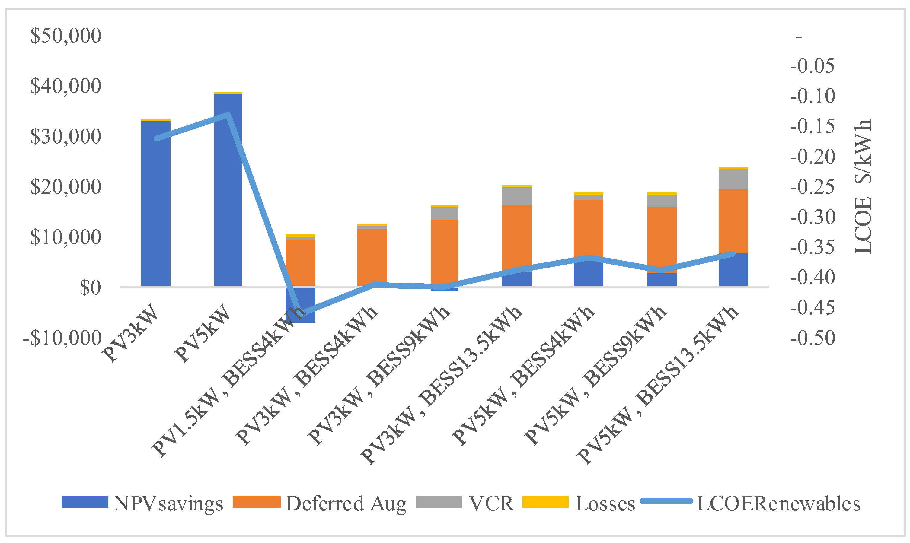
In Figure 15, the scale of the private and network benefits can be compared. With the current level of battery prices, the private investment case is marginal unless investing in the larger battery configurations. This raises social equity concerns as those households unable to afford the upfront investments will be unable to reduce their exposure to rising energy costs.

By considering the private investment in energy infrastructure by households and consequent system benefits, more efficient capital planning processes will include both sectors. With this more comprehensive view of economic impacts, the retrofitting of existing housing stock can play a greater role in a more rapid transformation and decarbonization of energy networks.

3.5.2. Sensitivities

Sensitivity analysis to retail price, demand and capex replacement costs were conducted across equipment mixes with the results displayed in

Table 11. Sensitivities to retail price, demand, and capex replacement, change in NPV savings %.

NPV Savings Impact	Retail Price			Demand			Cost of Rep Capex
Equipment Mix	+10%	+20%	+30%	+20%	+50%	+100%	−5%	−10%	−20%
1. PV 3 kW	0.3%	0.5%	0.7%	−7.0%	−15.0%	−24.4%	N/A	N/A	N/A
2. PV 5 kW	0.0%	0.0%	0.0%	−6.9%	−14.7%	−24.1%	N/A	N/A	N/A
3. PV 1.5 kW, BESS 4 kWh	4.0%	7.4%	10.2%	1.7%	−0.1%	−2.9%	7.0%	10.9%	14.8%
4. PV 3 kW, BESS 4 kWh	3.8%	7.0%	9.7%	2.5%	4.1%	0.3%	6.5%	9.6%	12.7%
5. PV 3 kW, BESS 9 kWh	4.5%	8.2%	11.3%	5.0%	9.1%	7.7%	4.8%	7.1%	9.8%
6. PV 3 kW, BESS 13.5 kWh	3.9%	7.2%	9.9%	5.3%	6.4%	5.9%	4.6%	6.9%	9.6%
7. PV 5 kW, BESS 4 kWh	3.2%	5.9%	8.1%	0.9%	3.3%	2.4%	4.2%	6.6%	9.2%
8. PV 5 kW, BESS 9 kWh	4.1%	7.5%	10.4%	5.6%	10.2%	11.1%	4.5%	6.6%	9.1%
9. PV 5 kW, BESS 13.5 kWh	3.5%	6.5%	8.9%	5.4%	7.8%	10.4%	4.3%	6.5%	8.9%

. Similarly, to Hoppman et al. [34], the sensitivity profitability of larger PV installs to increasing retail prices is pronounced. However, unlike Cuchhiella et al. [37] our results in PV only scenarios show that as demand increases profitability will suffer due to the increasing amount of peak demand unable to be displaced, so would view as unrealistic to have a 100% self-consumed PV scenario with household scale PV. A finding not dissimilar to that of Camillo et al. [71], that energy exported to the grid as opposed to displacing peak harms profitability. However, similarly our findings regarding PV and BESS private business case concur that they are uneconomic except at the larger configurations.

In our analysis for the least economic option, 1.5 kW PV and 4 kWh BESS, an increase of close to 20% in retail prices would be required to make the business case economical, whilst conversely increases to demand would have the opposite effect. An increase of the BESS price reduction factor to 15% YoY would be sufficient to render the same kit economic ceteris paribus. Note that the gains for the larger scale kits are marginal at increasing levels of demand once over 50%.

It is notable that, of the sensitivities considered here, the reduction in BESS costs is well under way and forecast to follow a path similar to that of PV. This trend which if exacerbated by the ‘death spiral’ effect on prices will result in an accelerating rate of transition of the network presenting a mounting challenge to network operators.

3.5.3. Aggregate and Scenario Results

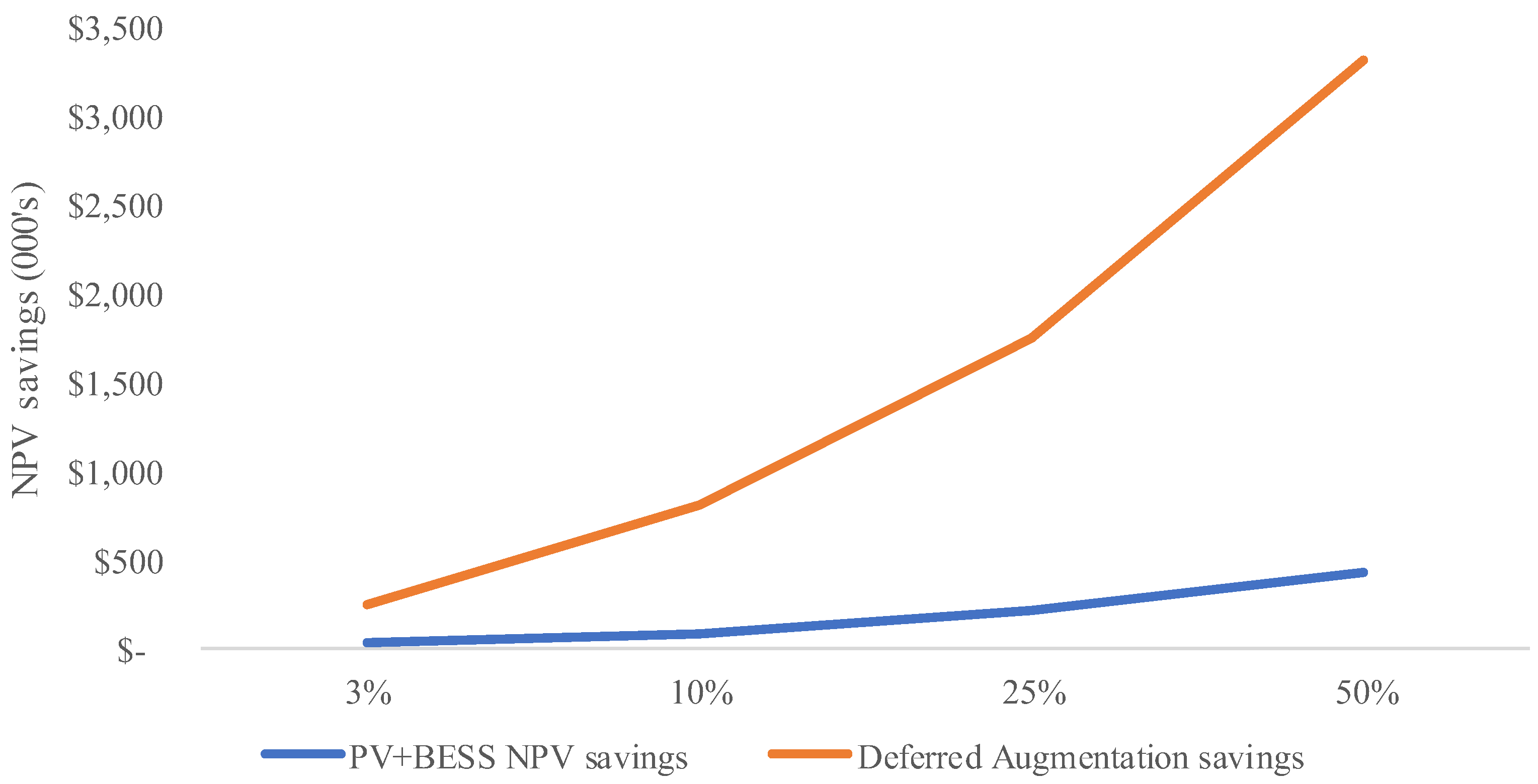
Analysis is conducted on the area level impacts to show the result of the household sector’s investment in energy infrastructure and ensuing network impacts. The aggregated sector results are shown in

Table 12. Twenty-five year financial results against baseline of retail power purchases.

Sector Aggregates	3%	10%	25%	50%
Household
Capex	$74,250	$246,000	$629,500	$1,270,000
PV + BESS NPV savings	$27,923	$65,665	$176,800	$351,710
PV + BESS NPV savings %	0.26%	0.62%	1.66%	3.30%
Network
Deferred Augmentation savings	$246,742	$802,257	$1,751,662	$3,318,151
VCR	$11,164	$36,106	$94,329	$188,967
Losses avoided	$592	$1858	$4743	$9606
Value of energy not served	$1618	$5367	$13,646	$19,325
% of Baseline wholesale energy cost	2.5%	8.2%	21.0%	29.7%

. For the purposes of this study, in the allocation of units to households no provision was made for profitability only demand level in determining the kit allocated. This has the effect of privately uneconomic installations being included. Their removal, whilst increasing the aggregated private benefit across scenarios would obscure the total potential area network benefits and so are included in the analysis. The network benefits arising from private household investment outweigh the private benefits to households at current prices.

From the results presented here, it can be stated that even under more conservative estimates of the value of deferred augmentation that investment in household PV and BESS can result in significant network savings. The reduction of maximum demand conditions being the primary driver of benefits, these results show that the promotion of a more rapid adoption of DG and storage is a viable option that can be funded through a prioritization of existing networks spending. This would result in a more efficiently utilized network and a reduction in distribution driven cost pressures on consumers.

The scale of the differential in private and network benefits is illustrated in Figure 16. This indicates that the network benefits from private investment in energy infrastructure must be considered in network capital planning. From an operational perspective, more collaborative relationships, such as the current demand management systems (DMS), could be utilized whereby DSNSPs purchasing reserve capacity of residential BESS to support the network in times of acute need. As the network transitions to a ‘thicker’ more resilient and data rich environment it will provide new tools for network operators to manage the network and respond to outages. However, this will require flexible and innovative schemes that incentivize prosumers to cooperate. This leads to a re-conceptualizing of energy networks to that of digitized platforms that are open to new entrants and innovative energy services, similar to the transition of the telecommunications industry. Following a similar path of transforming from a monopoly provided fixed radial network the digitization of telecommunications provided scope for the growth of mobile telephony and a competitive and flexible market with highly customizable solutions for consumers. Indeed, the digitized energy and telecommunications industries will be increasingly entwined through the fostering of smart technologies, whether it be household appliances, electric vehicles, smart metering, or network management [72].

4. Conclusions

This paper presents a model for a broader economic examination of the benefit or cost of investment decisions taken by households in terms of their impact on the capital planning of LV networks. This study contributes to the literature in several ways. Firstly, it bridges the gap between the household and network operator perspective in evaluating the wider impact of household investment decisions. Second, by evaluating the effect on customer reliability and reduced losses in addition to deferred network augmentation it demonstrates that DG and storage presents a powerful tool for improving the efficiency of networks. Prosumers have shown that they will invest in energy infrastructure and it is both a challenge and an opportunity for network operators to develop new ways to manage and plan networks collaboratively. Third, it presents a method for evaluating the scope for incentives for the household adoption of DG and storage to be funded by displacing network spending.

The results of the modelling show that where the private investment case does not support the installation of PV and BESS that the system benefits can outweigh these private losses. This has significant implications for determining policy support levels for the adoption of residential batteries. Further, that the modelling results show that when penetration levels approach 50% households installing PV and BESS in an area it can redefine area maximum demand. Given the residential contribution to maximum demand in Australia this indicates that residential batteries represent a significant opportunity to increase the efficiency of networks both in capital and utilization rates. To fully access the potential benefits on offer the transition to a network of prosumers will require new pricing structures and collaborative relationships between network operators and prosumers.

Specifically, this study aims to serve as analytical support to academics and policy makers in informing strategies for the contribution of retrofitting of existing housing stock with distributed generation and storage to the decarbonization of energy systems. With PV installed in over 17% of Australian households, how best to adapt existing control and pricing structures in response will have a significant impact on future adaptation strategies world-wide.

Further research will seek to integrate a detailed power flow model of the LV network to determine the impact of household investment decisions on network operations through the simulation of voltage and frequency maintenance requirements, thereby enhancing the analytical capabilities regarding network spending impacts as well as the increased capacity for the incorporation of higher levels of PV generation.

References

- CSIRO. Change and Choice: The Future Grid Forum’s Analysis of Australia’s Potential Electricity Pathways to 2050; CSIRO: Canberra, Australia, 2013.
- AER. State of the Energy Market 2017; AER: Melbourne, Australia, 2017. [Google Scholar]
- APVI. Mapping Australian Photovoltaic Installations; Australian PV Institute: Sydney, Australia, 2018. [Google Scholar]
- Queensland, Powerlink. Queensland’s Energy System Reliable as Electricity Demand Hits Record High. Available online: https://www.powerlink.com.au/About_Powerlink/News_and_Media/Media_releases/2017/Queensland_s_energy_system_reliable_as_electricity_demand_hits_record_high.aspx (accessed on 11 November 2017).
- AER. Final Decision: Ausgrid (Distribution) 2015–2019; Regulator, A.E., Ed.; AER: Melbourne, Australia, 2015. [Google Scholar]
- AER. Determinations & Access Arrangements. Available online: https://www.aer.gov.au/networks-pipelines/determinations-access-arrangements (accessed on 5 January 2018).
- Abdelmotteleb, I.; Roman, T.G.S.; Reneses, J. Distribution Network Cost Allocation Using a Locational and Temporal Cost Reflective Methodology. In Proceedings of the 2016 Power Systems Computation Conference (PSCC), Genova, Italy, 20–24 June 2016; pp. 1–7. [Google Scholar]
- Simshauser, P. From First Place to Last: The National Electricity Market’s Policy-Induced ‘Energy Market Death Spiral’. Aust. Econ. Rev. 2014, 47, 540–562. [Google Scholar] [CrossRef]
- Tonkoski, R.; Turcotte, D.; El-Fouly, T.H.M. Impact of High PV Penetration on Voltage Profiles in Residential Neighborhoods. IEEE Trans. Sustain. Energy 2012, 3, 518–527. [Google Scholar] [CrossRef]
- Thomson, M.; Infield, D.G. Network Power-Flow Analysis for a High Penetration of Distributed Generation. IEEE Trans. Power Syst. 2007, 22, 1157–1162. [Google Scholar] [CrossRef] [Green Version]
- Chiandone, M.; Campaner, R.; Pavan, A.M.; Sulligoi, G.; Mania, P.; Piccoli, G. Impact of Distributed Generation on power losses on an actual distribution network. In Proceedings of the 2014 International Conference on Renewable Energy Research and Application (ICRERA), Milwaukee, WI, USA, 19–22 October 2014; pp. 1007–1011. [Google Scholar]
- Diouf, B.; Pode, R. Potential of lithium-ion batteries in renewable energy. Renew. Energy 2015, 76, 375–380. [Google Scholar] [CrossRef]
- Darcovich, K.; Henquin, E.R.; Kenney, B.; Davidson, I.J.; Saldanha, N.; Beausoleil-Morrison, I. Higher-capacity lithium ion battery chemistries for improved residential energy storage with micro-cogeneration. Appl. Energy 2013, 111, 853. [Google Scholar] [CrossRef]
- Medina, P.; Bizuayehu, A.W.; Catalao, J.P.S.; Rodrigues, E.M.G.; Contreras, J. Electrical Energy Storage Systems: Technologies’ State-of-the-Art, Techno-economic Benefits and Applications Analysis. In Proceedings of the 2014 47th Hawaii International Conference on System Sciences (HICSS), Waikoloa, HI, USA, 6–9 January 2014; pp. 2295–2304. [Google Scholar]
- Divya, K.C.; Østergaard, J. Battery energy storage technology for power systems—An overview. Electr. Power Syst. Res. 2009, 79, 511–520. [Google Scholar] [CrossRef]
- Tant, J.; Geth, F.; Six, D.; Tant, P.; Driesen, J. Multiobjective Battery Storage to Improve PV Integration in Residential Distribution Grids. IEEE Trans. Sustain. Energy 2013, 4, 182–191. [Google Scholar] [CrossRef]
- Mohammad Taufiqul, A.; Amanullah, M.T.O.; Ali, A.B.M.S. Role of Energy Storage on Distribution Transformer Loading in Low Voltage Distribution Network. Smart Grid Renew. Energy 2013, 4, 236–251. [Google Scholar]
- Jayasekara, N.; Wolfs, P.; Masoum, M.A.S. An optimal management strategy for distributed storages in distribution networks with high penetrations of PV. Electr. Power Syst. Res. 2014, 116, 147–157. [Google Scholar] [CrossRef]
- Gast, N.; Tomozei, D.-C.; Le Boudec, J.-Y. Optimal Generation and Storage Scheduling in the Presence of Renewable Forecast Uncertainties. IEEE Trans. Smart Grid 2014, 5, 1328–1339. [Google Scholar] [CrossRef] [Green Version]
- Dunn, B.; Kamath, H.; Tarascon, J.-M. Electrical energy storage for the grid: A battery of choices. Science 2011, 334, 928–935. [Google Scholar] [CrossRef] [PubMed]
- Hashemi, S.; Ostergaard, J.; Yang, G. A Scenario-Based Approach for Energy Storage Capacity Determination in LV Grids with High PV Penetration. IEEE Trans. Smart Grid 2014, 5, 1514–1522. [Google Scholar] [CrossRef]
- Hoff, T.E.; Perez, R.; Margolis, R.M. Maximizing the value of customer-sited PV systems using storage and controls. Sol. Energy 2007, 81, 940–945. [Google Scholar] [CrossRef]
- Farhangi, H. The path of the smart grid. IEEE Power Energy Mag. 2010, 8, 18–28. [Google Scholar] [CrossRef]
- CER. Solar PV Systems with Concurrent Battery Storage Capacity by Year and State/Territory; Clean Energy Regulator: Canberra, Australia, 2018.
- Bhatti, M. From Consumers to Prosumers: Housing for a Sustainable Future. Hous. Stud. 1993, 8, 98–108. [Google Scholar] [CrossRef]
- Ritzer, G.; Dean, P.; Jurgenson, N. The Coming of Age of the Prosumer. Am. Behav. Sci. 2012, 56, 379–398. [Google Scholar] [CrossRef]
- Montoya, M.; Sherick, R.; Haralson, P.; Neal, R.; Yinger, R. Islands in the Storm: Integrating Microgrids into the Larger Grid. IEEE Power Energy Mag. 2013, 11, 33–39. [Google Scholar] [CrossRef]
- Dietrich, K.; Latorre, J.M.; Olmos, L.; Ramos, A. Modelling and assessing the impacts of self supply and market-revenue driven Virtual Power Plants. Electr. Power Syst. Res. 2015, 119, 462–470. [Google Scholar] [CrossRef]
- Mutale, J.; Strbac, G.; Pudjianto, D. Methodology for Cost Reflective Pricing of Distribution Networks with Distributed Generation. In Proceedings of the IEEE Power Engineering Society General Meeting, Tampa, FL, USA, 24–28 June 2007; pp. 1–5. [Google Scholar]
- Abeygunawardana, A.M.A.K.; Arefi, A.; Ledwich, G. Estimating and modeling of distribution network costs for designing cost-reflective network pricing schemes. In Proceedings of the 2015 IEEE Power & Energy Society General Meeting, Denver, CO, USA, 26–30 July 2015; pp. 1–5. [Google Scholar]
- Allan, G.; Eromenko, I.; Gilmartin, M.; Kockar, I.; McGregor, P. The economics of distributed energy generation: A literature review. Renew. Sustain. Energy Rev. 2015, 42, 543–556. [Google Scholar] [CrossRef]
- Santos, J.M.; Moura, P.S.; De Almeida, A.T. Technical and economic impact of residential electricity storage at local and grid level for Portugal. Appl. Energy 2014, 128, 254–264. [Google Scholar] [CrossRef]
- Masebinu, S.O.; Akinlabi, E.T.; Muzenda, E.; Aboyade, A.O. Techno-economics and environmental analysis of energy storage for a student residence under a South African time-of-use tariff rate. Energy 2017, 135, 413–429. [Google Scholar] [CrossRef]
- Hoppmann, J.; Volland, J.; Schmidt, T.S.; Hoffmann, V.H. The economic viability of battery storage for residential solar photovoltaic systems—A review and a simulation model. Renew. Sustain. Energy Rev. 2014, 39, 1101–1118. [Google Scholar] [CrossRef]
- Bortolini, M.; Gamberi, M.; Graziani, A. Technical and economic design of photovoltaic and battery energy storage system. Energy Convers. Manag. 2014, 86, 81–92. [Google Scholar] [CrossRef]
- Byrne, C.; Verbic, G. Feasibility of Residential Battery Storage for Energy Arbitrage; Australasian Committee for Power Engineering (ACPE): Perth, Australia, 2013; pp. 1–7. [Google Scholar]
- Cucchiella, F.; D’Adamo, I.; Gastaldi, M. Photovoltaic energy systems with battery storage for residential areas: An economic analysis. J. Clean. Prod. 2016, 131, 460–474. [Google Scholar] [CrossRef]
- Berrada, A.; Loudiyi, K.; Zorkani, I. Profitability, risk, and financial modeling of energy storage in residential and large scale applications. Energy 2017, 119, 94–109. [Google Scholar] [CrossRef]
- Changsong, C.; Shanxu, D.; Tao, C.; Bangyin, L.; Guozhen, H. Optimal Allocation and Economic Analysis of Energy Storage System in Microgrids. IEEE Trans. Power Electron. 2011, 26, 2762–2773. [Google Scholar]
- Farzan, F.; Lahiri, S.; Kleinberg, M.; Gharieh, K.; Farzan, F.; Jafari, M. Microgrids for Fun and Profit: The Economics of Installation Investments and Operations. IEEE Power Energy Mag. 2013, 11, 52–58. [Google Scholar] [CrossRef]
- Piccolo, A.; Siano, P. Evaluating the Impact of Network Investment Deferral on Distributed Generation Expansion. IEEE Trans. Power Syst. 2009, 23, 1559–1567. [Google Scholar] [CrossRef]
- Huang, S.; Xiao, J.; Pekny, J.F.; Reklaitis, G.V.; Liu, A.L. Quantifying System-Level Benefits from Distributed Solar and Energy Storage. J. Energy Eng. 2012, 138, 33–42. [Google Scholar]
- Gil, H.A.; Joos, G. Models for Quantifying the Economic Benefits of Distributed Generation. IEEE Trans. Power Syst. 2008, 23, 327–335. [Google Scholar] [CrossRef]
- AEMC. Power of Choice Review; Australian Energy Market Commission (AEMC): Sydney, Australia, 2012. [Google Scholar]
- Simpson, G. Network operators and the transition to decentralised electricity: An Australian socio-technical case study. Energy Policy 2017, 110, 422–433. [Google Scholar] [CrossRef]
- Copiello, S.; Gabrielli, L.; Bonifaci, P. Evaluation of energy retrofit in buildings under conditions of uncertainty: The prominence of the discount rate. Energy 2017, 137, 104–117. [Google Scholar] [CrossRef]
- Duenas, P.; Reneses, J.; Barquín, J. Dealing with multi-factor uncertainty in electricity markets by combining Monte Carlo simulation with spatial interpolation techniques. IET Gener. Transm. Distrib. 2011, 5, 323–331. [Google Scholar] [CrossRef]
- Modassar, C.; Jianzhong, W.; Nick, J. A sequential Monte Carlo model of the combined GB gas and electricity network. Energy Policy 2013, 62, 473. [Google Scholar]
- DIIS. Smart-Grid Smart-City Customer Trial Data. 2016. Available online: data.gov.au (accessed on 21 February 2017).
- Soares, L.J.; Medeiros, M.C. Modeling and forecasting short-term electricity load: A comparison of methods with an application to Brazilian data. Int. J. Forecast. 2008, 24, 630–644. [Google Scholar] [CrossRef]
- Box, G.E.P.; Jenkins, G.M.; Reinsel, G.C. Time Series Analysis: Forecasting and Control; J. Wiley & Sons: Hoboken, NJ, USA, 2008; Volume 4. [Google Scholar]
- Mathworks Inc. Curve Fitting Tool Box Users Guide (R2016b); Mathworks Inc.: Natick, MA, USA, 2016. [Google Scholar]
- Duffie, J.A.; Beckman, W.A. Solar Engineering of Thermal Processes; John Wiley & Sons: Hoboken, NJ, USA, 2013. [Google Scholar]
- Jordan, D.C.; Kurtz, S.R. Photovoltaic Degradation Rates—An Analytical Review. Progr. Photovolt. Res. Appl. 2013, 21, 12–29. [Google Scholar] [CrossRef]
- Tesla_Motors Tesla Motors Powerwall. Unit Prices and Performance Specifications Sourced. Available online: http://www.teslamotors.com/powerwall (accessed on 20 February 2018).
- SolarQuotes. Solar Panel Costs and Performances Specifications Sourced. Available online: https://www.solarquotes.com.au/panels/cost/ (accessed on 12 December 2017).
- Schmidt, O.; Hawkes, A.; Gambhir, A.; Staffell, I. The future cost of electrical energy storage based on experience rates. Nat. Energy 2017, 2, 17110. [Google Scholar] [CrossRef]
- Fronius. Battery Performance Specifications and Installed Costs Sourced. Available online: http://www.energymatters.com.au/wp-content/uploads/2016/03/fronius-energy-package.pdf (accessed on 20 February 2017).
- Enphase.AC. Battery Installed Costs and Performance Specifictations. Available online: https://enphase.com/en-au/support/enphase-ac-battery (accessed on 20 February 2017).
- AEMO. Distribution Loss Factors for the 2016/17 Financial Year; Operator, A.E.M., Ed.; Australian Energy Market Operator: Melbourne, Australia, 2016; Volume 3, p. 15. [Google Scholar]
- AEMO. Regions and Marginal Loss Factors: FY 2016–2017; Australian Energy Market Operator: Melbourne, Australia, 2016; p. 13. [Google Scholar]
- AGL Ltd. AGL Standard Retail Contracts. Retail Pricing for Peak and Offpeak Domestic Energy Use Sourced. Available online: https://www.agl.com.au/-/media/AGL/Residential/Documents/Regulatory/2017/2017-MY-PCP---AGL-NSW-Elec-website-pricing-final_070617.pdf?la=en (accessed on 12 February 2018).
- Talavera, D.L.; Nofuentes, G.; Aguilera, J. The internal rate of return of photovoltaic grid-connected systems: A comprehensive sensitivity analysis. Renew. Energy 2010, 35, 101–111. [Google Scholar] [CrossRef]
- Branker, K.; Pathak, M.J.M.; Pearce, J.M. A review of solar photovoltaic levelized cost of electricity. Renew. Sustain. Energy Rev. 2011, 15, 4470–4482. [Google Scholar] [CrossRef]
- Peterson, S.B.; Whitacre, J.F.; Apt, J. The economics of using plug-in hybrid electric vehicle battery packs for grid storage. J. Power Sources 2010, 195, 2377–2384. [Google Scholar] [CrossRef]
- Coles, L.R.; Chapel, S.W.; Iamucci, J.J. Valuation of modular generation, storage, and targeted demand-side management. IEEE Trans. Energy Convers. 1995, 10, 182–187. [Google Scholar] [CrossRef]
- AEMO. Value of Customer Reliability Review; Australian Energy Market Operator: Melbourne, Australia, 2014. [Google Scholar]
- Chiradeja, P. Benefit of Distributed Generation: A Line Loss Reduction Analysis. In Proceedings of the 2005 IEEE/PES Transmission and Distribution Conference and Exhibition: Asia and Pacific, Dalian, China, 18 August 2005; pp. 1–5. [Google Scholar]
- Marinopoulos, A.G.; Alexiadis, M.C.; Dokopoulos, P.S. Energy losses in a distribution line with distributed generation based on stochastic power flow. Electr. Power Syst. Res. 2011, 81, 1986–1994. [Google Scholar] [CrossRef]
- Conti, S.; Raiti, S. Probabilistic load flow using Monte Carlo techniques for distribution networks with photovoltaic generators. Sol. Energy 2007, 81, 1473–1481. [Google Scholar] [CrossRef]
- Camillo, F.M.; Castro, R.; Almeida, M.E.; Pires, V.F. Economic assessment of residential PV systems with self-consumption and storage in Portugal. Sol. Energy 2017, 150, 353–362. [Google Scholar] [CrossRef]
- Viola, R. Digitising the Energy Sector: An Opportunity for Europe. Managing Our Grids in Times of Increasing Shares of Renewables, Decentralised Generation and New Loads, Such as Electric Vehicles, but also for Creating New Value Streams (i.e., Services and Products). Smart Grids are Also Part of an Innovative and Competitive Energy Union. They Provide an Important Opportunity for European Manufacturers to Develop Attractive Smart Solutions and Boost Their Global Competitiveness. Available online: https://ec.europa.eu/digital-single-market/en/blog/digitising-energy-sector-opportunity-europe (accessed on 18 April 2018).
Figure 1.
Model architecture.
Figure 2.
Energy flow chart for each half-hourly period.
Figure 3.
Temperature simulation and historical data daily half hour averages by month.
Figure 4.
Simulated total sky cover and historical data daily half hour averages by month.
Figure 5.
Simulated and historical NSW grid prices daily half hour averages by month.
Figure 6.
Simulated household demand and historical data daily half hour averages by month.
Figure 7.
Simulated and historical household energy demand, 1 yr half-hourly.
Figure 8.
Simulated and historical PV generation, 1.5 kW PV system daily half hour averages by month.
Figure 9.
Simulated and historical PV production, 1 yr half-hourly.
Figure 10.
Maximum demand by equipment mix.
Figure 11.
BESS average SOC per period (kWh).
Figure 12.
Area maximum demand by scenario per half hour period.
Figure 13.
Net energy use, PV generation, and grid imports. 50% scenario.
Figure 14.
NPV value stack.
Figure 15.
Financial evaluation by equipment mix.
Figure 16.
Private and network savings by scenario.