State-of-Charge Estimation of Battery Pack under Varying Ambient Temperature Using an Adaptive Sequential Extreme Learning Machine


1
Faculty of Science, Agriculture and Engineering, Newcastle University Singapore, Singapore 599493, Singapore
2
School of Engineering, Temasek Polytechnic, 21 Tampines Avenue 1, Singapore 529757, Singapore
*
Author to whom correspondence should be addressed.
Energies 2018, 11(4), 711; https://doi.org/10.3390/en11040711
Submission received: 21 February 2018
/
Revised: 12 March 2018
/
Accepted: 13 March 2018
/
Published: 22 March 2018
(This article belongs to the Section D: Energy Storage and Application)
Abstract
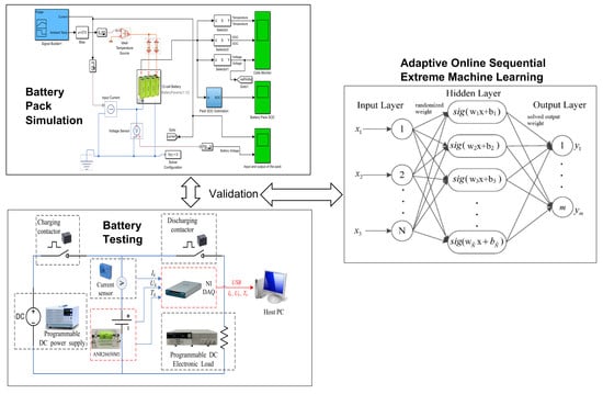
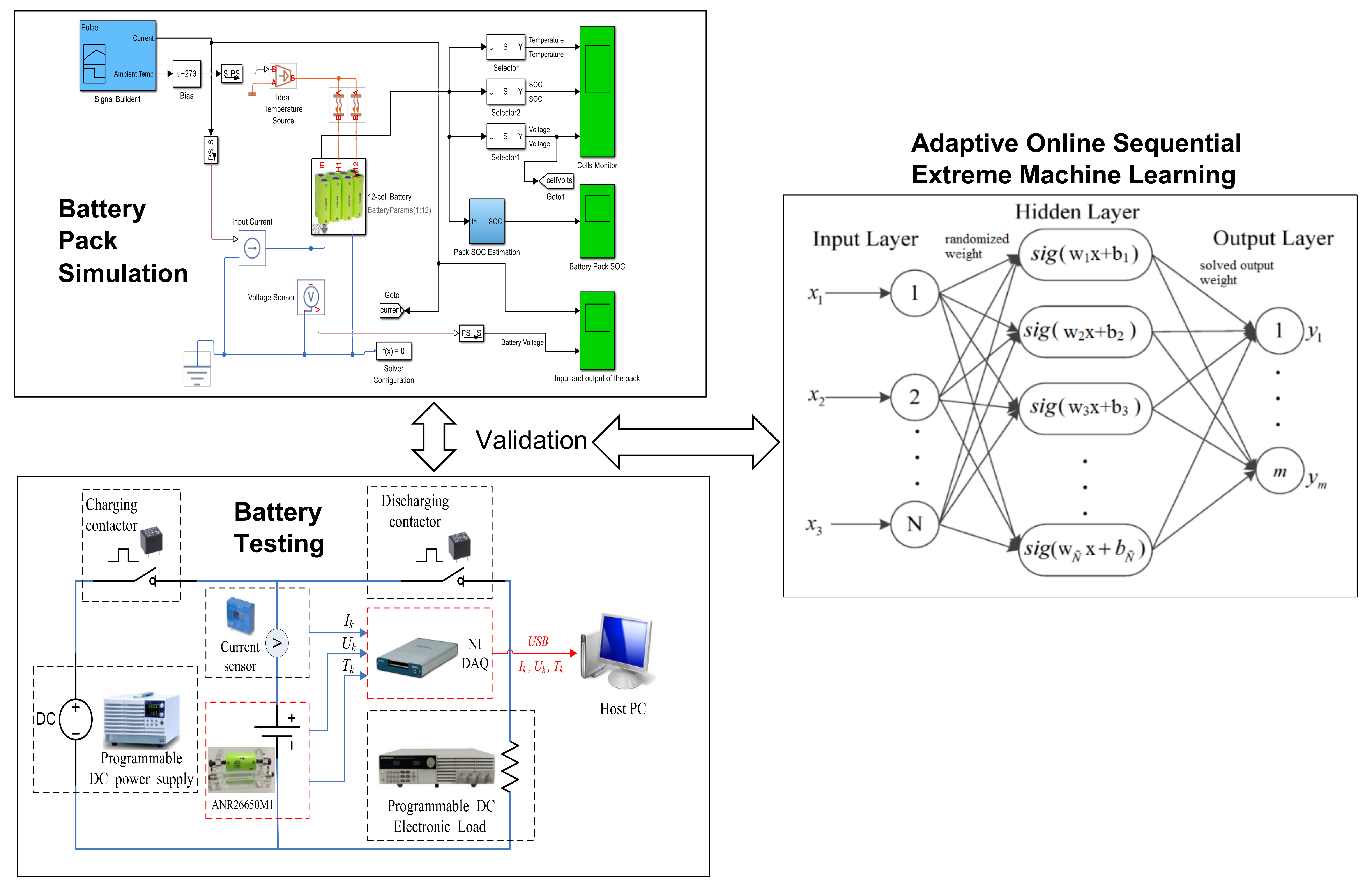
:An adaptive online sequential extreme learning machine (AOS-ELM) is proposed to predict the state-of-charge of the battery cells at different ambient temperatures. With limited samples and sequential data for training during the initial design stage, conventional neural network training gives higher errors and longer computing times when it maps the available inputs to SOC. The use of AOS-ELM allows a gradual increase in the dataset that can be time-consuming to obtain during the initial stage of the neural network training. The SOC prediction using AOS-ELM gives a smaller root mean squared error in testing (and small standard deviation in the trained results) and reasonable training time as compared to other types of ELM-based learnings and gradient-based machine learning. In addition, the subsequent identification of the cells’ static capacity and battery parameters from actual experiments is not required to estimate the SOC of each cell and the battery stack.
1. Introduction
Lithium iron phosphate (LiFePO4) batteries have become popular due to their high specific power, high specific energy density, long cycle life, low self-discharge rate and high discharge voltage for renewable energy storage devices, electric vehicles [1,2,3] and smart grids [4,5,6]. However, the batteries are vulnerable to the operating ambient temperature and unforeseen operating conditions such as being overly charged or discharged that could result in a reduced lifespan and deteriorate their performance. It is therefore vital to obtain the current state of charge (SOC) of the battery in actual application. The SOC is defined as the available capacity over its rated capacity in Ampere-hour (Ah). The estimation of SOC is quite complicated, as it depends on the type of cell, ambient temperature, internal temperature and the application. There have been many efforts in recent years to enhance the accuracy of the SOC estimation in battery management systems (BMSs) to improve the reliability, increase the lifetime and enhance the performance of batteries [7,8]. An accurate estimation of SOC could prevent sudden system failures resulting in damage to the battery power system. As a result, investigation on SOC estimation has spurred many research and development projects.
The common Ampere-hour method [8] uses the current reading of the battery over the operating period to calculate SOC values. However, the SOC need to be calibrated on a regular basis as its capacity could decline over the time. On the other hand, the voltage method uses the battery voltage and SOC relationship or discharge curve to determine the SOC. Both the Ampere-hour and voltage methods have disadvantages. The latter needs the battery to rest for a long duration and be cut off from the circuit to obtain the open circuit voltage, and the former suffers noise corruption and cumulative integration errors. In addition, the operating ambient temperature effects makes it quite difficult to estimate the correct SOC value. Another method using cell impedance for measuring both discharging and charging with an impedance analyzer was used, however, it is not commonly used in operating battery systems as it requires external instrumentation for measurement and validation.
Instead, a more accurate physical modeling using an electrochemical model was used [9,10,11,12]. The electrochemical models ensure the model parameters give have a proper physical meaning but the required nonlinear partial differential equations increase the complexity and computational efforts in the SOC estimation process. As a result, a model with fewer parameters in the electrochemical model was proposed [13] using moving horizon estimation to determine the SOC. For example, the equivalent circuit model [14,15,16] that depends on the value of the electronic components such as the resistors and capacitors was used. It was easier to obtain as compared to solving partial differential equations. However, the resistance and capacitance rely on the operating ambient temperature and the type of cell used in the battery. A few nonlinear observer design methods were applied to derive the ECM-based nonlinear SOC estimators such as sliding mode observer [17], adaptive model reference observer [18] and Lyapunov-based observer [19]. Despite its simplicity and less computational effort, it cannot represent the actual physical meaning of model parameters like the ambient temperature was not included in the model for the SOC estimation.
The equivalent circuit model using a Kalman filter (KF) [20,21,22,23] was another method employed to estimate the SOC. However, it requires a model of the battery and higher computing resources with correct initialization of parameters. The Extended KF (EKF) [20] was applied to estimate the SOC using a nonlinear ordinary differential equation model. The unscented KF was then used [21] to avoid the linearization of the nonlinear equation in the EKF. In addition, a nonlinear SOC estimator [22] are employed on the partial differential equations of the battery model.
The filtering performance could be enhanced using an online time-varying fading gain matrix. As a result, a strong tracking extended Kalman filter (STCKF) [23,24,25] that outperforms the EKF was used to track the state of sudden change of SOC value accurately. Cubature Kalman filter (CKF) [25] was utilized for a higher dimensional state estimation followed by a spherical cubature particle filter (SCPF) [26] for predicting the battery’s useful life. However, SCPF takes times to get the samples to congregate correctly, and it is difficult to determine the particle filter performance.
For the past few decades, artificial intelligence has been used to model complex systems with uncertainties. A data-driven approach using neural network [27,28,29], fuzzy logic [30], neural network-fuzzy [31], genetic algorithm-based fuzzy C-means (FCM) clustering techniques [32] to partition the training data and support vector machine (SVM) [33] were applied to predict the SOC. These machine learning methods require sufficient datasets and computation time for training and validating the SOC. The types of machine learning approaches used in the literature are numerous. In this study, the extreme learning machine (ELM) [34] will be used to model the state-of-charge of the battery pack. ELM has become quite useful due to its good generalization, fast training time, and universal approximation capability. As compared to other machine learning algorithms such as backpropagation (BP) [35], it is well-known that the parameters of hidden layers of the ELM are randomly generated without tuning. The hidden nodes could be determined from the training samples. Some researchers [23,36,37,38] have shown that the single layer feedforward networks (SLFNs) [39,40,41,42,43,44,45,46,47,48,49] ensure its universal approximation capability without changing the hidden layer parameters. ELM using regularized least squares could compute faster than the quadratic programming approach in gradient method adopted by BP. There is no issue of local minimal and instabilities caused by different learning rate, and differentiable activation function.
There are numerous types of ELM learning algorithms. The list in this paper is not exhaustive. A few selected algorithms will be briefly explained. Basic incremental ELM (I-ELM) [36,50] randomly produces the hidden nodes and analytically computes the output weights of SLFNs. I-ELM does not recompute the output weights of all the existing nodes when a new node is appended. The output weights of the existing nodes are then recalculated based on a convex optimization method when new hidden nodes are randomly added one at each time. The learning time for I-ELM is longer than ELM as it needs to compute n output weights one at a time when n hidden nodes are used. However, ELM only computes n output weights once when n hidden nodes are used. Few methods using different growth mechanism of hidden nodes were adopted. They are namely enhanced incremental ELM (EI-ELM) [51], error-minimized ELM (EM-ELM) [52] and optimal pruned ELM (OP-ELM) [53] that produce a more compact network and faster convergence speed than the basic I-ELM. Another incremental ELM, named bidirectional ELM (B-ELM) [54] with some hidden nodes not randomly selected could improve the error at initial learning stage at the expense of higher training time when compared to ELM. Another ELM learning using hierarchical ELM (H-ELM) [49] improves the learning performance of the original ELM due to its excellent training efficiency, but it increases the training time due to its deep feature learning.
On the other hand, the sequential learning algorithms are quite useful for feedforward networks with RBF nodes [48,55,56,57,58,59,60]. Some researchers [59,60] have simplified the sequential learning algorithms to enhance the training time, but it remains quite slow since data are handled one at a time instead of in batches. The online sequential extreme learning machine (OS-ELM) that can handle additive nodes (and RBF) in a unified framework from the batch learning ELM [36,61,62,63,64,65,66] is implemented in SLFNs. As compared to other sequential learning algorithms using different tuning parameters, OS-ELM requires the number of hidden nodes for tuning the networks solely. The newly arrived blocks or single observations (instead of the entire past data) are learned and removed after the learning process is accomplished. The input weights (connections between the input nodes to hidden nodes) and biases are randomly produced, and the output weights are analytically computed.
In the current literature, AOS-ELM applications to model the SOC of battery packs at different ambient temperatures has not been discussed. The application of AOS-ELM can converge quickly and sequentially with good generalization during the initial training stage where the data is progressively available in batches of small sample size from different cells. Moreover, the availability of the full data set for the design variables is often delayed by a lack of exact information during the early design stage that makes the sequential ELM based learning (that is crafted to handle newly arrived block or single observation) useful. In this paper, the SOC of the 12-cell will be estimated by Ampere-hour method to provide the output data set, and computation of the root mean square error (RMSE) of the AOS-ELM training and testing at different ambient temperature. As a result, the subsequent SOC estimation of the battery pack will be performed without extensive and time-consuming measurement using the Ampere-hour method (that needs frequent calibration of the cells’ static capacity and parameters from the actual experiments).
This paper has the following sections: Section 2 describes the SOC estimation process under different ambient temperature. Section 3 reviews on ELM and adaptive sequential ELM learnings on the SOC. Section 4 evaluates some commonly used EKF-based approach and other types of neural networks as compared to the ELM-based learning. Section 5 concludes the paper.
2. SOC Estimation
The equivalent circuit model (obtained in this section) using parameters such as resistors, voltage sources, current, capacitors and capacity in Ah are embedded into a series of online look-up tables at different ambient temperatures. By considering the SOC values at different ambient temperatures, it improves the robustness of the battery model due to cells’ aging. In addition, the SOC will be estimated by Ampere-hour method in order to provide the output data set for training and testing the neural networks and computation of the respective errors. The dataset will be used as the input and output parameters for subsequent neural network training. The SOC will be estimated from the neural network training. The information such as the static capacities, open-circuit voltage (OCV), resistors and capacitor can be obtained.
2.1. Battery Cell Equivalent Circuit Model
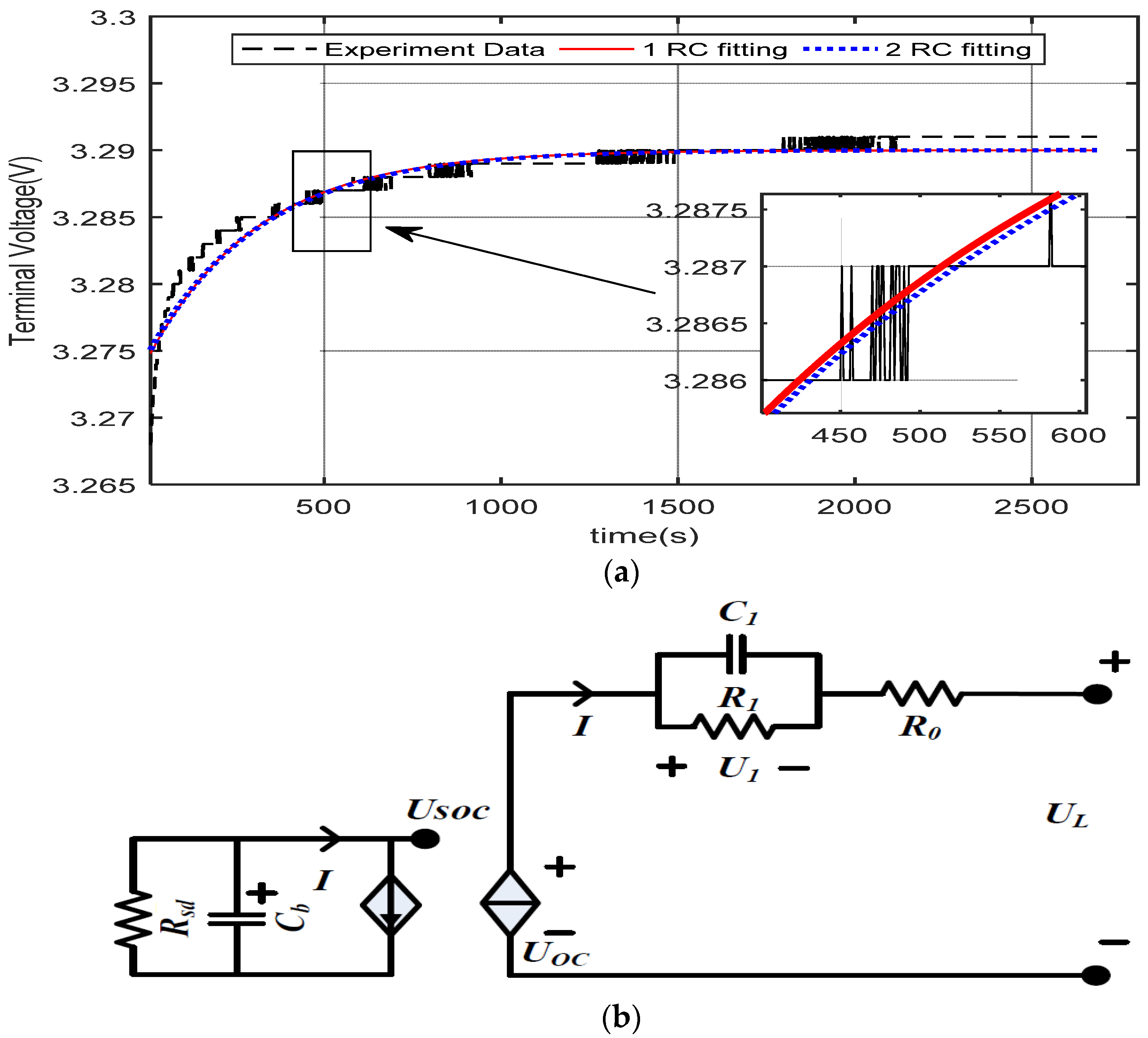
The number of RC blocks used in ECM can be different for various applications. As the number of RC blocks increases without significantly improves the accuracy of the terminal voltage (see Figure 1a), the single RC circuit is chosen as shown in Figure 1b.
The relationship between SOC to the open circuit voltage (OCV) is expressed by a voltage source defined as Uoc. R0 is the internal resistance. R1 and C1 simulates the transient response during discharge or charge process. The charge capacitor is denoted as Cb, in A·s, Rsd is the self-discharge energy loss as a result of long time storage. The voltages drop across C1 is U1. The current and terminal voltage are expressed as system output I and system input UL, respectively. The equation of the battery model can be defined as shown:
where I > 0 is charging and I < 0 is discharging. The critical parameters such as OCV, R0, R1 and C1 are used to estimate the SOC of the battery cells. To prevent the cells from undercharging or over-discharging, the SOC need to be computed accurately. In this paper, the SOC is determined as shown:
where Cn is the nominal capacity of the battery, SOC(0) is the initial SOC, T is the sampling time, i(t) is the load current, η is Coulombic efficiency, and Sd is the self-discharging rate. In this paper, the LiFePO4 cell is assumed as η = 1 (>0.994) under room temperature and Sd = 0.
The capacity of the battery pack in series configuration is determined by the electric charge stored in the cells expressed as the total minimum capacity:
where Ci is the capacity of the i-th cell, Cseries is the functional capacity of the battery pack, m is the total cells in series and SOCi is SOC of the i-th cell.
2.2. Parameters Identifications of Ambient Temperature-Dependent Battery Cell
The SOC will be sampled at step k, expressed as SOC(k). The SOC has a non-linear relationship with the battery cell voltage, current, capacity and ambient temperature. The voltage, current, and capacity were obtained from the test-bench under a few ambient temperatures such as 5, 15, 25 and 45 °C, as shown in Figure 2a. The reason for using the minimum temperature above 5 °C is due to the limitation of the temperature chamber at the time of the testing. The chamber could not reach freezing point. Hence, a temperature above 5 °C was used. The SOC(k) value of each cell was first estimated by the Ampere-hour method followed by the use of machine learning approach to predict the SOC. The Ampere-hour method was used as a reference to compute the RMSE of the training and testing.
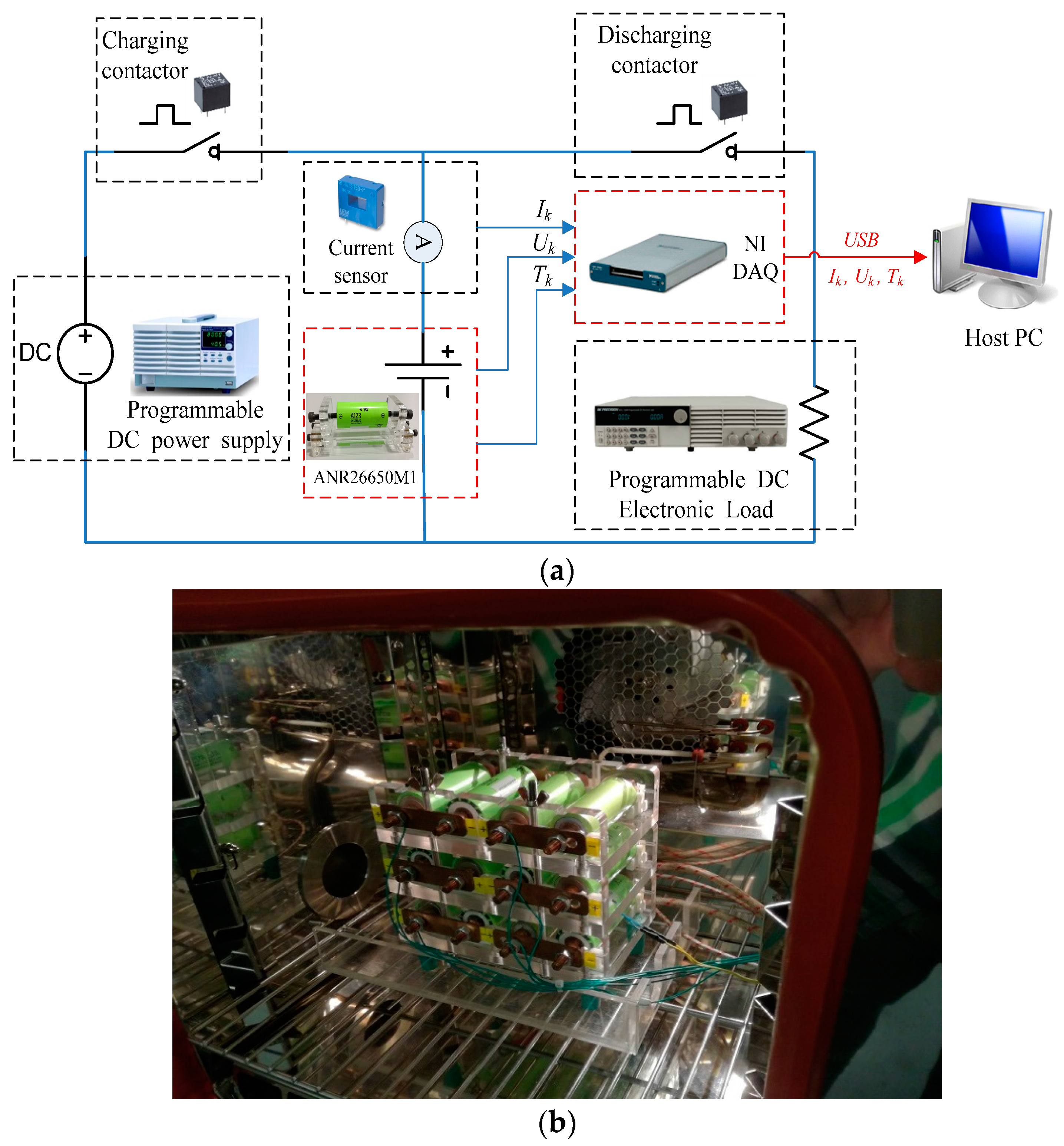
Twelve lithium iron phosphate battery cells (ANR26650M1-B) were used in the experiments. The specifications of the battery cells are tabulated in Table 1. The battery pack is positioned in an environmental chamber as illustrated in Figure 2b to investigate the battery power system performance under different ambient temperatures. The following ambient temperatures with an increment of 10 °C starting from 5 °C to 45 °C are pre-set into the chamber before the tests. The load current is generated by a DC electronic load while the battery cells are charged by a programmable DC power supply. It is used to control the voltage or current source with the output voltage (maximum at 36 V) and current (maximum at 20 A). The host PC communicates with the DAQ device to measure the charging and discharging of each cell. The NI DAQ device will control the outputs and inputs data with acquisition rate set to 1 sample per second. The temperature sensors are positioned within the battery’s enclosure to measure the ambient temperature around the cells. A current sensor will measure the current during the charging and discharge operation.
The host PC performs the 1-RC equivalent circuit modeling of the battery stack in MATLAB/Simulink environment using the data collected from the physical battery prototype. A few experiments were conducted to obtain the battery parameters such as Ah, OCV, R0, R1 and C1 of the battery. First, a Static Capacity Test [67] will be performed. The Ah of a battery cell ages and the value will differ from the nominal capacity. The static capacity testing will compute the Ah at a constant discharge current. The battery will be charged at 0.8 C rate (2 A) to the fully charged state in constant-current-constant-voltage (CCCV) mode under a specified temperature. The battery is fully charged to 3.6 V when the current reaches 1 mA. Then, apply a 45 min relaxation period before discharging the battery cell at a constant current 0.8 C rate until the voltage reaches the battery minimum limit of 2.5 V.
Second, a Cycling Aging Test [46] will be conducted. The cycling aging is important as the battery can lose its capacity over time. If the capacity decreases to approximately 80 percent of its nominal capacity, the battery is considered to reach its lifespan. The static capacity of the battery has a nonlinear relationship in the charge and discharge cycling as shown:
where Nc is the number of discharge and charge cycles.
Lastly, a Pulse Discharge Test [46] will be conducted. The battery voltage terminal response at different SOC and temperature are determined during the test. The test will generate a series of discharge pulses for the SOC range from 0 to 1 under different ambient temperatures. First, the battery is charged at 0.8 C rate (around 2 A) to the fully charged state in CCCV mode under a specified temperature. The battery is fully charged to 3.6 V when the current reaches 1 mA. Apply a 45 min relaxation period before discharging the battery cell at a pulse current 0.8 C rate with 450 s discharging time and 45 min relaxation period, until the terminal voltage reaches the cut-off voltage 2.5 V. As a result of the parameters identification of the 12-cell battery pack, and a few look-up tables for Ah, OCV, R0, R1 and C1 are tabulated in Table 2, Table 3 and Table 4, respectively. The Simscape model is used to simulate the battery cell. The results for each cell under different temperatures are shown in Table 2. As observed, the static capacities of the twelve battery cells are quite high at higher ambient temperature.
The open-circuit voltage (OCV) was determined from the Pulse Discharge Test. The OCV is the battery’s terminal voltage at equilibrium state obtained during the relaxation period. As seen in Figure 3, OCV vs. SOC curves at various temperatures is plotted. In Figure 3a, it is observed that there is a constant OCV for the SOC value from 0.1 to 0.9. As seen in Figure 3b, a different OCV at various temperatures can be observed. For SOC value of 0.2, the OCV is around 25 mV with an error of 10% in SOC. As a result, the OCV is unable to fit using a standard curve fitting approach. Instead, an adaptable look-up table of OCV values under different temperatures is used.
At different SOC and temperature conditions, the corresponding OCV of each battery cell will be stored in a 2-D look-up table as shown in Table 3. Figure 4 shows an example of an OCV look-up table for Cell #1. Similar OCV look-up table was established for Cell #2 to Cell #12 (they are not shown in this paper).
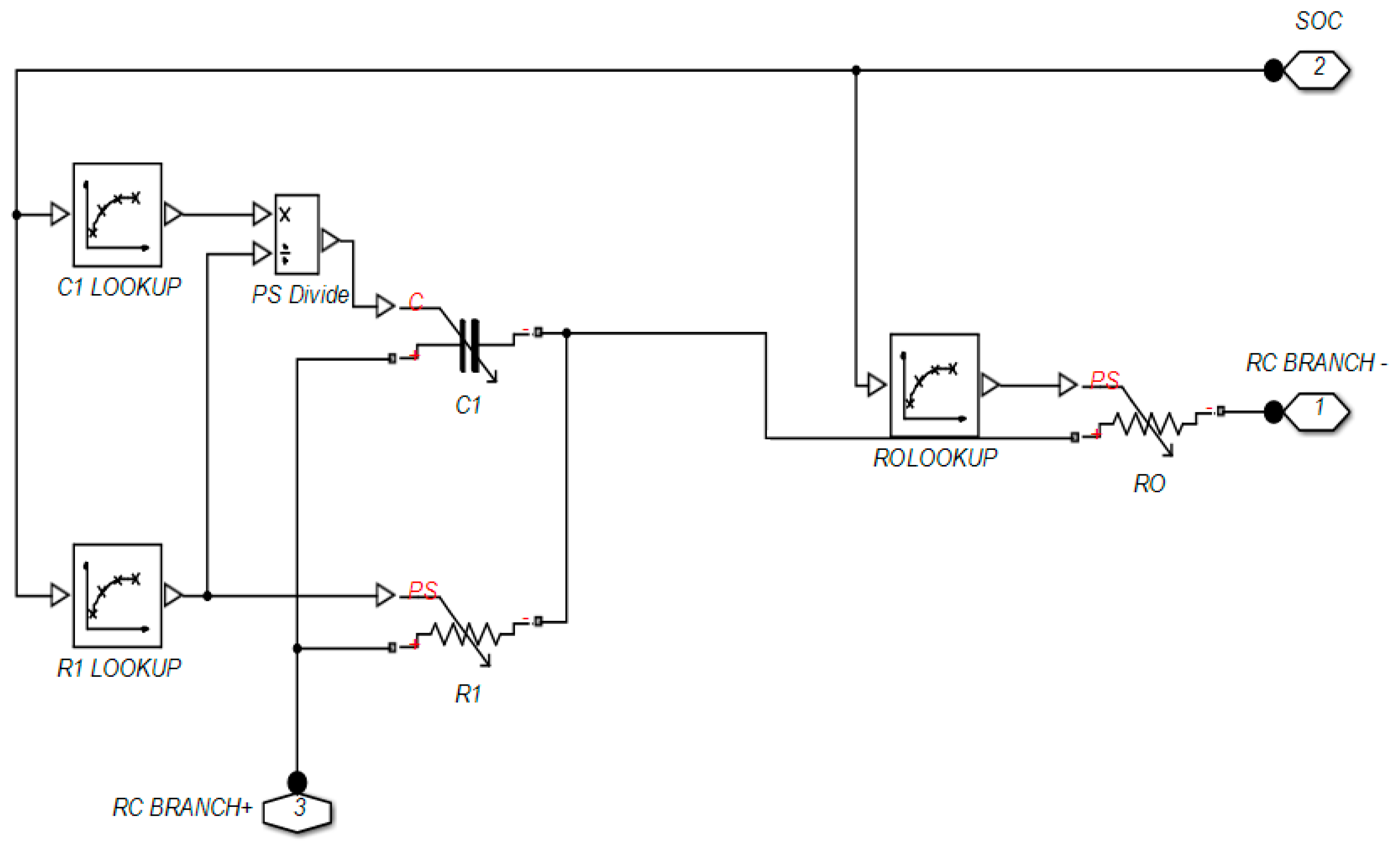
The cells’ parameters such as R0, R1 and C1 were estimated from the Pulse Discharge Test. The R0 was computed from the instantaneous increase of voltage in the terminal voltage over time curve. On the other hands, R1 and C1 were the transient response of the battery voltage during the relaxation period of the terminal voltage over the time curve. The parameters of the RC circuit were obtained in Table 4. These identified values together with static capacities and OCV at different SOC value were stored online in a series of 2D look-up table for subsequent machine learnings.
The proposed battery model using Simscape (see Figure 5) was validated by comparing the cell model at different temperatures with the experimental results obtained. As shown in Table 5, a per-unit (p.u.) was used to compare the root means square error (RMSE) between the simulated model and experimental results of the terminal voltage at various temperatures:
For example, 0.005-p.u. (equals to 0.5%) Implies the absolute RMSE of the terminal voltage was approximately 0.018 V based on the base terminal voltage of 3.57 V from the experiment (maximum expected value). As seen in Table 5, the RSME of the p.u (in percent) of terminal voltage was quite small across the cells at different ambient temperature. As observed in Figure 6, the experimental data at 35 °C (not used for the parameters identification) was compared with the simulation model to check the model robustness under a different temperature. The result shows that the battery model output can estimate the terminal voltage with small error as shown in Table 5. The RMSE of the terminal voltage can converge to zero. It shows the proposed ECM battery model in Figure 5 has some degree of robustness in estimating the terminal voltage.
2.3. SOC Estimation of Ambient Temperature-Dependent 12-Cell Battery Pack
The physical connection of the battery cells in series configuration can be seen in Figure 7a. Figure 7b shows the simulation model developed for the 12-cell battery instead of a single cell. The temperature sensors were physically placed at different locations at the top surface of the twelve cells to measure the changing ambient temperature in real-time. The microcontroller in the BMS will determine the corresponding battery model and the SOC values based on the input ambient temperature. As the SOC for the 12-cell battery is different from a single cell, the SOC estimation has to be determined for the 12-cell. As shown in Table 6, it is evident that the estimated SOC can converge to a steady state value obtained by the Ampere-hour method. The average RMSE is around 7 × 10⁻³. The results show that the temperature-dependent battery pack model can estimate the SOC of the battery cells.
By incorporating the battery pack model with the parameters of the 12-cell battery stored in the adaptable online look-up tables at different ambient temperature, it provides a source of structured data for machine learnings to predict the SOC once the ECM of the battery was first established. There is no need always to update the ECM as it is time-consuming to obtain the static capacity, OCV, resistors, and capacitors for the 12-cell from the experiments.
3. Adaptive Online Sequential Extreme Machine Learning (AOS-ELM)
As shown in Section 2, the estimation of the SOC value for the 12-cell using ECM is quite time consuming due to the physical measurement of the resistors, capacitor, and OCV. Moreover, the Ampere-hour method requires regular calibration as the capacity of the cells could change after cycles of charging and discharging. Hence, the ELM will be used to estimate the SOC for the 12-cell after the initial SOC estimation using the ECM obtained in Section 2.
The following input and output parameters will be used for the ELM and other neural networks based training. The parameters were obtained at a different ambient temperature (5 °C, 15 °C, 25 °C, 35 °C and 45 °C) for a single cell followed by the 12-cell (at 25 °C only):
- Input parameters: voltage, current, capacity in Ah
- Output parameter: SOC obtained from Ampere-hour method
In general, the dynamic change of SOC is defined by integrating the current over the time step.
where Kc = ηΔT/Cn, Cn is the nominal capacity in ampere-hour (Ah), η is the Coulombic efficiency, ΔT is the sampling time.
For series-connected cells, the total capacity of each cell can be written as:
where is the minimum capacity of the pack that can be charged, is the minimum capacity of the pack that can be discharged.
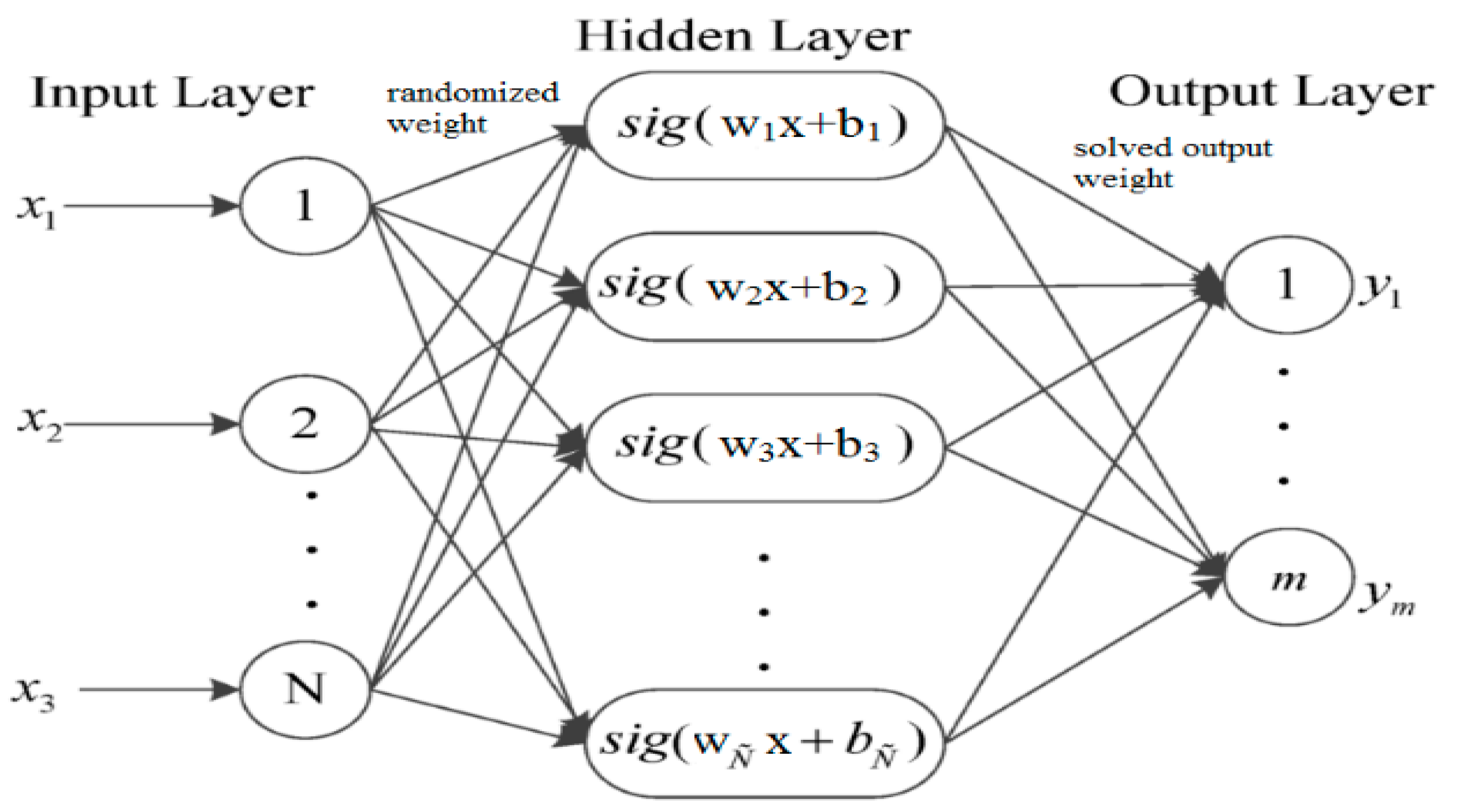
Instead of always estimating the SOC of each cell then determine the SOC for the pack, a single layer feedforward neural network (SLFN) trained by Extreme Learning Machine (ELM) is used. For n samples , where denotes the input, denotes the output with hidden neurons and sigmoid activation function a(x) = 1/(1 + e(−x)) as:
where is the weight vector connecting the i-th hidden neuron and input neurons, is the weight vector connecting the i-th hidden neuron and output neurons, and bi is the bias of the i-th hidden neuron. The aim of the ELM with hidden neurons with activation function a(x) can approximate the N samples with zero error, . Hence, there exist γi. w and bi so that:
Equation (8) can be written compactly as:
where H is called the hidden layer output matrix with the i-th column of H is the i-th hidden neuron’s output vector with respect to the input . Each neuron activation function is sigmoid in Figure 8.
In ELM, the input weight wi and bi will be randomly chosen. The output weights is analytically computed through the least square solution of a linear system:
where H† represents the Moore-Penrose generalized inverse of a matrix H. The results of the training can achieve a faster training, better generalization performance (i.e., small training error and smallest norm of output weights, avoid local minimal and do not need the activation function of the hidden neurons to be differentiable as compared to the gradient-based learning algorithm.
The term SOC(k) can be approximated using ELM learning. Equation (6) can be rewritten as:
Equation (14) can be expressed as equivalent form:
where: and is the parameter vector.
With measurement data where nt is the number of time measurements and the training set obtained, the SOC(k) can be written as:
where SOC(k) = [SOCk(2),SOCk(3),K,SOCk(ni)] and Hi = [Hi(1),Hi(2),K,Hi(ni − 1)]T.
By choosing the input weights and bias in the hidden layer nodes randomly, the parameter vector can be computed as:
Hence, the predicted SOC for the battery pack using the ELM learning can be written as follows:
The SOC will be first computed from the first set of data obtained from Section 2. Subsequently, the ELM learning will be used to train and predict the SOC of each cell in (16), followed by the SOC of the battery pack in (18). However, the data will arrive at certain sample time, i.e., 1 sample/s. The basic ELM may not be able to handle the sequential learning needs. As such, the adaptive online sequential ELM (AOS-ELM) will be used to learn the data batch-by-batch in a varying size. The next set of data will not be used until the learning is completed. The process of the AOS-ELM is as follows:
Step 1: Use a small batch of initial training data from the training set
Step 2: Assign random input weight wi and bi, .
Step 3: Compute the initially hidden layer output matrix, Hk:
Step 4: Estimate the initial output weight, where , .
Step 5: Set k = 0.
Step 6: For each i-th cell, compute where and
Step 7: Compute the total SOC for the battery pack, i.e., 12-cell i,j ∈ {1,K,Ns}.
Step 8: Provide (k + 1)-th batch of new observations as where Nk+1 denotes the number of observations in the (k + 1)-th batch.
Step 9: Compute the partial hidden layer output matrix Hk+1 for the (k + 1)-th batch of data Nk+1 as shown:
Step 10: Set target as
Step 11: Compute the output weight γ(k+1)
Step 12: Set k = k +1. Go to Step 6.
4. Performance Evaluation
First, there is a need to compare the performance of the ELM with the Ampere-hour method, Kalman filter-based methods (e.g., extended KF (EKF), strong tracking extended Kalman filter (STEKF), cubature Kalman filter (CKF), sliding-mode observer (SMO)) and other approaches such as backpropagation (BP) and radial basis function (RBF). Second, different ELM-based methods such as bidirectional-ELM (B-ELM), incremental-ELM (I-ELM), parallel chaos search ELM (P-ELM) and online-sequential ELM (OS-ELM) will be compared with the proposed adaptive online-sequential ELM (AOS-ELM) across a single cell at different ambient temperature. The SOC for the battery pack will then be obtained at 25 °C.
4.1. Comparison between ELM and Kalman Filter-Based Methods
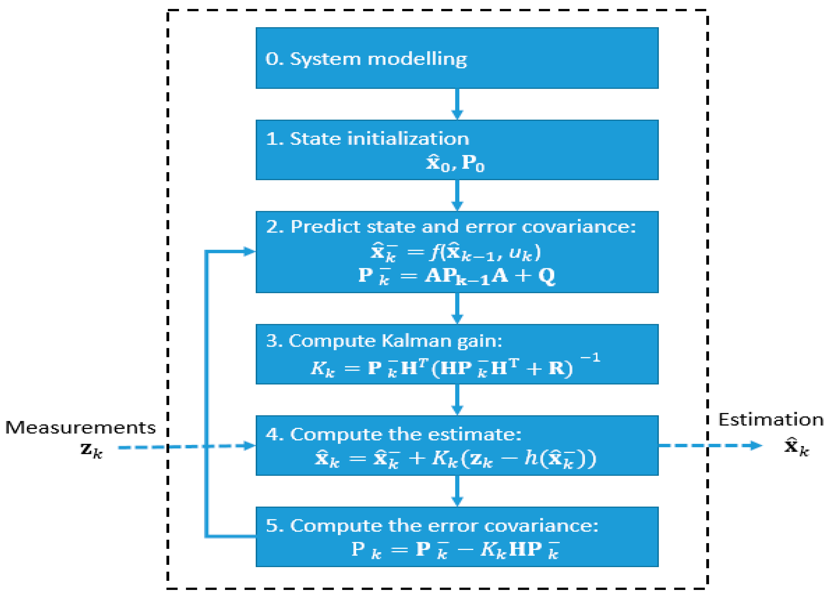
The Extended Kalman Filter (EKF) can be used to estimate the SOC of the discrete-time nonlinear battery model. The traditional computation flowchart for EKF can be seen in Figure 9. The strong tracking filter (STF) [68] with online adaptively modified Kalman gain matrix and prior state error covariance to track the sudden change in the state vectors was also used. The critical feature of the STF is the method to rearrange the prior error covariance by multiplying it by a diagonal matrix in which the differing diagonal entries optimize the propagation of components in state vector by diminishing the impacts of old data on current parameter estimation:
where denotes multiple fading factors matrix that is determined as:
where the proportion of and its constraint can be determined by prior knowledge of the system.
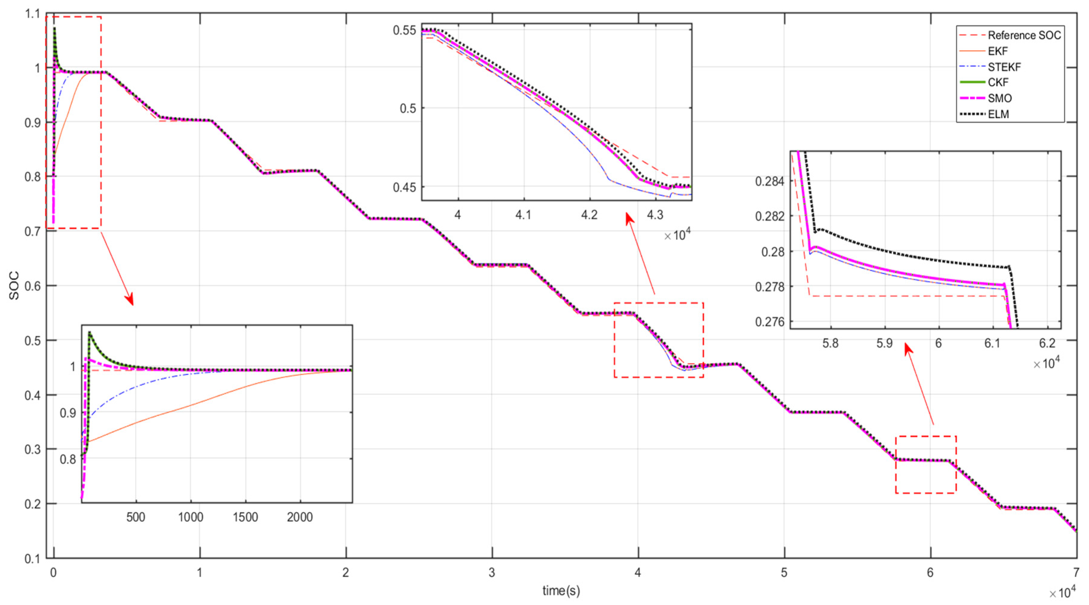
The STEKF was then developed by applying the strong tracking algorithm on the EKF. STEKF benefits the estimation process by taking the advantages of EKF that minimizes the estimation error covariance and STF that tracks the state vector variation accurately. On the other hand, the cubature Kalman filter generates a set of cubature points propagated by system equations to approximate the posterior estimate was used. It can also track the fast-changing SOC value. A different numbers of hidden nodes were chosen and the corresponding results were tabulated in Table 7. The results show that the ELM with 10 neurons and sigmoid activation function are faster and produces lower RSME as compared to EKF, STEKF, CKF and SMO. The RSME was computed using the Ampere-hour method as the reference.
By comparing the EKF-based methods with ELM, the RMSE has the lowest computational time. Table 7 shows that ELM is a viable method to model and predict the SOC value for the given current, voltage and capacity. As shown in Figure 10, the SMO shows a better fit during the initial stage of SOC estimation as compared to other EKF methods. On the other hand, the ELM exhibits an overshoot but settle to steady state quickly during the initial stage of estimation. The spike was caused by a transient at initial prediction. Nevertheless, ELM method performs better as the charging and discharging cycle increase. As a result, the ELM based approach will be used for the SOC estimation of the battery cell in the next section.
4.2. Comparison between ELM and Non-ELM Based Approaches
The performance of the ELM will be compared with some common methods such as the BP and RBF. It is followed by comparing the proposed adaptive online sequential learning algorithm with the ELM, B-ELM, I-ELM, OS-ELM, and P-ELM [48] at different ambient temperatures. The details of how these learning algorithms work can be found in the various references cited in this paper. For brevity, the detailed working principles of the algorithms are not shown here. MATLAB was used for all the machine learning running on an Intel® Core i7-5500u CPU (2.4 GHz) equipped with 16 GB of RAM. Each neuron activation function can be sinusoidal, radial basis function and sigmoidal. In this paper, the sigmoid activation function was used for BP, RBF and ELM. A different number of hidden nodes will be chosen and the corresponding results for testing RMSE and training time are tabulated. The training data constitute 70% of the total dataset and the remaining 30% data are used for testing the trained model.
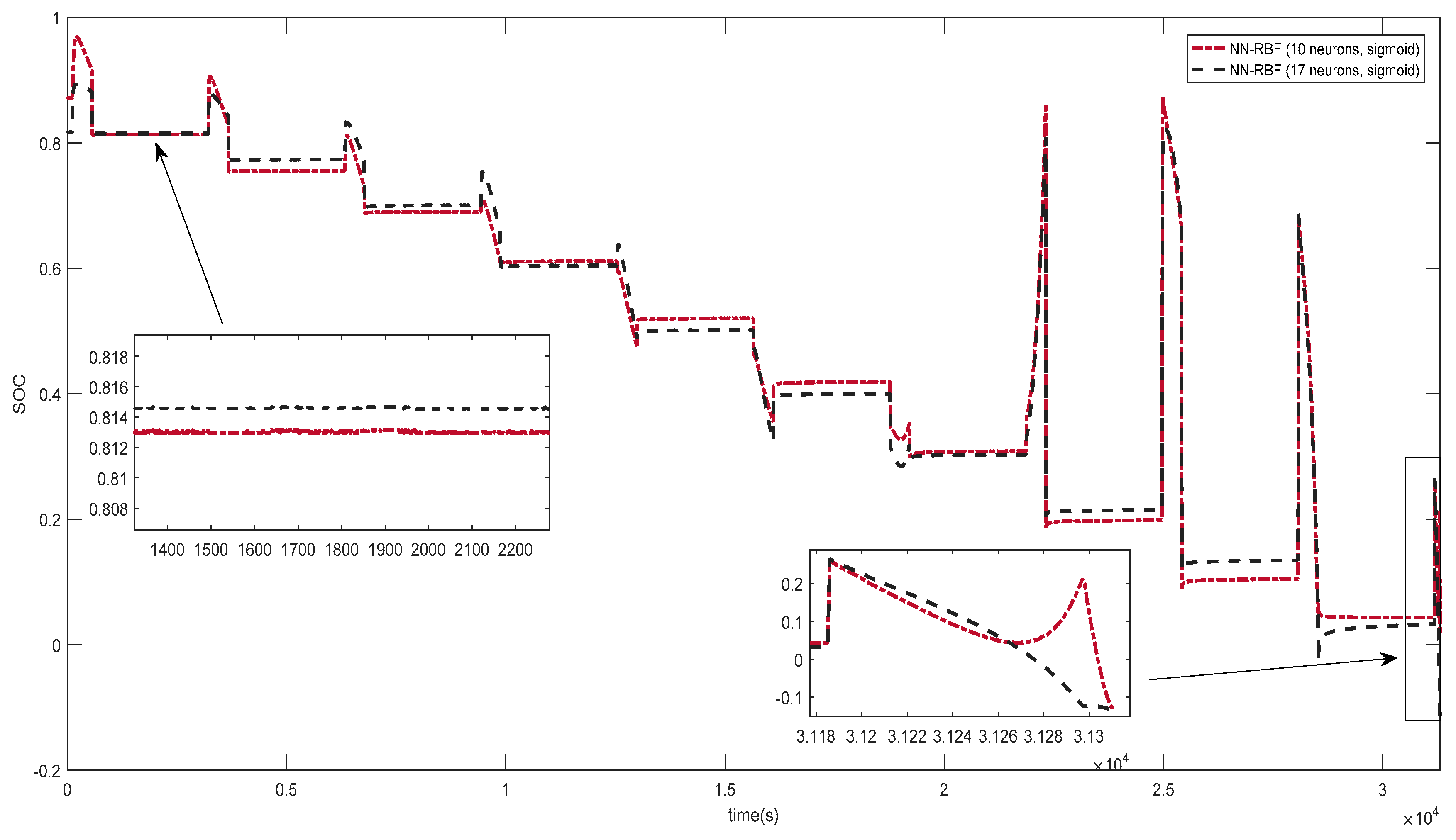
In the backpropagation algorithm, a forward propagation was used to compute all the sigmoid activations throughout the network using initial random weights and constant bias term in layer 1 and 2, including the output value. The sigmoid activation has the least RMSE as compared to sinusoidal function. The learning rate is set to 1 with three input neurons (current, voltage, and capacity (in Ah)), one output (SOC value) with a different number of hidden neurons. The results of the training using backpropagation algorithm can be seen in Table 8. The SOC comparison using the same number of neurons can be seen in Figure 11. In BP, the maximum root mean squared error (RMSE) of the testing data set for SOC is approximately 2.454. The CPU training time incurred during the training is not more than 4066 s. With 17 neurons, the RMSE increased to 4.879 with a training time of 1952 s.
In the case of RBF, it gives RMSE of 0.1 at a lower CPU training time of 417.6 s. As compared to ELM with 10 neurons, the RMSE is 0.0004 under the training time of 0.031 s. The SOC plots for basic ELM, BP and RBF can be seen in Figure 12, Figure 13 and Figure 14, respectively. However, as compared to the case of 5 neurons for ELM, the RMSE is 0.0178 and the training time is 0.00001 s. The RMSE reduced by 97% at a faster training time as compared to the case of 10 neurons.
In summary, the extreme learning machine gives a lower training time and reasonable RMSE as compared to BP and RBF. With only five hidden neurons and a sigmoid activation function used in ELM, it can achieve the same or better performance than RBF and BP (that used 10 or more neurons). Further increases in the hidden neurons in ELM will result in a lower testing RMSE with a more prolonged training time.
4.3. Comparison between ELM and Other ELM Based Approaches
In addition to the basic ELM, other types of ELM such as B-ELM, I-ELM, P-ELM, OS-ELM and AOS-ELM will be compared at different ambient temperatures. As shown in Section 4.2, ELM exhibits a faster training time and smaller testing RMSE with only five neurons as compared to BP and RBF. The ELM gives a less complex neural network architecture as fewer neurons can be used. With a higher number of hidden nodes, the testing RMSE can be reduced. For each ambient temperature, the average results of 10 trials for ELM based approaches can be obtained. During the training process, ELM based approaches were given a different number of hidden nodes to examine the effect of increasing the hidden nodes (or increase in network complexity).
In summary, the improved version of I-ELM named B-ELM has a shorter training time than I-ELM with a similar testing RMSE. The same trend of linearly increasing in the training time as some neuron increases can be observed. With less hidden nodes, it gives faster training time. The ELM and B-ELM with only five hidden nodes across different ambient temperatures can achieve similar results for I-ELM that uses 20 hidden nodes. Hence, B-ELM performs better than I-ELM.
In parallel chaos search-based ELM (P-ELM), at each learning step, optimal hidden nodes selected by the parallel chaos optimization algorithm are added to the current network to minimize the error between target and network output. Increasing the number of hidden nodes improves the testing RMSE but increases the training time. The P-ELM performs better in both the training time and testing RMSE than I-ELM for a higher number of the neuron. However, it does not outperform the B-ELM at 5 and 10 hidden nodes at each temperature. A similar result for P-ELM that uses 20 hidden nodes is unable to perform better than B-ELM with only five hidden nodes.
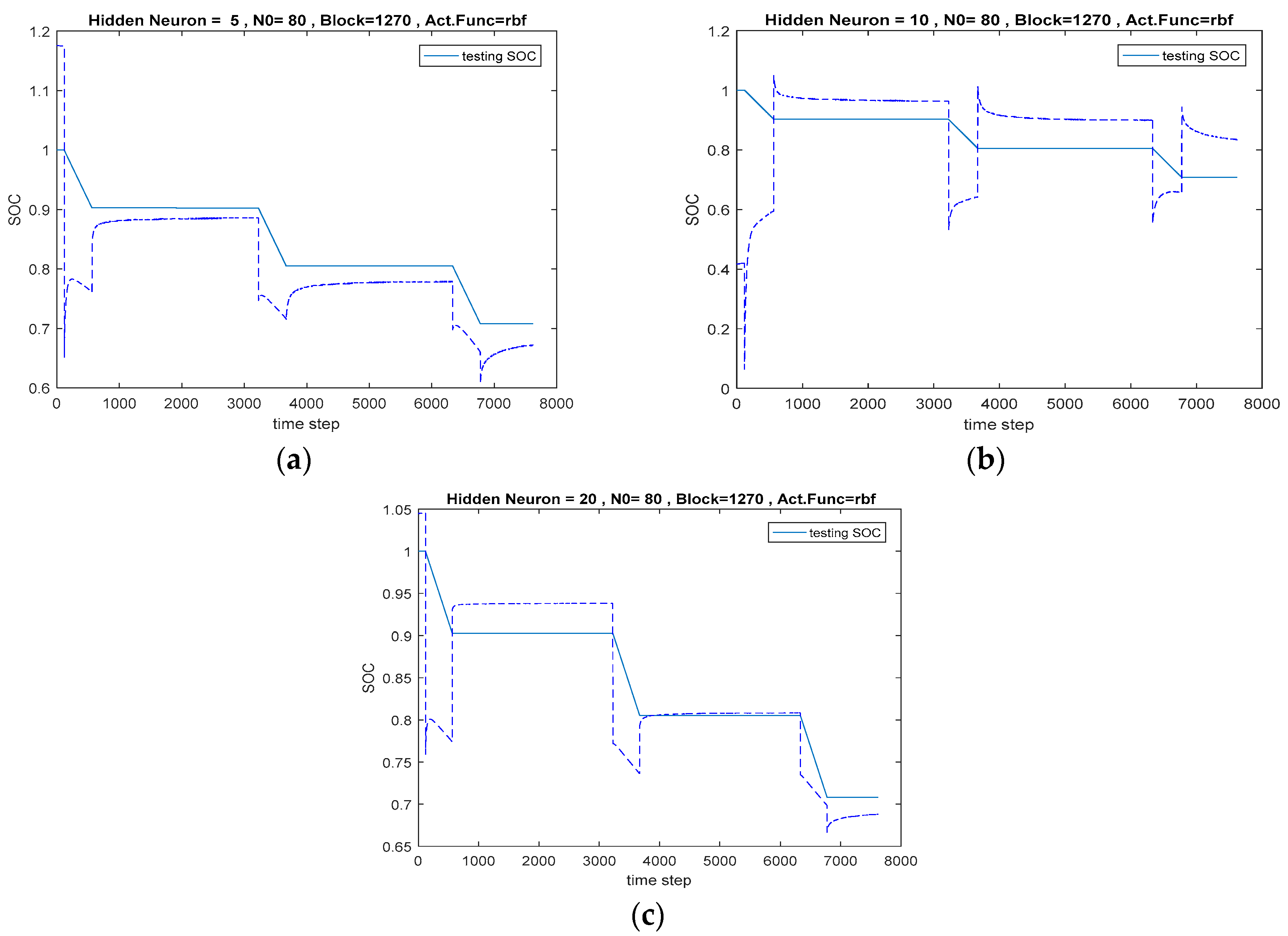
In contrast to I-ELM, B-ELM, and P-ELM, the testing RMSE for OS-ELM is lower (except for neuron equals to 20) in Table 9. The number of initial training data used in the preliminary phase of OS-ELM and the size of the block of data learned by OS-ELM in each step can vary for different ambient temperatures as seen in Table 9. The initial number of training data is not more than 590. This number is far less than the entire dataset (approximately 30,000) used for the training and testing. The training time is longer than I-ELM and B-ELM but shorter than P-ELM. The training time is not dependent on the number of neurons as seen in Table 9. The testing RMSE is quite constant throughout the number of neurons. The SOC testing performance of online sequential ELM at 25 °C ambient temperature for different neuron can be seen in Figure 15. It can be observed that the SOC performance does not improved with the number of neurons.
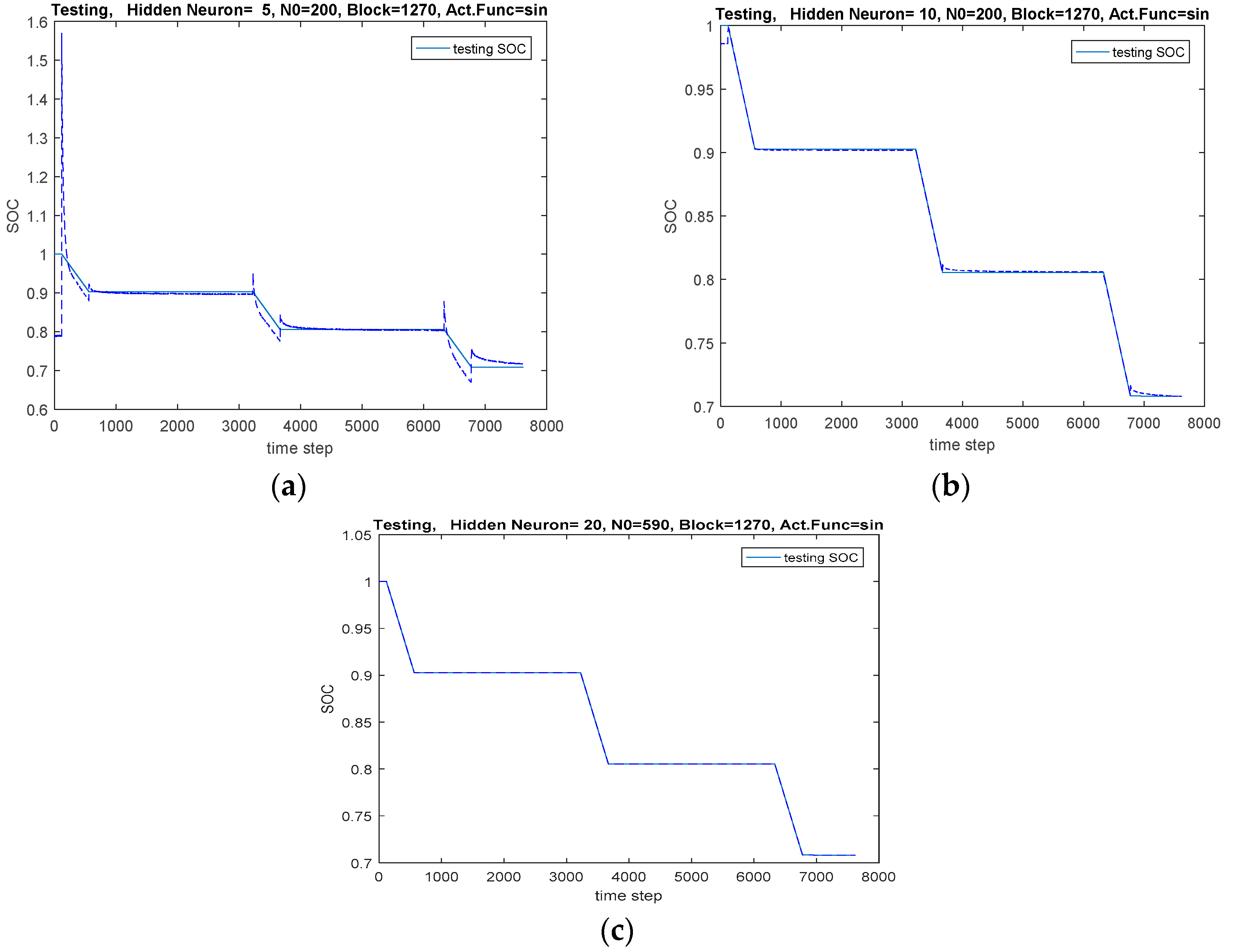
The adaptive version of OS-ELM named AOS-ELM produces a lower testing RMSE and reasonable training time (Table 10). In addition, the testing RMSE and training time are smaller than the basic ELM, I-ELM, B-ELM and P-ELM. However, as the number of neuron increases in the basic ELM, it performs better at the expense of a higher network complexity. The testing RMSE of AOS-ELM is smaller than OS-ELM as the size of data block randomly generated in each iteration of sequential learning phase can be adjusted across different ambient temperatures. As shown in Table 10, the AOS-ELM with five neurons has the smallest testing RMSE as compared to 10 and 20 neurons. Hence, the complexity of the neural networks can be reduced. In addition, the number of initial training data used in the initial phase (N0) in AOS-ELM will need to increase to obtain a smaller testing RMSE. The similar phenomena can be seen in the SOC response depicted in Figure 16. Note that the value should not increase the size of the entire dataset to resemble other non-sequential methods.
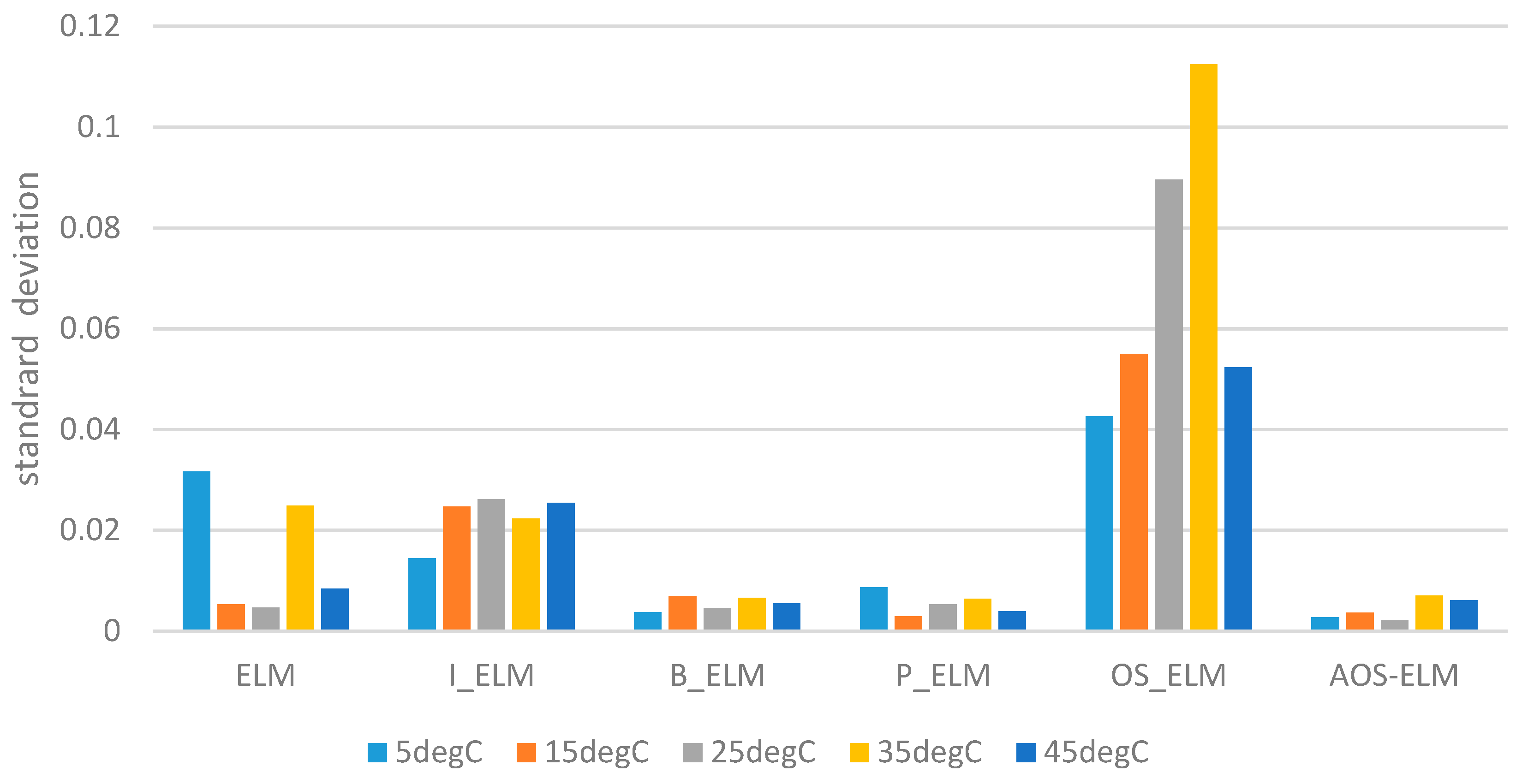
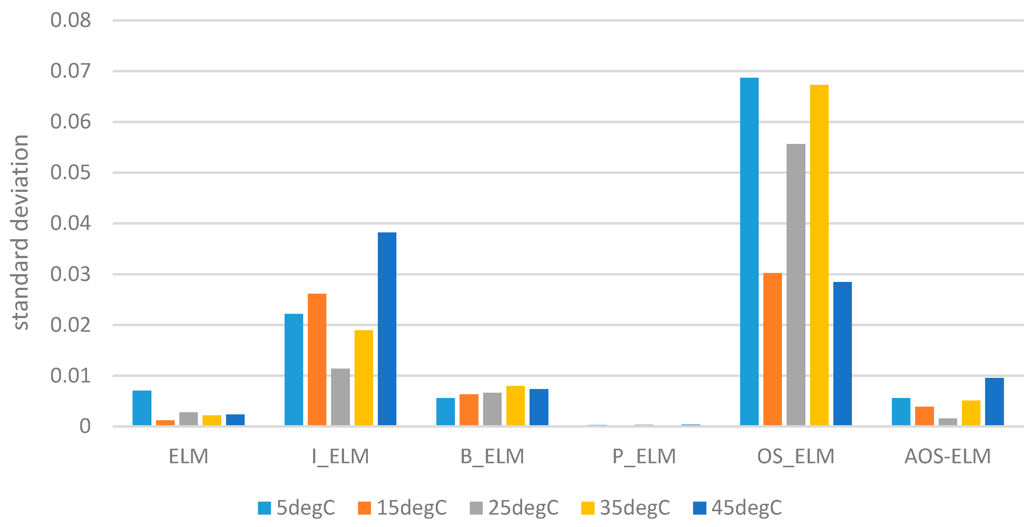
Besides using the absolute value obtained for the training time and testing RMSE, it is important to examine the standard deviation due to the random initialization of weights used in ELM. In each ambient temperature, the standard deviation of 10 trials was obtained for five, 10 and 20 neurons, respectively. The same parameters will be used. As shown in Figure 17, Figure 18 and Figure 19, the results show the fluctuation of the ELM based learning after multiple simulations using the same settings for each method. The OS-ELM has the highest standard deviation as compared to the rest. Conversely, P-ELM produces the lowest standard deviation followed by B-ELM and ELM and I-ELM. The results show that AOS-ELM gives a reasonable standard deviation at five and 10 neurons as compared to OS-ELM, I-ELM and basic ELM. It indicates that AOS-ELM is less complicated in the neural network and gives a faster computation time with more consistency with the results than OS-ELM.
In summary, AOS-ELM provides some robustness to the learning outcome at different ambient temperatures. By increasing the number of initial training data used (N0 = 200) and decreasing the range of the size of the data block (Block_Range = 847), it improves the testing RMSE as shown (see Table 11). The initial number of training data is smaller than the entire dataset for the training and testing. With smaller RMSE, it implies that the standard deviation will be smaller. In addition, with the gradual increase in the dataset obtained during the initial stage of the training that can be adaptively adjusted using N0, AOS-ELM is more suitable to estimate the SOC for the 12-cell battery.
4.4. Performance of SOC for 12-Cell Using AOS-ELM
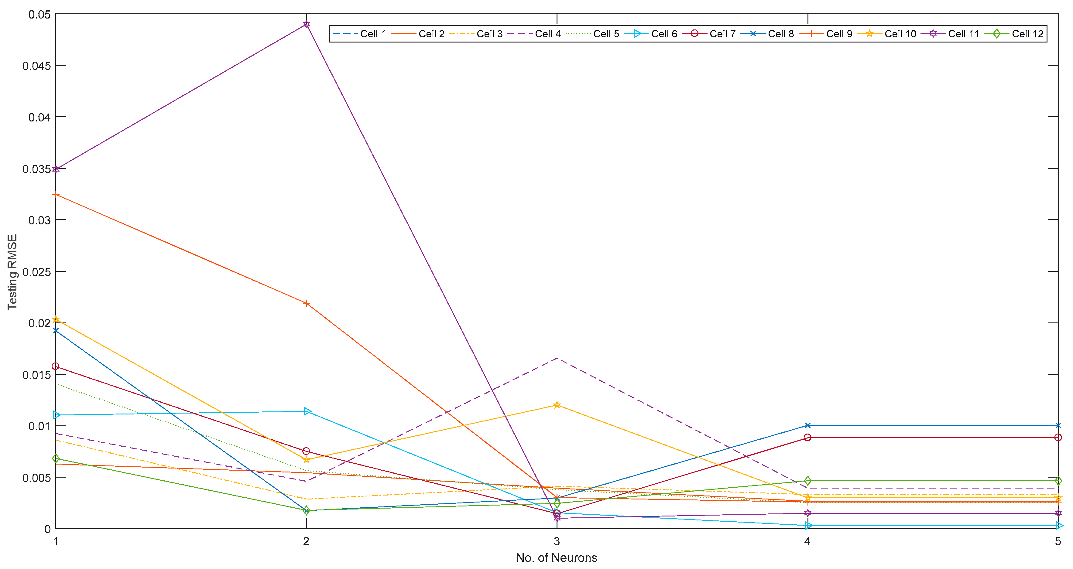
The use of AOS-ELM for the case of a 12-cell battery will be examined. For brevity, the ambient temperature at 25 °C will be examined. A similar approach can be applied to other ambient temperatures. As shown in Figure 20, the testing RMSE converges to the steady-state in five neurons. It shows the least error as compared to a lower number of neurons. Since a smaller number of neurons provide the same or slightly better performance in training time and testing RMSE, the five neurons will be used for all the AOS-ELM learning. The training time (see Figure 21) increases as the number of neuron increases. Note that the testing RMSE differs among the 12 cells in Figure 22. The training time is quite constant across the 12-cell. The testing RMSE across the 12-cell is around 0.002157 (as indicated as a dotted line in Figure 22). The RMSE is quite small to show that cell balancing may not be required for the 12 cells as the performance of each cell does not differ too much.
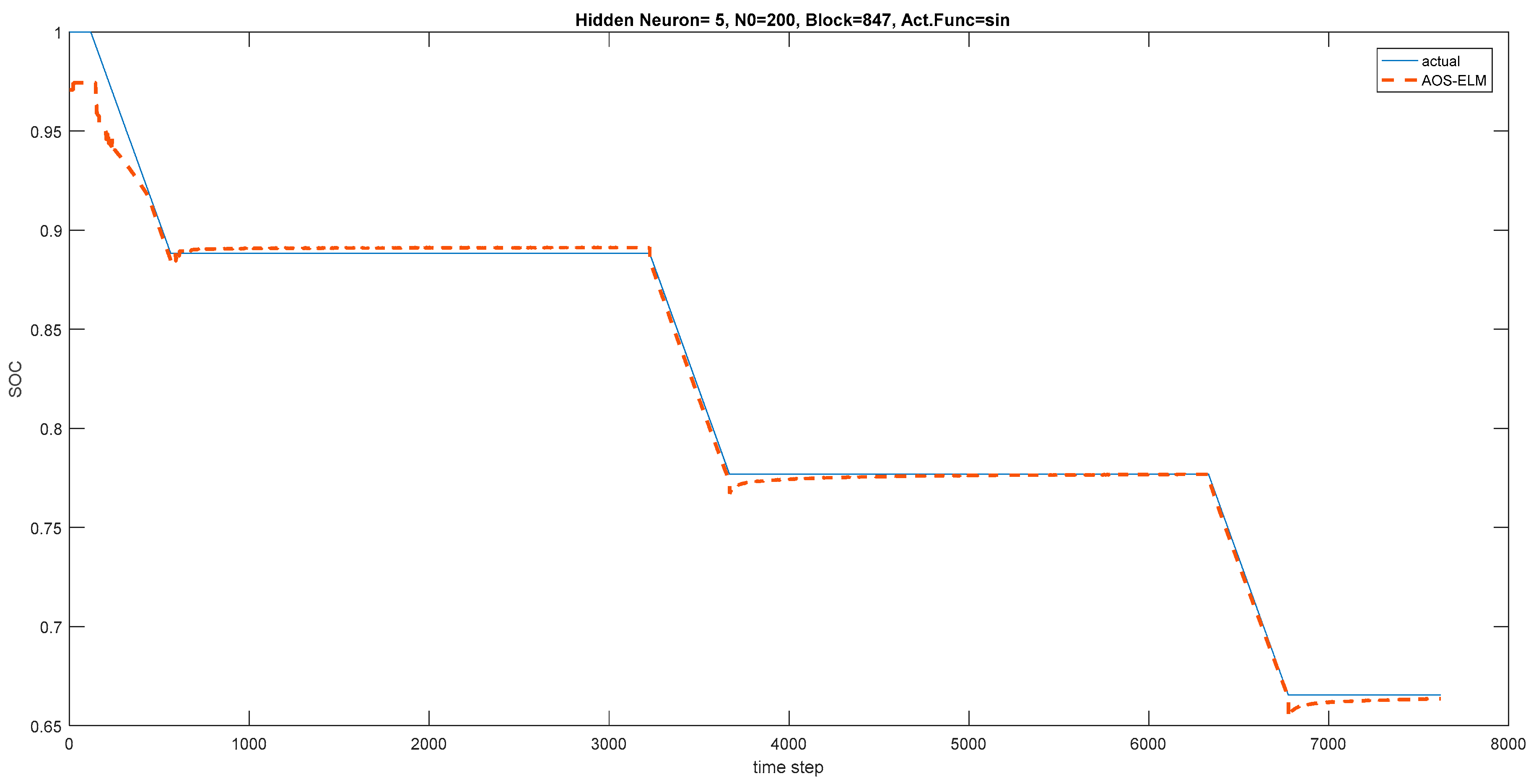
In summary, AOS-ELM gives a lower testing RMSE at a higher number of neurons but with a longer training time and complexity in the neural networks as compared to OS-ELM, B-ELM and basic ELM. Although the P-ELM has the lowest standard deviation, it has the longest training time as compared to AOS-ELM and other methods. As shown in Figure 23, the pack SOC from AOS-ELM (0.8172) is quite close to the actual SOC (0.8167) obtained from the Ampere-hour method. The pack SOC using the proposed AOS-ELM can, therefore, predict the SOC of the 12-cell with lower and better consistency in the testing RMSE and shorter training time.
5. Conclusions
This paper has proposed the state-of-charge (SOC) estimation of battery power systems using an adaptive online sequential extreme learning machine (AOS-ELM). The SOC value of battery cells is influenced by many uncertain parameters such as the model and ambient temperature. The proposed AOS-ELM method for SOC estimation is useful where the input data such as current, voltage, capacity are progressively available in batches with small sample size from the cells in the early training stage. As compared to other approaches such as extended Kalman filter (EKF)-based approaches, the ELM-based learning produced faster computational time with lower root mean square error (RMSE). As shown in the comparisons with the bidirectional-ELM (B-ELM), incremental-ELM (I-ELM), parallel-chaos search-based incremental ELM (P-ELM), online sequential ELM (OS-ELM), the AOS-ELM produced lower testing RMSE and reasonable training time. The testing RMSE and its standard deviation of the AOS-ELM could be smaller than the OS-ELM, and other approaches as the size of data block were randomly generated and adjusted in each iteration of the sequential learning phase. As a result, the pack SOC value obtained from AOS-ELM could estimate a SOC of the 12-cell battery close to the value determined by the Ampere-hour method. The subsequent calibration of the cells’ static capacity and equivalent circuit models of the battery cells were not required as the AOS-ELM could be used to estimate the SOC. For future works, the proposed AOS-ELM model will be further optimized and improved. Other different types of deep neural network will be analyzed and compared. More works will be performed to improve the AOS-ELM learning algorithm for multi-cell modeling under varying operating parameters.
Acknowledgments
The authors would like to thank Newcastle University and Temasek Polytechnic for providing research supports.
Author Contributions
Zuchang Gao is credited with the majority of the battery model formulation, validation and experimental works performed in this paper for his PhD study. Cheng Siong Chin who is the main supervisor defined the flow of the paper and performed the machine learning simulation, paper writing and comparisons of ELM and non-ELM approaches that drove this research.
Conflicts of Interest
The authors declare no conflict of interest.
References
- Zhang, Y.; Zhang, C.; Zhang, X. State-of-charge estimation of the lithium-ion battery system with a time-varying parameter for hybrid electric vehicles. IET Control Theory Appl. 2014, 8, 160–167. [Google Scholar] [CrossRef]
- Alhanouti, M.; Gießler, M.; Blank, T.; Gauterin, F. New Electro-Thermal Battery Pack Model of an Electric Vehicle. Energies 2016, 9, 563. [Google Scholar] [CrossRef]
- Hussein, A.A. Capacity Fade Estimation in Electric Vehicle Li-Ion Batteries Using Artificial Neural Networks. IEEE Trans. Ind. Appl. 2015, 51, 2321–2330. [Google Scholar] [CrossRef]
- Tenfen, D.; Finardi, E.C.; Delinchant, B.; Wurtz, F. Lithium-ion battery modeling for the energy management problem of microgrids. IET Gener. Transm. Distrib. 2016, 10, 576–584. [Google Scholar] [CrossRef]
- Ye, F.; Qian, Y.; Hu, R.Q. Incentive Load Scheduling Schemes for PHEV Battery Exchange Stations in Smart Grid. IEEE Syst. J. 2017, 11, 922–930. [Google Scholar] [CrossRef]
- Casals, L.C.; Garca, B.A. Communications concerns for reused electric vehicle batteries in smart grids. IEEE Commun. Mag. 2016, 54, 120–125. [Google Scholar] [CrossRef] [Green Version]
- Chaturvedi, N.A.; Klein, R.; Christensen, J.; Ahmed, J.; Kojic, A. Algorithms for advanced battery-management systems. IEEE Control Syst. 2010, 30, 49–68. [Google Scholar] [CrossRef]
- Pop, V.; Bergveld, H.J.; Notten, P.H.L.; Regtien, P.P.L. State of-the-art of battery state-of-charge determination. Meas. Sci. Technol. 2005, 16, R93–R110. [Google Scholar] [CrossRef]
- Newman, J.; Thomas-Aleya, K.E. Electrochemical Systems, 4th ed.; Wiley: Hoboken, NJ, USA, 2004. [Google Scholar]
- Botte, G.G.; Subramanian, V.R.; White, R.E. Mathematical modeling of secondary lithium batteries. Electrochim. Acta 2000, 45, 2595–2609. [Google Scholar] [CrossRef]
- Hu, Y.; Yurkovich, S.; Guezennec, Y.; Yurkovich, B.J. Electro-thermal battery model identification for automotive applications. J. Power Sources 2011, 196, 449–457. [Google Scholar] [CrossRef]
- Sung, W.; Shin, C.B. Electrochemical model of a lithium-ion battery implemented into an automotive battery management system. Comput. Chem. Eng. 2015, 76, 87–97. [Google Scholar] [CrossRef]
- Hu, X.S.; Cao, D.P.; Egardt, B. Condition Monitoring in Advanced Battery Management Systems: Moving Horizon Estimation Using a Reduced Electrochemical Model. IEEE/ASME Trans. Mechatron. 2018, 23, 167–178. [Google Scholar] [CrossRef]
- Zhao, S.; Duncan, S.R.; Howey, D.A. Observability Analysis and State Estimation of Lithium-Ion Batteries in the Presence of Sensor Biases. IEEE Trans. Control Syst. Technol. 2017, 25, 326–333. [Google Scholar] [CrossRef]
- Plett, G.L. Extended Kalman filtering for battery management systems of LiPB-based HEV battery packs: Part 3. State and parameter estimation. J. Power Sources 2004, 134, 277–292. [Google Scholar] [CrossRef]
- Plett, G.L. Sigma-point Kalman filtering for battery management systems of LiPB-based HEV battery packs: Part 2: Simultaneous state and parameter estimation. J. Power Sources 2006, 161, 1369–1384. [Google Scholar] [CrossRef]
- Kim, I.-M. The novel state of charge estimation method for lithium battery using sliding mode observer. J. Power Sources 2006, 163, 584–590. [Google Scholar] [CrossRef]
- Verbrugge, M.; Tate, E. Adaptive state of charge algorithm for nickel metal hydride batteries including hysteresis phenomena. J. Power Sources 2004, 126, 236–249. [Google Scholar] [CrossRef]
- Hu, Y.; Yurkovich, S. Battery cell state-of-charge estimation using linear parameter varying system techniques. J. Power Sources 2012, 198, 338–350. [Google Scholar] [CrossRef]
- Di Domenico, D.; Fiengo, G.; Stefanopoulou, A. Lithium-ion battery state of charge estimation with a Kalman filter based on a electrochemical model. In Proceedings of the IEEE International Conference on Control Applications, San Antonio, TX, USA, 3–5 September 2008; pp. 702–707. [Google Scholar]
- Santhanagopalan, S.; White, R.E. State of charge estimation using an unscented filter for high power lithium ion cells. Int. J. Energy Res. 2010, 34, 152–163. [Google Scholar] [CrossRef]
- Klein, R.; Chaturvedi, N.A.; Christensen, J.; Ahmed, J.; Findeisen, R.; Kojic, A. Electrochemical model based observer design for a lithium-ion battery. IEEE Trans. Control Syst. Technol. 2013, 21, 289–301. [Google Scholar] [CrossRef]
- Jia, J.; Lin, P.; Chin, C.S.; Toh, W.D.; Gao, Z.; Lyu, H.; Cham, Y.T.; Mesbahi, E. Multirate strong tracking extended Kalman filter and its implementation on lithium iron phosphate (LiFePO4) battery system. In Proceedings of the IEEE 11th International Conference on Power Electronics and Drive Systems, Sydney, Australia, 9–12 June 2015; pp. 640–645. [Google Scholar]
- Li, W.; Shah, S.L.; Xiao, D. Kalman filters in nonuniformly sampled multirate systems: For FDI and beyond. Automatica 2008, 44, 199–208. [Google Scholar] [CrossRef]
- Arasaratnam, I.; Haykin, S. Cubature Kalman Filters. IEEE Trans. Autom. Control 2009, 54, 1254–1269. [Google Scholar] [CrossRef]
- Wang, D.; Yang, F.; Tsui, K.L.; Zhou, Q.; Bae, S.J. Remaining Useful Life Prediction of Lithium-Ion Batteries Based on Spherical Cubature Particle Filter. IEEE Trans. Instrum. Meas. 2016, 65, 1282–1291. [Google Scholar] [CrossRef]
- Li, I.H.; Wang, W.Y.; Su, S.F.; Lee, Y.S. A Merged Fuzzy Neural Network and Its Applications in Battery State-of-Charge Estimation. IEEE Trans. Energy Convers. 2007, 22, 697–708. [Google Scholar] [CrossRef]
- Charkhgard, M.; Farrokhi, M. State-of-Charge Estimation for Lithium-Ion Batteries Using Neural Networks and Ekf. IEEE Trans. Ind. Electron. 2010, 57, 4178–4187. [Google Scholar] [CrossRef]
- He, W.; Williard, N.; Chen, C.; Pecht, M. State of Charge Estimation for Li-Ion Batteries Using Neural Network Modeling and Unscented Kalman Filter-Based Error Cancellation. Int. J. Electr. Power Energy Syst. 2014, 62, 783–791. [Google Scholar] [CrossRef]
- Wang, S.C.; Liu, Y.H. A Pso-Based Fuzzy-Controlled Searching for the Optimal Charge Pattern of Li-Ion Batteries. IEEE Trans. Ind. Electron. 2015, 62, 2983–2993. [Google Scholar] [CrossRef]
- Melin, P.; Castillo, O. Intelligent Control of Complex Electrochemical Systems with a Neuro-Fuzzy-Genetic Approach. IEEE Trans. Ind. Electron. 2001, 48, 951–955. [Google Scholar] [CrossRef]
- Hu, X.; Li, S.E.; Yang, Y. Advanced Machine Learning Approach for Lithium-Ion Battery State Estimation in Electric Vehicles. IEEE Trans. Transp. Electr. 2016, 2, 140–149. [Google Scholar] [CrossRef]
- Weng, C.; Cui, Y.; Sun, J.; Peng, H. On-board state of health monitoring of lithium-ion batteries using incremental capacity analysis wit support vector regression. J. Power Sources 2013, 235, 36–44. [Google Scholar] [CrossRef]
- Huang, G.B.; Zhou, H.; Ding, X.; Zhang, R. Extreme learning machine for regression and multiclass classification. IEEE Trans. Syst. Man Cybern. B Cybern. 2012, 42, 513–529. [Google Scholar] [CrossRef] [PubMed]
- Rumelhart, D.E.; Hinton, G.E.; Williams, R.J. Learning representations by back-propagating errors. Nature 1986, 323, 533–536. [Google Scholar] [CrossRef]
- Huang, G.-B.; Chen, L.; Siew, C.-K. Universal approximation using incremental constructive feedforward networks with random hidden nodes. IEEE Trans. Neural Netw. 2006, 17, 879–892. [Google Scholar] [CrossRef] [PubMed]
- Huang, G.-B.; Li, M.-B.; Chen, L.; Siew, C.-K. Incremental extreme learning machine with fully complex hidden nodes. Neurocomputing 2008, 71, 576–583. [Google Scholar] [CrossRef]
- Huang, G.-B. An insight into extreme learning machines: Random neurons, random features and kernels. Cognit. Comput. 2014, 6, 376–390. [Google Scholar] [CrossRef]
- Ferrari, S.; Stengel, R.F. Smooth function approximation using neural networks. IEEE Trans. Neural Netw. 2005, 16, 24–38. [Google Scholar] [CrossRef] [PubMed]
- Xiang, C.; Ding, S.Q.; Lee, T.H. Geometrical interpretation and architecture selection of {MLP}. IEEE Trans. Neural Netw. 2005, 16, 84–96. [Google Scholar] [CrossRef] [PubMed]
- Huang, G.-B.; Babri, H.A. Upper bounds on the number of hidden neurons in feedforward networks with arbitrary bounded nonlinear activation functions. IEEE Trans. Neural Netw. 1998, 9, 224–229. [Google Scholar] [CrossRef] [PubMed]
- Huang, G.-B.; Chen, Y.-Q.; Babri, H.A. Classification ability of single hidden layer feedforward neural networks. IEEE Trans. Neural Netw. 2000, 11, 799–801. [Google Scholar] [CrossRef] [PubMed]
- Mao, K.Z.; Huang, G.-B. Neuron selection for RBF neural network classifier based on data structure preserving criterion. IEEE Trans. Neural Netw. 2005, 16, 1531–1540. [Google Scholar] [CrossRef] [PubMed]
- Park, J.; Sandberg, I.W. Universal approximation using radial basis-function networks. Neural Comput. 1991, 3, 246–257. [Google Scholar] [CrossRef]
- Leshno, M.; Lin, V.Y.; Pinkus, A.; Schocken, S. Multilayer feedforward networks with a nonpolynomial activation function can approximate any function. Neural Netw. 1993, 6, 861–867. [Google Scholar] [CrossRef]
- Kwok, T.-Y.; Yeung, D.-Y. Objective functions for training new hidden units in constructive neural networks. IEEE Trans. Neural Netw. 1997, 8, 1131–1148. [Google Scholar] [CrossRef] [PubMed]
- Meir, R.; Maiorov, V.E. On the optimality of neural-network approximation using incremental algorithms. IEEE Trans. Neural Netw. 2000, 11, 323–337. [Google Scholar] [CrossRef] [PubMed]
- Liang, N.; Huang, G.; Saratchandran, P.; Sundararajan, N. A Fast and Accurate Online Sequential Learning Algorithm for Feedforward Networks. IEEE Trans. Neural Netw. 2006, 17, 1411–1423. [Google Scholar] [CrossRef] [PubMed]
- Tang, J.; Deng, C.; Huang, G. Extreme Learning Machine for Multilayer Perceptron. IEEE Trans. Neural Netw. Learn. Syst. 2016, 27, 809–821. [Google Scholar] [CrossRef] [PubMed]
- Huang, G.-B.; Chen, L. Convex incremental extreme learning machine. Neurocomputing 2007, 70, 3056–3062. [Google Scholar] [CrossRef]
- Huang, G.-B.; Chen, L. Enhanced random search based incremental extreme learning machine. Neurocomputing 2008, 71, 3460–3468. [Google Scholar] [CrossRef]
- Feng, G.; Huang, G.B.; Lin, Q.; Gay, R. Error minimized extreme learning machine with growth of hidden nodes and incremental learning. IEEE Trans. Neural Netw. 2009, 20, 1352–1357. [Google Scholar] [CrossRef] [PubMed]
- Miche, Y.; Sorjamaa, A.; Bas, P.; Simula, O.; Jutten, C.; Lendasse, A. OP-ELM: Optimally pruned extreme learning machine. IEEE Trans. Neural Netw. 2010, 21, 158–162. [Google Scholar] [CrossRef] [PubMed]
- Yang, Y.; Wang, Y.; Yuan, X. Bidirectional Extreme Learning Machine for Regression Problem and Its Learning Effectiveness. IEEE Trans. Neural Netw. 2012, 23, 1498–1505. [Google Scholar] [CrossRef] [PubMed]
- Platt, J. A resource-allocating network for function interpolation. Neural Comput. 1991, 3, 213–225. [Google Scholar] [CrossRef]
- Kadirkamanathan, V.; Niranjan, M. A function estimation approach to sequential learning with neural networks. Neural Comput. 1993, 5, 954–975. [Google Scholar] [CrossRef]
- Yingwei, L.; Sundararajan, N.; Saratchandran, P. A sequential learning scheme for function approximation using minimal radial basis function (RBF) neural networks. Neural Comput. 1997, 9, 461–478. [Google Scholar] [CrossRef]
- Yingwei, L.; Sundararajan, N.; Saratchandran, P. Performance evaluation of a sequental minimal radial basis function (RBF) neural network learning algorithm. IEEE Trans. Neural Netw. 1998, 9, 308–318. [Google Scholar] [CrossRef] [PubMed]
- Huang, G.-B.; Saratchandran, P.; Sundararajan, N. An efficient sequential learning algorithm for growing and pruning RBF (GAP-RBF) networks. IEEE Trans. Syst. Man Cybern. B Cybern. 2004, 34, 2284–2292. [Google Scholar] [CrossRef] [PubMed]
- Huang, G.-B.; Saratchandran, P.; Sundararajan, N. A generalized growing and pruning RBF (GGAP-RBF) neural network for function approximation. IEEE Trans. Neural Netw. 2005, 16, 57–67. [Google Scholar] [CrossRef] [PubMed]
- Huang, G.-B.; Zhu, Q.-Y.; Siew, C.-K. Extreme learning machine: A new learning scheme of feedforward neural networks. In Proceedings of the International Joint Conference on Neural Network (IJCNN2004), Budapest, Hungary, 25–29 July 2004; Volume 2, pp. 985–990. [Google Scholar]
- Huang, G.-B.; Siew, C.-K. Extreme learning machine: RBF network case. In Proceedings of the 8th International Conference on Control, Automation, Robotics and Vision (ICARCV 2004), Kunming, China, 6–9 December 2004; Volume 2, pp. 1029–1036. [Google Scholar]
- Huang, G.-B.; Zhu, Q.-Y.; Mao, K.Z.; Siew, C.-K.; Saratchandran, P.; Sundararajan, N. Can threshold networks be trained directly? IEEE Trans. Circuits Syst. II Exp. Briefs 2006, 53, 187–191. [Google Scholar] [CrossRef]
- Huang, G.-B.; Zhu, Q.-Y.; Siew, C.-K. Extreme learning machine: Theory and applications. Neurocomput 2006, 70, 489–501. [Google Scholar] [CrossRef]
- Li, G.; Liu, M.; Dong, M. A new online learning algorithm for structure-adjustable extreme learning machine. Comput. Math. Appl. 2010, 60, 377–389. [Google Scholar] [CrossRef]
- Budiman, A.; Fanany, M.I.; Basaruddin, C. Adaptive Online Sequential ELM for Concept Drift Tackling. Comput. Intell. Neurosci. 2016, 2016, 1–17. [Google Scholar] [CrossRef] [PubMed]
- Gao, Z.C.; Chin, C.S.; Woo, W.L.; Jia, J.B. Integrated Equivalent Circuit and Thermal Model for Simulation of Temperature-Dependent LiFePO4 Battery in Actual Embedded Application. Energies 2017, 10, 85. [Google Scholar] [CrossRef]
- Gao, Z.C.; Chin, C.S.; Toh, W.D.; Chiew, J.; Jia, J. State-of-Charge Estimation and Active Cell Pack Balancing Design of Lithium Battery Power System for Smart Electric Vehicle. J. Adv. Transp. 2017, 2017, 6510747. [Google Scholar] [CrossRef]
Figure 1.
(a) Different between one RC and two RC battery cell model; (b) battery cell equivalent circuit model.
Figure 1.
(a) Different between one RC and two RC battery cell model; (b) battery cell equivalent circuit model.

Figure 2.
(a) Test bench setup for battery testing; (b) 12-cell battery inside temperature chamber [67].
Figure 2.
(a) Test bench setup for battery testing; (b) 12-cell battery inside temperature chamber [67].

Figure 3.
(a) Experimental results of OCV-SOC at different temperatures; (b) details of SOC value from 0.1 to 0.4.
Figure 3.
(a) Experimental results of OCV-SOC at different temperatures; (b) details of SOC value from 0.1 to 0.4.
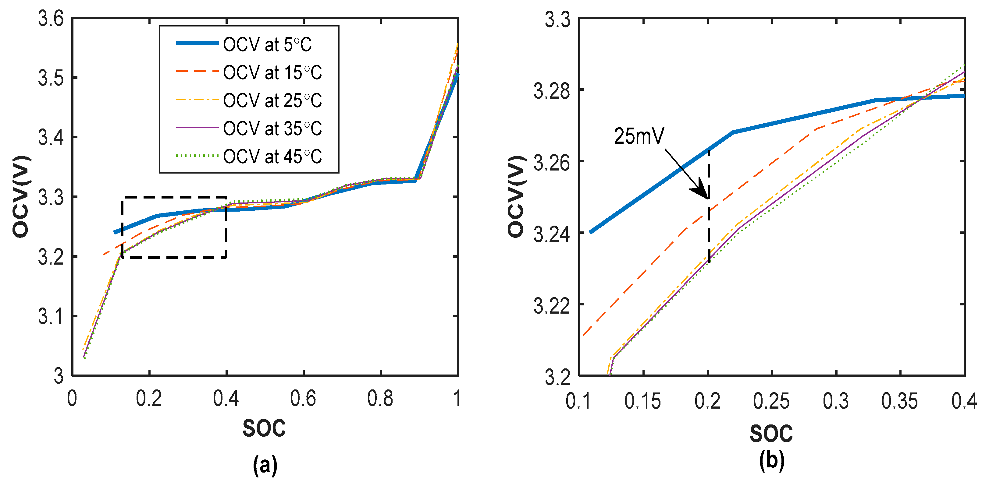
Figure 4.
1-RC equivalent circuit model of a single battery cell in Simscape [67].
Figure 4.
1-RC equivalent circuit model of a single battery cell in Simscape [67].

Figure 5.
Simulation model of single battery cell in Simscape [67].
Figure 5.
Simulation model of single battery cell in Simscape [67].
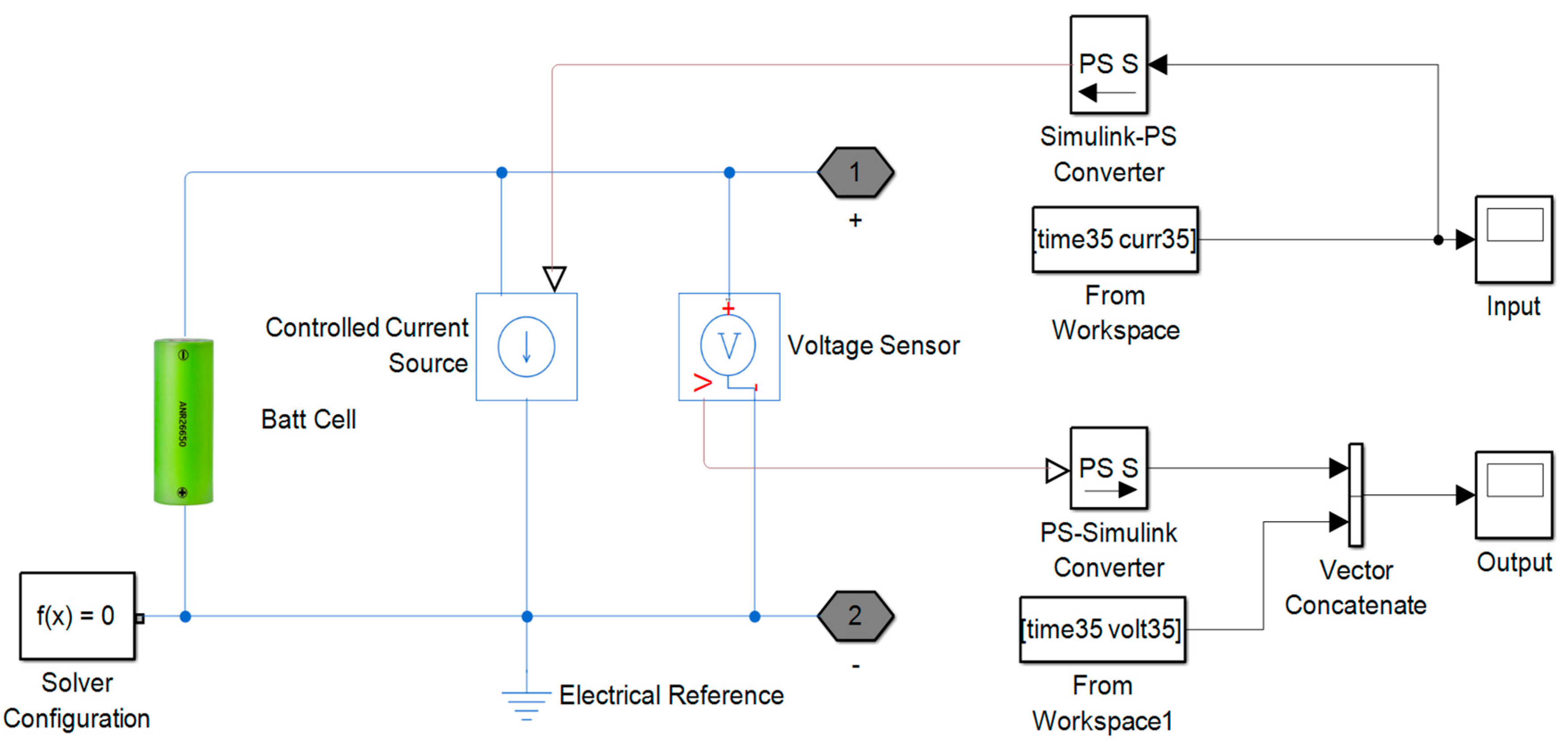
Figure 6.
(a) Cell #1 model validated at 35 °C; (b) corresponding error between simulation and experiment results.
Figure 6.
(a) Cell #1 model validated at 35 °C; (b) corresponding error between simulation and experiment results.
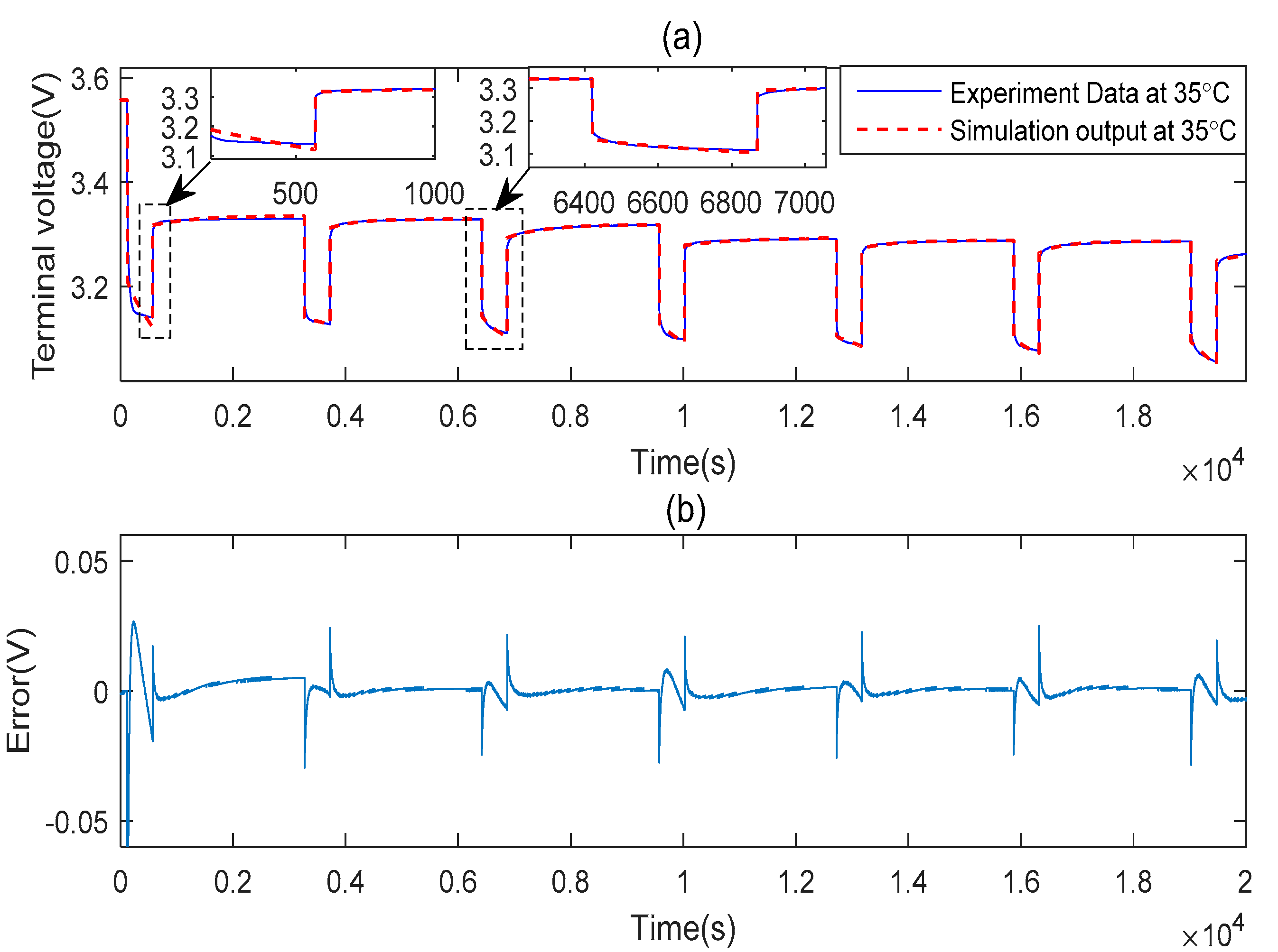
Figure 7.
(a) Actual 12-cell battery prototype with temperature sensor placed at top surface of each cell; (b) simulation model of 12-cell battery in Simscape [67].
Figure 7.
(a) Actual 12-cell battery prototype with temperature sensor placed at top surface of each cell; (b) simulation model of 12-cell battery in Simscape [67].
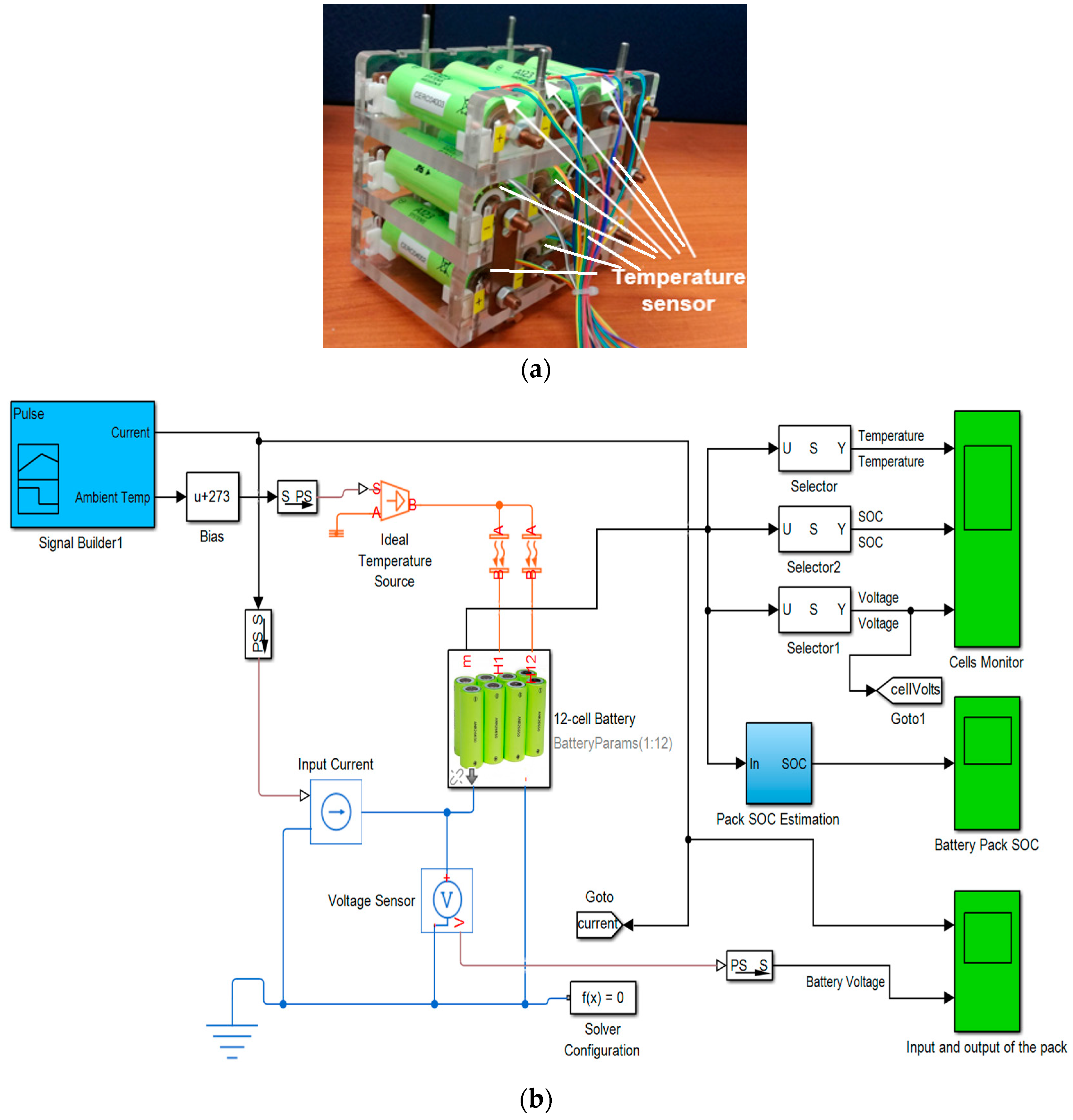
Figure 8.
ELM architecture.

Figure 9.
EKF algorithm flowchart.

Figure 10.
SOC estimation using EKF-based approaches and ELM.

Figure 11.
Different number of neurons used in BP, RBF, and ELM.
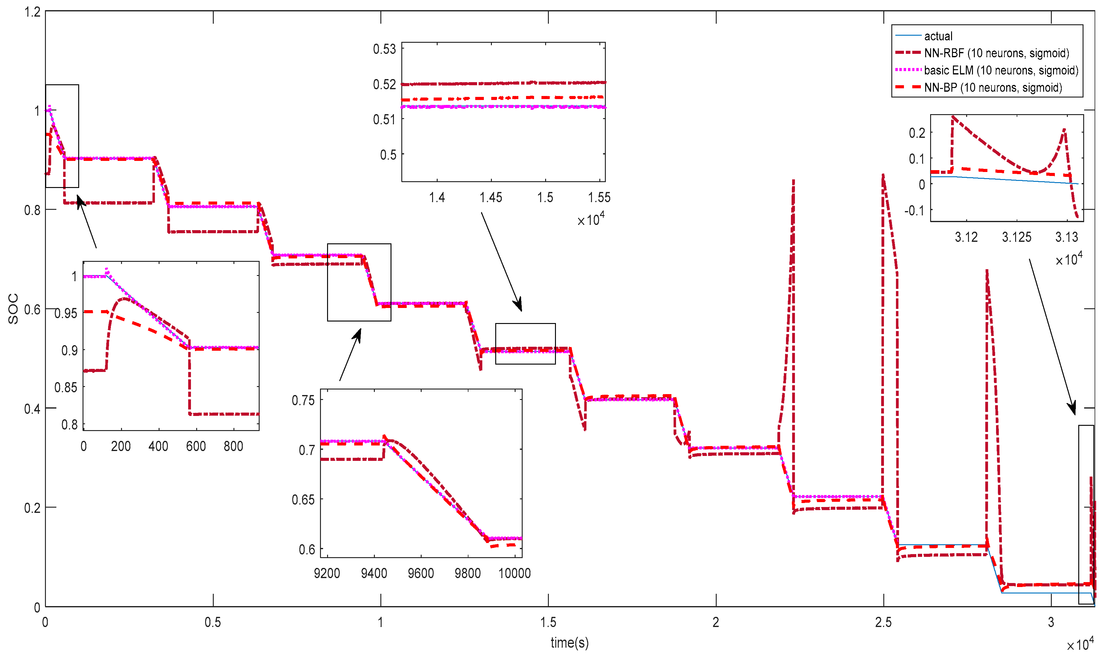
Figure 12.
Different number of neurons used in basic ELM.
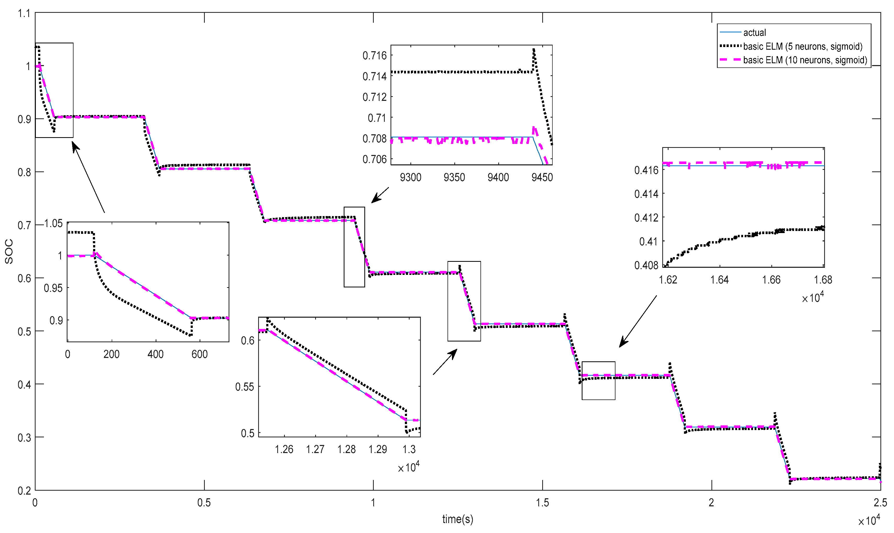
Figure 13.
Different number of neurons used in BP.
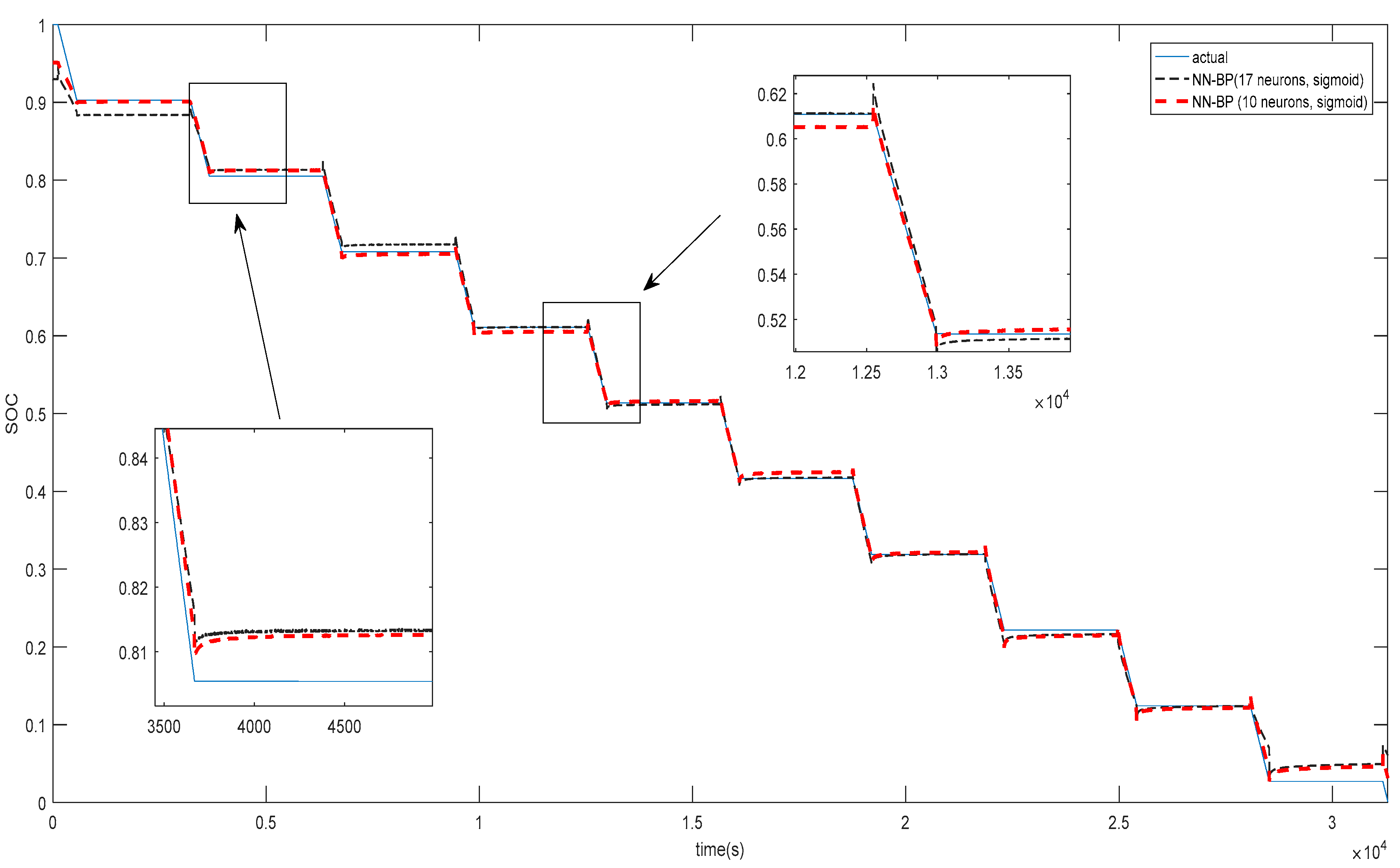
Figure 14.
Different number of neurons in RBF.

Figure 15.
SOC testing performance of online sequential ELM at 25 °C ambient temperature (for different neuron numbers). (a) 5 neurons, (b) 10 neurons, (c) 20 neurons.
Figure 15.
SOC testing performance of online sequential ELM at 25 °C ambient temperature (for different neuron numbers). (a) 5 neurons, (b) 10 neurons, (c) 20 neurons.

Figure 16.
SOC testing performance of adaptive online sequential ELM at 25 °C ambient temperature (for different neuron numbers). (a) 5 neurons, (b) 10 neurons, (c) 20 neurons.
Figure 16.
SOC testing performance of adaptive online sequential ELM at 25 °C ambient temperature (for different neuron numbers). (a) 5 neurons, (b) 10 neurons, (c) 20 neurons.

Figure 17.
SOC standard deviation of adaptive online sequential ELM (five neurons).
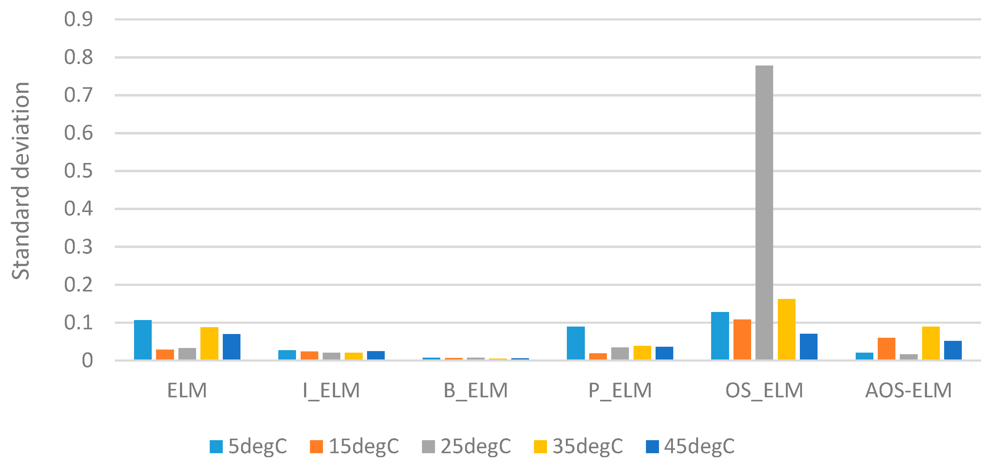
Figure 18.
SOC standard deviation of adaptive online sequential ELM (10 neurons).

Figure 19.
SOC standard deviation of adaptive online sequential ELM (20 neurons).

Figure 20.
Testing RMSE for a 12-cell battery at 25 °C for five neurons (N0 = 200, block range = 847, sinusoidal activation function).
Figure 20.
Testing RMSE for a 12-cell battery at 25 °C for five neurons (N0 = 200, block range = 847, sinusoidal activation function).

Figure 21.
Training time for a 12-cell battery at 25 °C for five neurons (N0 = 200, block range = 847, sinusoidal activation function).
Figure 21.
Training time for a 12-cell battery at 25 °C for five neurons (N0 = 200, block range = 847, sinusoidal activation function).
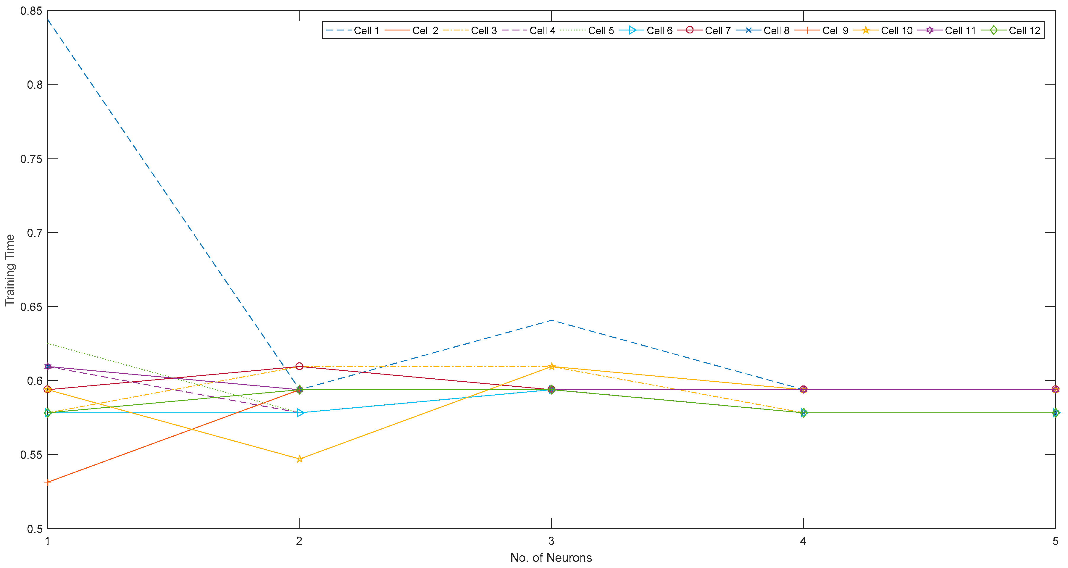
Figure 22.
Training time and testing RMSE for a 12-cell battery at 25 °C for five neurons (N0 = 200, block range = 847, sinusoidal activation function).
Figure 22.
Training time and testing RMSE for a 12-cell battery at 25 °C for five neurons (N0 = 200, block range = 847, sinusoidal activation function).
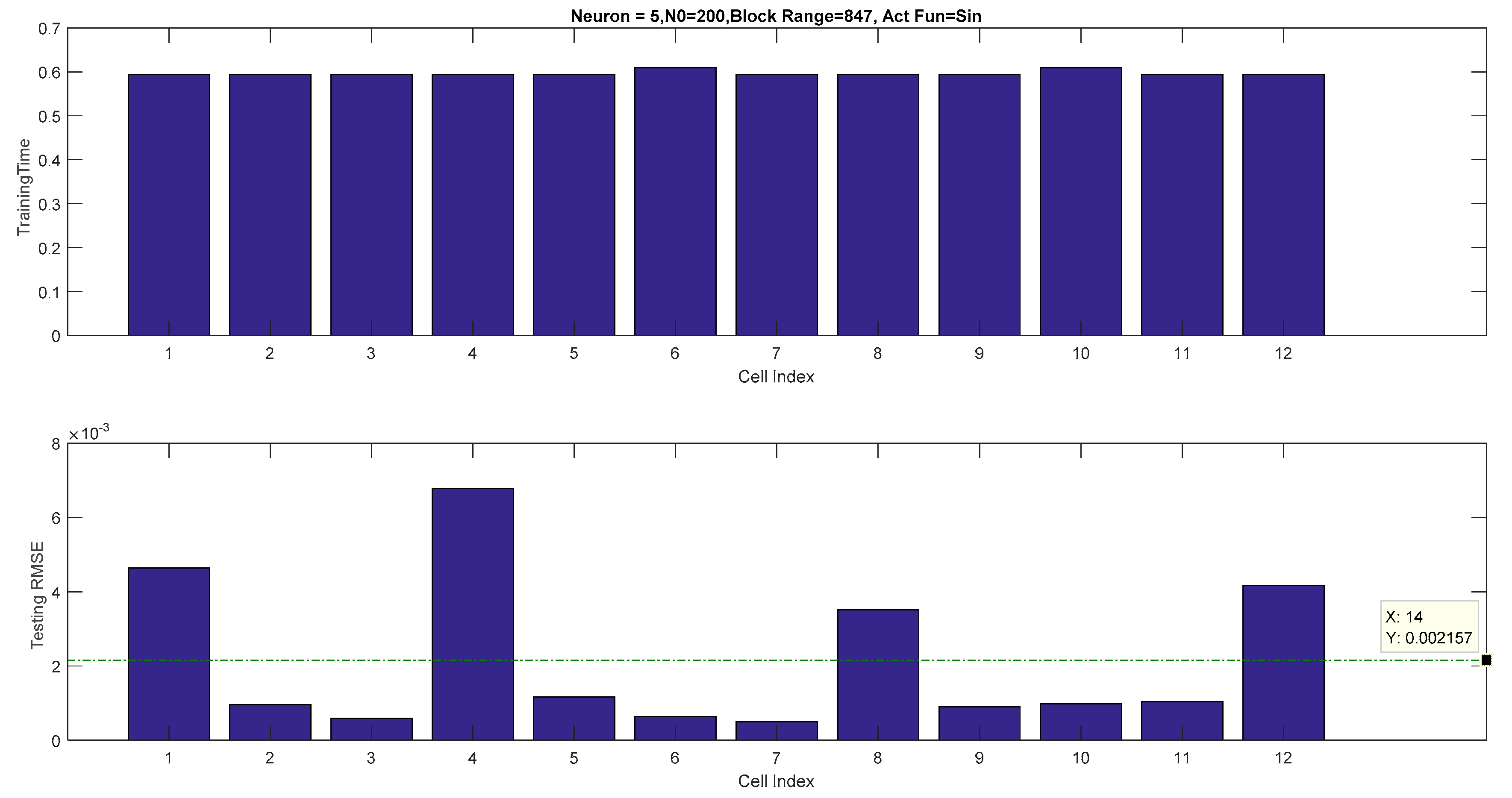
Figure 23.
Pack SOC for a 12-cell battery at 25 °C for five neurons (N0 = 200, block range = 847, sinusoidal activation function).
Figure 23.
Pack SOC for a 12-cell battery at 25 °C for five neurons (N0 = 200, block range = 847, sinusoidal activation function).

Table 1.
Primary specifications of cell (obtained from the a123batteries.com datasheet). CCCV: constant-current-constant-voltage.
Table 1.
Primary specifications of cell (obtained from the a123batteries.com datasheet). CCCV: constant-current-constant-voltage.
| Dimensions (mm) | Ø26 × 65 |
|---|---|
| Mass (g) | 76 |
| Nominal Voltage (V) | 3.3 |
| Cell Capacity (nominal/minimum) (0.5 C Rate) | 2.5/2.4 |
| Recommended Standard Charge Method | 1 C (2.5 A) to 3.6 V CCCV |
| Maximum Continuous Discharge | 50 A |
| Internal Impedance (1 kHz AC typical, mΩ) | 6 |
| Cycle Life at 20 A Discharge, 100% DOD | >1000 cycles |
| Operating Temperature | −30 °C to 55 °C |
| Storage Temperature | −40 °C to 60 °C |
Table 2.
Experimental results of static capacities (Ah) under different ambient temperatures for 12-cell.
Table 2.
Experimental results of static capacities (Ah) under different ambient temperatures for 12-cell.
| Static Capacities (Ah) | 5 °C | 15 °C | 25 °C | 35 °C | 45 °C |
|---|---|---|---|---|---|
| Cell 01 | 2.2369 | 2.4474 | 2.5642 | 2.5693 | 2.5706 |
| Cell 02 | 2.2504 | 2.4972 | 2.5846 | 2.5898 | 2.5922 |
| Cell 03 | 2.2478 | 2.4868 | 2.5788 | 2.5792 | 2.5868 |
| Cell 04 | 2.2560 | 2.4468 | 2.5626 | 2.5685 | 2.5796 |
| Cell 05 | 2.2668 | 2.4724 | 2.5905 | 2.5945 | 2.6265 |
| Cell 06 | 2.2565 | 2.4479 | 2.5635 | 2.5690 | 2.5798 |
| Cell 07 | 2.2429 | 2.4464 | 2.5655 | 2.5668 | 2.5725 |
| Cell 08 | 2.2519 | 2.4985 | 2.5762 | 2.5785 | 2.5935 |
| Cell 09 | 2.2389 | 2.4495 | 2.5662 | 2.5683 | 2.5726 |
| Cell 10 | 2.2468 | 2.4456 | 2.5654 | 2.5682 | 2.5746 |
| Cell 11 | 2.2358 | 2.4462 | 2.5622 | 2.5675 | 2.5698 |
| Cell 12 | 2.2469 | 2.4584 | 2.5742 | 2.5783 | 2.5866 |
Table 3.
Experimental results of Open-circuit voltage (OCV) look-up table for Cell #1 (in V).
| State-Of-Charge (SOC) | 5 °C | 15 °C | 25 °C | 35 °C | 45 °C |
|---|---|---|---|---|---|
| 0.1 | 3.2520 | 3.2208 | 3.1586 | 3.1295 | 3.1218 |
| 0.2 | 3.2620 | 3.2412 | 3.2328 | 3.2308 | 3.2315 |
| 0.3 | 3.2782 | 3.2700 | 3.2625 | 3.2610 | 3.2598 |
| 0.4 | 3.2785 | 3.2820 | 3.2800 | 3.2835 | 3.2840 |
| 0.5 | 3.2820 | 3.2882 | 3.2898 | 3.2910 | 3.2935 |
| 0.6 | 3.2892 | 3.2898 | 3.2905 | 3.2915 | 3.2938 |
| 0.7 | 3.3268 | 3.3278 | 3.3286 | 3.3296 | 3.3295 |
| 0.8 | 3.3285 | 3.3286 | 3.3292 | 3.3298 | 3.3308 |
| 0.9 | 3.3305 | 3.3312 | 3.3324 | 3.3302 | 3.3312 |
| 1 | 3.5125 | 3.5230 | 3.5562 | 3.5406 | 3.5806 |
Table 4.
Experimental results of R0, R1 and C1 look-up table for Cell #1.
| SOC | Parameters | 5 °C | 15 °C | 25 °C | 45 °C |
|---|---|---|---|---|---|
| 0.1 | (Ω) | 0.1110 | 0.1032 | 0.0959 | 0.0658 |
| (Ω) | 0.0356 | 0.0207 | 0.0103 | 0.0125 | |
| (F) | 9893.7 | 61,774 | 76,375 | 1518.4 | |
| 0.2 | (Ω) | 0.1059 | 0.1022 | 0.0931 | 0.0758 |
| (Ω) | 0.0272 | 0.0322 | 0.0246 | 0.0058 | |
| (F) | 11,125 | 13,142 | 16,793 | 22,556 | |
| 0.3 | (Ω) | 0.1111 | 0.1038 | 0.0952 | 0.0808 |
| (Ω) | 0.0187 | 0.0214 | 0.0198 | 0.0137 | |
| (F) | 8920.7 | 33,225 | 35,000 | 52,492 | |
| 0.4 | (Ω) | 0.1111 | 0.1046 | 0.0936 | 0.0779 |
| (Ω) | 0.0249 | 0.0200 | 0.0155 | 0.0108 | |
| (F) | 18,759 | 43,469 | 70,472 | 143,670 | |
| 0.5 | (Ω) | 0.1169 | 0.1049 | 0.0945 | 0.0780 |
| (Ω) | 0.0138 | 0.0238 | 0.0199 | 0.0126 | |
| (F) | 7912.0 | 19,026 | 26,581 | 41,221 | |
| 0.6 | (Ω) | 0.1182 | 0.1067 | 0.0967 | 0.0802 |
| (Ω) | 0.0463 | 0.0262 | 0.0166 | 0.0078 | |
| (F) | 7342.2 | 14,102 | 24,086 | 52,145 | |
| 0.7 | (Ω) | 0.1060 | 0.1155 | 0.1007 | 0.0794 |
| (Ω) | 0.0440 | 0.0312 | 0.0266 | 0.0466 | |
| (F) | 786.56 | 24,213 | 38,256 | 58,391 | |
| 0.8 | (Ω) | 0.0966 | 0.1219 | 0.1060 | 0.0868 |
| (Ω) | 0.0688 | 0.0805 | 0.0488 | 0.0219 | |
| (F) | 1108.1 | 9986.9 | 30,219 | 318,610 | |
| 0.9 | (Ω) | 0.1313 | 0.1366 | 0.1018 | 0.0714 |
| (Ω) | 0.0953 | 0.0838 | 0.0956 | 0.9699 | |
| (F) | 1608.9 | 7012.3 | 9762.6 | 11,217 | |
| 1.0 | (Ω) | 0.2000 | 0.4146 | 0.1378 | 0.0970 |
| (Ω) | 0.2690 | 0.9385 | 0.8782 | 1.0000 | |
| (F) | 1121.8 | 24.292 | 63.287 | 7.6600 |
Table 5.
RMSE between simulation and experiment of terminal voltage in per-unit basis (percentage).
| Cell Index | 5 °C | 15 °C | 25 °C | 45 °C |
|---|---|---|---|---|
| Cell 01 | 0.1554 | 0.1718 | 0.1401 | 0.0879 |
| Cell 02 | 0.5307 | 0.2340 | 0.1924 | 0.1650 |
| Cell 03 | 0.5483 | 0.2344 | 0.1890 | 0.1785 |
| Cell 04 | 0.5307 | 0.2592 | 0.1890 | 0.2141 |
| Cell 05 | 0.5859 | 0.2339 | 0.1943 | 0.2141 |
| Cell 06 | 0.5307 | 0.2478 | 0.1925 | 0.1951 |
| Cell 07 | 0.5483 | 0.2478 | 0.1943 | 0.1650 |
| Cell 08 | 0.6078 | 0.3275 | 0.2033 | 0.1979 |
| Cell 09 | 0.7179 | 0.3715 | 0.2499 | 0.3117 |
| Cell 10 | 0.7900 | 0.3961 | 0.2929 | 0.3732 |
| Cell 11 | 0.8403 | 0.4595 | 0.3599 | 0.4264 |
| Cell 12 | 0.8819 | 0.5463 | 0.4173 | 0.5179 |
Table 6.
RMSE for SOC estimated in different cells.
| Battery Cells | Cell 1 | Cell 2 | Cell 3 | Cell 4 | Cell 5 | Cell 6 |
|---|---|---|---|---|---|---|
| RMSE (10−3) | 6.970 | 7.059 | 7.048 | 7.059 | 7.048 | 7.058 |
| Battery Cells | Cell 7 | Cell 8 | Cell 9 | Cell 10 | Cell 11 | Cell 12 |
| RMSE (10−3) | 7.070 | 7.042 | 7.048 | 7.037 | 7.069 | 7.387 |
Table 7.
Comparing SOC estimation performance using EKF-based approaches and ELM.
| Methods | RMSE | Computation Time (s) |
|---|---|---|
| EKF | 0.0149 | 0.0625 |
| STEKF | 0.0079 | 0.1094 |
| CKF | 0.0066 | 0.0938 |
| SMO | 0.0061 | 7.4844 |
| ELM (10 neurons, sigmoid) | 0.0004 | 0.0313 |
Table 8.
Summary of RMSE and training time for backpropagation (BP), radial basis function (RBF) and basic ELM.
Table 8.
Summary of RMSE and training time for backpropagation (BP), radial basis function (RBF) and basic ELM.
| Methods | RMSE | Training Time (s) |
|---|---|---|
| BP (17 neurons, sigmoid) | 4.8790 | 1952.00 |
| BP (10 neurons, sigmoid) | 2.4540 | 4066.00 |
| RBF (17 neurons, sigmoid, spread = 1, goal = 1 × 10⁻³, df = 1) | 0.0990 | 626.000 |
| RBF (10 neurons, sigmoid) | 0.1000 | 417.600 |
| Basic ELM (5 neurons, sigmoid) | 0.0178 | 0.00001 |
| Basic ELM (10 neurons, sigmoid) | 0.0004 | 0.03100 |
Table 9.
Results of online sequential ELM with radial basis function (Number of initial training data used, N0 = 80; size of block of data learned in each step, Block = 1270).
Table 9.
Results of online sequential ELM with radial basis function (Number of initial training data used, N0 = 80; size of block of data learned in each step, Block = 1270).
| Parameters | # Hidden Nodes = 5 | # Hidden Nodes = 10 | # Hidden Nodes = 20 | |||||||||
|---|---|---|---|---|---|---|---|---|---|---|---|---|
| Training Time | Training RMSE | Testing Time | Testing RMSE | Training Time | Training RMSE | Testing Time | Testing RMSE | Training Time | Training RMSE | Testing Time | Testing RMSE | |
| 5 °C (N0 = 50, Block = 1270) | 3.8594 | 0.1034 | 0 | 0.1171 | 3.7031 | 0.1052 | 0.0313 | 0.1379 | 3.9063 | 0.1356 | 0 | 0.1357 |
| 15 °C (N0 = 60, Block = 1270) | 3.6875 | 0.0646 | 0.0313 | 0.0968 | 3.9531 | 0.1233 | 0 | 0.1703 | 3.7969 | 0.1077 | 0.0313 | 0.1506 |
| 25 °C (N0 = 80, Block = 1270) | 3.6406 | 0.0554 | 0 | 0.0655 | 3.9531 | 0.1306 | 0 | 0.0527 | 3.9688 | 0.0480 | 0 | 0.0527 |
| 35 °C (N0 = 80, Block = 635) | 4.0781 | 0.0369 | 0 | 0.0512 | 2.7813 | 0.0844 | 0.0313 | 0.0970 | 1.4219 | 0.1178 | 0 | 0.1278 |
| 45 °C (N0 = 90, Block = 847) | 4.0625 | 0.1803 | 0 | 0.2010 | 2.8438 | 0.1199 | 0 | 0.1483 | 2.0625 | 0.1637 | 0.0469 | 0.1914 |
| 2-norm | 8.6534 | 0.2276 | 0.0313 | 0.2653 | 7.7968 | 0.2546 | 0.0443 | 0.2867 | 7.1905 | 0.2701 | 0.0564 | 0.3112 |
Table 10.
Results of adaptive online sequential ELM with sinusoidal activation function (Number of initial training data used, N0 and the range of the size of data block randomly generated in each iteration of sequential learning phase, Block_Range are different).
Table 10.
Results of adaptive online sequential ELM with sinusoidal activation function (Number of initial training data used, N0 and the range of the size of data block randomly generated in each iteration of sequential learning phase, Block_Range are different).
| Parameters | # Hidden Nodes = 5 | # Hidden Nodes = 10 | # Hidden Nodes = 20 | |||||||||
|---|---|---|---|---|---|---|---|---|---|---|---|---|
| Training Time | Training RMSE | Testing Time | Testing RMSE | Training Time | Training RMSE | Testing Time | Testing RMSE | Training Time | Training RMSE | Testing Time | Testing RMSE | |
| 5 °C (N0 = 100, Block_Range = 847) | 1.1875 | 0.1222 | 0 | 0.0609 | 0.9844 | 0.0015 | 0.0469 | 0.0020 | 1.3906 | 0.0349 | 0 | 0.0528 (Block_Range = 590) |
| 15 °C (N0 = 200, Block_Range = 1270) | 1.0469 | 0.0037 | 0.0156 | 0.0043 | 0.7500 | 0.0013 | 0 | 0.0011 | 0.7344 | 0.0033 | 0 | 0.0036 (Block_Range = 590) |
| 25 °C (N0 = 200, Block_Range = 1270) | 0.9375 | 0.0148 | 0.0313 | 0.0181 | 0.9844 | 0.0018 | 0 | 0.0021 | 1.1406 | 0.00002 | 0 | 0.00002 (Block_Range = 590) |
| 35 °C (N0 = 340, Block_Range = 1270) | 0.7344 | 0.0153 | 0 | 0.0225 | 1.0156 | 0.0025 | 0 | 0.0021 | 0.9844 | 0.0007 | 0 | 0.0011 (Block_Range = 590) |
| 45 °C (N0 = 590, Block_Range = 1270) | 0.7031 | 0.0464 | 0 | 0.0450 | 0.9844 | 0.0007 | 0 | 0.0011 | 0.7656 | 0.0008 | 0 | 0.0009 (Block_Range = 590) |
| 2-norm | 2.1021 | 0.1325 | 0.0350 | 0.0812 | 2.1216 | 0.0037 | 0.0469 | 0.0039 | 2.3085 | 0.0351 | 0 | 0.0529 |
Table 11.
Results of adaptive online sequential ELM with sinusoidal activation function using five neurons.
Table 11.
Results of adaptive online sequential ELM with sinusoidal activation function using five neurons.
| Number of Initial Training Data Used (N0) | Range of the Size of Data Block Randomly Generated in Each Iteration of Sequential Learning Phase (Block Range) | Testing RMSE |
|---|---|---|
| 80 | 847 | 0.0324 |
| 100 | 0.0083 | |
| 200 | 0.0043 | |
| 80 | 2540 | 20.631 |
| 1270 | 6.5865 | |
| 847 | 0.2373 |
© 2018 by the authors. Licensee MDPI, Basel, Switzerland. This article is an open access article distributed under the terms and conditions of the Creative Commons Attribution (CC BY) license (http://creativecommons.org/licenses/by/4.0/).
Share and Cite
MDPI and ACS Style
Chin, C.S.; Gao, Z. State-of-Charge Estimation of Battery Pack under Varying Ambient Temperature Using an Adaptive Sequential Extreme Learning Machine. Energies 2018, 11, 711. https://doi.org/10.3390/en11040711
AMA Style
Chin CS, Gao Z. State-of-Charge Estimation of Battery Pack under Varying Ambient Temperature Using an Adaptive Sequential Extreme Learning Machine. Energies. 2018; 11(4):711. https://doi.org/10.3390/en11040711
Chicago/Turabian StyleChin, Cheng Siong, and Zuchang Gao. 2018. "State-of-Charge Estimation of Battery Pack under Varying Ambient Temperature Using an Adaptive Sequential Extreme Learning Machine" Energies 11, no. 4: 711. https://doi.org/10.3390/en11040711
Note that from the first issue of 2016, this journal uses article numbers instead of page numbers. See further details here.