Identifying Health Status of Wind Turbines by Using Self Organizing Maps and Interpretation-Oriented Post-Processing Tools

Abstract

Background: Identifying the health status of wind turbines becomes critical to reduce the impact of failures on generation costs (between 25–35%). This is a time-consuming task since a human expert has to explore turbines individually. Methods: To optimize this process, we present a strategy based on Self Organizing Maps, clustering and a further grouping of turbines based on the centroids of their SOM clusters, generating groups of turbines that have similar behavior for subsystem failure. The human expert can diagnose the wind farm health by the analysis of a small each group sample. By introducing post-processing tools like Class panel graphs and Traffic lights panels, the conceptualization of the clusters is enhanced, providing additional information of what kind of real scenarios the clusters point out contributing to a better diagnosis. Results: The proposed approach has been tested in real wind farms with different characteristics (number of wind turbines, manufacturers, power, type of sensors, ...) and compared with classical clustering. Conclusions: Experimental results show that the states healthy, unhealthy and intermediate have been detected. Besides, the operational modes identified for each wind turbine overcome those obtained with classical clustering techniques capturing the intrinsic stationarity of the data.

1. Introduction

Wind energy, the most growing renewable source [1], helps to meet the demanding climate and energy targets for 2020 set by the EU Commission [2]. Together with these targets, it was established that at least 20% of electricity production must come from sustainable sources [3], among which wind farms are. Wind farms operation and maintenance costs (O&M) represents from 10% to 35% of the overall generation costs [4]. Reducing this amount, the wind farms will be more competitive concerning fossil fuels and accelerate this transition [5].

In the management of wind farms, turbines are scheduled to be maintained every 2500 to 5000 h with preventive maintenance. However, the preventive maintenance operation frequency is insufficient to detect and predict device status and anticipate potential failures. Unexpected stop of turbines has significant costs since they often are placed far from urban areas and several days may be required to wait for the necessary new component and make in situ reparations. To get an idea, about 15% of total turbine cost [6] raises every time that a gearbox needs to be replaced unexpectedly, this representing about a 25% of the total downtime [7].

Getting accurate information about potential failures requires continuous monitoring and diagnosis of turbines health status, and the development of preventive maintenance strategies, which avoid unexpected failures of wind turbines. Expert knowledge plays a fundamental role in diagnosing turbines. However, exhaustive analysis of the whole set of wind turbines of a given wind farm cannot be made by a human expert. When a wind farm starts being monitored, and mainly if it contains a large number of turbines, the first big challenge is to identify a reduced set of representative turbines for detailed inspection. These require, as a first stage, grouping the turbines according to the status of each of their primary subsystems.

Modern wind turbines record more than 200 analog variables [8] at intervals of 5 to 10 min using their SCADA (Supervisory Control and Data Acquisition) system. The SCADA system provides information about temperatures, electrical indicators, physical positions, speeds, vibration, etc. [9]. The analogic variables are the continuous readings from the different wind turbine’s sensors along the time; the SCADA also provides discrete variables which are generated by failure events. Through SCADA-based condition monitoring, detailed data is provided, and this data is suitable to be exploited to find the different wind turbines operation regimes that allow grouping by turbines of similar health status. The exhaustive handmade exploration of turbine variables becomes an unfeasible task. There are many manufacturers, and there is no standardization on how event data is reported. This means that the different variables names and also were they are physically is different from manufacturer to manufacturer. The failure events are also heterogeneous in format and meaning not having a generic code to reference a specific type of physical failure like a gearbox breakdown. Because of this significant amount of data has to be checked, and the number of different working conditions is high, this is why the attention of human experts can only focus on a few turbines, and why groups of turbines associated with similar health status need to be identified. SCADA data is a rich source of information. Taking advantage of a proper analysis of these data, automatic monitoring systems, and decision support tools can be developed, thus contributing to the better planning of maintenance operations and, as a consequence, to decrease operating costs. Data Science and machine learning techniques offer appropriate methods and approach to tackle this tasks.

The purpose of this work is to propose a new methodology based on data science and automatic interpretation techniques to identify a reduced set of wind turbines, representative enough of a complete wind farm, to be carefully inspected by human experts in a reasonable time, by providing support to decision-making about preventive maintenance of the park. The significance of the work is high, as exhaustive inspection of all wind turbines in the farm is no affordable, and the economic impact of reducing unexpected failures is considerable. The primary hypothesis of this work is that the proposed methodology allows identification of distinct turbine operation regimes, by grouping the turbines of a park accordingly, in such a way that bad health regimes appear in separate groups. These groups should be understood in terms of certain indicators that will support the expert decision to schedule a maintenance operation and, as a consequence the number of unexpected failures is expected to be reduced, overcoming the current state of the art.

This study focuses on a particular type of failure, for simplicity, but the proposed methodology is general. Thus, in this work, the identification of distinct groups of turbines according to the status of the gearbox is pursued, because this is an expensive wind turbine subsystem, with frequent breakdowns that are challenging to repair and is the responsible for expensive maintenance costs due to its components, as explained before.

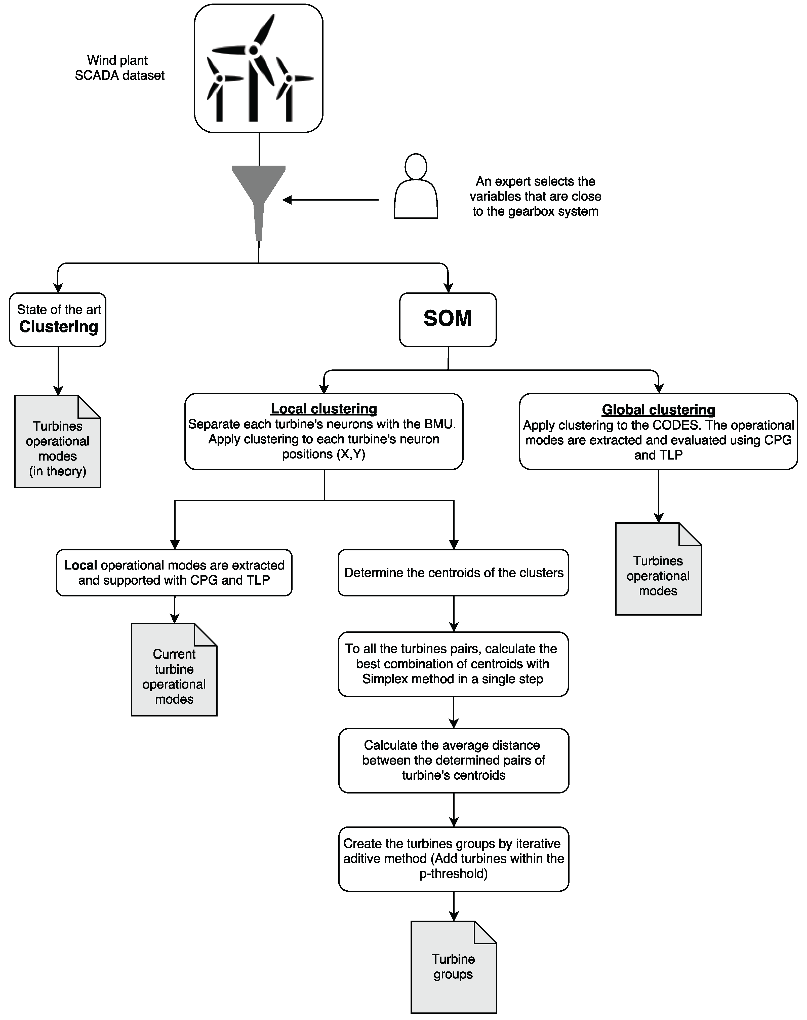
Several strategies exist for implementing Condition Monitoring Systems (CMS). One of the most popular methods comes from the machine learning field, which is based on Artificial Neural Networks (ANN), is the Self Organizing Maps (SOM) [10]. SOM runs as an unsupervised system and is envisaged as a promising tool due to its sensitivity to detect abnormal operation registers. Therefore, an ANN approach based on SOM can provide a clustering that reflects the nature of the entire set of turbines and significantly reduces the human factor in the consistency criterion. Discovering turbines whose characteristics deviate from normal behavior is useful for experts, who can then focus their attention on them. At the same time, finding turbines in better and more stable conditions allows to take them as a reference in trend systems.

However, as happens with the other ANN systems, the simple use of SOM have some limitations concerning capturing a particular type of complex stationarities and providing a good understanding of the nature of proposed clusters to the experts. Few works have been done on complementing the results provided by SOM with additional tools that bridge the gap between raw data mining results and decision-making processes. In this paper, a data-driven process is proposed with the objective of close this gap. The process combines the clusters discovery using SOM with some further elaboration of the proposed clusters and additional interpretation. The further interpretation is made with oriented tools like Class panel graphs (CPG) [11] or Traffic Lights panels (TLP) [12], both introduced in Section 3, with the objective of identifying a reduced set of turbines to be inspected in situ, using the available SCADA measurements monitoring.

The structure of the paper is the following: Section 2 provides results of the application of the proposed approach to real data, while they have discussed in Section 3 pointing also to future work. Finally, in Section 4 the methodological approach and the context of the resented research in a real wind farm is described.

2. Results

2.1. SOM Dimensions for the Experiments

In this work, data coming from the SCADA system of several wind farms are considered (see Section 4 for details on data used). For conduct the experiments for the wind farm ’Wf1’ (see Table 7), the first step is to decide the size of the SOM. Having R = 17.536 registers (16 turbines × 3 years × 365.3 days), and according to the rule $n=\lceil 5\sqrt{R}\rceil$ [13], the number of units (neurons) to be used should be 663, which represents a SOM of size 25 × 25, approximately. However, as explained in Section 4.4, we will use Topographic error (TE), and the Quantization error (QE) metrics to set the optimal size. Therefore, SOM maps of different sizes have been generated with the data from wind farm ’Wf1’. 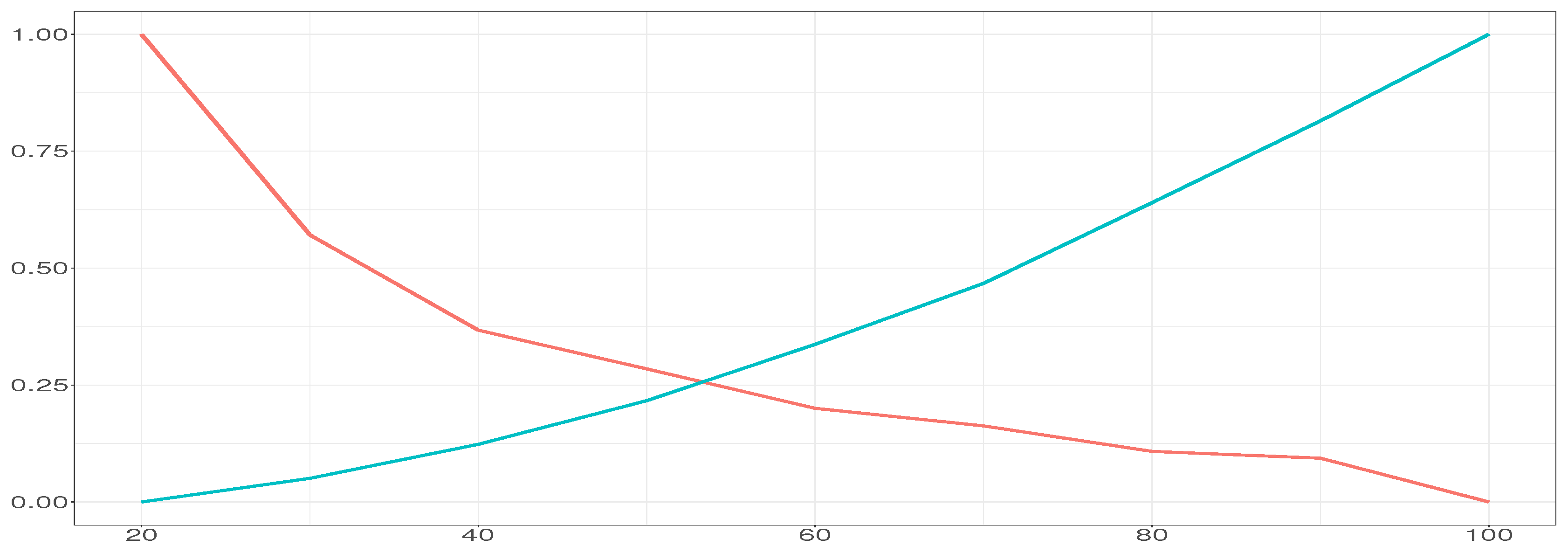The (normalized) evolution of both metrics TE and QE is plotted in Figure 1, for sizes ranging from 20 × 20 (400 neurons) to 100 × 100 (10,000 neurons). We observe how TE drops exponentially when the number of neurons increases, while QE increases with it. The crossing point of both curves is 52, which will be used as the optimal SOM size.

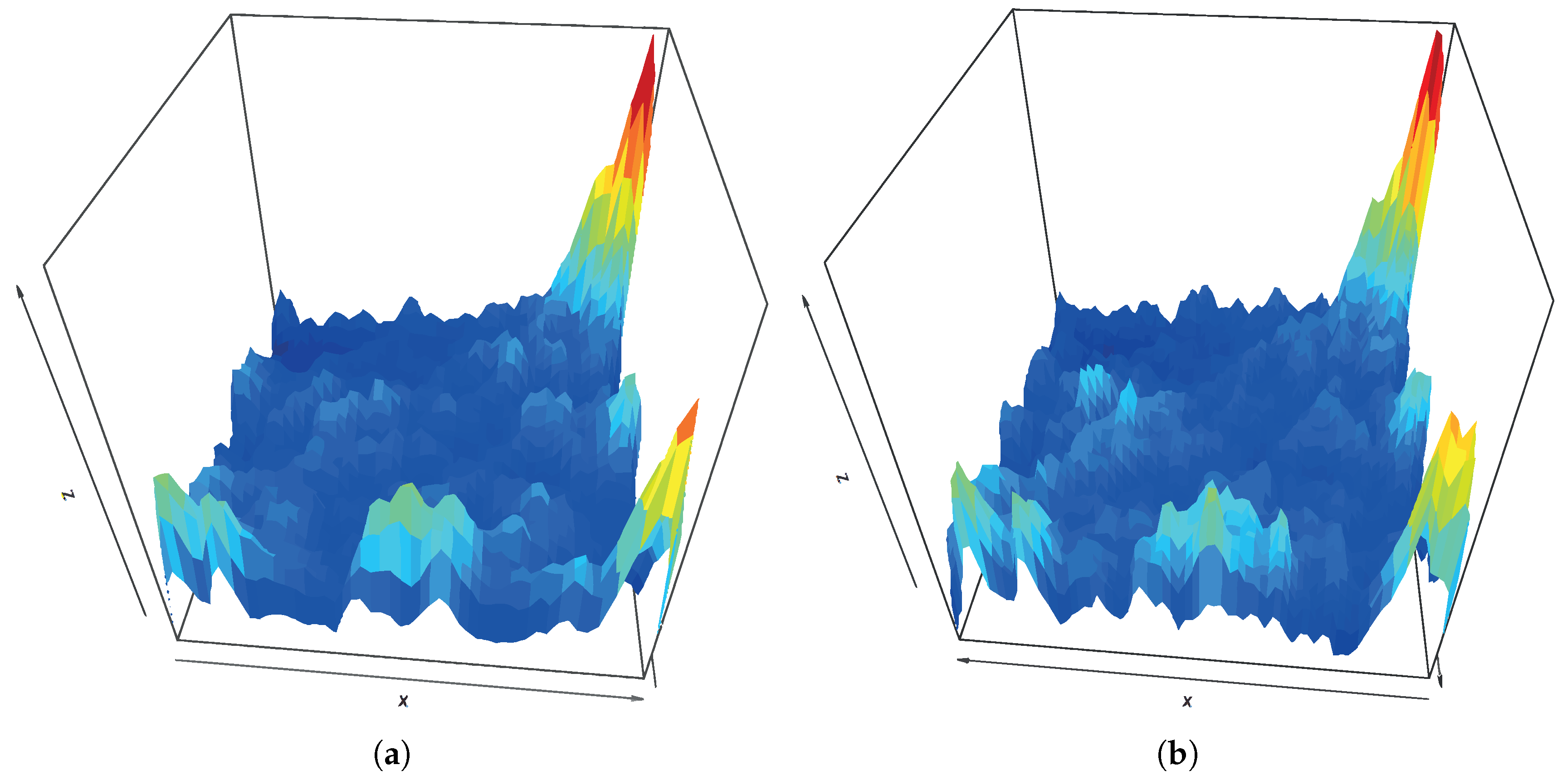
To verify the adequacy of the SOM dimensions, we compared results obtained with a SOM generated, for wind farm ’Wf1’, using the optimal (52 × 52) size and a sub-optimal one (70 × 70). Figure 2a,b represent the U-matrix for sizes 52 × 52 and 70 × 70, respectively. Although they are not equal, the peaks of both maps are located in the same areas and show similar values, indicating that both U-matrix identify the same kind of structure despite being independently created from a different number of neurons.

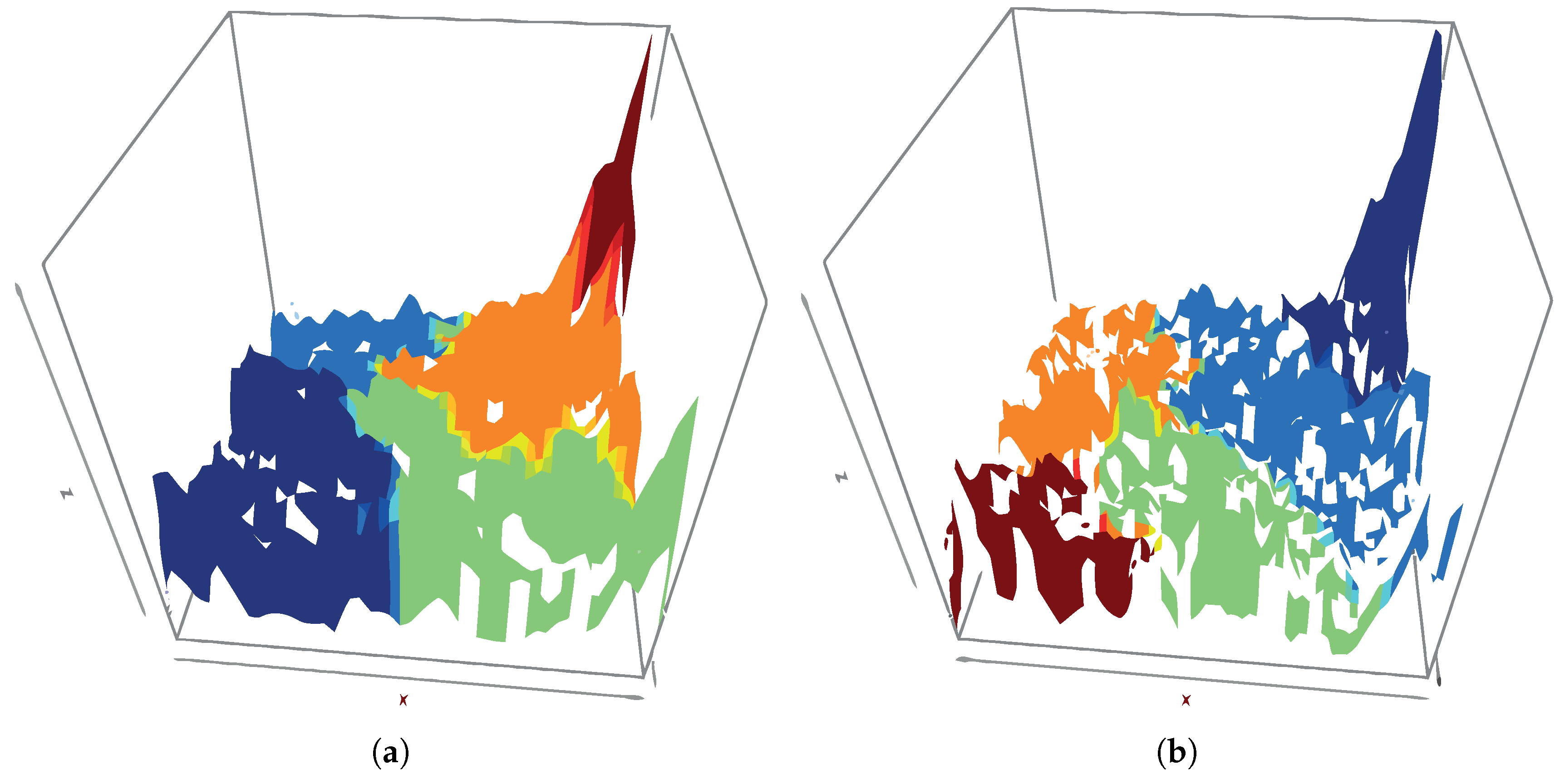
Figure 3a,b show clustering performed on the SOM codes (neuron weights) using the Hierarchical clustering technique for a fixed number of 5 clusters, for 52 × 52 and 70 × 70 maps, respectively. In this figure, the clustering result is plotted over the corresponding U-matrix for each case, to ease the interpretation of the clustering.

In both cases, the clusters in the upper right and lower left map corners appear. These Sections can also be seen in the U-Matrices and show areas with high distance values. Provided that computational costs of SOM increase with the number of neurons and that the impact of increasing the neurons on the identified structures is low, we will use 52 × 52 size.

2.2. Understanding the Results of SOM Clustering

The clustering performed over the SOM codes contains information about the wind turbines. The TLP of the resulting clustering is shown in

Table 1. Traffic Lights Panel of the SOM codes clustering result. The Cluster column indicates the clusters found in Section 2.1.

(see details and meaning of colors in Section 4.7); the corresponding class panel graph with super-imposed TLP is in

Table 2. Class Panel Graph of the SOM codes clustering result vs input variables with TLP super-imposed.

Cluster	Nc	X (1-52)	Y (1-52)	Date-Time (2014-16)	WindSpd (0-16.5) m/s	RotorSpd (0-14) RPM	AmbientTemp (-10-36) °C	Power (-50-3048) KW	GearboxOilTemp-Temp (3-62) °C	GearboxBearing (4-81) °C	PowerWindRatio (-23-242)
C1	4909
C4	4969
C3	5157
C2	1936
C5	524

. Both are performed to support the conceptualization process of the clusters.

Looking into details of each one of the clusters in Figure 3a we identified the following (listed from most general to most particular) cases:

Cluster 1-High-performance regime due to strong wind

(bottom left corner in Figure 3a): This scenario can take place all along the year on windy days, and therefore a variety of ambient temperatures are registered. Its main characteristic is the presence of higher wind. Thus the rotor is in full movement, the wind production is high, the oil temperature is high and so is the temperature of the bearing. The best performance of all the groups.

Cluster 4-Low-performance low wind regime

(top right area in Figure 3a): In this scenario, there is low wind; rotor does not rotate at maximum speed and the power generated is small. Except Cluster 5, this is the weakest generation case, and it can happen all along the year, so air temperatures range widely while bearing and oil temperatures are not very high. Low performance.

Cluster 3-Moderate performance regime in summer due to moderate wind

(bottom right in Figure 3a): Due to an intermediate wind level, the rotor is rotating adequately but not at high speed, so the energy production is low. It is summer time, with high air temperatures, and the oil is warmer than in Cluster 2, but the bearing has its same temperature. Intermediate performance.

Cluster 2-A regime of moderate performance in winter by moderate wind

(top left in Figure 3a): Moderate wind; rotor rotating adequately but not at high speed. It is winter time and therefore the air temperature is cold, the energy production is low, the oil temperature is colder than in Cluster 3 while the bearing temperature is moderate. Intermediate performance. The difference between Cluster 3 and Cluster 2 is the ambient temperature: in both cases, similar wind forces, rotor speed, rotor and bearing temperatures, power and similar performances associated with warmer oil in C3.

Cluster 5-Turbine regimen stopped due to lack of wind on winter days

(supper top right in Figure 3a): A particular scenario in which there is no wind; therefore the rotor is stopped. It occurs cyclically in winter and cold days (low ambient temperature). The power production is sometimes negative, meaning that there is no production but consumption which can be the consequence of the oil heater system or when the wind turbine enters in a start-up phase. Bearing temperature is the lowest among all the clusters. As the oil is heated, the bearing temperature is also heated. The turbines are stopped because there is no wind at all. Zero or negative performance.

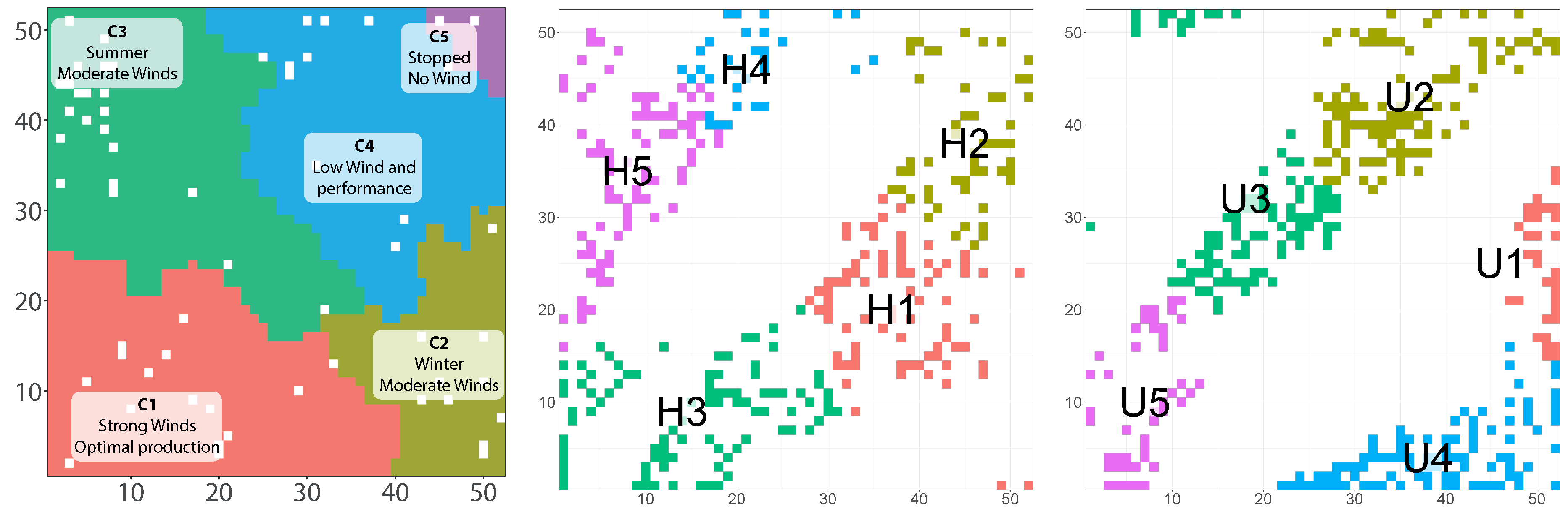
With the use of CPG and TLP a clear interpretation of SOM areas is now obtained. Since the CPG also contains the coordinates of the SOM neurons involved in each class, Figure 4 shows the interpretation of the SOM map.

As mentioned in Section 4.5, different turbines activate different areas of the SOM map. In Figure 4 (middle and right) two different turbines show different patterns or active neurons. In fact, the plot in the middle corresponds to a healthy turbine (H) and the plot in the right to an unhealthy turbine (U). Here we see that some neurons of cluster 2 of the turbine H are the single ones intersecting with the low-performance behavior due to low wind (sector C4 in Figure 4, left), whereas for the turbine U the whole cluster 2 is practically concentrated over regions of low performance or stopped turbine. Also, other topological differences are observed between the two maps. Even if these analyses are accessible by an expert, an automatic procedure to evaluate if this SOM sub-maps are similar or not is required.

2.3. Discrimination of Wind Turbines According to the Neuron Activation in SOM Maps

A local analysis of each turbine is performed by following the methodology presented in Section 4.6. To illustrate the feasibility of the method, the activation of neurons in the SOM maps of two preselected turbines of the same model and wind farm is compared. Turbine H (Figure 4) is in excellent conditions, and we know it has had very few failures. In contrast, turbine U (in Figure 4) had many shortcomings and suffered repairs, among which we highlight a breakdown in the gearbox, which is the system we are analyzing. The results can be seen for a 52 × 52 map in Figure 4, showing how the maps exhibit a near complementary assignation of BMUs. This is the key point to identify turbines with a similar state of health. If we manage to separate the turbines according to how the BMU activations resemble among them, we will be able to group turbines according to their state, and this will make possible to discriminate the unhealthy turbines from the healthy ones. To simplify the comparison between turbines and to have a non-subjective measure, clustering is applied to each wind turbine, and the cluster centroids are calculated. As we will detail in the next sub-Section, these centroids will be later used to group turbines of similar health status.

2.4. Understanding Results of BMU Clustering

For the new local clusters of each turbine, CPGs and TLPs are also developed (see

Table 3. Class panel graphs for turbines H and U with Traffic Lights Panel super-imposed.

Turbine	Local Cluster	Nc	X (1-52)	Y (1-52)	Date-Time (2014-16)	WindSpd (0-16) m/s	RotorSpd (0-14) RPM	AmbientTemp (-9-32) °C	Power (-50-3000) KW	GearboxOilTemp-Temp (10-59) °C	GearboxBearing (10-78) °C	PowerWindRatio (-19-250)
H	H3	334
	H5	252
	H4	105
	H1	237
	H2	166
U	U3	133
	U5	320
	U4	184
	U1	195
	U2	258

). The resulting local patterns shown in each turbine are analyzed.

The post-processing performed with CPGs and TLPs elicits a relationship between clusters local to a wind turbine (built over the BMUs) and global clusters (built over the SOM codes). The operating points do not disappear when analyzing wind turbines separately but might take slightly different behaviors in each local cluster. In the following lines we interpret the relationship between the CPG in Table 2 (prefix C for the general clusters) and the two turbines (H and U) with their local clusters with prefix H for Healthy for the turbine with identifier 119 and U for Unhealthy for the turbine with identifier 133.

Looking first at the similarities of the clusters found with the general CPG, the local clusters U4 and H3 are representing the same operational regime as C1: optimal performance. Also, we observe that local clusters U1 and H1 are pointing to the same pattern as C2: winter, moderate wind. Clusters U5 and H5 are reflected in C3: summer and soft wind. Finally, cluster H1 and U1 can be seen in cluster C2: winter, moderate wind, even if H1 has the variable AmbientTemp slightly higher.

However, we observe that H4 and U3 are similar to C3: summer, soft wind, although each one with a different characteristic, H4 shows AmbientTemp slightly higher and WindSpd slightly lower than C3, however, U3 has AmbientTemp slightly lower. So they could be placed between C3 and C4.

This means that local analysis might elicit specific behaviors or operating conditions of particular turbines and provides more detailed information about the wind farms.

Going further, centroids of all the N clusters of each turbine can be compared together to built a distance matrix between turbines that allows a further turbine regrouping based on considering two turbines similar when they show similar clustering results, i.e., similar sets of N clusters each. As computing the distance between two turbines indeed involving the comparison of two sets of N centroids, the simplex algorithm has been used for this purpose.

2.5. Generating Groups of Turbines Using the Average Distance Between Centroids

As commented on previously, pairwise comparisons of turbines are performed using the distance between their centroids. A global distance for each pair of turbines (calculated as indicated in Section 4.6) is presented in

Table 4. Average distances between the different turbine pairs, calculated as indicated in Section 4.7.

	119	120	121	122	123	124	125	126	127	128	129	130	131	132	133	134
119		5.4	4.7	9.8	3.0	7.1	14.0	11.3	8.4	12.0	7.2	10.7	9.0	9.1	8.4	7.7
120	5.4		7.2	8.7	4.7	4.7	13.5	10.8	10.0	10.9	8.3	11.8	6.8	7.0	9.7	9.6
121	4.7	7.2		9.2	2.7	9.9	12.9	7.8	6.4	10.9	6.9	7.9	8.4	8.6	10.4	6.2
122	9.8	8.7	9.2		9.7	10	5.8	4.5	5.4	7.4	8.3	9.2	8.7	5.5	5.0	8.6
123	3.0	4.7	2.7	9.7		7.9	13.9	9.5	6.5	12.9	6.5	9.3	8.1	8.9	9.5	6.9
124	7.1	4.7	9.9	10.0	7.9		13.7	12.4	12.5	10.9	9.3	12.4	9.2	9.4	10.5	10.5
125	14.0	13.5	12.9	5.8	13.9	13.7		8.1	8.4	9.6	11.7	10.8	11.4	10.1	7.2	12.8
126	11.3	10.8	7.8	4.5	9.5	12.4	8.1		6.3	7.0	8.4	7.3	8.5	6.7	6.5	7.5
127	8.4	10.0	6.4	5.3	6.5	12.5	8.4	6.3		9.2	9.4	8.2	12.9	9.5	6.1	9.8
128	12.0	10.9	10.9	7.4	12.9	10.9	9.6	7.0	9.2		12.1	10.6	7.4	5.1	8.0	11.9
129	7.2	8.3	6.9	8.3	6.5	9.3	11.7	8.4	9.4	12.1		6.6	7.2	9.1	8.0	4.0
130	10.7	11.8	7.9	9.2	9.2	12.4	10.8	7.3	8.2	10.6	6.6		10.0	12.4	9.6	5.2
131	9.0	6.8	8.4	8.7	8.1	9.2	11.4	8.5	12.9	7.4	7.2	10.0		4.8	11.0	8.7
132	9.1	7.0	8.6	5.5	8.9	9.4	10.1	6.7	9.5	5.1	9.1	12.4	4.8		8.3	9.6
133	8.4	9.7	10.4	5.0	9.5	10.5	7.2	6.5	6.1	8.0	8.0	9.6	11.0	8.3		10.0
134	7.7	9.6	6.2	8.6	6.9	10.5	12.8	7.5	9.8	11.9	4.0	5.2	8.7	9.6	10.0

.

Turbines are now regrouped according to their distances and using the algorithm presented in Section 4.6. In this work, the p-threshold is optimized to generate between 3 to 5 groups, because it is a range of clusters that the experts can manage well (as they expect to identify between 3 to 5 prototypical turbines to visit for in situ inspection).

The

Table 5. Results for different p-threshold for wind farm ’Wf1’, together with the expert-based probability of failure and the number of maintenance events generated by each group.

Number of Groups	Group Id	Turbine Identifiers	Expert Probability			Maintenance Events
			Mean	Median	sdv	Count	Mean	Median	sdv
3	1	119, 120, 121, 123, 127, 129, 134	0.282	0.176	0.197	166	23.714	24	6.047
	2	122, 125, 126, 128, 130, 131, 132, 133	0.452	0.394	0.219	191	23.875	22	8.855
	3	124	0.332	0.332	NA	35	35	35	NA
4	1	119, 121, 123, 127, 134	0.254	0.176	0.186	123	24.6	27	6.95
	2	122, 125, 126, 128, 129, 132, 133	0.49	0.554	0.232	176	25.143	23	8.802
	3	120, 124, 131	0.29	0.332	0.124	77	25.667	24	8.622
	4	130	0.356	0.356	NA	16	16	16	NA
5	1	119, 121, 123	0.151	0.172	0.04	68	22.667	19	9.074
	2	129, 130, 134	0.383	0.356	0.159	63	21	19	6.245
	3	122, 125, 126, 127, 132, 133	0.471	0.488	0.248	143	23.833	25	5.811
	4	120, 124, 131	0.29	0.332	0.124	77	25.667	24	8.622
	5	128	0.621	0.621	NA	41	41	41	NA

contains the results of grouping turbines into 3, 4 and 5 groups (column Number of groups) . The group is shown in the Group Id column. Column Turbine identifiers indicates the turbine label. Columns within Expert probability indicate the probability of failure estimated by an expert for the system under evaluation during in situ inspections. Columns within Maintenance events indicates the number of interventions to repair the system under analysis (gearbox).

Since historical wind farm data is available and all events have been collected, the status of the wind turbines at each timestamp is known and can be used as a ground-truth for the evaluation of the discovered clusterings. The turbines that the specialist reported as the worse ones are the 125, 126, 128, 130, 131 and 133. In particular, the wind turbine 133 had broken the gearbox system and the wind turbine 128 had the gearbox changed before it broke. On the contrary, the turbines that we know that are the best ones are the 119 and 121. When analyzing the number of repairs, we see that regardless of the number of groups (3, 4 or 5), the group that had the more repairs always contains most of the damaged turbines, while the group that had fewer repairs contains most of the healthy turbines.

2.6. Comparison with Alternative Clustering Methods

Although that the use of SOM and further clustering over the SOM codes is the current state of the art in wind farm data-driven analysis. An elaborated proposal based on local analysis by wind turbine followed by a global regrouping of similar clusters is presented, this Section is devoted to comparing the achieved results with a much more classic approach that finds clusters avoiding intermediate SOM construction.

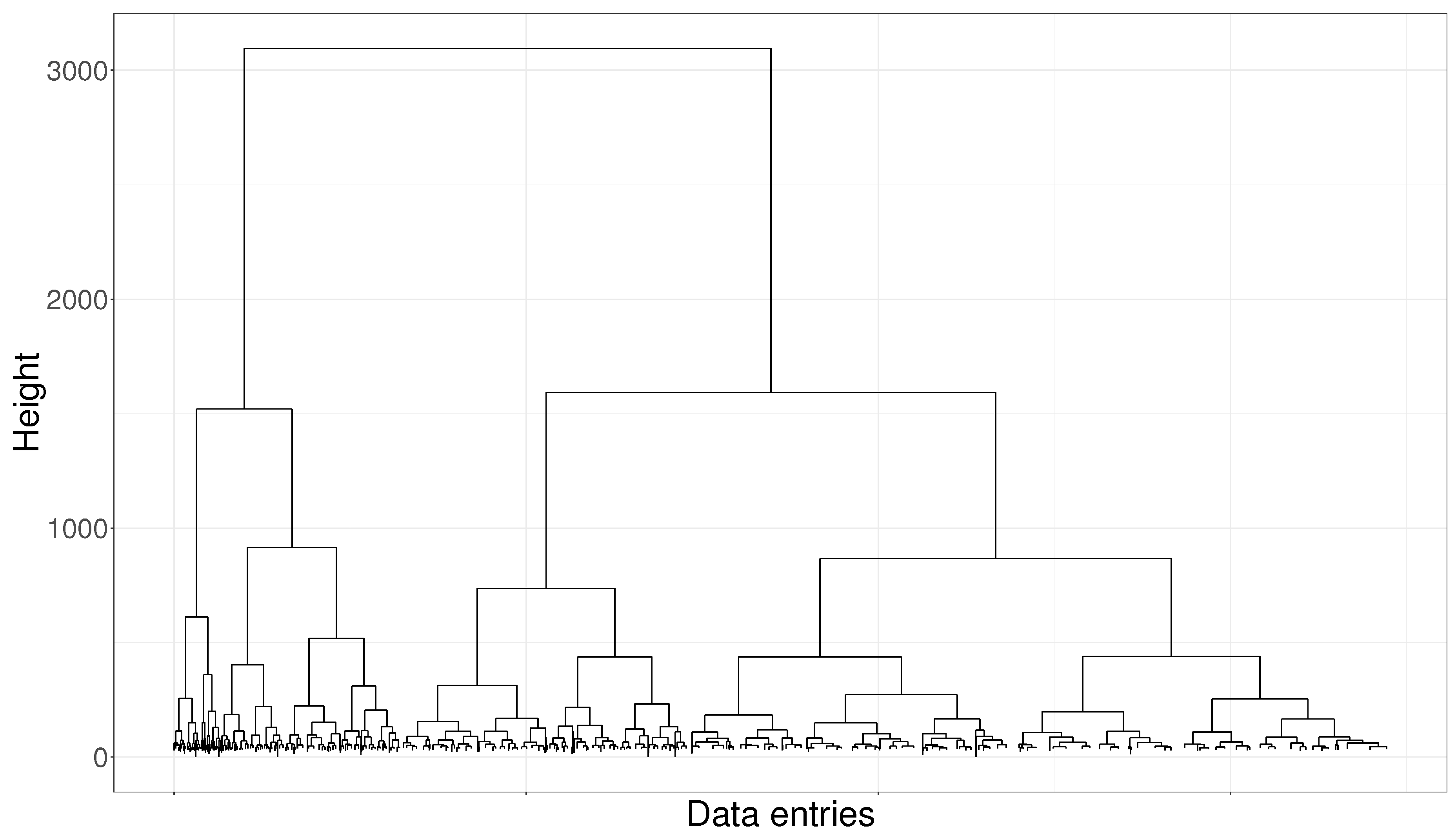
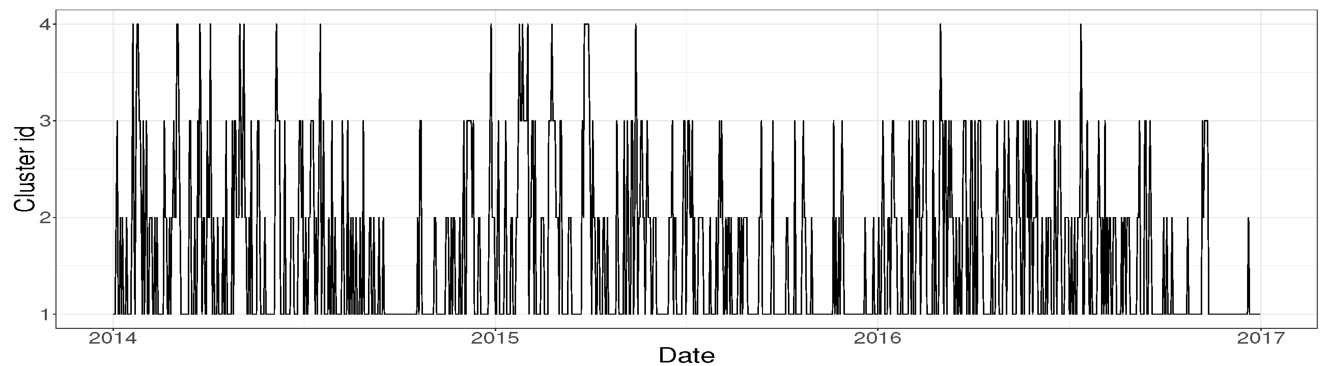
Hierarchical classical clustering has been performed over the normalized dataset for Wf1 data, by using Ward’s method [14] and Euclidean distance, as all variables are numerical. The resulting dendrogram is shown in Figure 5 and Calinski-Harabasz index [15] has been optimized to determine the resulting number of clusters. A cut in 4 clusters is suggested. CPGs and TLPs build over the resulting clusters apparently show good results and provide clusters with quite clear interpretation. However, when the daily classification of the wind turbine is temporally plotted, as we can see in Figure 6, the clusters change chaotically from one day to another, as if the wind turbine experimented pattern changes asynchronously along time. This pattern seems not to be realistic and makes difficult the understanding of the wind turbine operation regime. 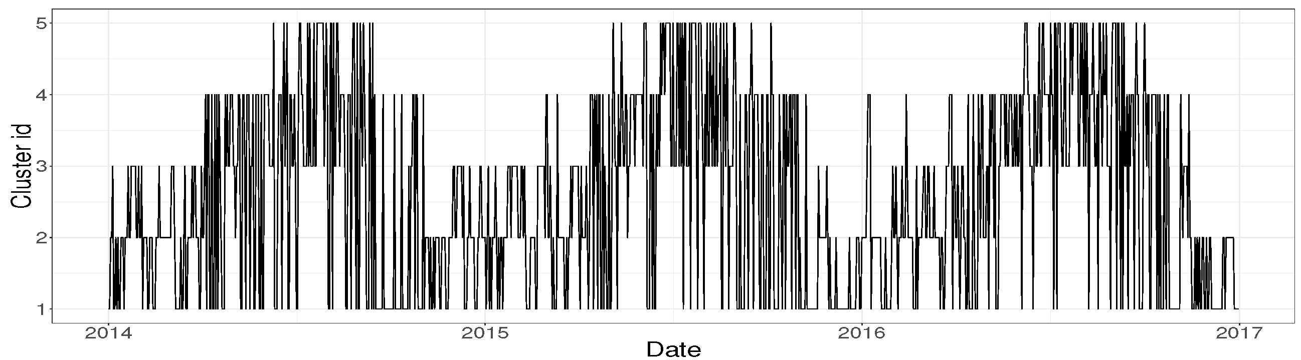In Figure 7 it can be seen the corresponding temporal evolution of the daily classification of the wind turbine operation, obtained by applying the local analysis methodology proposed in Section 4.5. It is clear that the proposed method is able to capture much better the intrinsic stationarity of the aero-generation phenomenon.

2.7. Validation with Additional Wind Farms

Based on these evidences, we extend the application of the proposed local analysis methodology to the rest of the wind farms.

The same procedure was applied to the gearbox system failures for the other two wind farms. Results are shown in

Table 6. Results for a group size of 4 for ’codes2’ and ’moncayuelo’ wind farms; includes the probability generated by an expert per group and the real number of maintenance events observed.

Wind Farm	Group Id	Nr of Turbines	Expert Probability			Maintenance Events
			Mean	Median	sdv	Count	Mean	Median	sdv
moncayuelo	1	7	0.14	0.14	0.09	8	1.14	1.15	2
	2	20	0.29	0.26	0.16	46	2.3	1.53	2
	3	4	0.16	0.15	0.04	16	4	2.45	4
	4	1	0	0	0	0	0	0	0
codes2	1	37	0.24	0.20	0.15	49	1.32	1.29	1
	2	9	0.11	0.10	0.09	9	1	0.84	1
	3	3	0.67	0.7	0.15	4	1.33	1.41	2
	4	1	0.2	0.2	NA	1	1	NA	1

. For each wind farm, turbines have been clustered according to the proposed methodology in 4 clusters. In the Table, the column “Group Id” indicates the class identifier. The number of turbines involved in each of these classes is shown in column “Nº of turbines”. “Expert probability” columns provide the mean, median and standard deviation of the probability of failure estimated by the expert for the turbines of the class, whereas columns “Maintenance events” contains statistics related to the real number of maintenances required in the turbines of each group.

In the first wind farm, moncayuelo, we can see that group 2 has the higher probability of failure given by the expert (mean and median), besides the number of repairs (mean and median) is also the highest of the four groups. Therefore, this group will contain the unhealthiest turbines. In group 3, even though the expert determines an intermediate failure probability, the amount of repairs is high, indicating that it is a group that could also be considered as unhealthy (or close to) when creating a classification of turbines. In group 1, both the expert and the number of repairs are among the lowest, so it groups turbines in excellent condition. Group 4 contains the turbine in the best condition of the farm since the number of repairs is zero and also the expert has assigned the lowest value (0).

In the second wind farm, codes2, group 1 contains the turbines in an intermediate state of health according to both failure probability of the expert and repairs. Group 2 has the turbines in better condition according to both criteria. In group 3 we have the turbines with the highest failure rate and that the expert also considers that the probability of failure is high. Finally, group 4 contains a turbine that does not resemble any of the other groups. Even if it is not considered as damaged, the turbine belonging to this group needs to be further analyzed to clarify whether it is another mode of operation or hides some other problem.

3. Discussion and Future Work

Identifying health status of wind turbines is a severe problem that cannot be tackled by using simple data analysis methods because the interactions between the factors impacting in particular kind of failures are too complex. As it has been seen in the paper, the plain hierarchical clustering is not able to tackle the stationarity involved in the process.

The main contribution of our system is the proposal of an intensive data-driven methodology able to automatize the identification of groups of turbines with similar behaviors, that can support the company staff in selecting a reduced number of representative turbines for in situ inspections. This solves a critical issue in the company, related to human and economic resources involved.

The proposal provides a data-driven methodology based on a strategic combination of SOM, hierarchical clustering, post-processing and simplex-based matching, that was resulting successful in grouping turbines according to its healthy state for different group sizes providing an understanding of this status. The groups contain turbines with a similar number of maintenance interventions, also in accordance with the expert evaluation, validating that the groups are well derived.

To do that, we develop a strategy based on the comparison of the centroids of the local BMUs, which facilitates the characterization of each turbine as a vector of operational status (the N local centroids). This allows a further re-grouping of turbines by merging in groups those that behave similarly as a whole, i.e., have similar vectors of operational regimes. The introduction of CPG and TLP as interpretation oriented tools was of major importance to elicit the meaning of the patterns identified and supporting the final diagnoses made by the experts about operational regimes of the turbines.

The importance of our proposed method relays in the fact that this initial clustering of turbines can be done automatically, generating 3 (or more) groups, each one with turbines in a similar healthy state. Thanks to the application of interpretation tools such as CPG and TLP, it has been possible to understand the information captured by the SOM, clearly identifying at least four different types of turbine operating modes that directly impact in energy production rates. Therefore, the human expert can focus his/her work only on a subset of turbines, according to the problem to be solved. Thus we save precious and expensive time, especially when large farms or many different farms have to be handled by the same specialist.

Moreover, our system allows for identifying interactions in the behavior of the variables involved, from an N-dimensional analysis and particular areas of some problematic turbines. Therefore, after the identification of the unhealthy classes, in which the use of CPG and TLPs is supporting the conceptualization of the clusters, our system allows monitoring the time evolution of any turbine, by visualizing how their clusters/centroids evolve and identifying if they are moving towards the distribution of an unhealthy class. This automatic process is of paramount importance to reduce costs and handle an important number of turbines and wind farms.

The process has been automatized and scaled to be in production in a real company, and it provides a helpful framework to identify a reduced set of turbines to be inspected in situ.

The proposed method has also been applied to two additional wind farms to validate their real usability.

To the best of our knowledge, this is the first exploratory work that combines SOM, clustering based on BMUs and turbine characterization through CPG and TLPs altogether. Many aspects would need an in-depth, and other possibilities can be considered. For example, the clustering algorithm used on BMUs has a real effect on the final clusters, and also the way we group turbines based on the distance between centroids by means the simplex algorithm. Here, several measures of distance/correlation could be used and will be explored in future work. Also, the variables considered for the problem to be modeled could be automatized through a feature selection algorithm, instead of using a human expert. This feature selection algorithm will have a significant effect on the result. Hence an in-depth investigation should also be carried on. Finally, the optimum number of clusters derived in Section 4.5 could also be determined by evaluating the quality of the clusters generated in each turbine. Possible relevant metrics to do so are the Davies–Bouldin index [15,16] and the Silhouettes index [17]. These metrics should be computed for each dendrogram, exploring a reasonable range for the number of clusters, and for each turbine individually. Then, we could calculate the average for each metric for turbines within the same amount of clusters. The trade-off between the two results could be used to determine the optimal number of clusters to be applied for all the turbines. Regarding the CPG and the TLP, there is work in progress to implement several automatic criteria to built the TLPs from some overlapping indicators between the local distributions of variables inside each class. The degree of overlapping between classes will determine the three levels of each variable, the assignment of a color to each cell of the TLP. The automatic interpretation of the patterns would also be included in the standard automatic processing of the wind farms to define strategic in situ inspections.

4. Materials and Methods

4.1. Data

The SCADA data used in this work follows the IEC 61400-25 format [18]. The data was gathered via an OPC (OLE for Process Control) [19] with frequencies of 5 or 10 min, for a rich set of variables. Each sensor usually provides minimum, mean, maximum and standard deviation values for each variable.

The dataset is stored in a local database, which has been recording values from the SCADA over the years. The dataset is structured as a table, with the time evolution in rows and sensors variables in columns. The wind farms used in this work are detailed in

Table 7. Summary of the dataset used in this work. The Table shows the number of wind turbines, number of years of historical data available, the frequency of each wind turbine, number of variables, number of events (alarms in this case) and the total number of registers evaluated by each experiment. Each experiment corresponds to a different wind farm.

Turbine	Number of Turbine	Years	Rows/Year	Variables	Triggered Alarms	Total Registers Evaluated
Wf1 3MW (confidential)	16	3	52.560	181	709.972	2.522.880
Acciona Wind Power	50	3	52.560	163	80.194	7.884.000
AW-1500 ’codes2’
Acciona Wind Power	32	4	52.560	142	21.742	6.727.680
AW-1500 ’moncayuelo’
Total	98	10			811.908	17.134.560

.

According to the fault to be detected, an expert decides which variables will be used to analyze the system. In this work, gearbox problems will be focused because, as already mentioned above, it is one of the main important turbine systems, being the responsible for expensive maintenance costs due to its components. These variables could also be obtained through different Feature Selection algorithms see

Table 8. Different Feature Selection algorithms used in [20] to identify relevant variables, as an alternative to expert-based variables selection.

Algorithm	Author
Mutual Information Feature Selection (MIFS)	Battiti [21]
Conditional Mutual Information (CMI)	Cheng et al. [22]
Joint Mutual Information (JMI)	Yang and Moody [23]
Min-Redundancy Max-Relevance (mRMR)	Peng et al. [24]
Double Input Symmetrical Relevance (DISR)	Mayer and Bontempi [25]
Conditional Mutual Info Maximisation (CMIM)	Fleuret [26]
Interaction Capping (ICAP)	Jakulin [27]

, although according to previous works the variables selected by an expert give excellent results [20]. All the analysis carried on will be in daily scale.

Maintenance interventions directly related to the gearbox have been kept on the database, as well as a failure probability analysis obtained by an expert after his analysis of oil and temperature. This information will be used to evaluate the quality of the groups generated by our proposed procedure.

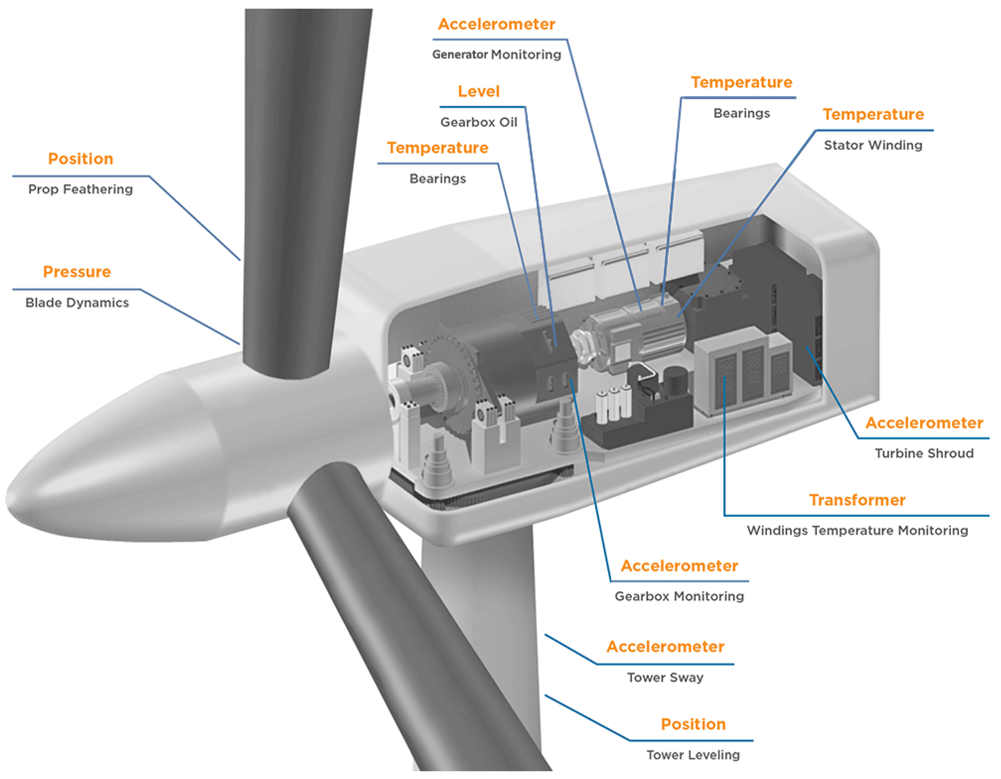
The variables selected by an expert as relevant for the gearbox operation are introduced below. Figure 8 provides an overview of a wind turbine and these variables:

• Power The power generated by the wind turbine in KW.
• GearboxOilTemp The temperature of the gearbox oil , in degree Celsius.
• GearboxBearingTemp The temperature of the gearbox bearing (output side) , in degree Celsius.
• AmbientTemp The external temperature of the environment, in degree Celsius.
• RotorSpd The speed of the rotor main shaft before gearbox, in revolutions per minute (RPM).
• WindSpd The wind speed in m/s measured by the anemometer at the wind turbine’s nacelle.

Additionally, a new variable is internally created to evaluate the results, as a non-linear combination of two of the variables provided by the SCADA system. It reflects a parameter often used by experts in the interpretation of the health status of wind turbines and enhances the interpretation process.

• PowerWind_ratio The ratio of the Power variable divided by the wind speed.

As we try to discover abnormal behaviors and wind turbines are different among them, data is normalized to Z-score to eliminate wind turbine heterogeneity from the analysis. However, the normalization factors must be saved to reconstruct the original variables for graphical analysis. The extreme values (outliers) are set to NA, and then the rows that contain any variable with NA is removed since it represents less than the 5% of the total number of registers. Further analysis focalized to registers with missing data are in progress. A complete set of guidelines to be taken into account in preprocessing can be found in [28].

4.2. Methodology Overview

Self organizing maps (SOM), introduced by T. Kohonen [10], is a type of unsupervised ANN mainly employed in feature reduction and data visualization. This neural network has been used in many different kinds of applications, ranging from speech processing (the original field in which Kohonen presented it, [29]), seismic data analysis [30], image processing [31], genetic data [32], etc.

The SOM uses an unsupervised algorithm based on competitive learning, in which the output neurons compete with each other to be activated, with the result that only one is activated at a given time. The result is that the neurons are forced to organize themselves in a specific manner which generates the map. Usually, the nodes of the network are organized in a regular 2D space, in which each unit (neuron) in the input layer is connected to all neurons in the output layer. Each connection has a weight and, this weight will be adjusted during the process with the aim of mapping input patterns to the output 2D structure by preserving the topology. This means that points that are near each other in the multiple dimensional input space will be mapped to nearby map units in the 2D SOM map. Therefore, SOM can be used as a cluster analyzing tool of high-dimensional data. Also, SOM has the ability to generalize, which means that the network can recognize or characterize entries it has never seen before. A new input vector is assimilated with the unit on the map to which it is mapped to.

Self Organizing Maps have been used in the condition monitoring area on several occasions. Some works [13,33,34,35,36] use the map generated with all turbines to explore how the data is distributed by performing an analysis in the unified distance matrix (U-matrix), which is a way to visualize the distances between neurons. Other works go one step further by applying clustering on the U-matrix to find patterns on the map [13,36,37,38,39].

In our case, we go beyond the classical approach proposed in the literature by adding a second step of the analysis in which the SOM is subdivided into sub-maps local to each one of the turbines (see details in Section 4.5 to find the behavioral patterns shown by every single turbine). A further regrouping of these patterns in a final step (see Section 4.6) leads to a global grouping of these patterns

The interest of this approach is to get an in-depth comprehension of which turbines are in better or less operational mode and helps to decide which specific turbines have to be inspected.

For this purpose, understanding of the meaning of both global or local clusters become critical.

The results of the clustering methods in general, including SOM, require some further processing to understand which are the meaning of the discovered clusters and to properly conceptualize them [12]. Classically, U-Matrix visualizations are used to interpret SOM results, and also projections of observed variables onto the SOM map. Another visual output derived from the SOM map are the heatmaps of the variables which is done individually for every single variable and provide a way of identifying the areas of the SOM map associated higher and lower values of the variable. However, it is difficult to get a global perspective, as these tools analyze every single variable separately.

Being a real application that needs to provide support to a real strategic decision in the company, getting a global overview of what the patterns are telling us regarding turbines’ health is of vital importance. Thus, specific interpretation-oriented tools are introduced to support the understanding of the patterns discovered by the SOM (see Section 4.7). A crucial step in this unsupervised data-mining process is to transform the results of the SOM into understandable knowledge for providing effective decision-making support [40].

The Figure 9 contains a diagram of the whole proposed process, also in the following sub-Sections, specific details on each one of the steps of the proposed process are provided.

4.3. Software

The software selected to generate the model and analyze the data is R version 3.4.3. The library needed to generate the SOM maps is Kohonen package by Ron Wehrens and Johannes Kruisselbrink [41]. To create the clusters the base package hclust by Fionn Murtagh and Pedro Contreras [42]. The CPGs and TLPs are generated with by the KLASSv18 proprietary software by Karina Gibert [43] which is a data mining software, specifically designed to introduce expert knowledge and semantics into clustering processes of heterogeneous data and contains a specific module of interpretation oriented tools. Finally, the Simplex method implemented into the turbine’s centroids pair computation is provided by the linprog package by Arne Henningsen [44]. To reproduce and repeat the results the same dataset must be used and also the same random seed, in our case, we defined the number 1 as the random seed (set.seed(1) in R).

4.4. Selection of the Optimal SOM Size

The size of the map depends to a large extent on the dimension of the input data. According to [13], the initial map size should contain $n=\lceil 5\sqrt{R}\rceil$ neurons, where R is the number of registers and the result is finally rounded up (ceiling). However, [33] indicates that it is possible to obtain the optimal dimensions through an exploratory way by using the U-Matrix [45].

In this work, we will use some metrics to set the map size. These will allow us to automate this step. It is known that larger map sizes produce over-fitting because fewer records are associated with each neuron, and hence each neuron specializes in a particular record, which is not the goal of the SOM [46]. However, a too small map size would not end up collecting the particular behavioral records that are not associated with isolated neurons, considered as outliers. That is why a trade-off has been sought using the metrics described in [10,47]. These metrics are the Topographic error (TE) and the Quantization error (QE), the first one increases as the map gets bigger meanwhile the second one decreases. With these two metrics behaving in opposite ways, a balanced size could be achieved between the two of the different maps generated.

The TE is calculated by analyzing each input register and considering the 1st and 2d best matching unit (BMU). If they are not adjacent, the TE is increased by 1, otherwise is kept at its previous value. When all the registers have been analyzed, the total value is divided by the total number of registers obtaining its mean. The TE value increases if the map becomes larger, due to the increase in the number of units and therefore the decreasing on the probability of having adjacent 1st and 2d BMUs.

On the contrary, the QE decreases as the map become larger, since it quantifies the distance from each register to the assigned BMU. Hence, the larger the map is, the higher the resolution and the smaller all these distances because there is a higher chance that the register comes closer to its assigned BMU.

To find the best size for the SOM, the metrics mentioned above are first of all normalized in a range between 0 and 1. Then, the (normalized) values of the two metrics are obtained for several SOM versions with different sizes. Finally, the cut-off point between the two crossing curves of TE and QE will be used as the best size for the SOM. These metrics do not have a linear behavior, so the cut-off point substantially varies depending on the explored size of the SOM. Experimental tests showed that these metrics have an exponential behavior, one with negative decay while the other with positive decay. A linear shape may indicate over-fitting, and a different range of sizes should be tested, usually smaller than the previous ones.

4.5. Generating Sub-Maps by Turbine

In the previous Section, a method to derive an optimal size of the SOM for a given dataset is proposed, based on a trade-off between two metrics, evaluated in a range of different sizes.

In this Section, a proposal to subdivide the SOM map into sub-maps local to each turbine is presented.

First of all, for each turbine, a list of BMUs are obtained. This procedure is done by first selecting the registers from the original dataset that corresponds to the target turbine and then, the BMU of each of those registers is identified in the SOM results. The selected subset of BMUs provides a sub-map of the same size as the original, but with a subset of visible neurons (those activated by the registers of the target turbine) and invisible neurons (the neurons without registers of the target turbine). So, by comparing sub-maps of different turbines among them, it is possible to discover turbines sharing the same activation zones, which are candidates to be grouped. Identifying which turbines show common patterns of SOM activation is easy from a graphical point of view. However, to implement efficiently in a production phase the procedure in the daily activities of the company, this step has to be performed automatically.

The main challenge is that the specific BMUs activated by two similar turbines are not exactly the same, even if they are in close neighborhoods. Thus a local clustering of the BMUs activated by a single turbine and a centroids-based representation of these clusters will provide a synthetic view of the activation areas of a given turbine and will allow further comparisons to detect groups of similar turbines automatically. The clustering algorithm used in this work is based on the Hierarchical clustering [48].

4.6. Re-Grouping Turbines

Provided that in this particular context all turbines of a given wind farm are technologically similar, it has been seen that most of them show the same number of clusters N. This is very interesting because it enables pairwise comparisons between turbines in terms of Euclidean distances between their centroids-vector derived in Section 4.5.

However, the cluster identifier of a particular operational regime (like optimal production, for example) can change from one turbine to another one, since discovered clusters are automatically named by the algorithm. Thus, given a pair of turbines T and T’, cluster 1 in turbine T might point to a different scenario than cluster 1 in turbine T’. This means that even though the behavior of a certain turbine can be synthesized by a vector of N centroids, one per cluster, distances between pairs of turbines cannot be directly computed. The Simplex method [49] is introduced for this purpose, to find the permutation of centroids of turbine T’ that minimize the total distance to the centroids of turbine T ($d_{min}(T,T^{\prime })$). The combination of centroids between turbines that generates $d_{min}(T,T^{\prime })$ is the optimal one, and provides the correspondence between clusters in T and those in T’. The distance between the two turbines T and T’ is then defined as $\frac{d_{min}(T,T^{\prime })}{N}$ , that is, the average distance between pairwise centroids between T and T’.

Repeating this procedure with all distinct pairs of turbines a square (symmetric) distance matrix between turbines is obtained in Figure 4. Each row or column in Table 4 identifies a turbine.

Based on this distance matrix, a further grouping of similar turbines can be pursued. A density-based like clustering process is performed by setting a threshold p-threshold that determines the neighborhood of a certainly visited wind turbine and all other wind turbines inside this neighborhood are included in the same cluster. The p-threshold must be a positive real number from 0 to 1 which defines the proportion of the total distance range on the table. The process starts by finding the cell containing the smallest distance (v-min) in the table. The row that contains this cell identifies the first turbine T visited and its distances to the other turbines. Each column in the matrix represents another turbine (namely T’). All turbines T’ such that $d(T,T^{\prime })<\mathit{v}-\mathit{min}+\mathit{p}-\mathit{threshold}$ will be added together in the cluster $C_T$. After the first group is set, the rows and columns identifying the turbines of it are eliminated from the distance matrix and the process is repeated to determine the next group, until all the turbines are clustered in some group.

Since the distance matrix is quadratic in the number of turbines, and this is not a huge dimensionality, this process can be repeated with several values of p-threshold, starting by a small value like (0.1) and increasing by steps for a posteriori evaluation of the preferred p-threshold. Higher values of p-threshold generate fewer groups which are more general. Lower values of p-threshold give more groups which are more specific.

In order to check the validity of the groups generated by this procedure, they will be compared with the failure probability generated by the experts in in situ inspections, as indicated in Section 4.1 (qualitative evaluation). Also, the maintenance and failure events of the turbines will be used by calculating the statistics of these indicators to check that the groups contain turbines with similar problems (quantitative evaluation).

4.7. Post-Processing the Results of Self-Organizing Maps for a Better Understanding of the Discovered Patterns

As mentioned before, a couple of tools are introduced as a post-processing of the SOM results and the hierarchical clustering processes used in this work. Both of them were designed with the aim of helping experts to conceptualize and label the resulting classes. Originally, CPGs and TLPs [50] were designed in the context of hierarchical clustering. In this paper, for the first time, they are used on clusters induced from a SOM network.

The CPG is based on a simple idea but resulted very powerful in previous real applications where clusters understanding was critical. It is based on placing in a single panel the conditional distributions of the variables with regards to the clusters. Columns correspond to variables and rows to clusters. Histograms or box-plots are displayed for numerical variables and bar-charts for qualitative ones [50]. It allows to identify particularities of classes in regards of specific variables. Basically, the inherent nature of the clustering is based on the idea that observations group in different clusters because, on the one hand, they can be distinguished by some characteristic behaving differently in one or other cluster and, on the other hand, they must share some distinctive commonalities with the other observations in the same cluster. The CPG permits a quick analysis to identify these distinctive commonalities.

One step forward in the level of abstraction of the interpretation-support tool is the TLP. TLP is a symbolic post-processing of the clustering results proved extremely useful and well-accepted by domain experts in several real applications [11,50]. TLP exploits the association between the traffic light colors and the main central trend of the variables in every class to help the expert to understand the clusters and to support the conceptualization. In fact, it can be visually built upon the image proposed by the CPG, or automatically computed in terms of overlapping measures among the conditional distributions of a variable in the several clusters. The main issue is that deciding whereas high values of the variable will be assigned red or green color is associated with the semantics of the variable itself, so bringing semantics into the picture of the interpretation process in a formal way. In this particular application, for example, producing high levels of power is better than low production, and that is why high levels will be associated with green and low with red color. In [12] an extension to annotated-TLP is presented, where the basic color of the cell is desaturated with a darker tone proportionally to the variability inside the class, so the expert is able to catch, from the picture, which are the cells which they can trust their decisions.

In this work, both CPG and TLP have been built to understand the patterns resulting from the hierarchical clustering of the SOM cell prototypes (BMU), as well as to understand the patterns resulting from the local analysis of each specific turbine when clustering their positions in the SOM map.The software KLASSv18 has been used for this purpose [43].