A Load-Shedding Model Based on Sensitivity Analysis in on-Line Power System Operation Risk Assessment

Abstract

The traditional load-shedding models usually use global optimization to get the load-shedding region, which will cause multiple variables, huge computing scale and other problems. This makes it hard to meet the requirements of timeliness in on-line power system operation risk assessment. In order to solve the problems of the present load-shedding models, a load-shedding model based on sensitivity analysis is proposed in this manuscript. By calculating the sensitivity of each branch on each bus, the collection of buses which have remarkable influence on reducing the power flow on over-load branches is obtained. In this way, global optimization is turned to local optimization, which can narrow the solution range. By comprehensively considering the importance of load bus and adjacency principle regarding the electrical coupling relationship, a load-shedding model is established to get the minimum value of the load reduction from different kinds of load buses, which is solved by the primal dual interior point algorithm. In the end, different cases on the IEEE 24-bus, IEEE 300-bus and other multi-node systems are simulated. The correctness and effectiveness of the proposed load-shedding model are demonstrated by the simulation results.

1. Introduction

With the continuous development of the economy, the scale of power systems is getting larger, and their structure is getting increasingly complicated. In recent years, large-area power failures have frequently occurred and have caused huge economic losses [1,2]. In order to eliminate the potential risks and ensure the operational safety and reliability of power systems, the risk identification, risk monitoring and risk management based on operation risk assessment have received great attention, which has become one of the major tasks of urban power grid management [3,4]. The power system risk assessment is the comprehensive measurement of possibility and consequences. The probability and consequences of different scenarios are directly related to the operation state and external environment, which are both time-varying and stochastic. Besides that, “N-1”, “N-2” and other failure modes will lead to a great number of fault scenarios, which should be evaluated within a short period of time (such as 30 min). Thus, the power system risk assessment should be carried out on-line to ensure its accuracy and timeliness.

The load loss caused by failures of power equipment is an important aspect of risk consequences, which is also one of the core contents of the power system operation risk assessment. When power equipment failures lead to overloading of branch power flows, load-shedding models are applied to calculate the quantity of load reduction caused by the branch overload. As the number of the failure scenarios being considered is large, many scenarios, especially the multiple fault scenarios, usually cause the overload of branch power flows. Then a load-shedding model is applied to eliminate the overload of each branch. Thus, the computation speed of load-shedding model is the key to promote the calculation efficiency of operation risk assessment and achieve the on-line evaluation.

The traditional load-shedding methods include: random load reduction method; average load reduction method; bus importance-based load reduction method [5]; nearby load reduction method [6,7,8]; optimum load reduction method [9,10,11,12,13]. The random load reduction method and average load reduction method refer to cutting down the load in the load reduction region randomly and averagely, respectively. The amount of load reduction calculated by these two methods is quite different from the practical situation, which makes them non-applicable in power system operation risk assessment. In [5], the load weight was obtained by trial and error, so the load buses are classified by their importance. In this way, the least important load buses are firstly cut down, then the less important load buses, and so on. In [6], the adjacency principle was proposed to obtain the nearest load bus, in this way the load-shedding region was achieved, which is the range of target bus to cut down load. Reference [7] obtained the load bus set by setting the “bus degree value” to get the load buses closest to the failed equipment. Reference [8] calculated the distance of each load bus to the failed equipment regarding the network topology, in order to cut down the loads of the relatively close buses. In [9], by comprehensively considering the importance of each bus and their distance to the failed equipment into consideration, a direct current power flow model was used to calculate the load-shedding results. In [10,11,12], the optimal power flow model was applied to rapidly determine the load-shedding region and calculate the total amount of load reduction. Reference [13] calculated the contribution coefficient and distribution factor of the power flow from generators, load buses and transmission lines. Then the optimized load-shedding region is achieved. All these traditional load-shedding methods used global optimization, which takes all the load buses into consideration and had complex constraint conditions. This will lead to a reduction of the speed of calculation, which makes it hard to meet the requirements of timeliness in on-line operation risk evaluation.

In fact, when power equipment failures cause load reductions, the load buses which are far from the failed equipment have little influence on reducing the power flow on overloaded branches. In other words, searching for the target load buses in the global scope is not necessary. The “bus degree value” [7,14] and distance between the load buses and failed equipment calculated by a power flow tracing method [8,15,16,17] are applied regarding the physical distance and topological distance, respectively. However, the physical distance and topological distance cannot explain the electrical coupling relationships between power equipment. The load reduction region should include load buses which are filtered by comprehensively considering the physical distance and electrical coupling relationships.

As mentioned above, defects of the present load-shedding models are as follows: firstly, traditional load-shedding models use global optimization to determine the load reduction region. This will cause multiple variables, huge computing scale and other problems, which would greatly influence the calculation efficiency. Secondly, the traditional adjacency principle regarding the physical distance and topological distance cannot consider the electrical coupling relationships, which means the target load buses include too many useless buses which may have little influence on reducing the power flow on overload branches. Finally, the calculation speed of traditional load-shedding models cannot meet the requirements of timeliness, which makes it hard to be applied in on-line power system operation risk assessment.

Aiming at solving the problems of the present load-shedding models, this manuscript proposes a load-shedding model based on sensitivity analysis. In Section 2, the principles of sensitivity analysis are introduced, based on which the load reduction region is achieved. This load reduction region can be better applied to the situation where the failed equipment causes several overloaded branches. In Section 3, based on the obtained load reduction region, by comprehensively considering the importance of load bus and adjacency principle regarding the electrical coupling relationship, a load-shedding model is established to get the minimum value of the load reduction from different kinds of load buses. The primal dual interior point method is used to solve the proposed load-shedding model. In Section 4, the IEEE 24-bus system, IEEE 300-bus system and other multi-node systems are applied to verify the validity and correctness of the proposed load-shedding model. Finally, conclusions are drawn in Section 5.

2. Filtration Method of Load Reduction Region Based on Sensitivity Analysis

The essence of sensitivity analysis in calculating the load reduction region is to calculate the partial differential of branch power flow on input power of each bus node [13,18,19,20,21,22]. Reference [18] showed the application of sensitivity analysis through Laplace transform and the use of load-damping coefficients for frequency regulation. Reference [19] showed how the rate of change of voltage with respect to active power can be used to identify the sensitive buses for load shedding. In [20], the application of the sensitivity analysis method in static voltage stability analysis of power systems is summarized, and various sensitivity indexes are discussed. In [21], by analyzing the calculation process of available transfer capability based on direct current distribution factors and according to the variation of key constrained lines or constrained tie line power flow determining available transfer capability after nodal power varied, the sensitivity between available transfer capacity and nodal power can be obtained. In [22], an overview of sensitivity analysis was proposed, which provides an easy way to understand what the sensitivity analysis consists of. Thus, the power flow sensitivity index reflects the changing degree and trend of changes on branch power flow from the small changes of the input power on bus nodes. If the power flow sensitivity indexes of an overloaded branch on some bus nodes are high, it means that the input power of these bus nodes have great influence on the power flow of this branch. The reduction of input power on these bus nodes can effectively eliminate the overload circumstances. By calculating the power flow sensitivity of each branch on each bus node in the system, the electrical coupling relationships between different power equipment can be reflected. In this way, a bus collection can be obtained which can truly reduce the power overload on the target branch. In the next section, the fundamental principles of sensitivity analysis are discussed, based on which the calculation method of load reduction is proposed.

2.1. Fundamental Principles of Sensitivity Analysis

Sensitivity analysis includes two parts: (1) the sensitivity of bus node input power on its voltage angle and amplitude; (2) the sensitivity of branch power flow on bus node voltage angle and amplitude. Then, the sensitivity of branch power flow on bus node input power can be obtained by uniting these two kinds of sensitivity.

• The sensitivity of bus node input power on its voltage angle and amplitude

The sensitivity of bus node input power on its voltage angle and amplitude, which is abbreviated as J in this manuscript, is calculated as:

$$\left[\begin{array}{c}\Delta P\\ \Delta Q\end{array}\right]=J\times \left[\begin{array}{c}\Delta \delta \\ \Delta V\end{array}\right]=\left[\begin{array}{cc}{H}_1& N_1\\ K_1& L_1\end{array}\right]\times \left[\begin{array}{c}\Delta \delta \\ \Delta V\end{array}\right]$$

(1)

where H₁ is a matrix of $(n-1)\times (n-1)$, whose element $H_{1\_ij}$ means the partial differential of the active power on bus node i to the reactive power on bus j, calculating as $H_{1\_ij}=\partial P_i/\partial Q_j$; K₁ is a matrix of $m\times (n-1)$, whose element $K_{1\_ij}$ means the partial differential of the reactive power on bus node i to the voltage angle of bus j, calculating as $K_{1\_ij}=\partial Q_i/\partial {\delta }_j$; N₁ is a matrix of $(n-1)\times m$, whose element $N_{1\_ij}$ means the partial differential of the active power on bus node i to the voltage amplitude of bus j, calculating as $N_{1\_ij}=\partial P_i/\partial V_j$; L₁ is a matrix of $m\times m$, whose element $L_{1\_ij}$ means the partial differential of the reactive power on bus node i to the voltage amplitude of bus j, calculating as $L_{1\_ij}=\partial Q_i/\partial V_j$; P_i and Q_i refer to the active power and reactive power on bus node i, respectively; ${\delta }_j$ and $V_j$ refers to the voltage angle and amplitude of bus j, respectively; n and m refer to the number of total nodes and PQ nodes, respectively.

• The sensitivity of branch power flow on bus node voltage angle and amplitude

The sensitivity of branch power flow on bus node voltage angle and amplitude, which is abbreviated as $J_s$ in this manuscript, is calculated as:

$$J_s=\left[\begin{array}{c}{J}_{s1}\\ \dots \\ J_{sd}\end{array}\right]$$

(2)

where $J_{s1}$ and $J_{sd}$ refer to the sensitivity of power flow on the 1st and dth branch to the voltage angle and amplitude of each bus node, respectively; d refers to number of the over-load branches.

More concretely, the sensitivity of power flow on the fth branch to voltage angle and amplitude of each bus node, which is abbreviated as $J_{sf}$ in this manuscript, is calculated as:

$$\left[\begin{array}{c}\Delta P_f\\ \Delta Q_f\end{array}\right]=J_{sf}\times \left[\begin{array}{c}\Delta \delta \\ \Delta V\end{array}\right]=\left[\begin{array}{cc}{H}_{2\_f}& N_{2\_f}\\ K_{2\_f}& L_{2\_f}\end{array}\right]\times \left[\begin{array}{c}\Delta \delta \\ \Delta V\end{array}\right]$$

(3)

where $H_{2\_f}$ is a matrix of $1\times (n-1)$, whose element $H_{2\_fj}$ means the partial differential of the active power on branch f to the voltage angle of bus j, calculating as $H_{2\_fj}=\partial P_f/\partial {\delta }_j$; $K_{2\_f}$ is a matrix of $1\times (n-1)$, whose element $K_{2\_fj}$ means the partial differential of the reactive power on branch f to the voltage angle of bus j, calculating as $K_{2\_fj}=\partial Q_f/\partial {\delta }_j$; $N_{2\_fj}$ is a matrix of $1\times m$, whose element $N_{2\_fj}$ means the partial differential of the active power on branch f to the voltage amplitude of bus j, calculating as $N_{2\_fj}=\partial P_f/\partial V_j$; $L_{2\_fj}$ is a matrix of $1\times m$, whose element $L_{2\_fj}$ means the partial differential of the reactive power on branch f to the voltage amplitude of bus j, calculating as $L_{2\_fj}=\partial Q_f/\partial V_j$; P_f and Q_f refer to the active power and reactive power on branch f, respectively.

When judging a branch whether it is overloaded or not, its apparent power is compared with its transmission limit. Thus, the sensitivity of apparent power on branch to bus node voltage angle and amplitude should be deduced, shown as:

$$\Delta |S_f|=\left[\begin{array}{cc}(P_f\frac{\partial P_f}{\partial \delta }+Q_f\frac{\partial Q_f}{\partial \delta })/|S_f|,& (P_f\frac{\partial P_f}{\partial V}+Q_f\frac{\partial Q_f}{\partial V})/|S_f|\end{array}\right]\times \left[\begin{array}{c}\Delta \delta \\ \Delta V\end{array}\right]$$

(4)

where $\left|S_f\right|$ refers to the apparent power of branch f.

Power factor angle ${\theta }_f$ of branch f can be applied to simplify Equation (3). Considering $\cos {\theta }_f=P_f/\left|S_f\right|$ and $\sin {\theta }_f=Q_f/\left|S_f\right|$, Equation (3) can be converted into:

$$J_{sf}=\left[\begin{array}{cc}(\cos {\theta }_f\times H_{2\_f}+\sin {\theta }_f\times K_{2\_f}),& (\cos {\theta }_f\times N_{2\_f}+\sin {\theta }_f\times L_{2\_f}\end{array})\right]$$

(5)

• The sensitivity of branch power flow on bus node input power

Uniting Equations (1)–(3), the sensitivity of the power flow on branch f to the input power of each bus node, which is abbreviated as $T_f$, can be calculated as:

$$\Delta |S_f|=J_{sf}\times \left[\begin{array}{c}\Delta \delta \\ \Delta V\end{array}\right]=J_{sf}\times J^{-1}\times \left[\begin{array}{c}\Delta P\\ \Delta Q\end{array}\right]=T_f\times \left[\begin{array}{c}\Delta P\\ \Delta Q\end{array}\right]$$

(6)

2.2. Filtration Method of Load Reduction Region

From Section 2.1, the sensitivity of the power flow on each branch to the input power of each bus node can be calculated. It is obvious that this sensitivity can be larger or less than zero:

(1)

If the sensitivity of the power flow on branch f to the input power of bus node j is larger than 0, it means that the input power of bus node j is negative. Thus, this bus node j is a generator node or an equivalent power supply node from external power grid.

(2)

If the sensitivity of the power flow on branch f to the input power of bus node j is less than 0, it means that the input power of bus node j is positive. Thus, this bus node j is a load node.

If the failed equipment causes power overload on some branches, it means that some loads are transferred to these overloaded branches because of the changes of network structure. According to the power balance principle, in this situation, firstly the generators output should be adjusted to meet the equilibrium between the demand side and the supply side. If the additional power requested by load in the node is greater than the available spinning reserve of the directly connected generator(s), from the perspective of the demand side, the loads on other nodes should be reduced to satisfy the generator maximum outputs. After this step, if the overloading situation persists, loads on other buses should be reduced through some load-shedding model, and the generator output should be reduced automatically. This manuscript is designed from the demand side, which is on the basis that all the generators in the system are adjusted automatically. The amount of load shedding results do not contain the changes of generator outputs, so the generator buses can be excluded from the load shedding region. Besides that, for those load nodes, the bigger the absolute value of its corresponding sensitivity is, the more effective it can reduce the power on the overloaded branches. So it is necessary to filter the load nodes whose absolute value of its sensitivity are relatively larger, in which way the optimized load reduction region can be obtained.

The traditional filtration methods include threshold value method [23], equal proportion filtration method [24], and K-mean filtration clustering method [25]. The threshold value method cannot adapt to the changes of power system because it is empirical, even though this method is simple and easy to operate. The equal proportion filtration method refers to select the targets by percentage. In this way, the number of variables can be reduced partly, while it is not apparent to improve the efficiency of calculation. The greatest shortage of K-mean is it cannot decide the cluster number. Especially when the failure equipment causes several over-load branches at the same time, all these traditional filtration methods cannot provide a reliable and applicable result.

By comparing all these traditional filtration methods, a filtration method based on sensitivity analysis is proposed. Assume that the amount of the power overload on the branch i is $L_i$, the sensitivity of the power flow on branch i to the input power of load node k is $T\_i\_k$, and the active power of load node k is P_k. Thus, the ability of load node k to reduce the overloaded power on branch i, which is abbreviated as $D_{ik}$, is calculated as:

$$D_{ik}=|T\_i\_k\times P_k|$$

(7)

Then we compare $D_{ik}$ with $L_i$:

• If $D_{ik}\le L_i$, it means that even if reducing all the load of bus node k, the circumstance of over-loading on branch i still exists. Thus, more load nodes are needed until the sum of all the $D_{ik}$ is larger than $L_i$, shown as:

  $$L_i\le {\displaystyle \sum _{k=1}^n|T\_i\_k\times P_k|}$$

  (8)
  Then, the load-shedding bus collection of over-load branch i is: $C_i=\left\{\begin{array}{cccccc}1,& 2,& \cdots ,& k,& \cdots ,& n\end{array}\right\}$.
• If $D_{ik}\ge L_i$, it means that reducing the load of bus node k can eliminate the power overload on branch i. Thus, bus node k is the load reduction region, which means that the load-shedding bus collection of over-load branch i is: $C_i=\left\{k\right\}$.

For the situation that there are several overloaded branches, according to the above study, each branch has its own load-shedding bus collection: $C_i$. Thus, the ultimate load reduction region, which is abbreviated as C, is the union of each load-shedding collection, shown as:

$$C=C_1\cup C_2\cup \dots \cup C_d$$

(9)

Summing up the above discussion, the implementation steps of the filtration method based on sensitivity method is listed below, whose flow diagram is shown as Figure 1.

Step 1.

Break the corresponding branch according to the failed equipment, and calculate the power flow distribution. Calculate the amount of power overload of each branch L_i. The number of overloaded branches is recorded as d.

Step 2.

According to Equation (6), calculate the sensitivity of each overloaded branch on each bus node. Then the sensitivity matrix T is obtained. Set the counting unit i equal to 1.

Step 3.

Arrange the i-th row of T in ascending order to form the matrix $T\_i$. Delete the negative sensitivity and set the circle unit k equal to 1.

Step 4.

Calculate sum of the $D_{ik}$ of the former k bus loads according to Equation (7).

Step 5.

If $D_{ik}\ge L_i$, then the load reduction region of branch i C is: $C_i=\left\{\begin{array}{cccc}1,& 2,& \cdots ,& k\end{array}\right\}$. If $D_{ik}<L_i$, then $k+1\to k$, and return to Step 4.

Step 6.

Compare the size of i and d: if $i<d$, then $i+1\to i$, and return to Step 3; if $i\ge d$, then load reduction region of each overloaded branch has been calculated.

Step 7.

According to Equation (9), the ultimate load reduction region C is obtained.

3. Load-Shedding Model Based on Sensitivity Analysis

3.1. Descriptions of Load-Shedding Model

In order to fit the actual situation, two important load reduction principles should be taken into consideration when establishing a load-shedding model.

• Adjacency principle: the loads on the nearest load buses should be cut down preferentially.
• Importance of loads principle: the least important load should be cut down preferentially, then the less important load, and finally the most important load.

The present load-shedding models take the adjacency principle whether by the physical distance or topological distance [8,15,16,17]. From the physical point of view, loads on the buses which are near to the failed equipment in space should be cut off firstly, while from the topological point of view, loads on the buses which are close to the failed equipment in topology should be cut off firstly. However, the load buses which can effectively influence the overloaded power may not be near to the failed equipment in space or topology. In accordance with the discussions in Section 2, the load reduction region based on sensitivity analysis can be obtained. In order to form this bus collection, the electrical coupling relationships between power equipment has been taken into consideration, which can better reflect the “actual distance” between the target load bus and the failed equipment. In this way, the adjacency principle has been considered better than the traditional methods which use the physical distance and topological distance. For the importance of loads principle, it can be achieved by introducing the load importance factor in the objective function. Thus, a load-shedding model which comprehensively considers the importance of each load bus and the adjacency principle is established, whose objective function is shown as:

$$\min {\displaystyle \sum _{i\in C}{\displaystyle \sum _{j=1}^3({\beta }_j{X}_{ij})}}$$

(10)

where C is the load reduction region based on sensitivity analysis; ${\beta }_j$ refers to the importance degree of the jth level load; X_ij is the quantity of the j-th level load shedding from the i-th load bus.

The proposed objective function should satisfy the following constraints:

• Power flow constraints:

$$\{\begin{array}{l}{\displaystyle \sum _{j=1}^n{U}_i{U}_j(g_{ij}cos{\theta }_{ij}+b_{ij}sin{\theta }_{ij})}=P_{gi}-(P_{di}-{\displaystyle \sum _{j=1}^3{X}_{ij}})\\ {\displaystyle \sum _{j=1}^n{U}_i{U}_j(g_{ij}\sin {\theta }_{ij}-b_{ij}\cos {\theta }_{ij})}=Q_{gi}-Q_{li}\end{array}$$

(11)

where P_gi and Q_gi refer to the max active power and max reactive power of the generator on bus i; P_di and Q_li refer to the active power and reactive power of the load bus i before load shedding; θ_ij is the angular phase difference between bus i and bus j. g_ij and b_ij refer to the conductance and susceptance of the branch i and j.

• Node voltage constraints:

$$U_i^{\min }\le U_i\le U_i^{\max }$$

(12)

where $U_i^{\min }$ and $U_i^{\max }$ refer to the upper and lower limit of voltage on bus i.

• Branch power transmission constraints:

$$P_{ij}^2+Q_{ij}^2\le {\left|S_{ij\max }\right|}^2$$

(13)

where P_ij, Q_ij, |S_ijmax| refer to the active power, reactive power and transmission capacity limit of the branch i-j, respectively.

• Generator output constraints:

$$\{\begin{array}{l}{P}_{gi}^{\min }\le P_{gi}\le P_{gi}^{\max }\\ Q_{gi}^{\min }\le Q_{gi}\le Q_{gi}^{\max }\end{array}$$

(14)

where $P_{gi}^{\min }$ and $P_{gi}^{\max }$ refer to the upper and lower limit of active power from generator on bus i; $Q_{gi}^{\min }$ and $Q_{gi}^{\max }$ refer to the upper and lower limit of reactive power from generator on bus i, respectively.

• Amount of load shedding constraints:

$$\{\begin{array}{l}0\le X_{ij}\le {\lambda }_{ij}{P}_{di}\\ 0\le Q_{li}\le Q_{di}\end{array}$$

(15)

where, ${\lambda }_{ij}$ means the proportion of each level load; $Q_{di}$ refers to the reactive power on bus i before the load shedding.

Power flow and generator output constraints are the basic equations of power flow calculations. Node voltage and branch power transmission constraints reflect the influence of the failure equipment, which may cause overloaded branches. The amount of load shedding constraints restricts the amount of load reduction of each bus.

3.2. Solution Method of Load-Shedding Model

The established load-shedding model in Section 3.1 is a nonlinear programming model. An appropriate solution method is significant to its simplicity and efficiency of computing. The interior point method has been proved as a polynomial-time algorithm, which does not need to judge the effectiveness of each constraint and can deal well with inequality constraints [26,27]. Among the deformable interior point methods, the primal dual interior point method has been widely applied in the field of optimization because of its fast convergence speed, high reliability and insensitive to the selection of initial values [28,29]. Thus, primal dual interior point algorithm is applied in this manuscript to solve the established load-shedding model, which synthesizes the Lagrange method, Newton method and logarithmic barrier function method. The procedures for the solutions are as described below:

• Simplify the established load-shedding model as:

$$\underset{X}{\min }f(X)$$

(16)

$$\{\begin{array}{c}s.t.G(X)=0\\ H(X)\le 0\end{array}$$

(17)

where X is N dimensional variable; $f(X)$ is the objective function; $G(X)$ and $H(X)$ are the equality and inequality constraints, respectively.

• Turn the inequality constraints to equality constraints by introducing positive barrier factor $\gamma$ and relaxation variable Z, shown as:

$$\underset{X}{\min }\left[f\left(X\right)-\gamma {\displaystyle \sum _{m=1}^n\ln \left(Z_m\right)}\right]$$

(18)

$$\{\begin{array}{c}s.t.G(X)=0\\ \begin{array}{l}H(X)+Z=0\\ Z>0\end{array}\end{array}$$

(19)

• Use the Lagrange method to turn the above equality constrained problem into an unconstrained problem, shown as:

$$L(X,Z,\lambda ,\mu )=f(X)+{\lambda }^{T}G(X)+{\mu }^T(H(X)+Z)-\gamma {\displaystyle \sum _{m=1}^n\ln (Z_m)}$$

(20)

where X and Z are the primitive variables; $\lambda$ and $\mu$ are the dual variables.

The above unconstraint problem is a convex programming. If the minimum value of Equation (20) exists, the conditions of Kuhn-Tucker were set up [30], which means that both the first order partial derivative of the primitive and dual variables are 0. The derivations of them are the solution of the original problem, shown as:

$$F\left(X,Z,\lambda ,\mu \right)=\left[\begin{array}{l}{L}_X\\ L_Z\\ L_{\lambda }\\ L_{\mu }\end{array}\right]=0$$

(21)

where L_X, L_Z, $L_{\lambda }$ and $L_{\mu }$ are the partial derivations of the primitive variables and dual variables, respectively.

• Use the Newton method to solve Equation (21), then the revised equation is shown as:

$$\left[F_X,F_Z,F_{\lambda },F_{\mu }\right]\left[\begin{array}{l}\Delta X\\ \Delta Z\\ \Delta \lambda \\ \Delta \mu \end{array}\right]=-F\left(X,Z,\lambda ,\mu \right)$$

(22)

where F_X, F_Z, $F_{\lambda }$ and $F_{\mu }$ are the partial derivations of the primitive variables and dual variables, respectively; $\Delta X$, $\Delta Z$, $\Delta \lambda$ and $\Delta \mu$ can be calculated from Equation (22).

In order to keep the strict feasibility of solution, step length factor ${\alpha }_p$ and ${\alpha }_d$ are introduced, which can scale the iterative step:

$$\{\begin{array}{l}{\alpha }_p=\min \left(\xi \underset{\Delta Z_m<0}{\min }\left(-\frac{Z_m}{\Delta Z_m}\right),1\right)\\ {\alpha }_d=\min \left(\xi \underset{\Delta {\mu }_m<0}{\min }\left(-\frac{{\mu }_m}{\Delta {\mu }_m}\right),1\right)\end{array}$$

(23)

where $\xi$ is a constant less than and close to 1.

According to Equations (22) and (23), a new approximate value of the optimum solution is obtained, shown as:

$$\{\begin{array}{l}X\leftarrow X+{\alpha }_p\Delta X\\ Z\leftarrow Z+{\alpha }_p\Delta Z\\ \lambda \leftarrow \lambda +{\alpha }_d\Delta \lambda \\ \mu \leftarrow \mu +{\alpha }_d\Delta \mu \end{array}$$

(23)

Repeat the above steps, then the solutions of the established load-shedding model can be obtained.

3.3. Implementation Procedure of the Load-Shedding Model Based on Sensitivity Analysis

In accordance with the previous studies, implementation procedure of the load-shedding model based on sensitivity analysis is shown as Figure 2.

According to Figure 2, the basic steps are as follows:

Step 1.

Break the corresponding branches of the failure equipment, and determine the over-load branches.

Step 2.

Calculate the sensitivity of bus node input power on its voltage angle and amplitude J and the sensitivity of branch power flow on bus node voltage angle and amplitude J_sf according to Equations (1) and (3), respectively. Then the sensitivity matrix can be obtained according to Equation (6).

Step 3.

According to the filtration principles in Section 2, then the load reduction region C based on sensitivity analysis can be obtained.

Step 4.

Within the load reduction bus set C, establish the load-shedding model by comprehensively considering the adjacency principle and importance of loads principle under the equality and inequality constraints in Section 3.1.

Step 5.

Solve the established load-shedding model by using the primal dual interior point method.

4. Case Study

The IEEE 24-bus system [31] is employed to verify the rationality and validity of the proposed load-shedding model based on sensitivity analysis. Besides that, in order to be applied in on-line power system operation risk assessment, IEEE 300-bus system and two other multi-node systems are employed to testify the timeliness compared to the traditional load-shedding model. In the simulation systems, the importance degrees of different loads are as follows: ${\beta }_1=1.5$, ${\beta }_2=1.2$ and ${\beta }_3=1.0$. All the load buses in the simulation systems take the uniformly same proportions of each level load: first level load is 20%; second level load is 30%; third level load is 50%. The simulations are programmed based on Matpower 6.0 [32,33] in Matlab (MathWorks, Natick, MA, USA), and the tests are fulfilled on a laptop with an Intel Core i5-4200 CPU operating at 3.4-GHz and equipped with 4 GB memory (Intel, Santa Clara, CA, USA).

The traditional load-shedding model is employed to compare its calculation results with the proposed load-shedding model in this manuscript. According to the previous discussion, the traditional load model complies with the adjacency principle and importance of loads principle, which calculate the load-shedding results by global optimization. Thus, the objective function of traditional load-shedding model is shown as:

$$\min {\displaystyle \sum _{i\in N}{\displaystyle \sum _{j=1}^3({\beta }_j{X}_{ij})}}$$

(24)

where, N refers to the bus collection which contains all the load buses in power system, ${\beta }_j$ refers to the importance degree of the j-th level load; X_ij is the quantity of the jth level load shedding from the i-th load bus.

The traditional-load shedding model also satisfy the power flow constraints, generator output constraints, node voltage constraints, branch power transmission constraints, and amount of load shedding constraints, which are shown as Equations (11)–(15). The primal dual interior point method is applied as the solution method of traditional load-shedding model. The traditional load-shedding models include the random load reduction model; average load reduction model; bus importance based load reduction model; nearby load reduction model; optimum load reduction model. Three different kinds of traditional load-shedding models are employed in the following simulation studies: bus importance load-shedding model, nearby load reduction model and optimum load-shedding model. The traditional model I employs the bus importance model, whose specific descriptions can be found in [7]. The traditional model II employs the nearby load reduction model, which can be found in [9]. The traditional model III employs the optimum load-shedding model, which can be found in [5,12,34,35,36].

4.1. IEEE 24-Bus System

The structure diagram of the IEEE 24-bus system is shown as Figure 3. Four different scenarios are employed, whose descriptions are listed in

Table 1. Descriptions of four different scenarios.

Scenario Number	Scenario Type	Number of Disconnected Branches	Transmission Limit of Over-Load Branch
1	N-1	Branch 16–19	Branch 20–23: 200 MVA
2	N-1	Branch 11–14	Branch 11–13: 180 MVA
3	N-2	Branch 8–10 and 3–9	Branch 8–9: 200 MVA
4	N-2	Branch 9–14 and 16–17	Branch 17–22: 200 MVA;Branch 1–3: 190 MVA

.

In Table 1, two typical kinds of risk scenarios—“N-1” and “N-2”, which are the focus of the power system reliability evaluation and power system operation risk assessment, have been considered According to the sensitivity analysis in Section 2.1, the top four sensitivity of each over-load branch on all the buses in Table 1 is listed in

Table 2. The top four sensitivity of each over-load branch on all the buses.

Scenario Number	Branch Number	First Sensitivity		Second Sensitivity		Third Sensitivity		Fourth Sensitivity
		Bus No.	Value	Bus No.	Value	Bus No.	Value	Bus No.	Value
1	20–23	20	−0.87	19	−0.53	23	−0.13	16	−0.11
2	11–13	9	−0.79	10	−0.36	13	−0.28	23	−0.09
3	8–9	8	−0.27	3	−0.25	9	−0.24	10	−0.24
4	17–22	16	−0.88	18	−0.36	14	−0.15	15	−0.11
	1–3	3	−0.79	5	−0.51	15	−0.17	1	−0.09

.

In accordance with the filtration principles of load reduction region and the calculation results of sensitivity analysis in Table 2, the ultimate load reduction bus collection can be confirmed, shown in

Table 3. The ultimate load reduction region of each scenario.

Scenario Number	Over-Load Branches		Ultimate Load Reduction Bus Collection
	Branch Number	Load Reduction Region
1	20–23	bus 20	$C=\left\{20\right\}$
2	11–13	bus 9	$C=\left\{9\right\}$
3	8–9	bus 8, bus 3	$C=\{8,3\}$
4	17–22	bus 16, bus 18	$C=C_1\cup C_2=\{16,18\}\cup \left\{3\right\}=\{16,18,3\}$
	1–3	bus 3

.

Within the ultimate load reduction bus set of each scenario in Table 3, the load-shedding results can be obtained by solving the objective function in Section 3, shown as Figure 4. In order to verify the correctness of the proposed load-shedding model, calculating results of the traditional load-shedding model are drawn together in Figure 4 as well.

From Figure 4, the simulation results of four different scenarios by using the load-shedding model based on sensitivity analysis are equal to the results calculated by the traditional load-shedding models. Besides that, whether employing the sensitivity analysis based model or the traditional model, the load-shedding results of “N-2” risk scenario (Scenario 3 and 4) are larger than the results of “N-1” risk scenarios (Scenario 1 and 2), which is in accordance with the actual operation situation. Thus, the correctness of the proposed load-shedding model based on sensitivity analysis has been proven by the simulation results in the IEEE 24-bus system.

4.2. IEEE 300-Bus and Other Multi-Node Systems

Besides the correctness, the calculation efficiency and timeliness are two other important aspects in on-line power system operation risk assessment. According to the previous discussion, power system operation risk assessment should take all the risk scenarios which are likely to cause losses into consideration. Thus, all the “N-1” risk scenarios should be traversed, and some important “N-2”risk scenarios should be considered as well.

As the IEEE 24-bus system is too small to get adequate “N-1” and “N-2” scenarios, the IEEE 300-bus system, European 1354-bus system [37] and European 2736-bus system are employed. The European 1354-bus system accurately represents the size and complexity of part of the European high voltage transmission network. The data stems from the Pan European Grid Advanced Simulation and State Estimation (PEGASE) project, part of the 7th Framework Program of the European Union. The European 2736-bus system represents the Polish 400, 220 and 110 kV networks during summer 2004 peak conditions. These two systems are employed to simulate the actual power systems. The structure and parameters of these three simulation systems are described specifically on Matpower 6.0 in Matlab [32,33,38]. Simulation details of the IEEE 300-bus system, European 1354-bus system and European 2736-bus system are listed in

Table 4. Simulation details of three multi-node systems.

Simulation System	Case Number	Scenario Type	Amount of Total Branches	Amount of Total Scenarios	Amount of Over-Load Scenarios
IEEE 300-bus	1	N-1	411	411	51
	2	N-2	411	168,510	5672
European 1354-bus	3	N-1	1991	1991	137
	4	N-2	1991	3,962,090	34,971
European 2736-bus	5	N-1	3504	3504	334
	6	N-2	3504	12,274,512	93,667

.

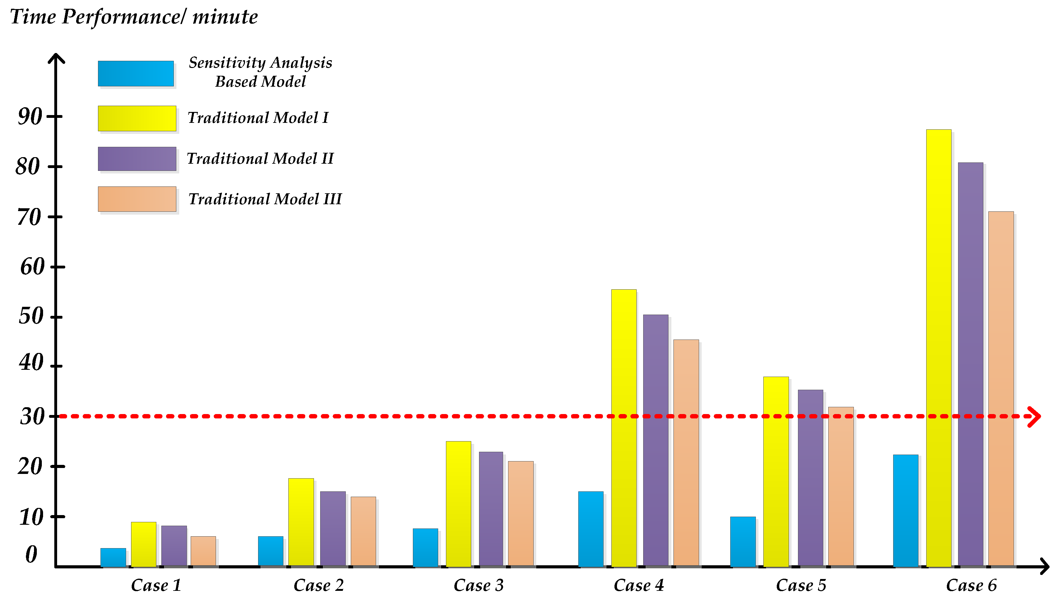
For all the over-load scenarios in Table 4, the load-shedding model based on sensitivity analysis and traditional load-shedding models are employed to verify the timeliness, respectively. In order to shorten the simulation time, the parallel computing modular in Matlab is employed [38,39,40]. Set the time limit of on-line power system operation risk assessment 30 min. The simulation results are portrayed in Figure 5.

In Figure 5, for case 1, 2, and 3, the three traditional load-shedding models can calculate them within 30 min because the amount of over-load scenarios is limited. With the increase of over-load scenarios, the calculating time of traditional models will be longer than 30 min such as case 4, 5 and 6, which cannot meet the requirements of timeliness in on-line power system operation risk assessment. Between the three traditional models, the time performance of model III is relatively better, which applies the direct power flow in optimal power calculation; model II is more efficient than model I because the nearby principle is applied, which can narrow the solution range. However, for the proposed load-shedding model in this manuscript, it can calculate all the 6 cases within 30 min. The reason of this circumstance is the target load bus has been dramatically reduced to some limited load bus by employing the sensitivity analysis. Thus, the time cost of calculating is saved, which brings about the improvement of calculation efficiency. When evaluating an actual power system with multiple nodes, the load-shedding model based on sensitivity analysis can be better applied in on-line operation risk assessment.

By comprehensively considering the importance of load bus and adjacency principle regarding the electrical coupling relationship, a load-shedding model is established to get the minimum value of the load reduction from different kinds of load buses, which is solved by the primal dual interior point method.

5. Conclusions

The traditional load-shedding models usually use global optimization to get the load-shedding range, which will cause multiple variables, huge computing scale and other problems. This makes it hard to meet the requirements of timeliness in on-line power system operation risk assessment. Thus, a load-shedding model based on sensitivity analysis is proposed in this manuscript, which can solve the existing problems of traditional load-shedding models. From our theoretical studies and simulation results the following conclusions may be drawn:

(1)

A novel filtration principle for confirming the load reduction region is proposed, which comprehensively takes the sensitivity of load bus on its input power and the sensitivity of over-load branch on each bus into consideration. In this way, global optimization is turned to local optimization, which can narrow the solution region and improve the filtration efficiency.

(2)

By comprehensively considering the importance of each load bus and adjacency principle regarding the electrical coupling relationship, a load-shedding model is established. The objective of the proposed load-shedding model is to achieve the minimum value of the load reduction from different kinds of load buses. The primal dual interior point method is applied to solve the established model.

(3)

Based on the IEEE 24-bus system, the proposed load-shedding model and traditional model are employed to calculate four different scenarios. The calculation results of the proposed model are equal to the traditional model. Besides that, the IEEE 300-bus and two other multi-node system are applied to testify the timeliness by comparing the calculation time of all the “N-1” and “N-2”over-load scenarios. For the multi-node system, the proposed model can dramatically reduce the calculation time. These simulation results testify the correctness and validity of the proposed load-shedding model.

References

- Mao, A.; Zhang, L.; Lv, Y.; Gao, J. Analysis on large-scale blackout occurred in South America and North Mexico interconnected power grid on Sep. 8, 2011 and lessons for electric power dispatching in China. Power Syst. Technol. 2012, 4, 74–78. [Google Scholar]
- Makarov, Y.V.; Reshetov, I.; Stroev, V.A.; Voropai, N.I. Blackout in North America and Europe: Analysis and generation. In Proceedings of the IEEE Russia Power Tech, St. Petersburg, Russia, 27–30 June 2005; pp. 1–7. [Google Scholar]
- Michael, A.; Robert, A.; Partrick, S.S.; Robert, S.; Mark, B. Critical operation power systems: Improving risk assessment in emergency facilities with reliability engineering. IEEE Ind. Appl. Mag. 2013, 5, 379–392. [Google Scholar]
- Chiris, J.D.; Janusz, W.B. Non-iterative method for modeling systematic data errors in power system risk assessment. IEEE Trans. Smart Grid. 2011, 26, 120–127. [Google Scholar]
- Liu, Y.; Zhou, J. The optimal load-shedding model in power system reliability assessment. J. Chongqing Univ. 2003, 10, 52–55. [Google Scholar]
- Zhao, Y.; Zhou, J.; Zhou, J.; Xie, K.; Liu, Y.; Kuang, J. A heuristic approach to local load shedding scheme for liability assessment of composite generation and transmission system. Power Syst. Technol. 2005, 23, 34–39. [Google Scholar]
- Liu, H.; Sun, Y.; Wang, P.; Cheng, L.; Goel, L. A novel state selection technique for power system reliability evaluation. Eletric Power Syst. Res. 2008, 6, 1019–1027. [Google Scholar] [CrossRef]
- Zhuo, Y.; Chen, C.; Wang, Z.; Liao, P.; Lin, X.; Xu, J. Research of acceleration algorithm in power system risk assessment based on scattered sampling and heuristic local load shedding. In Proceedings of the Annual IEEE System Conference, Orlando, FL, USA, 18–21 April 2016; pp. 1–5. [Google Scholar]
- Zhao, Y.; Zhou, J.; Liu, Y. ; Analysis on optimal load shedding model in reliability evaluation of composite and transmission system. Power Syst. Technol. 2004, 10, 34–37. [Google Scholar]
- Wang, P.; Ding, Y.; Goel, L. Reliability assessment of restructured power system using optimal load shedding technique. IET Gener. Transm. Distrib. 2009, 7, 628–640. [Google Scholar] [CrossRef]
- Rustam, V.; Sergey, G.; Valdislav, O. Mathematical models and optimal load shedding strategies for power system generation adequancy problem. In Proceedings of the 14th International Conference on Engineering of Modern Electric Systems, Oradea, Romania, 1–2 June 2017; pp. 41–46. [Google Scholar]
- Thelma, S.P.F.; Lenzi, J.R.; Miguel, A.K. Load shedding strategies using optimal load flow with relaxation of restrictions. IEEE Trans. Power Syst. 2008, 2, 712–718. [Google Scholar]
- Fu, X.; Wang, X. New approach to load-shedding in static state security analysis of power system. Proc. CSEE 2006, 9, 82–86. [Google Scholar]
- Dong, Z.; Miao, W.; Jia, H. Minimum load shedding calculation based on static voltage security region in load injection space. In Proceedings of the 2011 IEEE Region 10 Conference, Bali, Indonesia, 21–24 November 2011; pp. 959–963. [Google Scholar]
- Chen, G.; Wang, Y.; Lu, G.; Hu, J.; You, D.; Zhang, F.; He, Z. An improved load-shedding model based on power flow tracing. In Proceedings of the 12th World Congress on Intelligent Control and Automation, Guilin, China, 12–15 June 2016; pp. 1590–1593. [Google Scholar]
- Niu, R.; Zeng, Y.; Cheng, M.; Wang, X. Study on load-shedding model based on improved power flow tracing method in power system risk assessment. In Proceedings of the 2011 4th International Conference Utility Deregulation and Restructuring and Power Technologies, Weihai, Shangdong, China, 6–9 July 2011; pp. 45–50. [Google Scholar]
- Ren, J.; Li, S.; Yan, M.; Guo, Y. Emergency control strategy for line overload based on power flow tracing algorithm. Power Syst. Technol. 2013, 2, 392–397. [Google Scholar]
- Huang, H.; Li, F. Sensitivity analysis of load-damping characteristic in power system frequency regulation. IEEE Trans. Power Syst. 2013, 2, 1324–1335. [Google Scholar] [CrossRef]
- Adly, A.G.; Mathure, S. Application of active power sensitivity to frequency and voltage variations on load shedding. Electric Power Syst. Res. 2010, 3, 306–310. [Google Scholar]
- Yuan, J.; Duan, X.; He, Y.; Shi, D. Summarization of the sensitivity analysis method of voltage stability in power systems. Power Syst. Technol. 1997, 9, 7–10. [Google Scholar]
- Cai, X.; Wu, Z.; Kuang, W.; Fang, R.; Wang, L.; Li, K. Study on sensitivity of available transfer capability based on DC distribution factors. Power Syst. Technol. 2006, 18, 45–48. [Google Scholar]
- Di Fazio, A.R.; Russo, M.; Valeri, S.; de Santis, M. Sensitivity-based model of low voltage distribution systems with distributed energy resources. Energies 2016, 10, 801. [Google Scholar] [CrossRef]
- Li, C.; Yu, J.; Xie, K.; Zhang, Q. Model and algorithm of current tracing based on extended incident matrix. Trans. China Electrotech. Soc. 2008, 4, 104–111. [Google Scholar]
- Wu, Z.; Liu, D.; Zhou, H. Preventive control decision making based on risk analysis for power system security warning. Electric Power Autom. Equip. 2009, 9, 105–108. [Google Scholar]
- Yang, S.; Li, Y.; Hu, X.; Pan, R. Optimization study on k value of k-means algorithm. Theory Appl. Syst. Eng. 2006, 2, 97–101. [Google Scholar]
- Fan, Z.; Chang, X.; Wang, H.; Pu, T.; Yu, T.; Liu, G. Discrete reactive power optimization based on interior point filter algorithm and complementarity theory. In Proceedings of the 2014 International Conference on Power System Technology, Chengdu, China, 20–22 October 2014; pp. 210–214. [Google Scholar]
- Sanjay, K.P.; Sabha, R.A.; Rakesh, M.; Bhim, S. Interior point algorithm for optimal control of distribution static compensator under distorted supply voltage conditions. IET Gener. Transm. Distrib. 2016, 8, 1778–1791. [Google Scholar]
- Chen, Q.; Guo, R. A hybrid active power optimization algorithm based on improved genetic algorithm and primal-dual interior point algorithm. Power Syst. Technol. 2008, 24, 50–54. [Google Scholar]
- Yong, H.L.; Jin, H.J.; Gyeong, M.C. A new primal dual interior point algorithm for semi-definite optimization. In Proceedings of the 2014 International Conference on Information Science & Applications, Seoul, Korea, 6–9 May 2014; pp. 1–4. [Google Scholar]
- Yakowitz, S. The stagewise Kuhn-Tucker condition and differential dynamic programming. IEEE Trans. Autom. Contr. 1986, 31, 25–30. [Google Scholar] [CrossRef]
- Subcommittee, P.M. IEEE reliability test system. IEEE Trans. Power Appar. Syst. 1979, 6, 2047–2054. [Google Scholar] [CrossRef]
- Zimmerman, R.D.; Murillo-Sanchez, C.E.; Thomas, R.J. MATPOWER: Steady-state operations, planning and analysis tools for power systems research and education. IEEE Trans. Power Syst. 2011, 26, 12–19. [Google Scholar] [CrossRef]
- Murillo-Sanchez, C.E.; Zimmerman, R.D.; Anderson, C.L.; Thomas, R.J. Secure planning and operations with stochastic sources, energy storage and active demand. IEEE Trans. Smart Grid. 2013, 4, 2220–2229. [Google Scholar] [CrossRef]
- Palaniswamy, K.A.; Sharma, J.; Misra, K.B. Optimum load shedding taking into account of voltage and frequency characteristics of loads. IEEE Power Trans. Power Appar. Syst. 1985, 6, 1342–1348. [Google Scholar] [CrossRef]
- Wang, P.; Billington, R. Optimum load-shedding technique to reduce the total customer interruption cost in a distribution system. IEE Proc. Gener. Transm. Distrib. 2000, 147, 51–56. [Google Scholar] [CrossRef]
- Da Silva, A.M.L.; Cassula, A.M.; Billiton, R.; Manso, L.A.F. Optimum load shedding strategies in distribution systems. In Proceedings of the 2001 IEEE Porto Power Tech Proceedings, Porto, Portugal, 10–13 September 2001. [Google Scholar]
- Fliscounakis, S.; Panciatici, P.; Capitanescu, F.; Wehenkel, L. Contingency ranking with respect to overload in very large power systems taking into account uncertainty, preventive and corrective actions. IEEE Trans. Power Syst. 2013, 28, 4909–4917. [Google Scholar] [CrossRef]
- Yuan, S.; Huang, X.; Yang, X. Configuration and application of Matlab parallel computing cluster under windows environment. Comput. Mod. 2010, 5, 189–194. [Google Scholar]
- Ritesh, R.; Neeharika, K.; Nitiv, R. Digital image processing through parallel computing in single-core and multi-core systems using Matlab. In Proceedings of the 2017 2nd IEEE International Conference on Recent Trends in Electronics, Information & Communication Technology, Bangalore, India, 19–20 May 2017; pp. 462–465. [Google Scholar]
- Cao, J.; Fan, S.; Yang, X. SPMD performance analysis with parallel computing of Matlab. In Proceedings of the 2012 Fifth International Conference on Intelligent Networks and Intelligent Systems, Tianjin, China, 1–3 November 2012; pp. 80–83. [Google Scholar]
Figure 1.
The flow diagram of determining the load reduction region.
Figure 2.
The flow diagram of the load-shedding model based on sensitivity analysis.
Figure 3.
The structure diagram of the IEEE 24-bus system.
Figure 4.
Amount of load-shedding results of the IEEE 24-bus system (a) Scenario 1; (b) Scenario 2; (c) Scenario 3; (d) Scenario 4.
Figure 5.
Simulation results of time performance on three multi-node systems.