Methodology for Detecting Malfunctions and Evaluating the Maintenance Effectiveness in Wind Turbine Generator Bearings Using Generic versus Specific Models from SCADA Data

Abstract

This article offers reasons to defend the use of generic behavior models as opposed to specific models in applications to determine component degradation. The term generic models refers to models based on operating data from various units, whereas specific models are calculated using operating data taken from a single unit. Moreover, generic models, used in combination with a status indicator, show excellent capacity for detecting anomalies in the equipment and for evaluating the effectiveness of the maintenance actions, resulting in lower development and maintenance costs for the operating firm. Artificial neural networks and moving means were used to calculate the degradation indicators, based on the remainders in the model. The models were developed from operating data from fourteen wind turbines monitored over several years, and applied to the detection of faults in the bearings on the non-drive end of the generator. The use of generic models may not be recommendable for detecting faults in all cases, and the suitability will depend greatly on the context of the methodology developed to detect each type of fault, according to the element causing the fault and the fault mode, since each methodology requires a greater or lesser degree of precision in the model.

1. Introduction

We are currently experiencing a scenario of continuous growth in energy consumption on a global scale, leading to greater and progressively increasing demand which needs to be satisfied [1,2,3,4], while maintaining the quality and reliability of the system [5,6,7]. Energy generation from conventional sources, such as coal and oil contributes to an increase in pollution and global warming [8]. Of all forms of renewable energy, the one that has experienced most growth in recent years is wind power [9,10]. In order to ensure that this growth is not slowed, such facilities need to be made more attractive to investors.

The use of condition monitoring systems in the wind industry, as predictive maintenance systems onshore [11] and especially offshore [12], has clearly improved energy efficiency, reducing energy losses, and reduced the running costs of wind plants [13], with the consequent reduction of the impact of the failures and its maintenance costs thanks to reduction in logistic times, warehouse optimization, financial costs, etc. By using artificial intelligence techniques in maintenance, it is possible to identify failure patterns in equipment and thus anticipate possible failures [14,15,16,17] with the final purpose of increasing the life cycle of the wind turbines.

The principle of condition-based maintenance [18], considers that if it is possible to identify that a component is degraded and might fail within a given period of time, then preventative maintenance can be performed before that failure actually occurs. In the case of a wind turbine, that means increasing the energy produced, since the maintenance task can be performed at times when any energy that might be generated by the wind is negligible or non-existent. At the same time, it enables maintenance costs to be cut by preventing greater damage were the failure to actually occur.

Knowing what is going to fail makes it possible to optimize spare part management [19] and reduce the logistical waiting times involved in performing the maintenance task. Moreover, by using these techniques it is possible to extend the useful service life of the assets [20] according to the knowledge of the failure. Condition-based maintenance practice can be achieved based on three stages [21]: in a first stage the detection process identify anomalies in the behavior of the equipment [11]. Once it has been determined that the equipment is not working under normal conditions, it is necessary to identify the type of anomaly occurring in the machine [15,18,22,23,24], this second knowledge stage is named diagnostics. Finally, once the detection and diagnosis have been done, it is possible to estimate how the degradation of that specific failure mode will evolve and subsequently when the failure will probably happen (the third stage, prognosis) [22,25,26].

Failure modelling is an extremely complex science; very few data are typically available for failure incidents and, generally speaking, the appearance and development of the failures varies greatly. For that reason there are studies that seek to construct a physical model of the equipment and its control system to simulate failures in order to evaluate the behavior under failure conditions. These methods allow one to design robust fault tolerant control strategies for wind turbines. Most of these methodologies are supported by fuzzy logic and they are useful to train a diagnosis system and isolate the failure [27,28]. In this field, several studies were conducted: simulations of sensor failures and multiple failures were studied in [29,30]; an adaptive fuzzy system for fault tolerant control and cooperative control were applied to detect blade erosion and debris build-up in [31]; and two active power control schemes are developed based on adaptive pole placement control and fuzzy gain-scheduled proportional-integral control approaches in [32]. These studies represent the evolution to condition base operation, and knowing the real heath of equipment and isolating its failure one can adapt the control strategy to extend the remaining life of the equipment, as it was presented in [33].

Other techniques, that were used to evaluate the health of mechanical equipment, were introduced in [34], where the authors combined vibration analysis and normal behavior temperature model using artificial neural networks (ANNs). An ANN allows training a black box model without knowing the physical behavior of the equipment, which is extremely complex. The combination of SCADA systems, databases and ANNs are becoming popular in artificial intelligence development due to the fact a deep knowledge of the physical rules that are involved in the process is not needed.

Previous contributions have analyzed the use of SCADA data and ANN to create normal behavior models to detect malfunctions: an intelligent system for predictive maintenance applications to health condition monitoring in wind turbines was presented in [35]. They created normal behavior models and bounds, nevertheless they do not compare different model configurations to improve the goodness of fit the model, nor the utilization of generic models versus specific models. Each equipment is unique and a single model must therefore be generated for each one, based on its specific data [36]. However, data is not generally available for all units. When the unit is new, there will not be enough data to allow it to be modelled until a full year has passed, in order to have data for each season. This behavior model also varies and has to be recalculated whenever maintenance is carried out on the unit. On the other hand, in operational processes it is not desirable to wait for enough data to be available, it is easy to fall into the trap of using models built from limited historical data from a period of time with high failure risk due to premature damage. As a result, the model will be very imprecise and more susceptible to aberrant data in the sample, thus requiring more complex data processing. At the same time, making a separate model for each physical unit has a very high computing and expert labor cost.

In more recent studies, specific models to detect failures analyzing the residual values were used [37,38]. The use of generic models were introduced in [39]. The use of moving means of the residuals to detect bearing faults in wind turbines was included to this concept and the failure was considered when the moving mean of the residuals surpasses the fixed value of 2 °C, leading to the prediction of faults 1.5 h before their occurrence [40]. Moreover, it was decided to model the normal operating behavior of the machine using ANN techniques as it was done in [41,42]. That means to make a model of the behavior of the equipment based on a data set from a period when the unit has no failure [38,39].

The purpose of this article is to detect, with time enough to react, incipient failures or malfunctioning in the bearings on the non-drive end (NDE) of a generator using normal behavior models and evaluation over the lifetime of the degradation indicator. This article compares the goodness of fit of three normal behavior models: (i) firstly a Specific Model trained with a high volume of data from an unique wind turbine generator, (ii) secondly a Generic Model trained with operation data from several wind turbine generators with the same characteristics, but using a smaller historical data set from each wind turbine, and (iii) the third model is a variant of the Specific Model trained with a reduced data set after a generator bearing replacement (Specific Model After Correction). Moreover, Generic Models present less maintenance cost and offer fast development with fewer hardware and software requirements. This article also compares different ANN configurations to improve the goodness of fit of the models and shows a novel configuration of the normal behavior bound for a detection indicator.

The reminder of the paper is organized as follows: Section 2 involves analysis, selection and processing of the available operational data. In Section 3 the behavior of the temperature of the bearing is modelled using generic and specific models. Moreover, in Section 4 a status indicator is prepared to operate adequately with generic models. In Section 5, this indicator is used to show not only its capacity to detect degradation in the bearing but also its capacity to evaluate the maintenance operations. Finally, economic savings of implementing the model in some wind farms are shown in Section 6 and the conclusions are drawn in Section 7.

2. Parameter Description and Treatment

Both operational analogical [38,39] and digital alarms [43] registered from the SCADA can be used to evaluate the generator condition. Based on expert assessment and preliminary studies [38,44,45,46], the analogical operating variables of the wind turbines considered for creating the temperature model of the NDE bearing [47] in the generator are shown in

Table 1. Variables of the wind turbines considered for creating the temperature model of the NDE bearing (°C).

Variable	Units
Temperature of the drive-end (DE) bearing in the generator	°C
Generator voltage	kV
Temperature of slip rings	°C
Reactive capacity	kVA
Maximum temperature of the generator windings	°C
Power factor	-
Temperature inside the nacelle	°C
Stator active power	kW
Generator rotating speed	rpm
Rotor active power	kW
Wind speed	m/s
Total active power	kW

.

The sample consists of the training data set and the detection data set. On the one hand, the training data set is subdivided into two subgroups: the first one to train the neural networks (80%) and the second to calculate the equipment status indicators for a period of time in which the equipment does not present any faults (20%), which allows one to determine the “normal behavior” state of the equipment and its bounds. The packet used to train the neural net (the mentioned 80%) is divided into three sets: (i) 70% for training, (ii) 15% for testing and (iii) the other 15% for cross validation. On the other hand, the detection data set is used to validate the detection capacity of the indicators before the recorded failures.

From the training dataset, it is necessary to extract the data pertaining to periods in which the generator was malfunctioning. For this purpose, the data recorded from one month before a maintenance task or work order (WO) and the data from 12 h before a generator triggered alarm were removed. It is possible that some malfunction situations have not been eliminated from the sample. Given the large volume of data available to train the models, it was considered that these malfunction cases would not have a significant weight. A manual, statistical and multivariate filter was applied to the remaining training dataset. These data would be used to train the neural network corresponding to the temperature model for the NDE bearing and for calculating the status indicator in a period without failures. Both the statistical and the multivariable filter are only used in the data processing for training the models and configuring the normal operational range of the degradation indicator, but these filters are not used later in the monitoring process (detection dataset), due to the fact that if we filter aberrant data, we are removing precisely the kind of abnormal behaviors processes that we are trying to detect. The detection dataset was selected based on a period of time in which an order for replacement of the bearing was recorded, in order to check the indicator’s capacity for detection in dates prior to breakage of the bearing. These data are subject only to a manual filter.

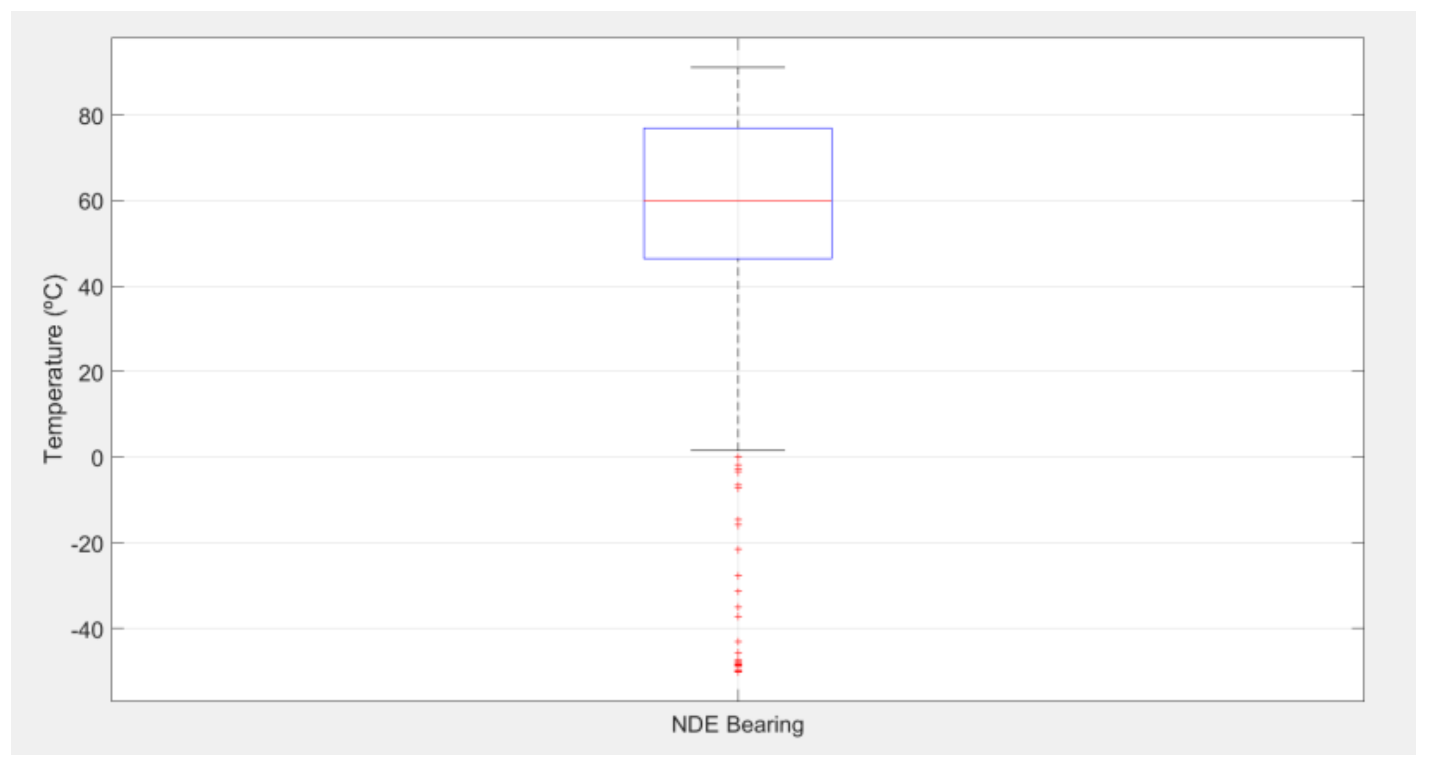
As a first step manual filtering is required, both for the training and validation datasets and the posterior detection dataset. For each of the variables under consideration, the manual filter only removes values that from the logical perspective of operation make no sense [38,40], possibly due to faults in the sensors or cases of clearly anomalous operation. Given that no limits of the operating variables are known, a statistical study was made using boxplot representations, as shown in Figure 1 for the temperature of the NDE bearing. Based on the values obtained the operating limits (lowest and highest) were obtained for each variable based on an expert judgement. It should be noted that because this filter is to be applied to the detection variables, it is very lax, with greater restrictions being applied in subsequent filters. 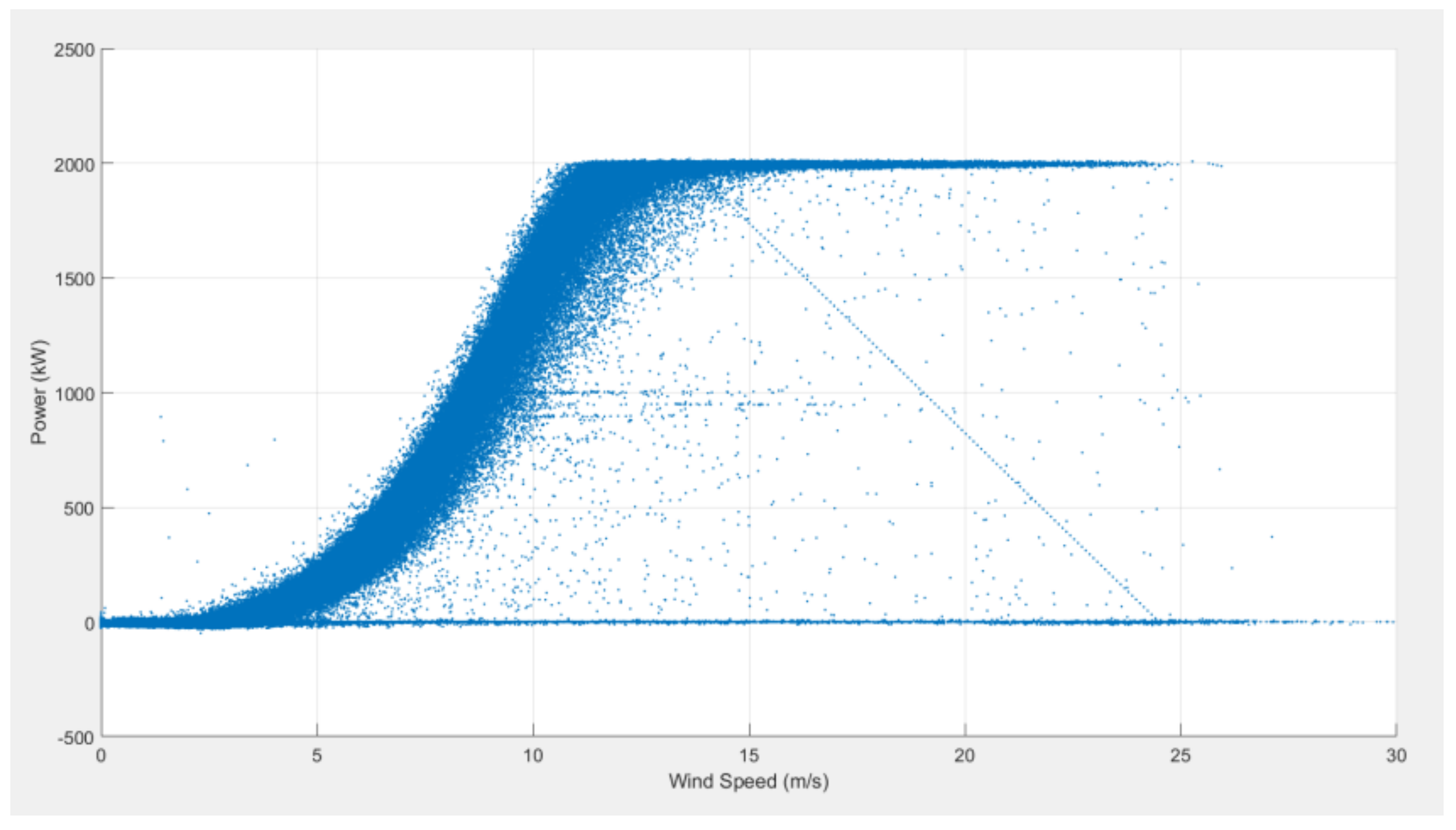Figure 2 is included as an example in which data on mean wind speeds of over 30 m/s have been removed.

The data normalization has a double purpose, prepare data for neural nets and identify those statistical aberrant data. The normalization has been carried out by subtracting the mean of the population set from each value and dividing it by the standard deviation, using the following expression:

$$i_{vNormalized}=\frac{i_v-\mu }{\sigma }$$

(1)

where µ is the mean and σ the standard deviation.

During the normalization process the statistical filter can be applied. This basically consists of eliminating any values that are more than three times the standard deviation. If a record is eliminated in the process of removing aberrant data, the data must be renormalized with the remaining sample. This process always is done almost once, but it may be repeated iteratively until there is no large number of data (10% of sampled data) more than three times the standard deviation, as in a normal distribution it would be expected to do that just once. During the process of normalizing the variables, the standardization parameters of each variable must be saved, since the input data for the model corresponding to the detection data must subsequently be normalized based on these parameters. The detection dataset therefore has to be normalized with µ and σ of the training dataset for the model to be applicable.

In statistical terms, aberrant data in a sample may be considered to be any whose value (normalized and absolute) is more than three times the standard deviation (σ). This criterion is applied when data distribution is normal. Not all operating variables match the criterion of normality, since the control systems restrict the operating values of the machine and act on the variables, forcing them to take non-normal values.

This statistical filter was applied to any variables that met the criterion of normality within the training and validation dataset. For this purpose the Shapiro–Wilk test can be performed, which is used to test the normality of a dataset. As a null hypothesis it is posited that a sample i₁, ..., i_n comes from a normally distributed population. This statistic is calculated using the following expression:

$$W=\frac{{({\sum }_{v=1}^n{a}_v{i}_{(v)})}^2}{{\sum }_{v=1}^n{(i_v-\mu )}^2}$$

(2)

where i_(v) is the number occupied by the vth position of the sample; µ is the mean of the sample and the variables a_n are calculated according to the expression:

$$\left(a_1,\dots ,a_n\right)=\frac{m^T{V}^{-1}}{\sqrt{\left(m^T{V}^{-1}{V}^{-1}m\right)}}$$

(3)

where m = (m₁, ..., m_n)^T, where m₁, ..., m_n are the mean values of the order statistic, of random independent variables, identically distributed, sampled from normal distributions. V is the covariance matrix of that order statistic.

The null hypothesis is rejected if W is too small. Where the hypothesis is null if p-value is less than the confidence level. In that case the data do not come from a normal distribution. Matlab has tools for performing these calculations quickly and simply in its Statistical Toolbox [41,48]. A function was then generated that applied the statistical filter to the data, only when the hypothesis is fulfilled.

The sample covariance used as a statistically estimated value of the parameter is:

$$C(i,j)=\frac{{\sum }_{v=1}^n(i_v-\overline{i})(j_v-\overline{j})}{n}$$

(4)

where C(i,i) and C(j,j) coincide with the typical deviation (σ) of i and of j.

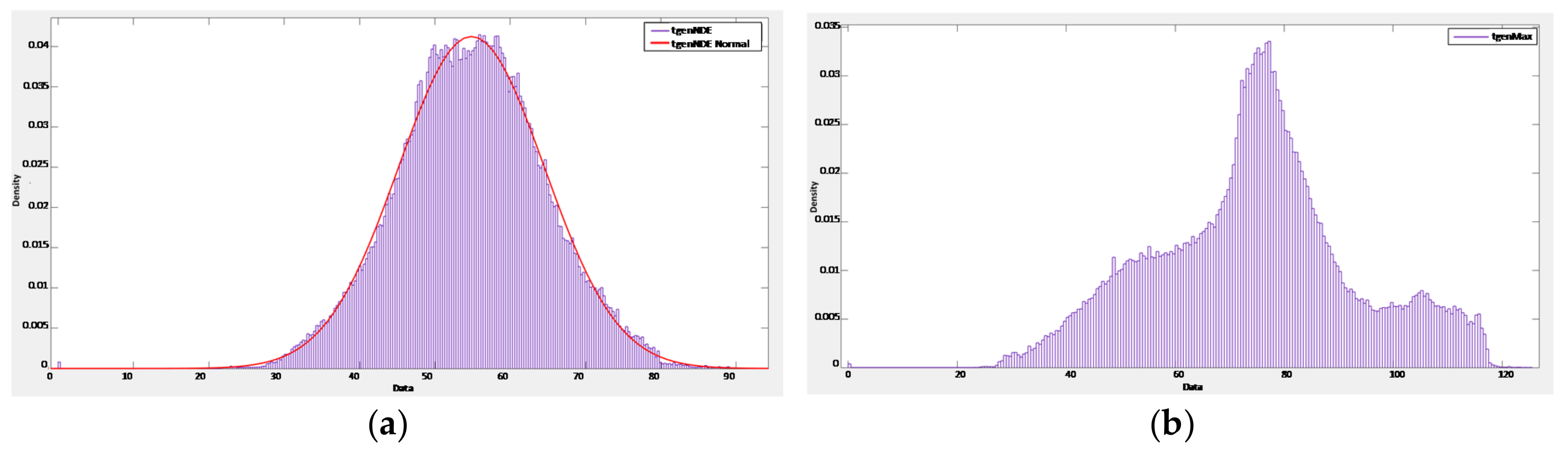
The NDE bearing temperature variable fulfils the condition of normality (Figure 3a). However, the maximum windings temperature variable did not fulfil the condition of normality (Figure 3b).

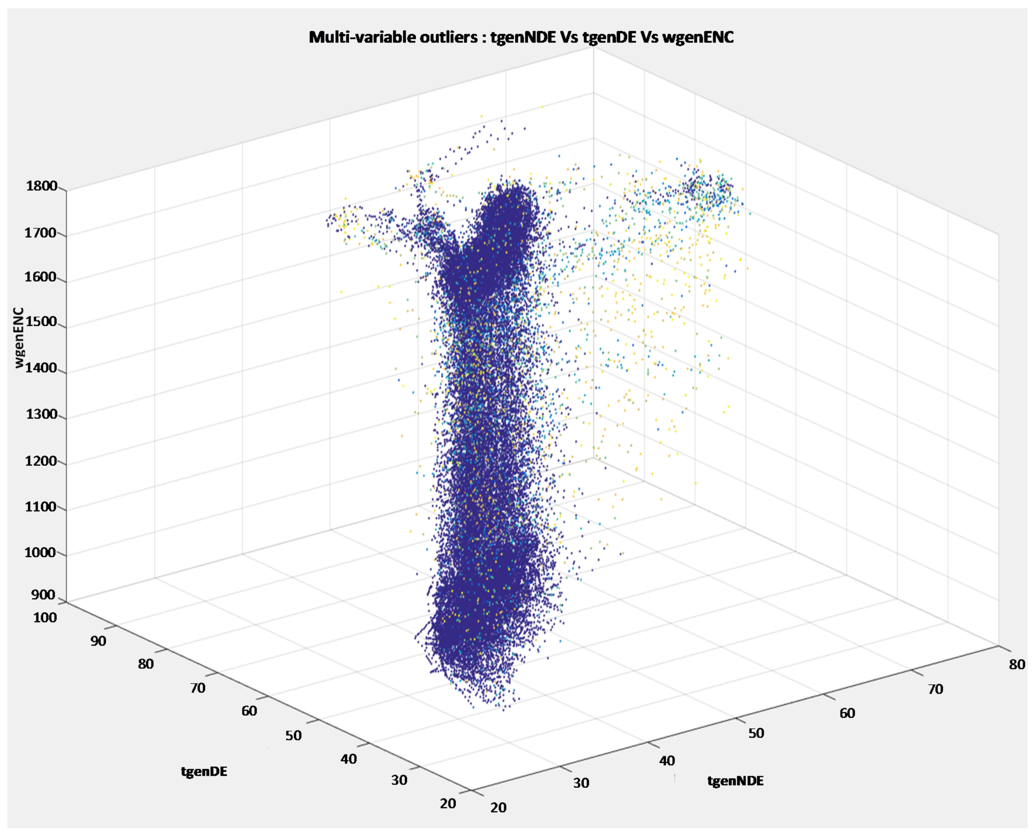
In order to identify atypical data in relation to other variables a multivariate filter was performed by applying cluster techniques [16]. Using hierarchical cluster techniques, a function was generated that identified the main block and the remaining adjoining clusters could be considered as outliers or aberrant. The method calculates the Euclidean distance between the different points for each of their variables and groups them according to these distances. The Euclidean distance between two points in the n-dimensional space (P = (p₁, p₂, ..., p_n) and Q = (q₁, q₂, ..., q_n)) is calculated as:

$$d=\sqrt{{\left(p_1-q_1\right)}^2+{\left(p_2-q_2\right)}^2+\dots +{\left(p_n-q_n\right)}^2}=\sqrt{{\displaystyle \sum }_{i=1}^n{\left(p_i-q_i\right)}^2}$$

(5)

The input parameter that varied in the tests was the number of groups to be made. If the number of groups is high, there is a risk that the algorithm will divide the main group into various sub-groups, corresponding to the different regions of operation. In other words, instead of detecting aberrant data, the data would be classified into different operating regions. If there are many scattered data, many groups will be formed with a unique datum and there will probably be aberrant data left unremoved. An optimal response needs to be found and this is a process that must not be performed automatically. After several tests, we decided fix the number of clusters as the 5% of the number of samples. Figure 4 shows how aberrant data are determined using multivariate techniques.

3. Normal Behavior Model Development

The main advantage of models with neural networks lies in the fact that it is not necessary to know the nature of the dataset to be represented; rather the neural network itself, through the training process, gathers the essential characteristics of the dataset to be represented [49]. This statement is true to a certain extent. For continuous processes in which there are no changes in the operating parameters (boundary conditions) it holds true. However, when the operating conditions vary depending on the control system of the wind turbines it is necessary to identify these regions and apply one or more neural networks for the modelling. Other advantages may be mentioned that the nonlinear behavior of the functions of activation of the neurons will enable the neural networks to act as universal approximators of nonlinear functions without depending on the knowledge of the experts on the modeled process [50]. Besides they can be adapted to the development of any type of data representation by just retraining them. This makes it possible to develop evolutionary models in such a way that one can have a set of networks that represent the original behavior of the unit and other networks that represent the present behavior of the unit [51]. The former are used to determine the degradation of a component (the case presented here) and the latter to determine faults that do not display any prior degradation [44]. On the other hand, neural nets require a large quantity of data for training neural networks with many inputs. In addition, exist the possibility of lead to some local minimum in the training process.

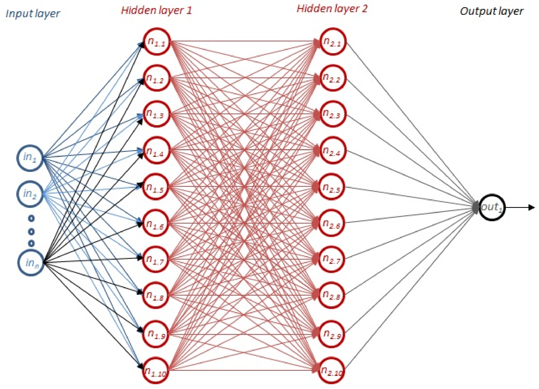
In order to create the NDE bearing temperature behavior model, a neural network of multilayer perceptron (MLP) type was used. This is a type of one-way neural network in which the neurons are organized in layers, so that the input of a neuron located in an intermediary layer can only be the output of the preceding layer, while its output serves as the input for neurons in the next layer. This is shown in Figure 5 and is adapted to our designed model: the blue neurons form the input layer, where each neuron from the input layer corresponds to the 12 operating variables selected; the red neurons form an intermediary or hidden layer, where a structure of two hidden layers with 10 neurons per layer was used in the developments; and black neurons form the output layer, where the output value is the NDE bearing temperature.

A MLP neural network can have various hidden layers, although with a single hidden layer, it would be capable of approximating, with an arbitrarily small error, any bounded continuous function (linear or non-linear), and with two hidden layers it could approximate any continuous function. Designing a MLP neural network involves selecting the number of hidden layers and the number of neurons in each layer. The greater the number of layers and neurons, the greater will be the capacity of the MLP neural network to fit any function, but it will increase the time required to train it (i.e., for it to perform learning), and, in particular, there is a risk of overtraining the network.

There are different learning and training techniques for MLP neural networks. In the same way as other authors [52], in this study the error backpropagation technique was used. The current temperature of the NDE bearing depends not only on the current values of the other variables, but also on the previous values, given the thermal inertia. For this reason, a time-delay variant of the MLP networks was used. This type of network is known as a focused Time Delay Neural Network (TDNN) [53,54]. 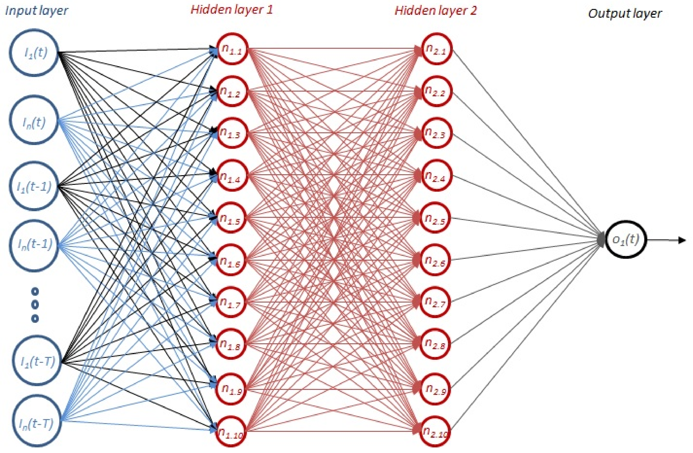Figure 6 shows a model of focused TDNN. In our case, there are 12 × 3 input neurons in the input layer (in blue), two hidden layers with 10 neurons each (in red), and an output layer (in black). However, the specific feature of the focused TDNN is that the input layer has several more neurons than the inputs of the neural network: the number of neurons in the input layer is a multiple of the inputs of the network and the number of time delays. Our neural network with 12 variables and three delays has 36 neurons in the input layer. The first group of twelve neurons takes the value of the inputs of the network in the instant t. The second group of twelve neurons of the input layer store the previous value (t − 1) of the input vector of the neural network (those three neurons are joined through time delay units, designated by z⁻¹, to the twelve neurons that take the value of the input vector of the neural network). The third group of twelve neurons stores the prior values of the neurons in the second group (therefore, the value of the input vector of the neural network with a delay of two time units, the t − 2 value). Thus, this TDNN, and in general all time delayed neural networks, has a structure that makes it possible to allows it to retain a memory of the activity of the neurons in the network with prior values from the input vector. A focused TDNN, with k units of delay and two inputs x₁(t) and x₂(t) is equivalent to an MLP neural network with the inputs:

$$x_1\left(t\right),x_2\left(t\right),x_1\left(t-1\right),x_2\left(t-1\right),x_1\left(t-2\right),x_2\left(t-2\right),\dots ,x_1\left(t-k\right),x_2\left(t-k\right)$$

(6)

As suggested in [11], the internal structure of the net is determined by trial-and-error to find the right number of hidden layers, neurons and training algorithms [55].

Using the created models, the NDE bearing temperature is estimated based on the input variables described in Table 1. The data used corresponds to real time data taken at ten-minute intervals (the 10-min means were not taken). When some datum was not available, the time record was preserved with NaN values (in Matlab NaN can be used for missing of no valid data), due to time delay neural networks were being used, it was necessary to preserve the complete timeline. In records in which some datum is missing, the neural network will not provide an estimate of the output; this was taken into account when calculating the status indicator. The fact of using a time delay in input values means that the data used to train, validate and calculate the subsequent indicator are not selected at random and the blocks are divided into consecutive time sequences.

3.1. Performance Analysis

Malfunctioning is detected from study of the development of the remainders between the model and the real value of the variable [16,18,38,39,40]. For each of the three models created several errors were calculated, namely:

Mean error (ME):

$$\mathrm{ME}=\frac{{\sum }_{i=1}^n(TRea{l}_i-TMode{l}_i)}{n}$$

(7)

Mean absolute error (MAE):

$$\mathrm{MAE}=\frac{{\sum }_{i=1}^n\left|TRea{l}_i-TMode{l}_i\right|}{n}$$

(8)

Mean square error (MSE):

$$\mathrm{MSE}=\frac{{\sum }_{i=1}^n{\left(TRea{l}_i-TMode{l}_i\right)}^2}{n}$$

(9)

Mean deviation or root mean square error (RMSE):

$$\mathrm{RMSE}=\sqrt{MSE}$$

(10)

Mean positive error (PE): similar to the ME but only takes into account those positive errors and ignores the negative ones. Percentage errors are calculated by dividing every nth error by the real value of the temperature:

Mean relative error (MRE):

$$\mathrm{MRE}=\frac{{\sum }_{i=1}^n\frac{(TRea{l}_i-TMode{l}_i)}{TRea{l}_i}}{n}$$

(11)

Mean absolute relative error (MARE or MAPE):

$$\mathrm{MARE}=\frac{{\sum }_{i=1}^n\left|\frac{TRea{l}_i-TMode{l}_i}{TRea{l}_i}\right|}{n}$$

(12)

Mean relative positive error (MRPE): similar to MRE but only takes into account those positive errors and ignores the negative ones. TReal_i is the real temperature measured in the NDE bearing (°C), TModel_i is the temperature estimated by the neural networks model developed (°C) and n is the total size of the sample

Based on these errors the precision of each of the models was evaluated, although it was accompanied with a visual inspection of the response of the models.

3.2. Prediction Model Selection

In order to generate the Specific Model, data corresponding to 2-year operating history of the wind turbine A01 were used, coinciding with a period in which it did not show any malfunctions. This model will only be applicable to estimate the signal of this same wind turbine. The Generic Model was calculated based on one-year operating data from the wind turbines A02 to A14 from within the same wind farm. This model will be applicable to any wind turbine with similar characteristics. To validate its goodness of fit the model simulation was applied on the wind turbine A01, using a data that were not used in the realization of the model. Finally, to obtain the Specific Model After Correction, as with the Specific Model, only a 2-month data set from the wind turbine A01, selected immediately after the bearing replacement, were used. In all cases, for validation and indicators configuration, the data were divided according to Section 2. For the comparison of errors between models, the same dataset were used, corresponding to the period after the dataset used train the Specific Model After Correction.

In order to define an optimal neural network structure for a productive environment, in a first approach experiments were carried out looking for a compromise between the error level of the model and the computational resources used. The comparison of several Specific Models was carried out, maintaining the same number of input variables and with a data set of a single wind turbine (A01) with an MLP network. The model was trained with the first two years of the equipment’s operation history and the error was calculated using the last year of operation. In this experiment the results were compared by varying the number of layers of hidden neurons from 1 to 3 and maintaining the number of neurons per layer in 10. Subsequently the number of neurons per layer was increased up to 20. Although the results obtained with this last configuration improve those obtained with two layers and 10 neurons per layer, the additional time necessary to train the model does not make this configuration advisable for a productive environment, since the time that needed was four times higher (

Table 2. Results obtained for the experiments by specific model net configuration.

	MLP				MLP Cascade		TDNN
Layers × Neurons per layer	1 × 10	2 × 10	3 × 10	2 × 20	2 × 10 (Cascade)		2 × 10 with no delay (MLP)	2 × 10 with 3 delays
Training algorithm	Levenberg-Marquardt	Levenberg-Marquardt	Levenberg-Marquardt	Levenberg-Marquardt	Bayesian	Levenberg-Marquardt	Levenberg-Marquardt	Levenberg-Marquardt
R	0.986	0.988	0.988	0.98995	0.9892	0.988	0.988	0.989
ME	0.01	0.02	0.02	−0.01	−0.01	0.02	0.02	−0.16
MAE	1.23	1.20	1.16	1.10	1.13	1.20	1.20	0.99
MSE	2.78	2.54	2.48	2.08	2.23	2.54	2.54	2.98
RMSE	1.67	1.59	1.58	1.44	1.49	1.59	1.59	1.73
PE	1.23	1.20	1.17	1.08	1.12	1.20	1.20	0.97

).

Subsequently, in a second experiment several training algorithms were tested, highlighting the Bayesian and Levenberg-Marquardt algorithms [56]. Firstly, a MLP network with two hidden layers and 10 neurons per layer was constructed, but a cascade neuron connection and training with the Bayesian algorithm. The training of the network required more than 12 h of calculation than in previous experiments and the results were not sensitively better than in other models, then the use of this training algorithm was discarded. Further testing was done with the cascade configuration but with the Levenberg-Marquardt algorithm and the results were similar to the standard feedforward connection, with the only improvement in training times that were reduced slightly with the cascade configuration.

In a third experiment, a TDNN network configuration was tested configuring the network with two hidden layers and 10 neurons per layer. The delay implies that in order to estimate the temperature at time t, at the input of the network the variables of time t, t − 1 and t − 2 are used. The results obtained without considering delay in the input versus considering 3 delays are shown in the Table 2, revealing that this last configuration is the one that presented better results. The objective variable in previous iterations was considered as input to estimate de current output value in [35], nevertheless in our study the objective variable is never considered as input. If the equipment is presenting over temperatures because of a failure, the model will estimate higher temperatures, being the failure hidden to detection.

Based on results in Table 2 it is verified that the model generated by the TDNN network reduces the error MAE and PE, which are the ones that were chosen as main reference to evaluate the performance of the models. However, the improvement does not justify the increase of computational resources necessary for the use of TDNN networks that multiply the number of inputs, and following the premise of defining the best methodology for a real production environment, from now on we will work with networks MLP.

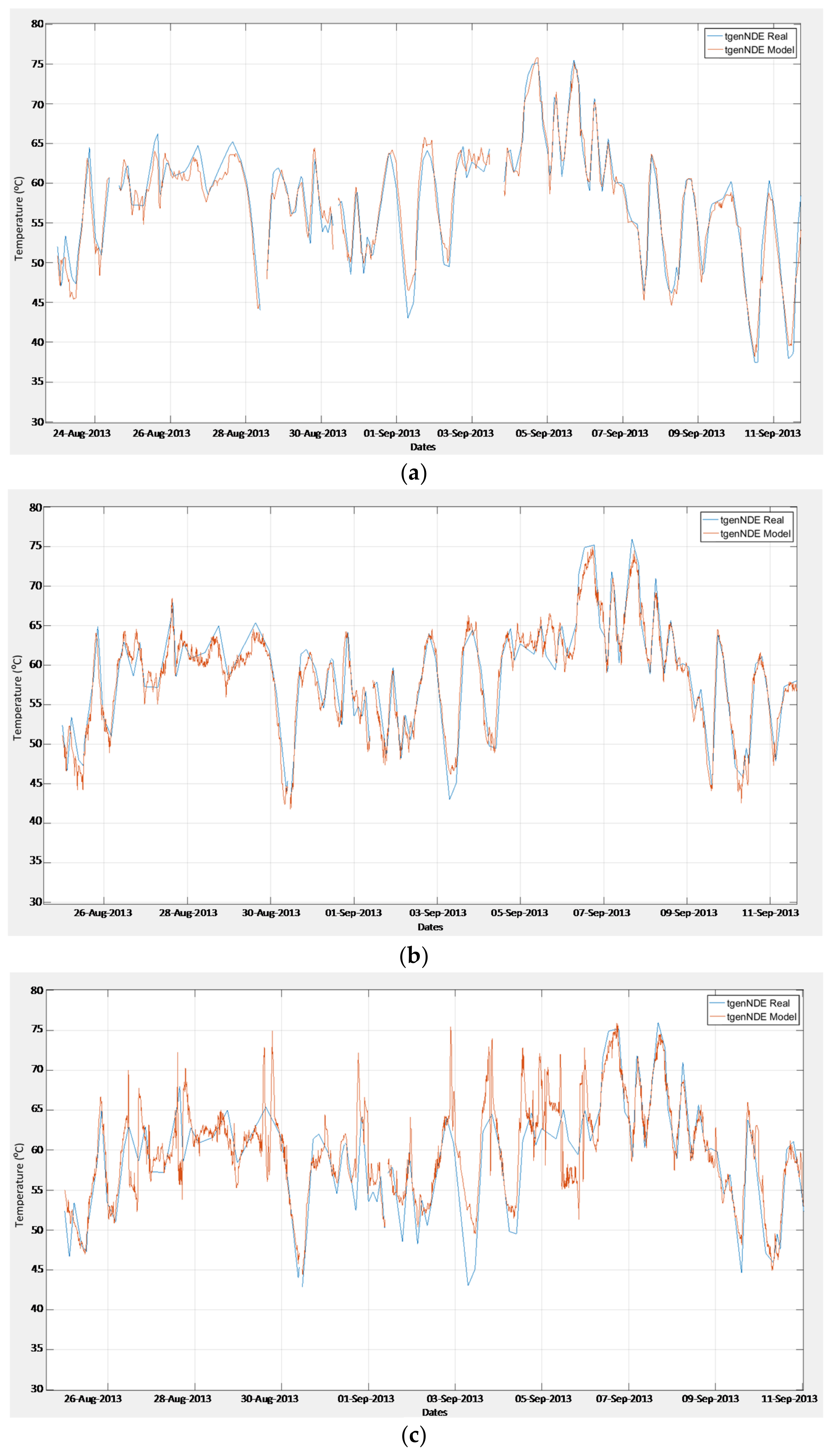
The Specific Model was developed using an approximately 105,120 time records of operating data. The errors obtained with the validation dataset are summarized in

Table 3. Errors obtained in the different models developed.

	Specific Model	Generic Model	Specific Model After Correction
Experiment	72	97	98
R	0.988	0.968	0.935
ME	0.02	0.12	0.36
MAE	1.20	1.33	2.27
MSE	2.54	3.21	10.21
RMSE	1.59	1.79	3.20
PE	1.2	1.36	2.44
MRE	0%	0%	0%
MARE	2%	3%	4%
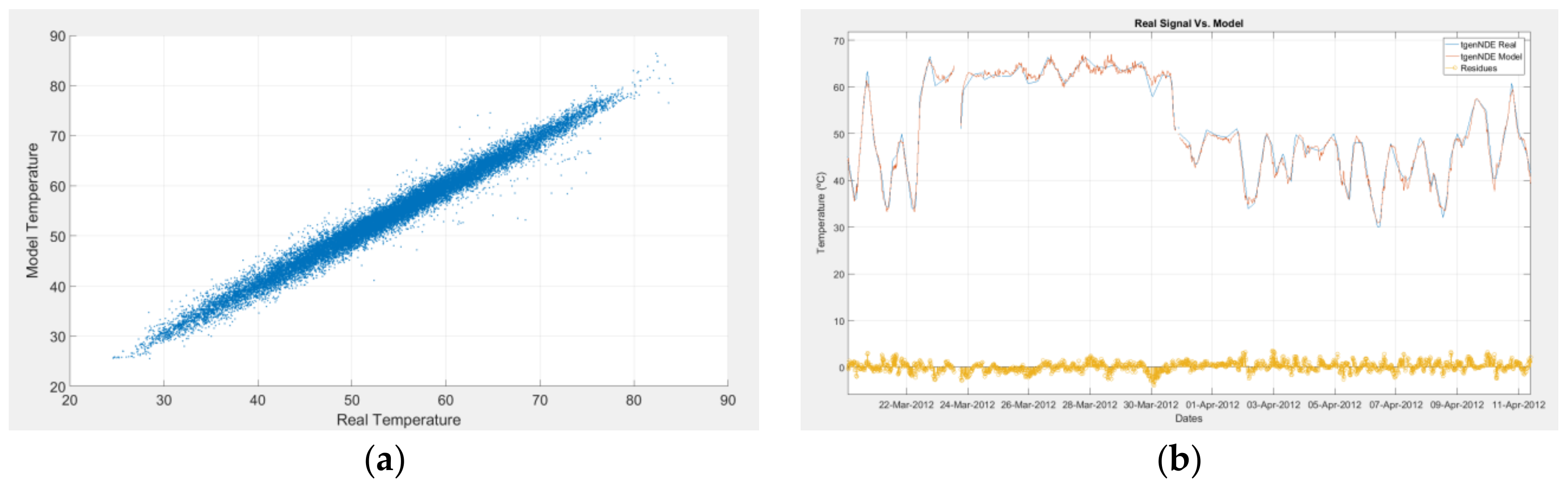
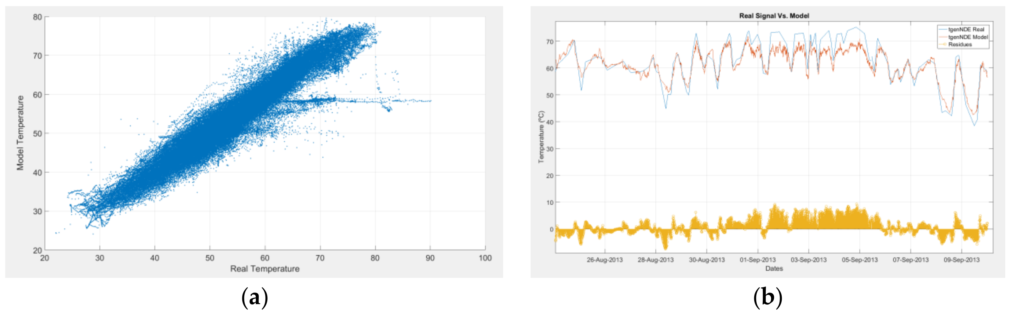
MRPE	2%	3%	4%

. By representing the regression line of the model, R = 0.988, the model can be seen to be very good, achieving linear and unscattered distribution. To compare the goodness of fit of the models it was preferred to use MAE and the RMSE. This was because the ME can prove confusing, since it is possible to have a very low mean error but a very high scattering of the model above and below certain points as it is shown in Figure 7a. Figure 7b shows the real temperature of the NDE bearing in blue and the temperature estimated by the model in red. At the bottom the remainders of the model are shown in yellow, and these are the ones subsequently used to calculate the indicator.

The Generic Model was trained with approximately 683,280 time records. This model is valid for generators from the same manufacturer and of the same model, and provided that they are operating under similar operating conditions (100% of time under running conditions and 100% data quality without communication losses). The model was developed using a large number of operating data from 13 generators with the same type of unit during a period without faults. 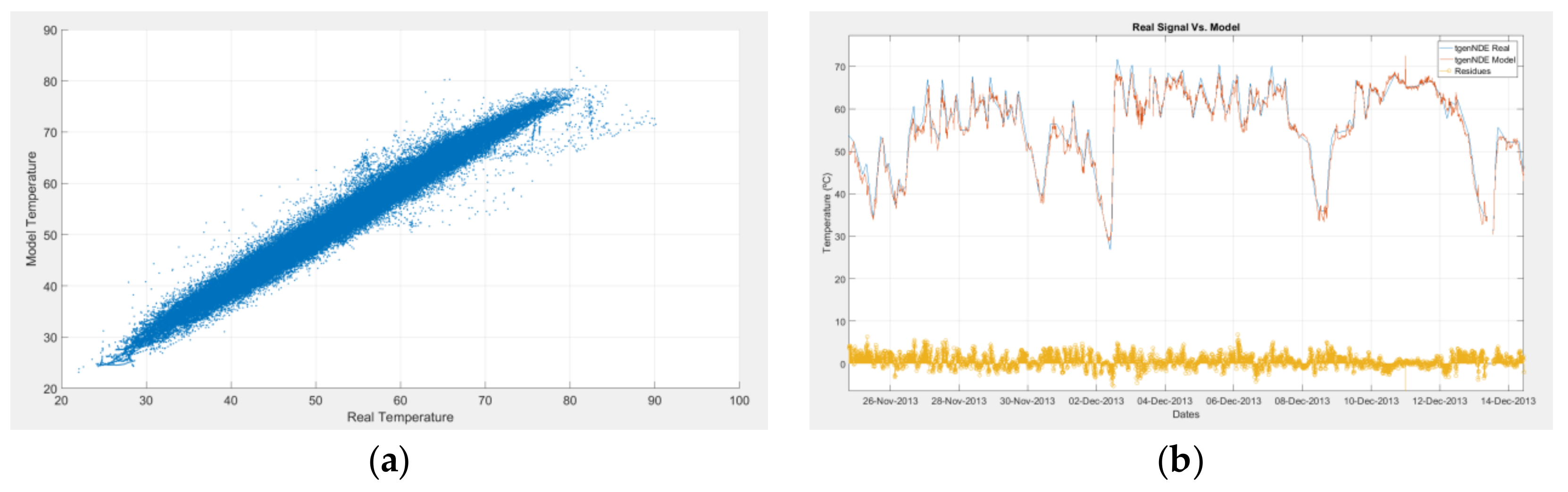The errors obtained with the validation dataset are summarized in Table 3. By representing the regression line of the model, R = 0.968, it can be seen that as in the previous case the model is very good, achieving a linear distribution that is somewhat more scattered than in the Specific Model. This is to be expected, given that although the behavior of the generators is similar, each unit has its own particularities, hence the scattering of values. Nonetheless, the difference in the errors calculated is negligible as it is shown in Figure 8a. As it can be seen from the regression line, some of the data used for validation of this model corresponded to values with a possible state of malfunctioning, since the real temperature is higher than that estimated by the model (Figure 8a). The fitness of the model can also be seen to be still very good, although it has greater variation than the Specific Model (Figure 8b).

The Specific Model After Correction was developed using approximately 8640 time records of operating data. The errors obtained with the validation dataset are summarized in Table 3. The MAE error has practically doubled. It would be necessary to have at least one year of new data following repair of the unit to have a representative model of the behavior of the temperature of the bearing. In Figure 9a it can be seen that the regression line is still more open than in the Generic Model and that one dataset remains horizontal, i.e., the real temperature rises, but the temperature according to the model remains constant. It is possible that the operator restricted the generator’s capacity—and thus also its temperature—following repair, with the result that the model has interpreted these data as being from correct operation and made a bad fit, in such a way that when similar operating conditions occurred, the model interpreted that the machine was again operating under the same conditions. Generally, it is necessary to let some time pass after a repair before any modifications settle down and everything is properly assembled, lubricated and tested. It would be particularly useful to develop complex models formed from expert systems that determine the operating situation of the wind turbine and apply different models. Figure 9b shows how the remainders are greater than in the previous models. The model is showing a defective fit mainly at high temperatures, possibly when the generator is operating at rated capacity or in a warmer period of the year. Given that the model is made with data for the winter months, the external temperature is lower and as we have seen in other studies [57], the temperature of the bearing depends on the time of year and the time of day and not only on the external temperature.

Figure 10a–c compare the difference in fluctuations in the response of the different models. Generic Model involves less precision, mainly because of its fluctuations, but the fit is excellent for developing a failure detection indicator. Other application would require models with a better accuracy due to the criticality of the process. We prefer to consider that the real situation of the data available is what it is; there are no perfect data and no perfect models. This means that instead of adapting the reality (data) to the methodology, we should adapt the methodology to the reality of everyday professional practice (i.e., the real data).

Although the specific models present a smaller error in the estimation of the signal, it has been demonstrated that the models that need to be updated after the repair are much less accurate than the generic models. In that way, an operator with an installed capacity of 18 GW could have 9000 wind turbines, with five main components per unit, with, for example, 10 critical points of status monitoring per unit. This would require creating and maintaining 450,000 behavior models based on neural networks. This is clearly inviable, since the work of analyzing and cleansing the data, training the models and continuous supervision and re-training (in the case of specific models) would require a very large number of expert workers and very powerful computing centers, not only to train the models, but to carry out monitoring and continuous estimation of the operating status of the units. This probe that it is not necessary to obtain more precise models for estimating the bearing temperature. Due to this fact we decided to continue using the Generic Model and to dismiss the Specific Model.

4. Failure Detection Indicator Configuration and Abnormal Level Quantification

The failure detection indicator proposed is based on calculation of the moving mean of the error presented by the model as compared to the real situation [11,18,40]. The behavior model used was the Generic Model, because it is valid for detecting degradation with the required precision.

Generic models can be applied indiscriminately to each wind turbine with the same type of equipment, taking into account that the anticipated error will be higher than that of a specific model for a single unit, and different in each wind turbine. Bigger residues do not affect to the calculation of the status indicators of the units, since such indicators are based on the evolution over time of the mean error between the model and reality. For example, if the model in a wind turbine has a mean error in temperature estimation of 5%, this error can be expected to remain constant until a degradation occurs, while if the error for another wind turbine were 10%, the same concept of detection would apply equally. In effect, the unit fails when the error between the model and the reality increases; mathematically, therefore, it is equivalent to introducing a different offset for each wind turbine between the model and the unit. This offset is calculated on the basis of data on operation without failure of each unit.

If the value of the indicator is calculated using a dataset in which the equipment has not shown malfunctioning or degradation, the mean error can be expected to remain constant. The indicator can therefore be expected to remain within certain intervals of variation. However, when a unit is degraded, its behavior will increasingly vary from that of the model. The remainders may therefore be expected to be ever greater and the mean value of the error will therefore be greater.

A moving mean model is one in which the value of the variable for an instant t is a function of an independent term and of a weighted succession of errors corresponding to the preceding instants. After several experiments and tests of response of the indicator, it was decided that the weighting of all prior errors should be the unit, i.e., the same weight was given to the error of instant t as to the error of instant t−T, where T is the moving window of calculation of the mean error.

In this way, the status indicator (Ind) is built:

$$Ind=\frac{{\sum }_{n=t-T}^{t}Error\left(n\right)}{T}$$

(13)

$$Error\left(n\right)=TRea{l}_i-TMode{l}_i$$

(14)

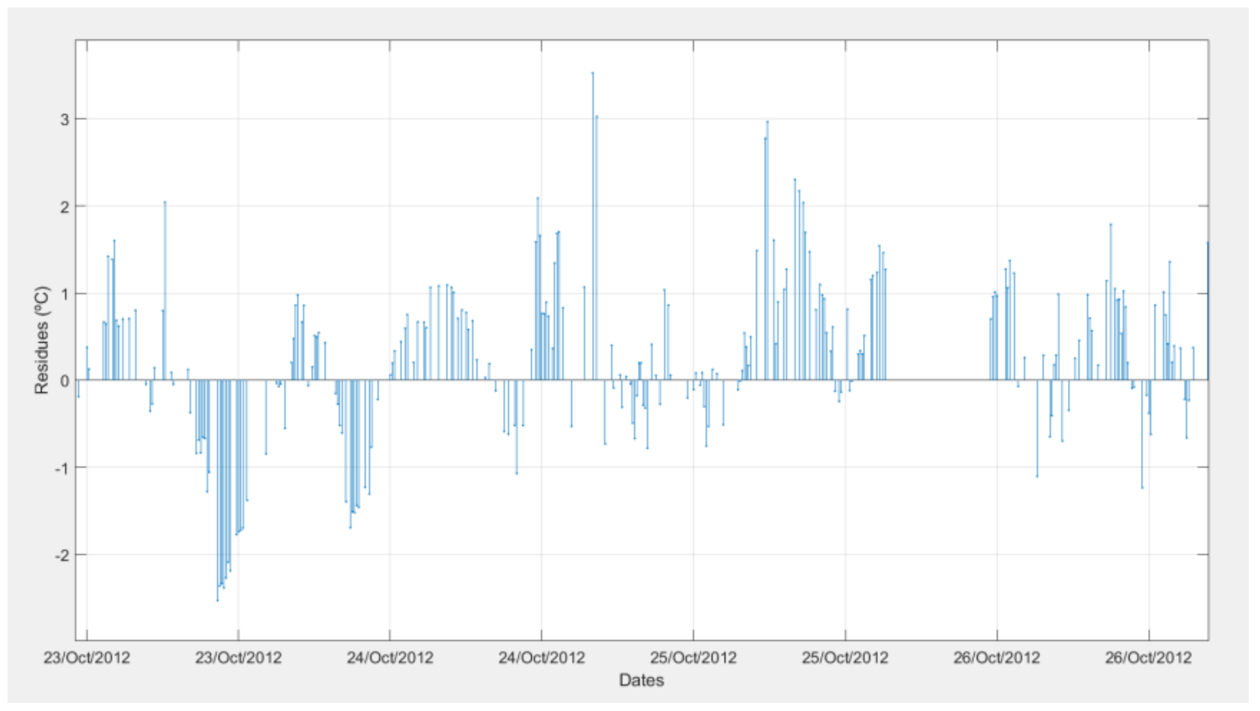
Based on the remainders shown in Figure 11, their moving mean is defined by adjusting the value T. The configuration of T cannot be decided on lightly, since the indicator will present one response or another accordingly.

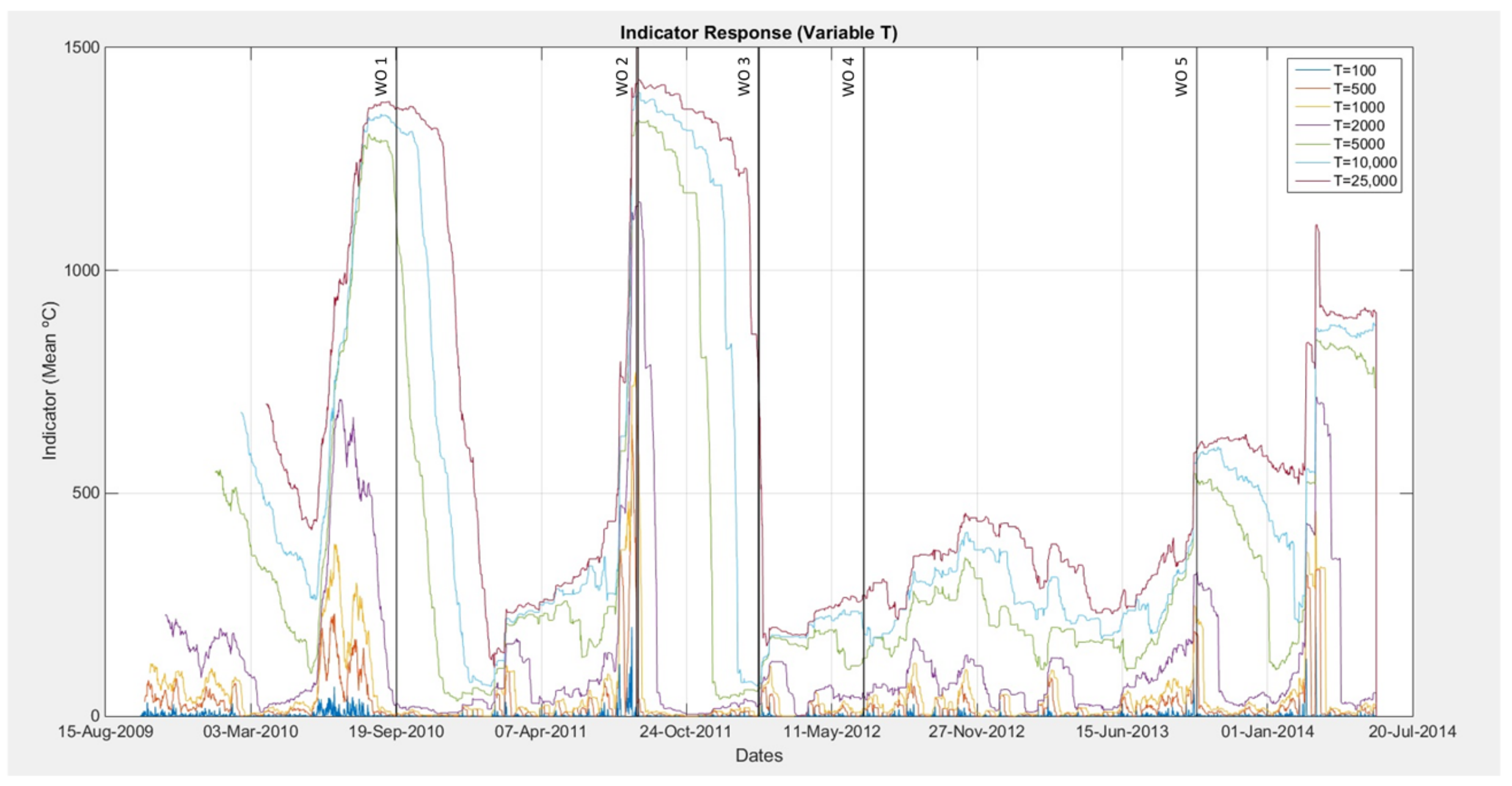
In the example shown in Figure 12, iterations of between 100 and 25,000 data were made, thus varying the period of calculation of the moving mean (T); values of T = 1000 data are equivalent to 1 week of 10-min data. Therefore, windows of time of between approximately 1 and 170 days were analyzed. With very short time windows (T = 100), indicators with a lot of noise are generated. In these cases, the value of the indicator varies greatly, and it is complicated to extract a clear trend from them. Using indicators of this type there is a risk of generating many false positives in detecting false malfunctions. The vertical lines show maintenance operations performed on the generator, some of which correspond to inspections or preventive maintenance and the indicator can therefore be expected not react to these operations. On the other hand, the indicator has reacted to failures in the generator (not inspections or preventive maintenance), but this should stabilize and return to values close to zero following the repairs, which does not occur when the windows of calculation of the moving mean are very high. Following a visual exploration of the reaction of the indicator before and after the faults it was concluded that the period of calculation T would be of 1000 10-min data. Once the indicator had been configured, the normal operating values were calculated, where normality was understood to be a lack of degradation or malfunctioning of the equipment.

By calculating the indicator with a dataset in the absence of faults, it was possible to determine the expected normality value of the indicator and its fluctuation intervals, the maximum and minimum values between which the equipment can be found to continue behaving as in the model. Given that the calculation period of the moving mean T is one week, this model does not serve to detect sudden failures, since large deviations would not show up immediately in the mean. This indicator is therefore valid for determining degradations that extend over time and which generally cannot be detected by the operating SCADA. 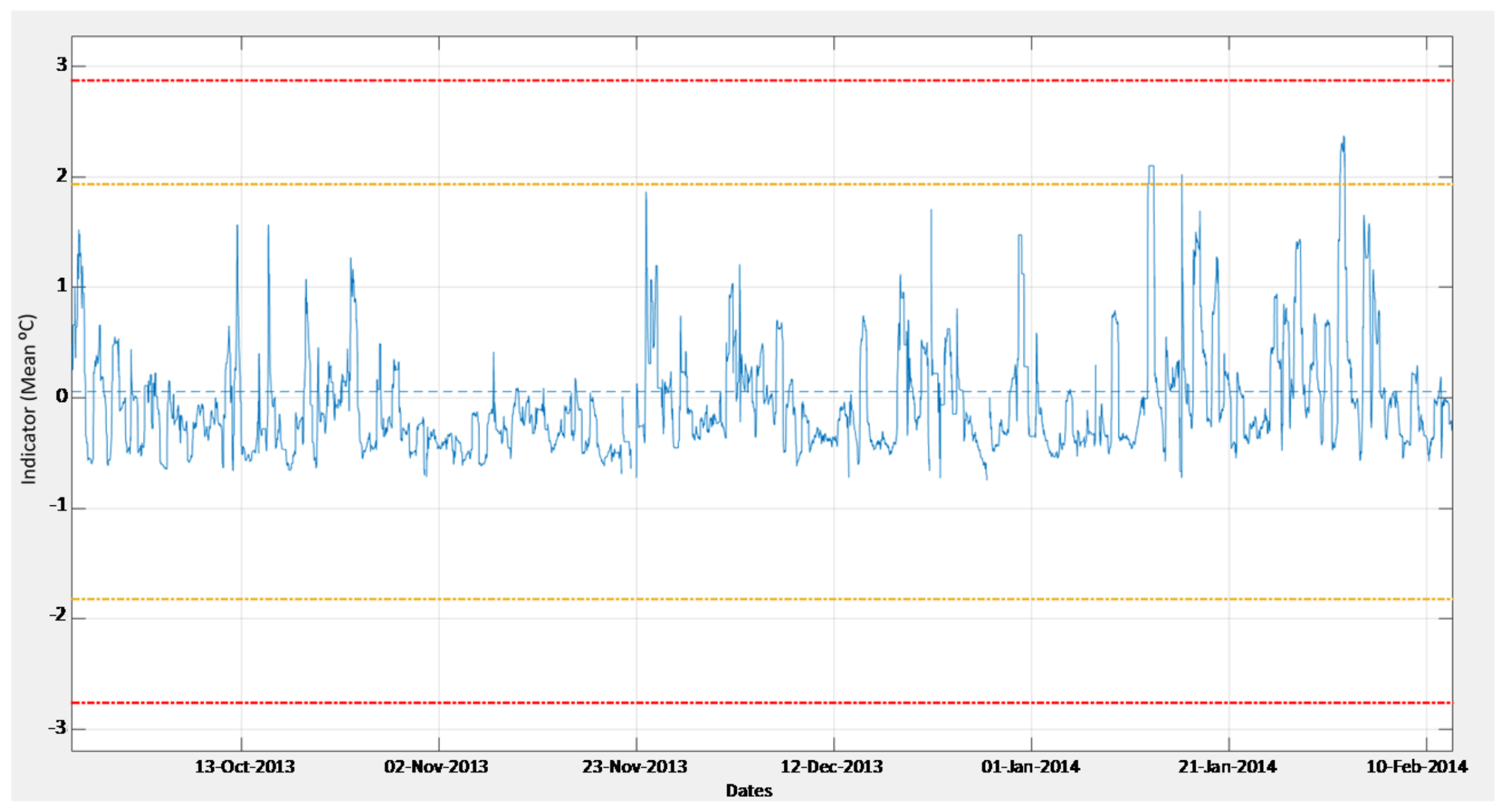Figure 13 shows that the mean value of the indicator (dotted blue line) stands at around zero, giving as a result a mean value similar to that obtained in calculation of the Generic Model of 0.12 °C (µ_Ind).

If no degradation occurs, the indicator may be expected to remain constant at this mean value. The standard deviation of the indicator (σ_Ind) has also been calculated and the levels of >2σ_Ind or <−2σ_Ind (Warning, in orange) and of >3σ_Ind or <−3σ_Ind (Emergency, in red) have been determined as the limits of normality. Thus, if the indicator exceeds these values at any point, a signal will be triggered indicating detection of possible malfunctioning.

Using the indicator values as a reference rather than the direct values of the remainders, removes the dependency on more precise models of behavior, since the reference changes. If the model were less well fitted, µ_Ind and σ_Ind would be different, making the deviation more problematic because it is the one actually used to determine the operating limits. Less precise models operate well in determining degradation, but would be more inclined to give false negatives. In order to resolve this conflict, more complex indicators will have to be developed that correct the deficiencies in the models. In real production situations, it is necessary to strike a compromise between model, indicator and false positives.

5. Case Study and Verification

For the case study, a critical failure (high impact or frequency of occurrence) was selected that was not detectable by the operation SCADA sufficiently in advance to be able to avoid it. The NDE bearing in a particular generator model triggered catastrophic failures that required the complete replacement of the generator, with the consequent loss of production. In such cases, production SCADAs do not detect malfunctions above alarm operating limits monitoring temperatures. With the methodology developed we have discovered that deviations of temperature outside the normality of the equipment can be detected several weeks in advance, without these having to surpass the temperature of normal operation of equipment (moment in which alarms are generated in the SCADA).

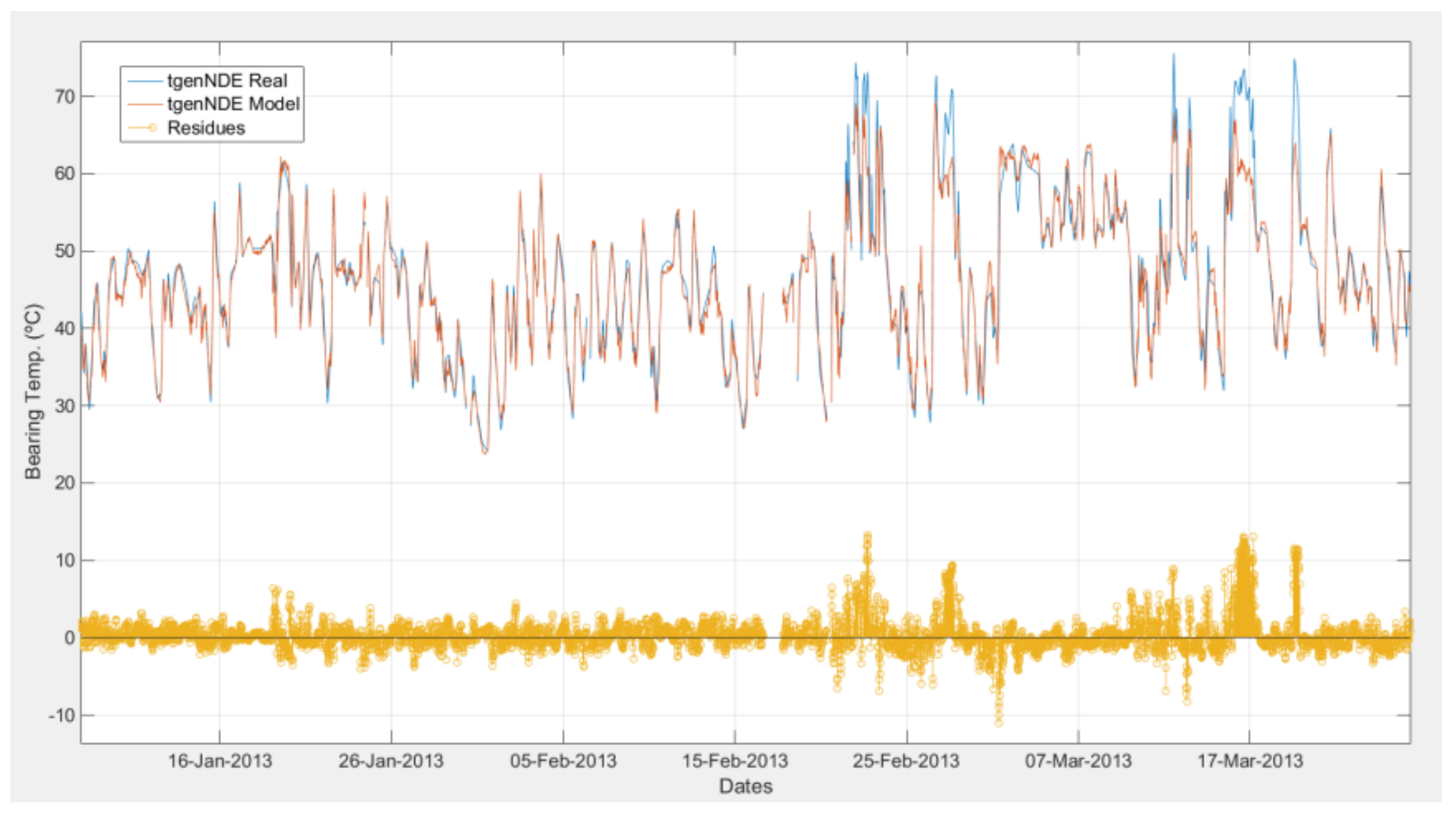
In a first approach to failure detection, before calculating the indicator, the NDE bearing temperature was plotted and compared to the expected temperature according to the Generic Model (Figure 14). It is observed that in the moments before the failure, the bearing presented extremely high temperature values in comparison with the value of the model, which generated higher residuals.

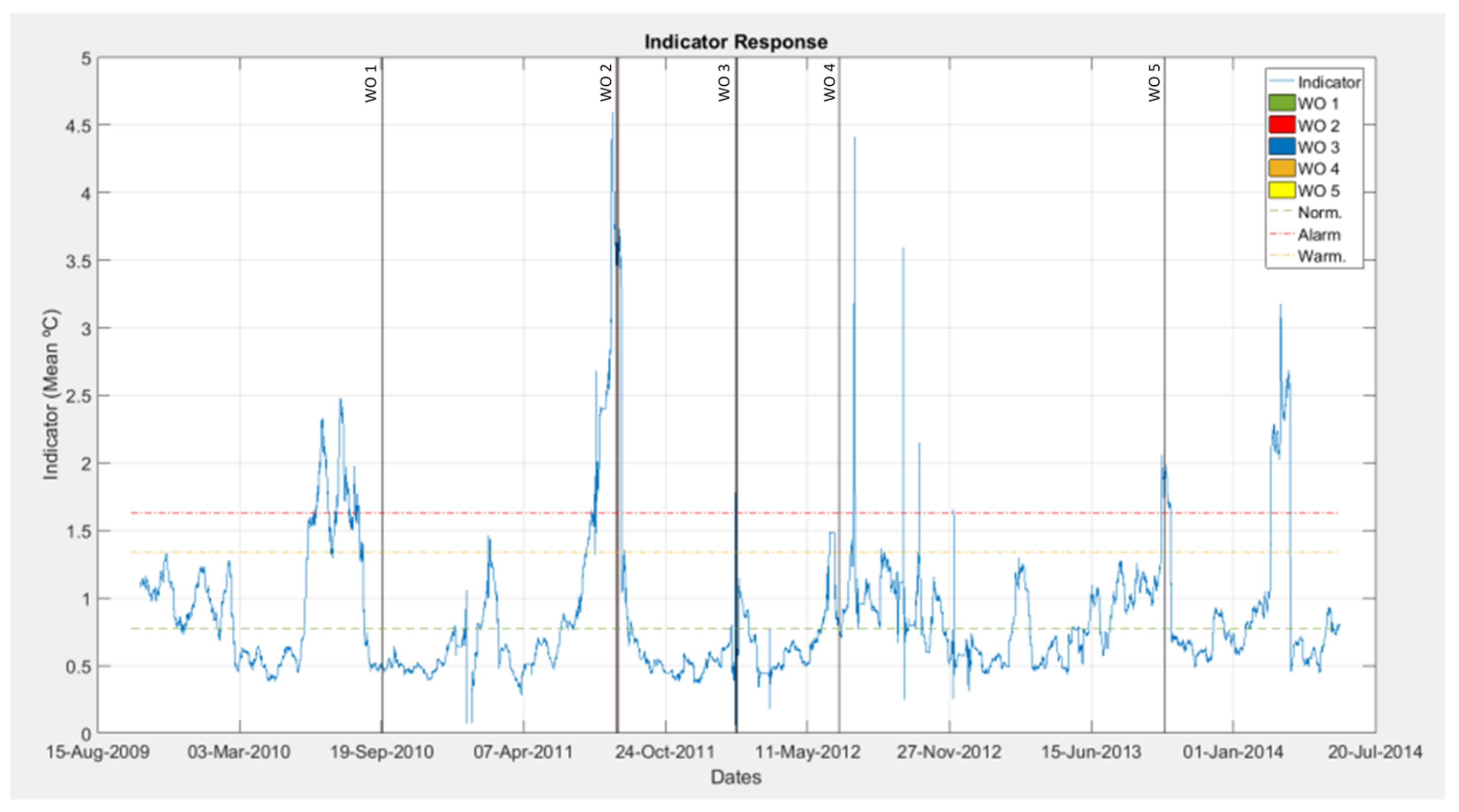
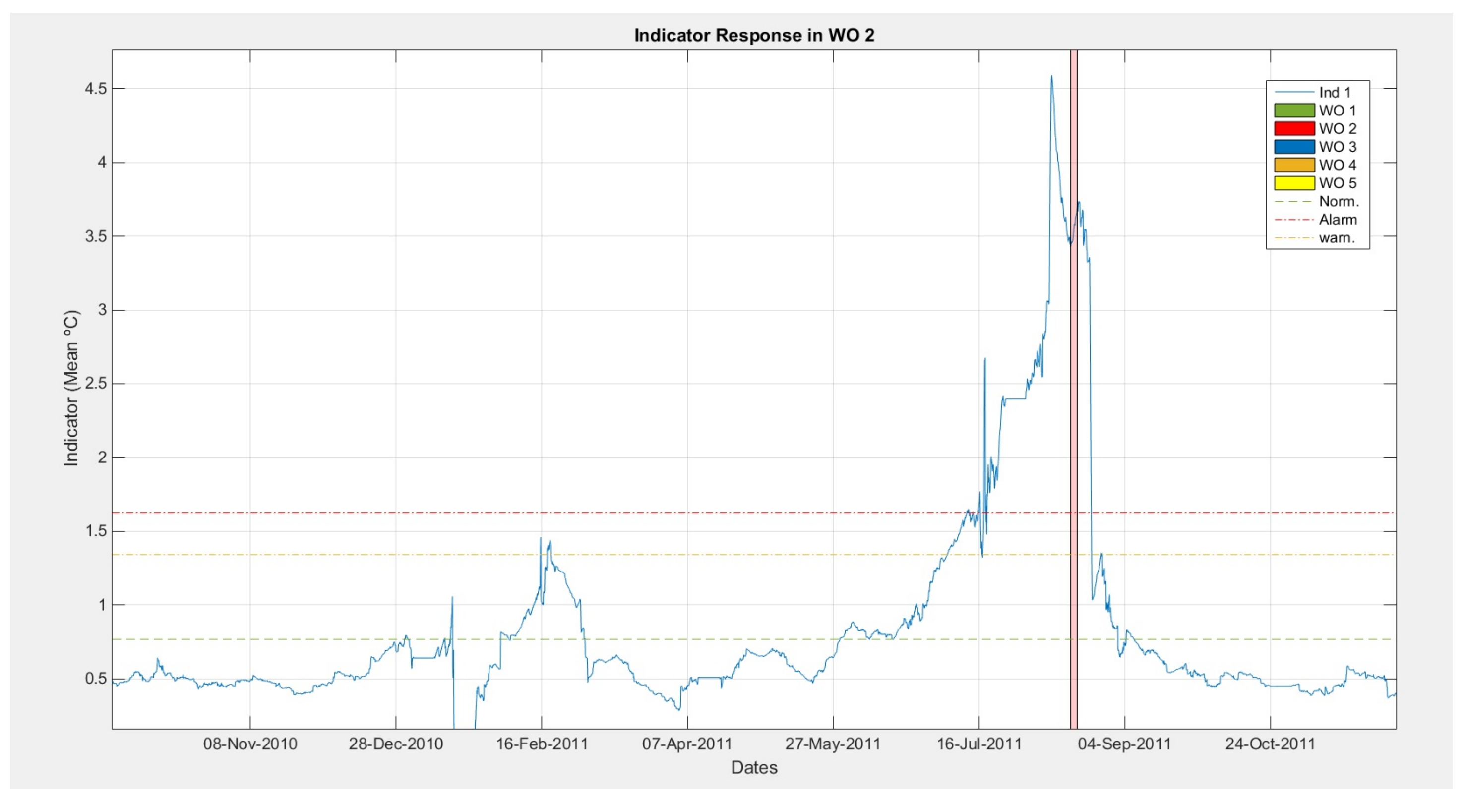
Finally, the indicator was calculated for the complete data log of the wind turbine for which the bearing had been replaced with WO 2. Figure 15 shows how the indicator reacts vigorously to other faults in the generator, which indicates that the use of a single indicator to determine a specific fault in a component could result in an error, i.e., malfunctioning in other components of the machine, as happens in WO 1 shown, which corresponds to the generator ventilators. It might be thought to be the bearing that has the fault, yet the increase in temperature here is not due to an intrinsic fault in the bearing, but to a fault in the unit’s cooling system. It is therefore necessary to develop a set of indicators for the different components and use them to train a system for diagnosing the origin of the fault. In other words, it is not only necessary to detect that something is malfunctioning in the generator, but also to be able to determine what is going wrong. Examining the reaction of the indicator before the bearing fault in Figure 16, there is a very vigorous reaction, exceeding the limits of normal operation of the indicator several weeks before, much more in advance than in [40].

Another important factor discovered, namely the recovery of the indicator’s state of normality. In other words, after repair, the indicator returns to normal values of around zero. This is very important since it demonstrates that the maintenance operation has been performed correctly and that the bearing (new in this case) once again shows normal behavior, even without having to retrain the model (the Generic Model continues to be used). The indicator calculated from the Generic Model has proved its validity for determining the degradation and detection of the malfunctioning of the unit, meeting the targets set, to the full satisfaction of the company for operating the unit.

6. Economic Results of Implementing the Model in Some Wind Farms Run by an Operating Firm

The models developed were validated by analyzing the results for somewhat over one year subsequent to implementation of the models. For a fleet of 14 wind turbines the mean annual breakage rate was one NDE bearing, with a mean duration of repair of 33 h stoppage and 41 h work attributed to the failure. In order to have a more representative ratio of the saving potential, a extrapolation of these figures was done to the total fleet of the operator, accounting with 739 wind turbines (with similar characteristics to the model analyzed), in this case mean annual breakages would come to 49 NDE bearings, requiring 1617 h of replacement work and a consequent 2009 h of labor. For all the fleet set, the mean output of all the farms is 2330 h equivalent at rated capacity per year, which translates into mean annual losses in power production of 860 MWh/year.

In economic terms, this signifies a total of €70.0 k/year, meaning that in the 20-year minimum lifespan of the wind turbines, the loss in these conditions would come to an estimated €1.40 m. Adding the cost of labor at an average of 41 h/year per repair, at €35/h, the cost is €1435 per repair, plus the cost of the materials involved, which comes to €5000 per repair, giving a total of €6435 per repair. Extrapolating again this to the other wind turbines, the total cost over the 20 years would come to €7.71 m for the 739 unit fleet. The savings would therefore be of between €1.4 m and €7.71 m, for that component and type of machine.

In the 18 months during which the methodology has been applied, and only for breakage of the NDE bearing, real replacement of these bearings has been halved, giving an effective estimated saving over 20 years of €4.55 m (

Table 4. Results of experience with the methodology and models developed for 20 years.

Cost Summary	14 Wind Turbines	739 Wind Turbines (Total Fleet)
Lost Energy	€28.4 k	€1.40 m
Spare parts and working hours	€128.7 k	€6.31 m
Total Costs without the methodology	€157.1 k	€7.71 m
Total Costs with the methodology	€64.35 k	€3.16 m
Total Estimated Saving	€92.75 k	€4.55 m

). No sensibility studies were developed, due to the fact that it would require the application of this methodology to a bigger fleet.

7. Conclusions

The main contributions of this paper can be summarized as follows:

(i)

The goodness of fit of different configurations of neural network and training algorithms were presented, in order to find a balance between resources in a productive environment, resulting Generic Models the most balanced solution. It was demonstrated that the TDNN are suitable for thermodynamic phenomena, although some other configurations improved the model results, the increase of resources do not make them desirable. It was also demonstrated the applicability of clustering techniques for the detection of aberrant data. Other issue that were determinant to dismiss the Specific Model, is the computational requirements to develop the methodology in a production environment with thousands of Specific Models. Moreover, Specific Models require continuous re-training after each replacement, Generic Models only need one training session when new models are included in the fleet. With all this, this methodology can be applied massively to any equipment from which operational data are available.

(ii)

Long term detection indicators were developed, offering excellent results for degrading symptoms detection and being able to detect failures within 2 month time in cases where the SCADAs are not able to detect anything. This is mainly thanks to the methodology developed to configure the indicator and its normal behavior bounds. These bounds are unique for each wind turbine.

(iii)

Finally, the ability of the state indicators to recover to values into the normal behavior bounds after correct reparations was made, what is really useful for evaluating the effectiveness of the maintenance task and even to estimate the moment when an event changed the behavior of the equipment.

In future woks this methodology could be extended to the rest of the components and/or signals of a wind turbine, starting with those critical components. More complex indicators associated with each failure mode, as well as on prognostic techniques could be implemented. Survival studies could associate a failure probability to the indicators. In addition, the combination with fuzzy logic to develop failure diagnosis systems, taking in consideration all the signals in the equipment would be desirable.