A New Scheme to Improve the Performance of Artificial Intelligence Techniques for Estimating Total Organic Carbon from Well Logs


1
State Key Laboratory of Coal Resources and Safe Mining, China University of Mining & Technology (Beijing), Beijing 100083, China
2
College of Geoscience and Surveying Engineering, China University of Mining & Technology (Beijing), Beijing 100083, China
*
Author to whom correspondence should be addressed.
Energies 2018, 11(4), 747; https://doi.org/10.3390/en11040747
Submission received: 12 January 2018
/
Revised: 9 March 2018
/
Accepted: 21 March 2018
/
Published: 26 March 2018
(This article belongs to the Special Issue Unconventional Natural Gas (UNG) Recoveries 2018)
Abstract
:Total organic carbon (TOC), a critical geochemical parameter of organic shale reservoirs, can be used to evaluate the hydrocarbon potential of source rocks. However, getting TOC through core analysis of geochemical experiments is costly and time-consuming. Therefore, in this paper, a TOC prediction model was built by combining the data from a case study in the Ordos Basin, China and core analysis with artificial intelligence techniques. In the study, the data of samples were optimized based on annealing algorithm (SA) and genetic algorithm (GA), named SAGA-FCM method. Then, back propagation algorithm (BPNN), least square support vector machine (LSSVM), and least square support vector machine based on particle swarm optimization algorithm (PSO-LSSVM) were built based on the data from optimization. The results show that the intelligence model constructed based on core samples data after optimization has much better performance in both training and validation accuracy than the model constructed based on original data. In addition, R2 and MRSE in PSO-LSSVM are 0.9451 and 1.1883, respectively, which proves that models established with optimal dataset of core samples have higher accuracy. This study shows that the quality of sample data affects the prediction of the intelligence model dramatically and the PSO-LSSVM model can present the relationship between well log data and TOC; thus, PSO-LSSVM is a powerful tool to estimate TOC.
1. Introduction
The correct evaluation of source rock plays an important role in oil and gas exploration and study, among which the evaluation of the abundance of the organic matter in the source rock is an essential part. The source rock evaluation involves many parameters that reflect the physical characteristics of the source rock, and the total organic carbon (TOC) content is identified as a basic and important index, which can represent the abundance of the organic matter [1,2,3]. Despite the most direct method of obtaining the TOC content, the laboratory core analysis is costly and time-consuming, by which limited TOC data can be obtained, and it is difficult to meet the current demands of source rock evaluations. With the rapid development of unconventional exploration of oil and gas, the continuous and accurate study on the TOC is very necessary. Well logging is characterized by high longitudinal resolution and the continuity of the data. Therefore, the TOC content predictions based on the logging parameters have been given priority by more and more researchers [4,5,6].
Many achievements have been made with the continuous improvements made by researchers in the predictions of the TOC data content [7,8,9]. The experiments and analyses, from which limited TOC data can be collected, are still necessary for the evaluation of the source rock [10,11]. Source rock is characterized by special logging response, and therefore organic matter has some specific geophysical logging responses. Moreover, there is a certain relationship between the TOC content and the logging parameters, such as the neutron, natural gamma, density, resistivity, and acoustic time difference. Beers et al. [12] and Schmoker J [13] calculated the TOC content by using the natural gamma well log, which was found to be suitable for calculating TOC from the source rock, which is rich in radioactive elements. Schmoker and Hester [14], Meyer and Nederl [15], and Decker et al. [16] calculated the TOC content using the density log curve, which could not predict the TOC content accurately, because there was no strong correlation between the density log curve and the TOC content. Autric and Dumesnil [17] calculated the TOC content using the acoustic time difference well log, which showed a better prediction when there was a strong correlation between the acoustic time difference and the TOC content. The establishment of TOC content prediction equations based on the single well log was greatly influenced by the physical differences in study areas, and it was found that the use of an empirical Equation is unfavorable to the correct prediction of the TOC content. Guo et al. [7], Hu et al. [5], Wang et al. [18], and Zhao et al. [19] calculated the TOC content by combining the resistivity with neutron porosity well logs, which was characterized by simplicity and convenience. However, the source rock maturity and the background value of the TOC content were different in different researcher areas and were found to leave a significant impact on the prediction.
Zhao et al. [20] and Kamali et al. [8] defined the clay content curve with the density and neutron porosity well logs, and then overlaid this curve with the natural gamma curve in order to calculate the TOC content. This method was found to be better than ΔlogR in the same study field. In order to improve the single well log’s prediction of the TOC content, Heidari et al. [4] selected multiple well logs to establish a multiple linear regression equation for the prediction of the TOC content. However, it was found that it was difficult to determine the related parameters due to the non-linear relationships among the well logs. There is a complicated non-linear function relationship between the logging information and the TOC content. Therefore, it is difficult to make simple linear regression be approximate to the real function relationship, and as a result, it is impossible to predict the TOC content accurately with the well log. In recent years, artificial intelligence has attracted researchers’ wide attention and has also been involved in many areas of research [21,22,23]. Actually speaking, the research showed that the artificial intelligence methods were quite close to nonlinear implicit functions. Otherwise, the existing research revealed that artificial intelligence methods were practical in terms of the prediction of TOC content based on well logs. The relational model between the logging parameters and TOC content has been established by using the neural network in order to predict the TOC content more accurately [6,8,9,24,25,26]. The involved algorithm and kernel function were closely related to the prediction accuracy. In fact, the prediction models of TOC content based on neural network method could not be established without real data. Due to the fact that the function relationship was established with real data, the prediction accuracy of the established models largely depended on the real data. In summary, no matter how perfect the artificial intelligence learning algorithm is, it could not be close to the function relationship between the real logging parameters and TOC content without the real data.
Considering the influence of the sample data on artificial intelligence modeling, it is necessary to process the sample data before modeling. It is required to delete the fuzzy or inauthentic data, and retain the sample data, which can accurately reflect the real function relationship and the modeling of the artificial neural network. Fuzzy c-means clustering (FCM) is a type of clustering algorithm, in which the grade of membership is employed to determine the degree that each data point belongs to a certain cluster [27,28]. In order to improve the classification accuracy of the fuzzy c-means clustering algorithm, it was proposed that the simulated annealing algorithm should be combined with the genetic algorithm to analyze the fuzzy c-means clustering, so as to classify sample data, and then to obtain the high-quality data. In the actual production, there are limited TOC content data from coring experiments. However, for the small sample data, in this study, the TOC content prediction model was established with a least square support vector machine (SVM) based on the sample data before and after the optimization. Then, in order to improve the prediction accuracy, a least square support vector machine model was established based on the particle swarm optimization (PSO-LSSVM) for the prediction of the TOC content. At the same time, a BP neural network model for the contrastive analysis was established, and a new method for the predictions of TOC content was proposed.
2. Theory and Methodology
2.1. Optimization of the Sample Data
2.1.1. Methodology of the Fuzzy c-Means Clustering Algorithm (FCM)
In this study, the was assumed to be data samples, c () was the number of types of data samples; were the types; U was its similar classification matrix; were the cluster center of each type; and was the degree of membership of to , abbreviated as . Then, the expression of the objective function was as follows:
In Equation , represents the Euclidean distance, which is used to measure the distance between in the ith sample and central point of the kth, indicates the number of the sample’s characteristics, is the weighted parameter, and its value range is . A fuzzy c-means clustering method was used to find a new optimal type of classification; it made this classification get the minimum function value . It required that the sum of the membership values of one sample to each cluster be 1, which confirmed the following equations:
Equations (3) and (4) were used to calculate the grade of membership to the and the cluster centers of c, respectively, which was as follows:
If it was assumed that ; then, for all “i”s, , :
The cluster center and grade of membership of the data were repeatedly adjusted with Equations (3) and (4), and then were classified. In the case of algorithm convergences, the theoretical value of the grade of membership between each cluster center and sample to each model was obtained, and the division of the fuzzy clusters was completed. Although the FCM is identified as high-speed searching, it was limited to searching something locally, and it was also found to be particularly sensitive to the initial value of the cluster center [29]. Therefore, if the initial value could not be properly selected, then it fell into the local minimum.
2.1.2. Methodology of the Simulated Annealing Algorithm (SA)
A simulated annealing algorithm was successfully applied to combining optimization, based on the fact that the global optimal solution, or nearly global optimum, can be searched by simulating the annealing process of the high-temperature objects [30]. The process of the simulated annealing algorithm was as follows:
(1) was chosen as the initial state, and was set; it was assumed that the initial temperature was , and was set;
(2) was set; and referred to the Metropolis sampling algorithm; the state was returned as the current solution of this algorithm, and ;
(3) The temperature was lowered with a certain method, for example: , where , ;
(4) The termination conditions were checked, and if they were suitable, then came to step (5); or came back to step (2);
(5) If the current solution was the optimum solution, the result was gained as output, and the process was terminated.
2.1.3. Methodology of the Genetic Algorithm (GA)
(1) Encoded mode: In the genetic clustering algorithm, the parameters to be optimized were c initial cluster centers with binary coding. Each chromosome consisted of c cluster centers. For the m–dimensional sample vector, the number of variables to be optimized was . Assuming that each variable used the k-bit binary coding, and the length of chromosome was the binary code string of ;
(2) Fitness function: This was the scale that was used to weigh the pros and cons of the individuals. Its function was like weighing the organism adaptation to environment. Each individual regarded the as the objective function from Equation (1), and the smaller the was, the larger the adaptation value of the individuals was. Therefore, in the fitness function, the distribution function of fitness values: was employed;
(3) Selection of the operator: The stochastic universal sampling was used;
(4) Crossover operator: The single-point crossover operator was used;
(5) Mutation operator: The number of variant genes will appear with a certain probability, and the variant genes will be selected out using a stochastic method. If the selected gene is encoded as 1, it will be 0, or it will be 1.
2.1.4. Flowchart of the SAGA-FCM Algorithm
This flow of fuzzy c-means clustering algorithm based on a simulated annealing genetic algorithm is shown in Figure 1. Logging parameters were used as the characteristic index of sample data in order to classify the pros and cons of the sample data. The procedures were as follows:
(1) The various control parameters were initialized, including the weighted index b in the fuzzy c-means clustering algorithm, maximum iterations N, termination tolerance D of the objective function, size of population individual , maximum of evolutional generation , crossing probability , variation probability , initial temperature of annealing , cooling efficient of temperature, and terminal temperature ;
(2) The clustering centers were randomly initialized, and the initial population Chrom was generated; for each clustering center, Equation (3) was used to calculate the grade of membership of each sample and the adaptation value of each individual, here ;
(3) The loop count variable was set as ;
(4) The abnormal operations were implemented in the sample Chrom, such as the selections, crossovers, variations, etc., and Equations (3) and (4) were used to calculate the c clustering centers and grade of membership of each sample for the newly generated individuals, as well as the adaptation value of each individual. If , then the old individuals were replaced by new individuals; or, the new individuals were accepted with a probability of , and the old individuals were abandoned;
(5) If gen < MAXGEN, and gen = gen + 1, then come to Step (4); or come to Step (6);
(6) If , the algorithm would be successfully completed, and the global optimal solution would be gotten; or, the cooling operation would be implemented, leading to Step (3).
2.2. Methodology of the Least Square Support Vector Machine
A SVM (support vector machine) is a type of new machine learning method proposed by Vapnik [31]. For SVM, based on the statistical learning theory, the minimization principle of structural risk was adopted to improve the generalization ability of small sample data, and defects such as the long training time of the neural network, randomness of the training results, over-learning, etc., were gotten rid of. Therefore, SVMs can be widely used to build complicated non-linear models.
LSSVM is a derivative method of SVM, which was proposed by Suykens [32] and successfully introduced the least square estimation into the SVMs. Compared with the inequality constraints and quadratic programming of the standard SVMs, it solves the linear equation problem, simplifies the operation process, and improves the calculation of speed and accuracy. In the LSSVM, the square-error item is regarded as the optimization target, and the equality constraint is regarded as the constraint condition. This study utilized the regression form of LSSVM, and its main principles are as follows:
For the training sample (with size N), in which was regarded as the input and the output is , its linear regression function in the low-dimensional space was as follows:
in which is the weight vector and is the offset. The regression function of this sample in the high-dimensional feature space was as follows:
in which the nonlinear transformation is the mapping from the low-dimensional space to the high-dimensional space. For LSSVM, in accordance with the structural risk minimization principle, the square-error loss function was selected from the optimization targets; the regression problem changed into a quadratic optimization problem as follows:
in which is the slack variable and is the regularization parameter. Its constraint condition was as follows:
In order to solve the problem about optimization, a Lagrange function was introduced:
in which represents the Lagrange multiplier. The following Equation could be obtained according to the KKT (Karush-Kuhn-Tucker) optimization conditions:
The definition kernel is as follows:
By eliminating the and in Equation (10), the quadratic optimization problem could be transformed into solving the linear Equation (12) as follows:
The above and in linear equations could be solved with a least square; then, the regression function of LSSVM could be obtained as follows:
2.3. Methodology Parameter Optimization of the LSSVM
Particle swarm optimization (PSO) is a global optimization algorithm [33]. The optimal solution is gotten by using the indirect communication among individuals with this method based on the simulation of the foraging process of bird flocks.
In the D-dimensional solution space, the possible solution of each optimization is regarded as one “particle” in the space, and m particles compose a community. Also, is defined as the current location of the particle i; is the current flying speed of the particle i; are the optimal positions up to current iteration. is the optimal position searched by the entire particle swarm up to current iteration. Each particle follows the optimal position to search in the solution space. The renewal equation for the speed and position of the particle i is as follows:
in which and are the speed and position of the particle i in the kth iteration of the d-dimension, respectively; and are the positive acceleration coefficients (or learning factors); and are two random numbers in [0, 1]; and and are the optimal position of the individuals, and the global optimal position of the entire community of the particle i in the D-dimension, respectively.
In order to improve the learning ability and generalization ability of LSSVM, this study used a PSO algorithm to realize the global optimization of the LSSVM parameters, and the optimization process is shown in Figure 2.
2.4. Methodology of the Back-Propagation Neural Network
The artificial neural network is made up of artificial neurons connecting with each other. The network essentially realizes a mapping function from input to output. Also, mathematical theory has proven that the artificial neural network has the ability to realize any complicated non-linear mapping [34,35,36,37,38,39]. A BP neural network is essentially an error back-propagation BP learning algorithm. It has the ability to correct the error of connection weights and thresholds in various layers of the network from back to front according to the differences between the actual output and expected output and then from front to back. Repeating this process can minimize the errors to end [34,37,38]. For this method, the unknown system is regarded as a black box, in which the input and output data of a system sample are used to train the BP neural network to express the unknown function. The essence of defining this unknown function is to solve the minimum value of the error function. Training was based on applying core samples data repeatedly until the minimum of the error was obtained. At this time, the connection weights of the various layers and the threshold of nerve cells in each layer, along with other information obtained through the training were saved as knowledge, and then the training ended. Then, output of the system was predicted with the trained BP neural network.
3. Data Analysis and Optimization
3.1. Study Area
In recent years, PetroChina, Sinopec, and Shell, among others, have conducted many studies and production processes in the Ordos Basin. Some studies have shown that the organic matter in most areas of the basin is at the mature stage [40,41,42,43,44]. The Ro (vitrinite reflectance) value ranges from 0.85% to 1.20%; Types I and II of kerogen are the main types in this study area, and the TOC content of the organic-rich shale ranges from 0.23% to 32.86%. The position of the Ordos Basin in China is marked with a red rectangle in Figure 3a, and Well E1 is located in the north-central part of the Ordos Basin as is shown in Figure 3b.
In this study, TOC was measured with a LECO CS-400 carbon sulfur analyzer (LECO CS-400, LECO Corp., Saint Joseph, MO, USA) (combustion at temperatures over 800 °C). A total number of 70 TOC data points were obtained from laboratory tests. On September 14, 2015, mud drilling technology was used for the drilling of Well E1 in Tabudai Village of Wulan County, which is a suburb of Wushenqi City. The drilling was completed on 27 October 2015, with a drilling depth of 2284 m. On October 28, the logging operations were carried out. The location of the drilling in the study area is shown in Figure 3b. Logging equipment is from the logging system of COSL (China Oilfeld Services Limited, Beijing, China); logging method is from Well E1 and includes the caliper logging, spontaneous potential, natural gamma-ray spectroscopy, array acoustic, dual lateral resistivity, lithology density, and neutron porosity logs, of which all the logging curves displayed excellent qualities. Table 1 shows the logging parameter data of Well E1, along with the TOC content data that were analyzed in the core experiment.
3.2. Data Analysis
The relationship between the logging parameters and the TOC content differs dramatically in different areas. Also, it cannot be guaranteed that the empirical Equation established in previous studies to calculate TOC content can get the same prediction effects [12,17]. In different study areas, the function relationship between the logging parameters and TOC content was also found to be different [5,7].
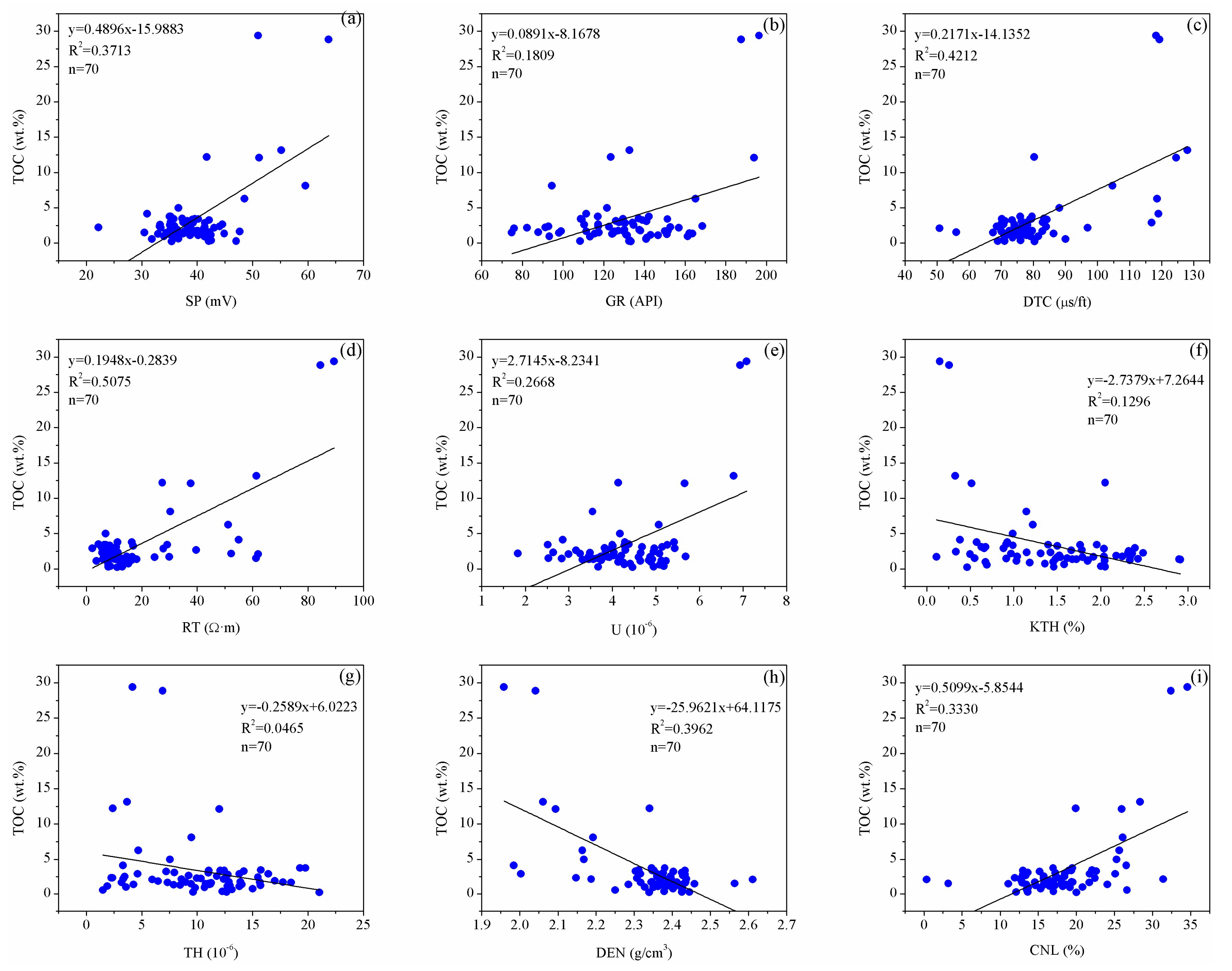
Therefore, in order to define the relationship between the well log and TOC content, this study obtained a simple linear regression relationship between the well log and TOC content through a cross-plot analysis for the TOC content of the samples and well log. The coefficient (R2) was regarded as the index to judge whether the correlation between each well log and TOC content was strong or not. Figure 4 shows the cross plots between the logging parameter and TOC content of Well E1. It can be seen that there is a positive correlation among the well logs of the spontaneous potential, gamma ray, acoustic time difference, resistivity, uranium and neutron porosity, and TOC content, and their coefficients of determination are 0.3713, 0.1809, 0.4212, 0.5075, 0.2668, and 0.3330, respectively. However, there was a negative correlation among the well logs of the potassium, thorium, and neutron porosity and the TOC content, and their coefficients of determination are 0.1296, 0.0465, and 0.3962, respectively. After comparison, when the simple linear regression of the well log and TOC content is made, the resistivity curve has the largest coefficient of determination, while the thorium curve has the smallest coefficient of determination.
In addition, this study conducted a correlation analysis for the well log and TOC content, to calculate the correlation between each well log and the TOC content. The calculation Equation is as follows:
in which r is the correlation coefficient; and are the average value of logging parameters, respectively; xi and yi are the corresponding logging observation values of the ith coring sample point, respectively.
Table 2 shows the correlation coefficient matrix obtained by calculation. It can be seen that the correlation coefficient between the resistivity curve and the TOC content was high (0.7124). Otherwise, there is a high coefficient of correlation among the spontaneous potential, acoustic time difference, density, neutron porosity, uranium curve, and gamma ray curve, and the TOC content.
In summary, it was found from the analysis for the cross-plot and coefficient of correlation between the well log and TOC content that there was no one-to-one correspondence function relationship between any aforementioned well logs and the TOC content. However, the sensibility of different well logs to the TOC content was significantly different. This study analyzed the log response characteristics of the TOC content, as is shown in Table 3.
3.3. Data Optimization
The 70 sample data of the wells were divided into two types according to the fuzzy c-means clustering analysis. One type was the data that best reflected the function relationship between the TOC content and the log curve, which was called the high-quality sample point. The other type was the data that were named the low-quality sample point, because they could not reflect the function relationship between the TOC content and log curve. The aforementioned nine types of log curves were regarded as the sample classification index. Since the log data had different dimensions and orders of magnitude, it was necessary to preprocess through normalization to guarantee the classification effect. The normalization processing Equation was as follows:
in which is the index value after normalization; is the lth index of the nth sample; and and represent the maximum and minimum value of the sample of the lth index, respectively.
Following the normalization, the sample data were classified using a fuzzy c-means clustering method based on a genetic simulated annealing algorithm. The algorithm in this study involved the control parameters that are shown in Table 4.
In Table 4, b is the weighted index and controls the distribution of the grade of membership and the fuzzy degree of clusters; N represents the maximum number iterations; D represents the termination tolerance of the objective function; sizepop indicates the population size; MAXGEN represents the maximum number of evolution; Pc is the crossover probability; Pm represents the mutation probability; T0 is the initial annealing temperature; k represents the cooling coefficient; and Tend represents the end temperature.
The samples were classified into high and low-quality samples. Also, the grade of membership of each sample to these two classes was obtained through calculation. Comparing the grades of membership of these two classes, the class with a larger grade of membership was the grade of the sample. Table 5 shows the matrix of the grade of membership for the samples. The values of HQ and PQ for each sample point were calculated by SAGA-FCM method as list in Table 5. If the HQ value less than the PQ value, the data is classified as low-quality data. As can be seen from Table 5, there were 61 high-quality sample points in total, while the remaining nine sample points were low-quality sample points.
A cross-plot and a coefficient of correlation analysis were constructed for the 61 high-quality sample data. As is shown in Table 6, comparing the analysis results of the sample data before optimization (Figure 4 and Table 2), it was found that the coefficient of determination and that of correlation were both greatly improved. This study analyzed the coefficient of determination before and after the optimization of the sample data. The change rate of R2 were calculated by the following equation:
in which is the R2 of optimization samples, is the R2 of original samples, and G is the change rate of R2 before and after the optimization of the sample data.
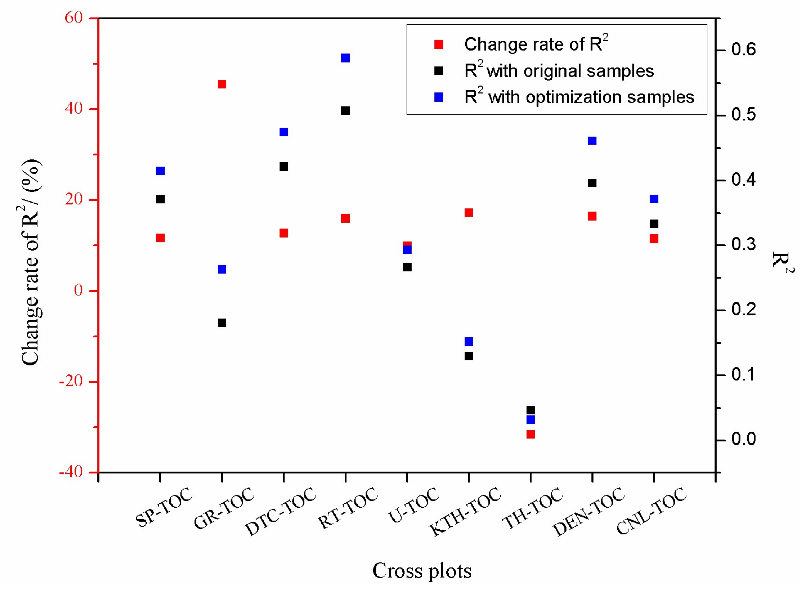
When the G > 0, it means that the optimization is effective. While the G < 0, it means that the optimization is invalid. As shown in Figure 5, it was obvious that the coefficient of determination (R2) for the well log and the simple linear regression of the TOC content after optimization of sample data were greatly improved. For example, the natural gamma ray curve had the largest change in coefficient of determination (the change rate of R2 for GR-TOC is 45.4395%). Since there was almost no correlation between the thorium curve and the TOC content, the coefficient of determination showed a negative change (the change rate of R2 for TH-TOC is −31.6129%). The coefficient of determination (R2) for the spontaneous potential, acoustic time difference, resistivity, uranium curve, potassium curve, density curve, and compensate neutron curve all showed positive change. From Figure 5, taking SP-TOC for example, the R2 of SP-TOC with original samples data is 0.3713, and the R2 of SP-TOC with optimization samples data is 0.4146. Then, the change rate of R2 for SP-TOC is calculated by Equation (18), which is 11.6617%. Finally, the change rates of R2 for DTC-TOC, RT-TOC, U-TOC, KTH-TOC, DEN-TOC, and CNL-TOC were calculated, respectively, and they were 12.7018%, 15.9803%, 9.8951%, 17.2068%, 16.4311%, and 11.5315%, respectively. The results illustrate that the sample data optimization is effective generally.
4. Results
4.1. Model Establishment
After the analysis on the correlation between the TOC content and the log curve, as well as the optimization of sample data, for comparison, this study established three types of TOC content prediction models based on the sample data. These three models were the least square support vector machine (LSSVM) model, the least square support vector machine model based on the particle swarm optimization (PSO-LSSVM), and the back propagation neural network (BPNN) model, respectively.
4.1.1. LSSVM and PSO-LSSVM Models
The nine types of log curves were regarded as the related logging characteristic parameters of the TOC content, and then the LSSVM method was used to establish the non-linear model between the logging parameters and the TOC content. Meanwhile, the input data and output data of the model were the logging parameters and TOC content, respectively. Finally, this non-linear model was used to predict the TOC content.
The non-linear model structure was established between the logging parameters and TOC content with the LSSVM method as follows:
The Gaussian radial basis function (RBF) was chosen to be the kernel function of the model, and its expression Equation was as follows:
in which is the center of the kernel function and is the shape parameter of the kernel function.
Then, if the regularization parameter in the structural risk calculation expression in Equation (7), and the width parameter of the kernel function in Equation (20) is calculated with the PSO algorithm; this will become the PSO-LSSVM model.
4.1.2. Back-Propagation Neural Network Model
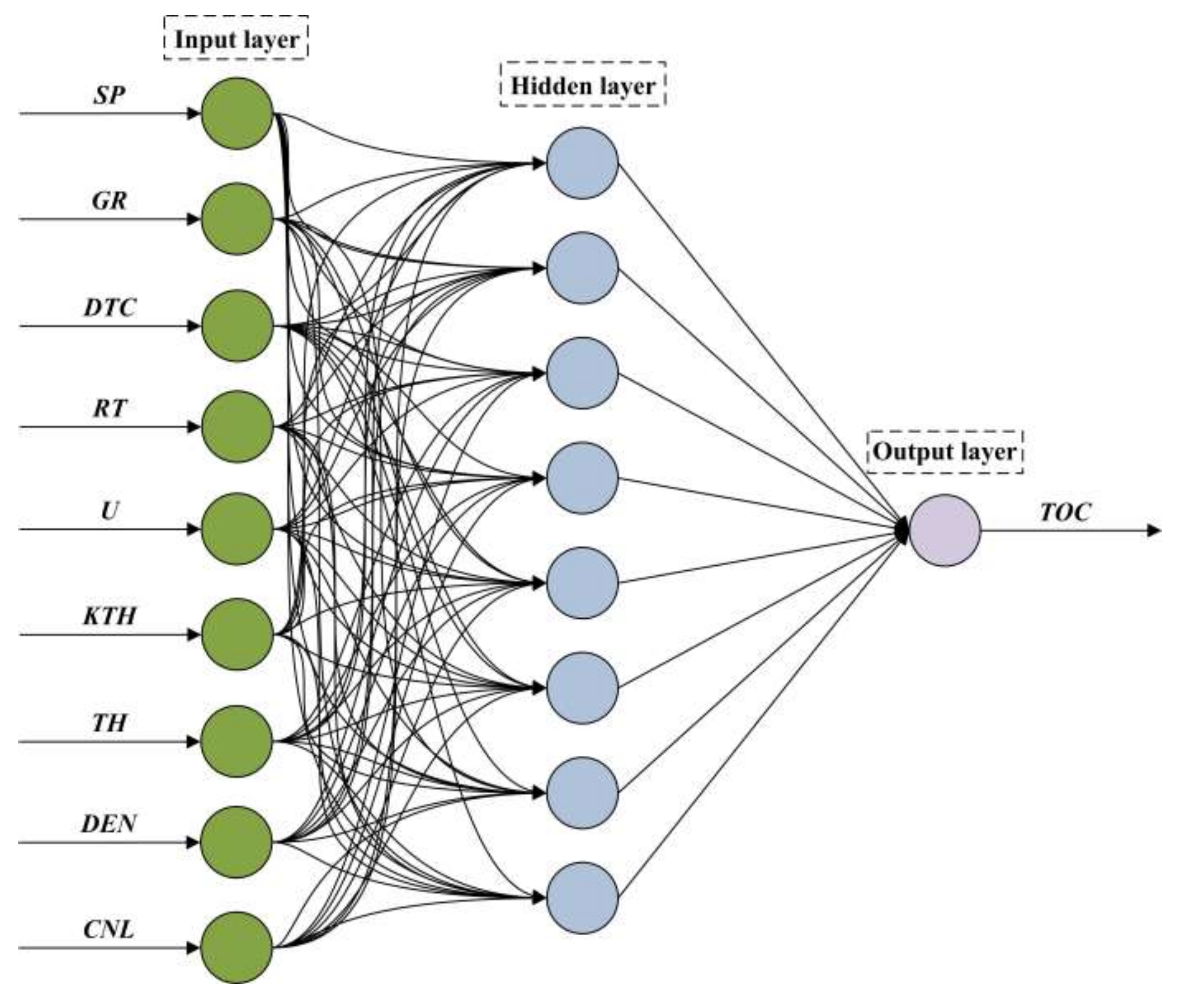
The Kolmogorov theorem stated that one three-layer neutral network can approximate a continuous function at an arbitrary precision. Therefore, this study established a three-layer BP neutral network containing only one hidden layer. This network consisted of an input layer, hidden layer, and output layer. The input-dependent variable was the nine types of well logs, and therefore the number of nerve cells at the input layer was nine. The input-dependent variable was the TOC content, and therefore the number of nerve cells at the output layer was one. The optimum value range [3,13] of the number of nerve cells in the hidden layer can be determined by the empirical Equation (Equation (21)). Then, it was determined through the traversal method that the number of the hidden neurons was 8. As shown in Figure 6, this study established the BP neutral network model of the 9-8-1 structure as follows:
in which H is the number of nerve cells in the hidden layer, I is the number of nerve cells in the input layer, O is the number of nerve cells in the output layer, and is the constant.
A hyperbolic tangent function was selected as the excitation function, and a learning method with a dynamic learning rate was used. The training error converged quickly after the iteration. The established BP neutral network prediction model for calculating the TOC content was as follows:
in which xi represents the nine well logs in the network input layer; wij and a are the weight coefficient and threshold from the network input layer to the hidden layer, respectively; vjk and bk are the weight coefficient and threshold from the hidden layer to the output layer, respectively; tanh is the hyperbolic tangent function, which is the excitation function of the hidden layer in the network, and its domain of definition and value range are (−∞, +∞) and (−1, +1), respectively; n = 9 is the number of feature vectors in the input layer; m = 8 is the number of nodes in the hidden layer; and k = 1 is the number of nodes in the output layer.
4.2. Model Performance
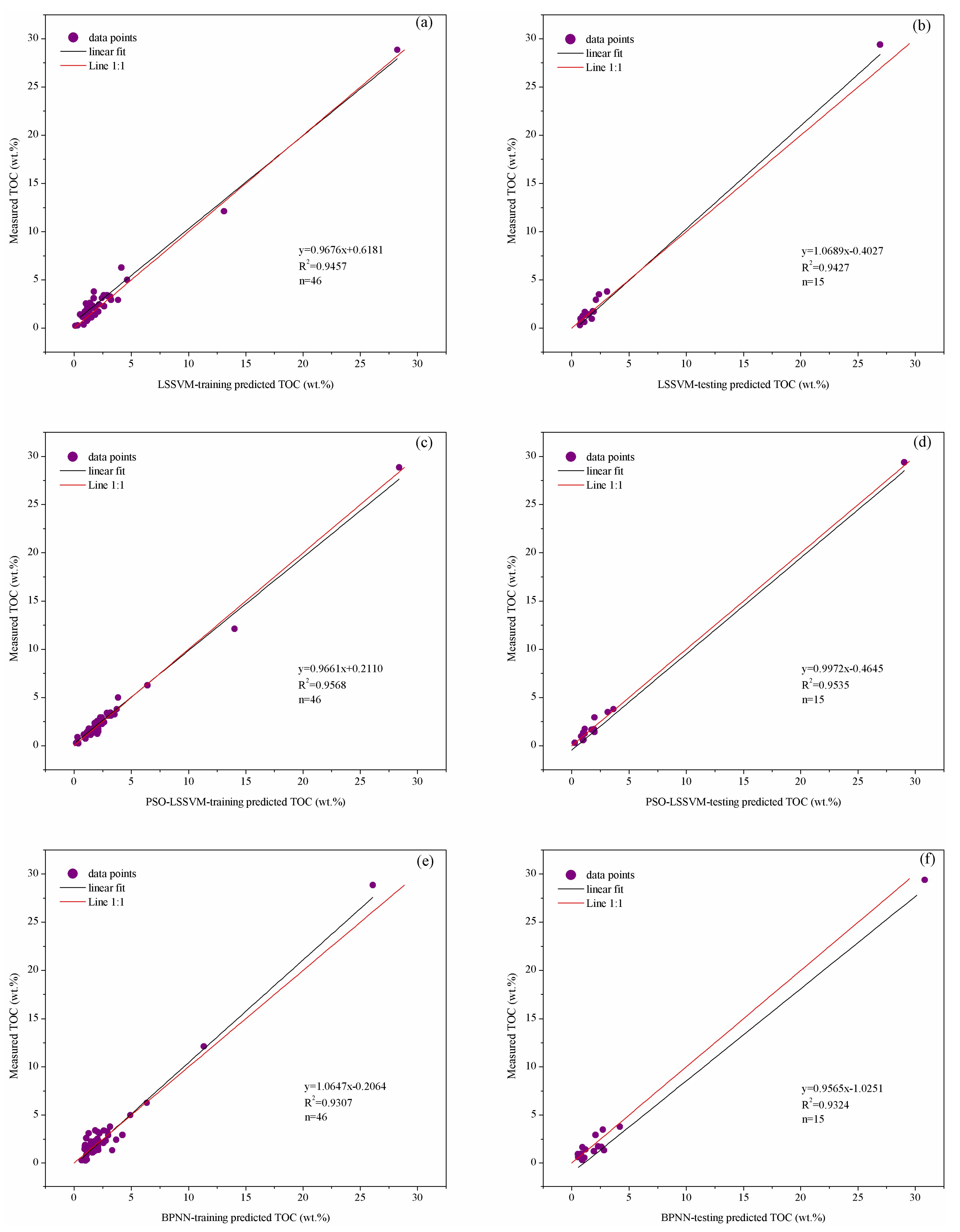
This study implemented the training and trial analysis for the aforementioned three types of TOC content prediction models on the basis of the original sample data and the optimized sample data, respectively. Also, this study randomly divided the data set into the training subset and testing subset, where the training subset accounted for three quarters, while the testing subset took up one quarter of the total. The cross-plots were made about the actually measured TOC content and the predicted TOC content to analyze the model’s prediction effect. The coefficient of determination was used as the evaluation index. Figure 7 shows the model prediction effect based on the original sample data, while Figure 8 shows the model prediction effect based on the optimized sample data. Comparing the prediction effects of models in Figure 7 and Figure 8, it was noticed that the effects of TOC prediction with the optimized sample data had improved dramatically. The determined coefficients of training part and test part in the model of LSSVM increased from 0.8706 and 0.8715 to 0.9457 and 0.9427, while those in BPNN increased from 0.8464 and 0.8857 to 0.9307 and 0.9324. The comparison proved the importance of favourable data set to artificial intelligence learning machine. Otherwise, in general, for the determined coefficients of the three types of TOC content prediction models in the study, the optimized model based on PSO-LSSVM had the largest coefficient and followed by the model that is based on LSSVM, while the BPNN had the smallest coefficient.
In addition to the coefficient of determination, the root-mean-square error (RMSE) and the variance accounted for (VAF) were used as indexes to compare the model’s prediction effects. These indexes could be used to measure the degree of closeness between the model’s prediction result and the actual value. The root-mean-square error (RMSE) was used to weigh the deviation between the model prediction value and the actual value. The more favourable the model prediction effect was, the smaller the root-mean-square error (RMSE) was, and its calculation Equation was Equation (23). The VAF was usually used to evaluate the accuracy of models by comparing the model prediction value and the actual value. Its calculation Equation is Equation (24), as follows:
In Equations (23) and (24), represents the model prediction data, represents the actually measured data, and n indicates the number of samples that were used for the network training or testing.
Table 7 showed the results of the RMSE and VAF through calculations. Based on the optimized sample data training, RMSE became smaller, while VAF became larger, which indicated that the prediction effect was better. In addition, RMSE in the PSO-LSSVM model was the smallest regardless of the basis of the original sample data or optimized sample data, which indicated that this model had a better prediction effect compared with LSSVM and BPNN models.
4.3. Model Validation
It was found from the aforementioned analysis that the prediction effect of the intelligent model was greatly influenced by the quality of the trained data set. This study used the optimized sample data set to train the LSSVM, PSO-LSSVM, and BPNN models and then used each model to predict the TOC of Well E1.
In addition, in order to make a visual comparison of the pre-quality, Figure 9 details the comparison between the TOC prediction value and the actually measured TOC value of the different models. The left three curves in Figure 9 are the well logs, while the right three curves are the corresponding model prediction the TOC curves. The purple dash represents the TOC prediction result of the LSSVM model, the green dash represents the TOC prediction result of the PSO-LSSVM model, and the blue dash represents the TOC prediction result of the BPNN model. Then, comparing the right three curves in Figure 9, it could be concluded that the prediction result of the PSO-LSSVM model was more consistent with the actual measured TOC result of the core samples.
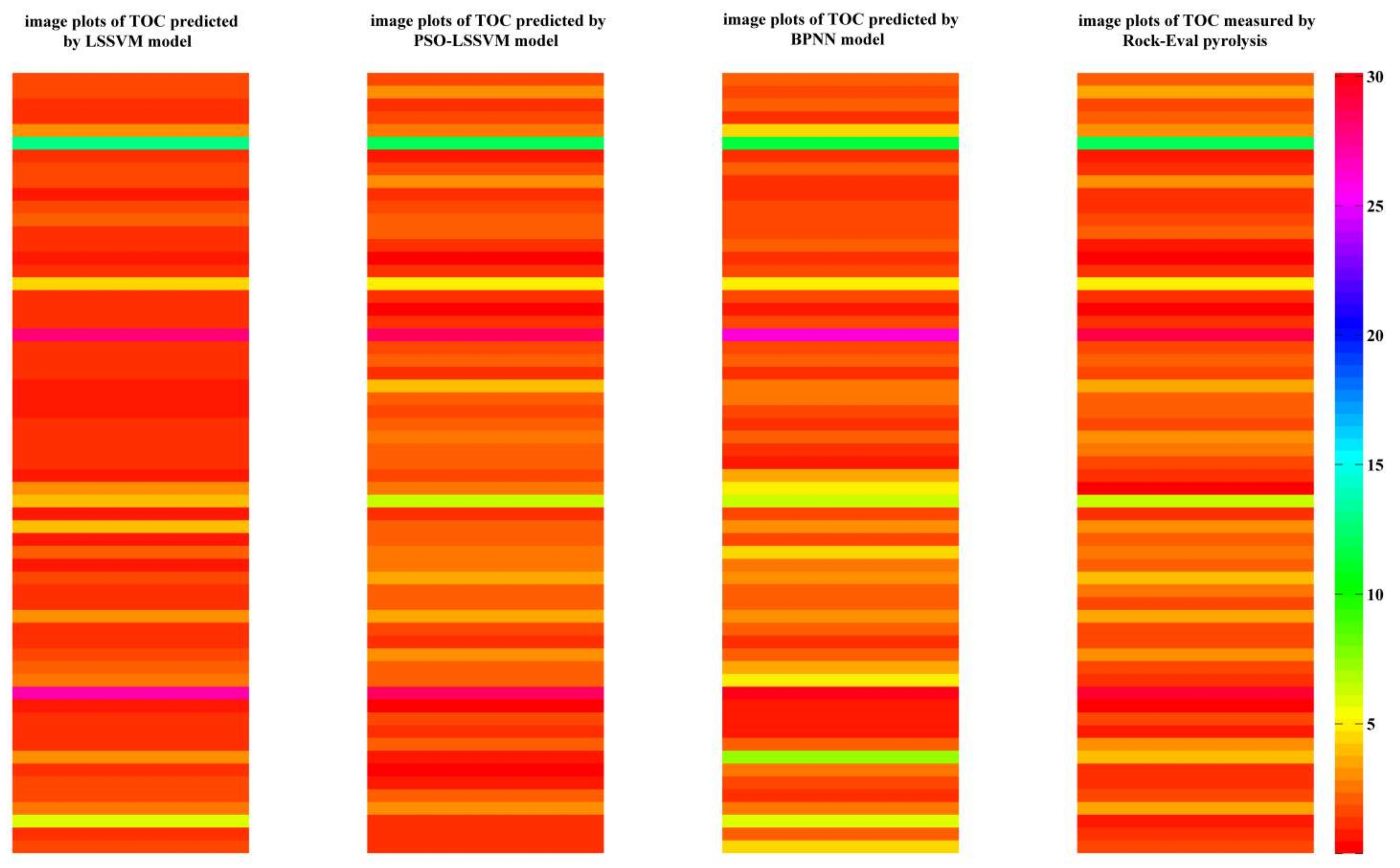
Figure 10 shows the comparison between the actual measured TOC and the model predicted TOC. It can be clearly noticed that the PSO-LSSVM model in this study had a better prediction effect. In addition, according to the R2, RMSE, and VAF results calculated in the Table 8, it was proven that the prediction result of the PSO-LSSVM model was more consistent with the actual measured TOC (R2 = 0.9451, RMSE = 0.3383). Also, the PSO-LSSVM model was more suitable for the TOC prediction when compared with the other methods.
5. Conclusions
In recent years, artificial intelligence technique has become an effective tool in oil and gas exploration, which makes up the defects of the traditional methods of evaluating TOC. In the study, at first, the high-quality samples data were distinguished from the samples data set from Ordos Basin, China by using the fuzzy c-means clustering algorithm (FCM) in combination with the simulated annealing algorithm (SA) and the genetic algorithm (GA), named the SAGA-FCM method. Then, original samples data and optimization samples data (high quality data) were analyzed by using correlation analysis and the linear regression method, in which R2 was regarded as the index of evaluation. The results showed that the relativity between well logging parameters of optimization samples data and TOC was better. Next, TOC prediction models, which were based on original samples data and optimization samples data, respectively, included the LSSVM, PSO-LSSVM, and BPNN models. According to error analysis using R2, RMSE, and VAF criteria, the obtained results showed that the intelligence model based on optimization samples data had much better performance in both training and validation accuracy, because it could reflect the functional relationship between the well logging parameters and TOC genuinely. Finally, the models established in this study were comparable. It can be seen that TOC could be predicted more accurately with PSO-LSSVM model than with LSSVM and BPNN models, and it had a more favorable effect from visual comparison between the prediction results and the data of measured TOC, as well as error analysis (R2, RMSE, and VAF).
Acknowledgments
This research is financially supported by the National Science and Technology Supporting Program (2012BAB13B01), National Key Scientific Instrument and Equipment Development Program (2012YQ030126), Coal United Project of National Natural Science Foundation (U1261203), China Geological Survey Project (1212011220798), National Science and Technology Major Project (2011ZX05035-004-001HZ), National Natural Science Foundation of China (41504041), and China National Key Research and Development Program (2016YFC0501102).
Author Contributions
Pan Wang and Suping Peng designed research, performed research, and analyzed data; Pan Wang wrote the paper.
Conflicts of Interest
The authors declare no conflict of interest.
References
- King, G. Thirty years of gas shale fracturing: What have we learned? J. Pet. Technol. 2010, 62, 88–90. [Google Scholar]
- Passey, Q.R.; Creaney, S.; Kulla, J.B.; Moretti, F.J.; Stroud, J.D. A practical model for organic richness from porosity and resistivity logs. AAPG Bull. 1990, 74, 1777–1794. [Google Scholar]
- Zhang, H.F.; Fang, C.L.; Gao, X.Z.; Zhang, Z.H.; Jiang, Y.L. Petroleum Geology; Petroleum Industry Press: Beijing, China, 1999; 345p. [Google Scholar]
- Heidari, Z.; Torres-Verdín, C.; Preeg, W.E. A quantitative method for estimating total organic carbon and porosity, and for diagnosing mineral constituents from well-logs in shale-gas formations. In Proceedings of the SPWLA 52nd Annual Logging Symposium, Colorado Springs, CO, USA, 14–18 May 2011. [Google Scholar]
- Hu, H.T.; Lu, S.F.; Liu, C.; Wang, W.M.; Wang, M.; Li, J.J.; Shang, J.H. Models for calculating organic carbon content from logging information: A comparison and analysis. Acta Sedimentol. Sin. 2011, 29, 1199–1205. [Google Scholar]
- Shi, X.; Wang, J.; Liu, G.; Yang, L.; Ge, X.M.; Jiang, S. Application of an extreme learning machine and neural networks in the total organic carbon content prediction of organic shale using wireline logs. J. Nat. Gas Sci. Eng. 2016, 33, 687–702. [Google Scholar] [CrossRef]
- Guo, L.; Chen, J.F.; Miao, Z.Y. The study and application of a new overlay method of TOC content. Nat. Gas. Geosci. 2009, 20, 951–956. [Google Scholar]
- Kamali, M.R.; Mirshady, A.A. Total organic carbon content determined from well-logs using ΔLogR and Neuro Fuzzy techniques. J. Pet. Sci. Eng. 2004, 45, 141–148. [Google Scholar] [CrossRef]
- Tan, M.J.; Song, X.D.; Yang, X.; Wu, Q.Z. Support-vector-regression machine technology for total organic carbon content prediction from wireline logs in organic shale: A comparative study. J. Nat. Gas Sci. Eng. 2015, 26, 792–802. [Google Scholar] [CrossRef]
- Jarvie, D.M.; Jarvie, B.M.; Weldon, D.; Maende, A. Geochemical assessment of in situ petroleum in unconventional resource systems. SPE178687. In Proceedings of the Unconventional Resources Technology Conference, San Antonio, TX, USA, 20–22 July 2015. [Google Scholar]
- Zhu, G.Y.; Jin, Q.; Zhang, L.Y. Using log information to analyze the geochemical characteristics of source rock in the Jiyang depression. Well Logging Technol. 2003, 27, 104–109. [Google Scholar]
- Beers, R.F. The radioactivity and organic content of some Paleozoic Shales. AAPG Bull. 1945, 29, 1–22. [Google Scholar]
- Schmoker, J.W. Determination of the organic content of Appalachian Devonian shale from formation-density logs: Geologic notes. AAPG Bull. 1979, 63, 1504–1509. [Google Scholar]
- Schmoker, J.; Hester, T. Organic carbon in Bakken formation of the United States’ portion of the Williston Basin. Am. Assoc. Pet. Geol. Bull. 1983, 67, 2165–2174. [Google Scholar]
- Meyer, B.L.; Nederlof, M.H. Identification of source rock on wireline logs by density/resistivity and sonic transit/resistivity cross-plots. AAPG Bull. 1984, 68, 121–129. [Google Scholar]
- Decker, A.D.; Hill, D.G.; Wicks, D.E. Log-based gas content and resource estimates for the Antrim shale of the Michigan Basin. In Proceedings of the Low Permeability Reservoirs Symposium, Denver, CO, USA, 26–28 April 1993; Society of Petroleum Engineers: Richardson, TX, USA, 1993. [Google Scholar]
- Autric, A.; Dumesnil, P. Resistivity radioactivity and sonic transit time logs to evaluate the organic content of low permeability rock. Log Anal. 1985, 26, 37–45. [Google Scholar]
- Wang, P.W.; Chen, Z.H.; Pang, X.Q.; Hu, K.Z.; Sun, M.L.; Chen, X. Revised models for determining the TOC in shale play: Example taken from the Devonian Duvernay shale of the Western Canada Sedimentary Basin. Mar. Pet. Geol. 2016, 70, 304–319. [Google Scholar] [CrossRef]
- Zhao, P.Q.; Ma, H.L.; Rasouli, V.; Liu, W.; Cai, J.C.; Huang, Z.H. An improved model for estimating the TOC in shale formations. Mar. Pet Geol. 2017, 83, 174–183. [Google Scholar] [CrossRef]
- Zhao, P.Q.; Mao, Z.Q.; Huang, Z.H.; Zhang, C.Z. A new method for estimating the total organic carbon content from well-logs. AAPG Bull. 2016, 100, 1311–1327. [Google Scholar] [CrossRef]
- Ebrahimi, E.; Monjezi, M.; Khalesi, M.R.; Armaghani, D.J. Prediction and optimization of back-break and rock fragmentation using an artificial neural network and a bee colony algorithm. Bull. Eng. Geol. Environ. 2016, 75, 27–36. [Google Scholar] [CrossRef]
- Mansouri, I.; Gholampour, A.; Kisi, O.; Ozbakkaloglu, T. Evaluation of peak and residual conditions of actively confined concrete using neuro-fuzzy and neural computing techniques. Neural Comput. Appl. 2018, 29, 873–888. [Google Scholar] [CrossRef]
- Nourani, V.; Alami, M.T.; Vousoughi, F.D. Self-organizing map clustering technique for ANN-based spatiotemporal modeling of groundwater quality parameters. J. Hydroinform. 2016, 18, 288–309. [Google Scholar] [CrossRef]
- AmiriBakhtiar, H.; Telmadarreie, A.; Shayesteh, M.; HeidariFard, M.H.; Talebi, H.; Shirband, Z. Estimating total organic carbon content and source rock evaluation, and applying ΔlogR and neural network methods: Ahwaz and Marun Oilfields, SW of Iran. Pet. Sci. Technol. 2011, 29, 1691–1704. [Google Scholar] [CrossRef]
- Huang, Z.H.; Williamson, M.A. Artificial neural network modelling as an aid to source rock characterization. Mar. Pet. Geol. 1996, 13, 277–290. [Google Scholar] [CrossRef]
- Sfidari, E.; Kadkhodaie-Ilkhchi, A.; Najjari, S. A comparison of intelligent and statistical clustering approaches to predicting total organic carbon using intelligent systems. J. Pet. Sci. Eng. 2012, 86–87, 190–205. [Google Scholar] [CrossRef]
- Dziegiel, M.H.; Nielsen, L.K.; Berkowicz, A. Detecting fetomaternal hemorrhage by flow cytometry. Curr. Opin. Hematol. 2006, 13, 490–495. [Google Scholar] [CrossRef] [PubMed]
- Pourazar, A.; Homayouni, A.; Rezaei, A.; Andalib, A.; Oreizi, F. The Assessment of Feto-Maternal Hemorrhage in an Artificial Model using an Anti-D and Anti-Fetal Hemoglobin Antibody by FCM. Iran. Biomed. J. 2008, 12, 43–48. [Google Scholar] [PubMed]
- Zainuddin, Z.; Pauline, O. An effective fuzzy C-means algorithm based on a symmetry similarity approach. Appl. Soft Comput. 2015, 35, 433–448. [Google Scholar] [CrossRef]
- Golden, B.L.; Skiscim, C.C. Using simulated annealing to solve routing and location problems. Nav. Res. Logist. 1986, 33, 261–279. [Google Scholar] [CrossRef]
- Vapnik, V.N. The Nature of Statistical Learning Theory; Springer: New York, NY, USA, 1995. [Google Scholar]
- Suykens, J.A.K.; Vandewalle, J. Least squares support vector machine classifiers. Neural Process. Lett. 1999, 9, 293–300. [Google Scholar] [CrossRef]
- Eberhart, R.; Kennedy, J. A new optimizer using particle swarm theory. In Proceedings of the IEEE 6th International Symposium on Micro Machine and Human Science, Nagoya, Japan, 4–6 October 1995. [Google Scholar]
- Chen, L.H.; Chen, C.T.; Li, D.W. The application of integrated back-propagation network and self-organizing map for groundwater level forecasting. J. Water Resour. Plan. Manag. 2011, 137, 352–365. [Google Scholar] [CrossRef]
- Hsu, K.L.; Vijai, G.H.; Sorooshian, S. Artificial neural network modeling of the rainfall-runoff process. Water Resour. Res. 1995, 31, 2517–2530. [Google Scholar] [CrossRef]
- Lees, B.G. Neural network applications in the geosciences: An introduction. Comput. Geosci. 1996, 22, 955–957. [Google Scholar] [CrossRef]
- Ramadan, Z.; Hopke, P.K.; Johnson, M.J.; Scow, K.M. Application of PLS and back-propagation neural networks for the estimation of soil properties. Chemometr. Intell. Lab. Syst. 2005, 75, 23–30. [Google Scholar] [CrossRef]
- Shihab, K. A backpropagation neural network for computer network security. J. Comput. Sci. 2006, 2, 710–715. [Google Scholar] [CrossRef]
- Wang, H.B.; Sassa, K. Rainfall-induced landslide hazard assessment using artificial neural networks. Earth Surf. Process. Landfs. 2006, 31, 235–247. [Google Scholar] [CrossRef]
- Deng, X.Q.; Liu, X.S.; Li, S.X. The relationship between the compacting history and hydrocarbon accumulating history of the super-low permeability reservoirs in the Triassic Yanchang Formation of the Ordos Basin (China). Oil Gas Geol. 2009, 30, 156–261. [Google Scholar]
- Hou, G.T.; Wang, Y.X.; Hari, K.R. The Late-Triassic and Late-Jurassic stress fields and tectonic transmission of the North China Craton. J. Geodyn. 2010, 50, 318–324. [Google Scholar] [CrossRef]
- Yang, H.; Zhang, W.Z. Leading effect of the Seventh Member high-quality source rock of the Yanchang Formation in the Ordos Basin during the enrichment of low-penetrating oil-gas accumulation: The geology and geochemistry. Geochimica 2005, 34, 147–154. (In Chinese) [Google Scholar]
- Zhang, W.Z.; Yang, H.; Yang, Y.H.; Kong, Q.F.; Wu, K. The petrology and element geochemisty and development environment of the Yangchang Formation Chang-7 high quality source rock in the Ordos Basin. Geochimica 2008, 37, 59–64. (In Chinese) [Google Scholar]
- Zhang, W.Z.; Yang, H.; Li, J.F.; Ma, J. Leading effects of the high-class source rock of Chang7 in the Ordos Basin on the enrichment of low permeability oil-gas accumulation: Hydrocarbon generation and expulsion mechanism. Pet. Explor. Dev. 2006, 33, 289–293. (In Chinese) [Google Scholar]
Figure 1.
Flowchart of the SAGA-FCM algorithm.
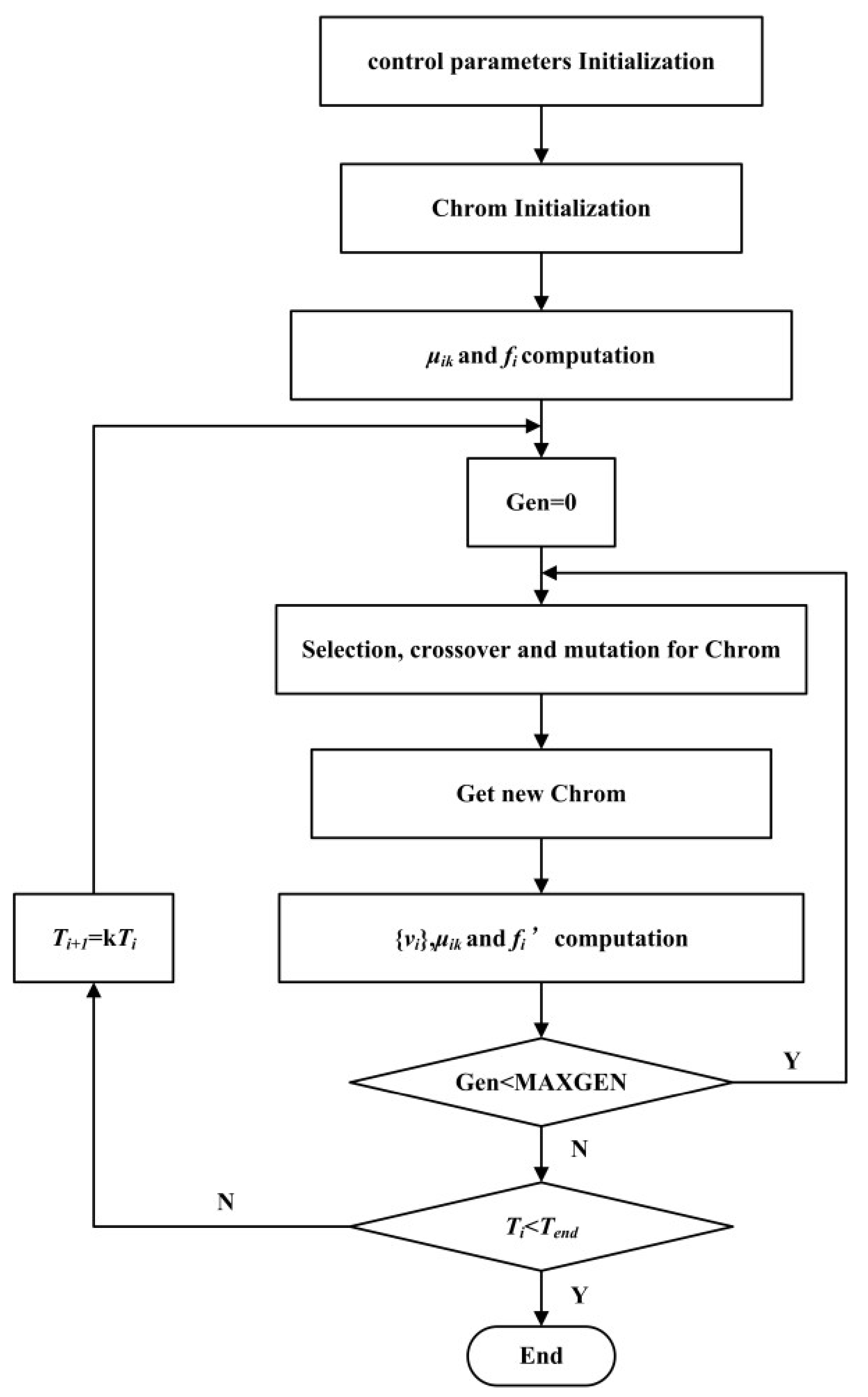
Figure 2.
Flow diagram of LSSVM’s parameters optimization by using Particle Swarm Optimization Algorithm.
Figure 2.
Flow diagram of LSSVM’s parameters optimization by using Particle Swarm Optimization Algorithm.
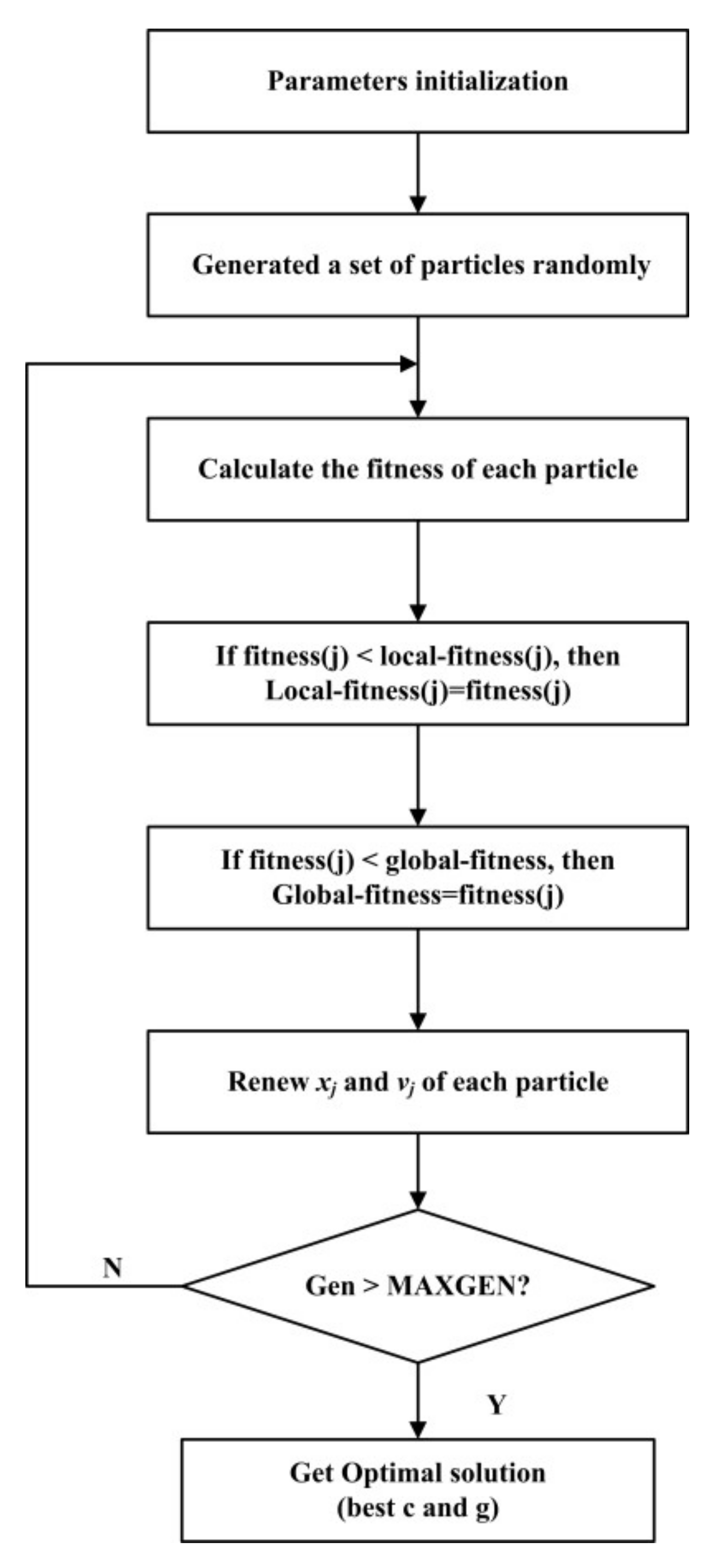
Figure 3.
(a) The location of Ordos Bin in China and (b) the structural belts of Ordos Basin and the sampling well near the Yimeng uplift.
Figure 3.
(a) The location of Ordos Bin in China and (b) the structural belts of Ordos Basin and the sampling well near the Yimeng uplift.
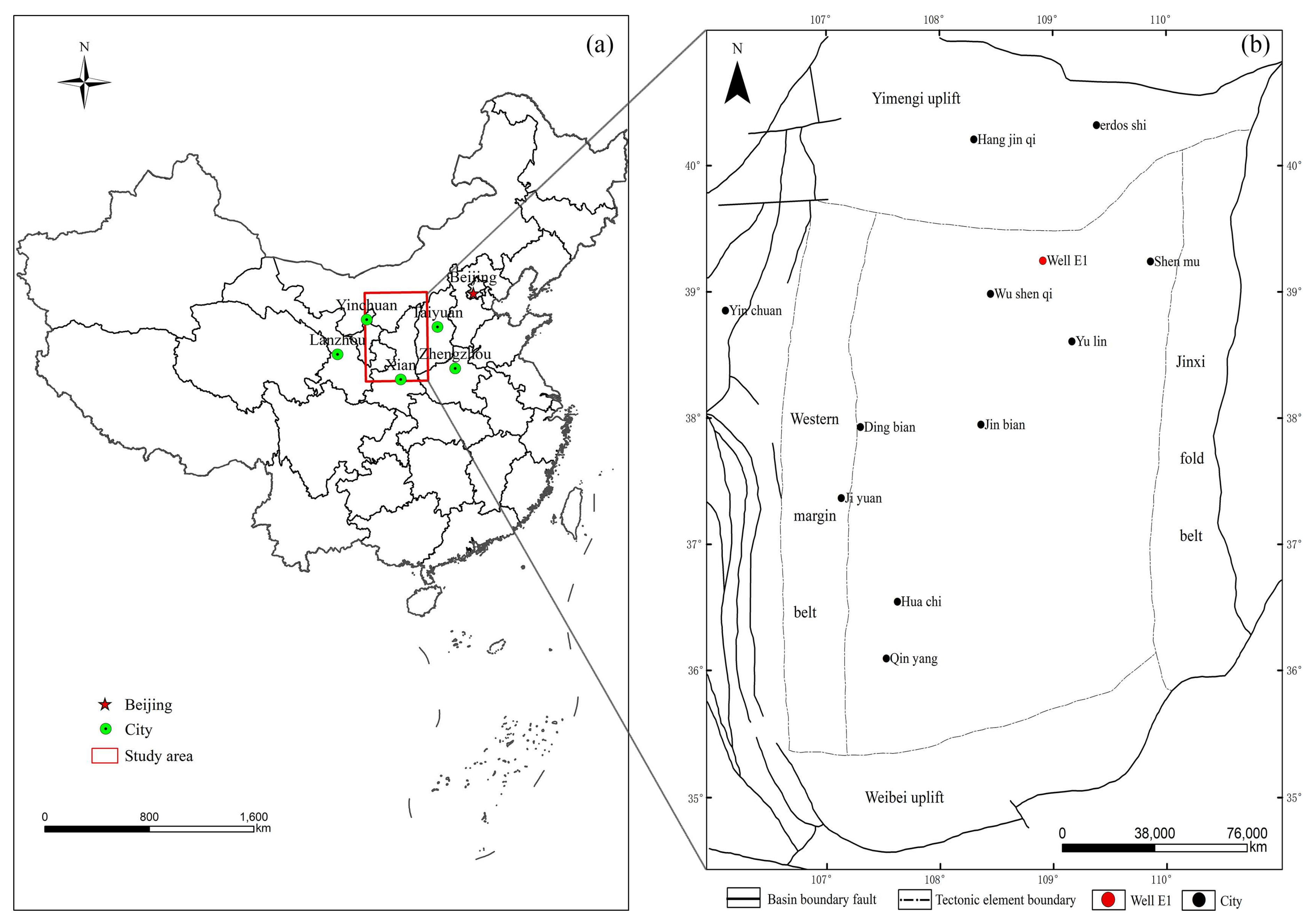
Figure 4.
Cross-plots of TOC laboratory-measurements and logging data for Well E1 (a) SP-TOC, (b) GR-TOC, (c) DTC-TOC, (d) RT-TOC, (e) U-TOC, (f) KTH-TOC, (g) TH-TOC, (h) DEN-TOC, and (i) CNL-TOC; R2 = coefficients of determination; n = number of sample points.
Figure 4.
Cross-plots of TOC laboratory-measurements and logging data for Well E1 (a) SP-TOC, (b) GR-TOC, (c) DTC-TOC, (d) RT-TOC, (e) U-TOC, (f) KTH-TOC, (g) TH-TOC, (h) DEN-TOC, and (i) CNL-TOC; R2 = coefficients of determination; n = number of sample points.

Figure 5.
Change rate scattering of the R2 after sample data optimization.

Figure 6.
Structure and schematic diagram of the back-propagation neural network model used in this study.
Figure 6.
Structure and schematic diagram of the back-propagation neural network model used in this study.

Figure 7.
Comparison of the TOC prediction results with the original samples data and laboratory measured TOC: (a) LSSVM-training results; (b) LSSVM-testing results; (c) PSO-LSSVM-training results; (d) PSO-LSSVM-testing results; (e) BPNN-training results; and (f) BPNN-testing results.
Figure 7.
Comparison of the TOC prediction results with the original samples data and laboratory measured TOC: (a) LSSVM-training results; (b) LSSVM-testing results; (c) PSO-LSSVM-training results; (d) PSO-LSSVM-testing results; (e) BPNN-training results; and (f) BPNN-testing results.
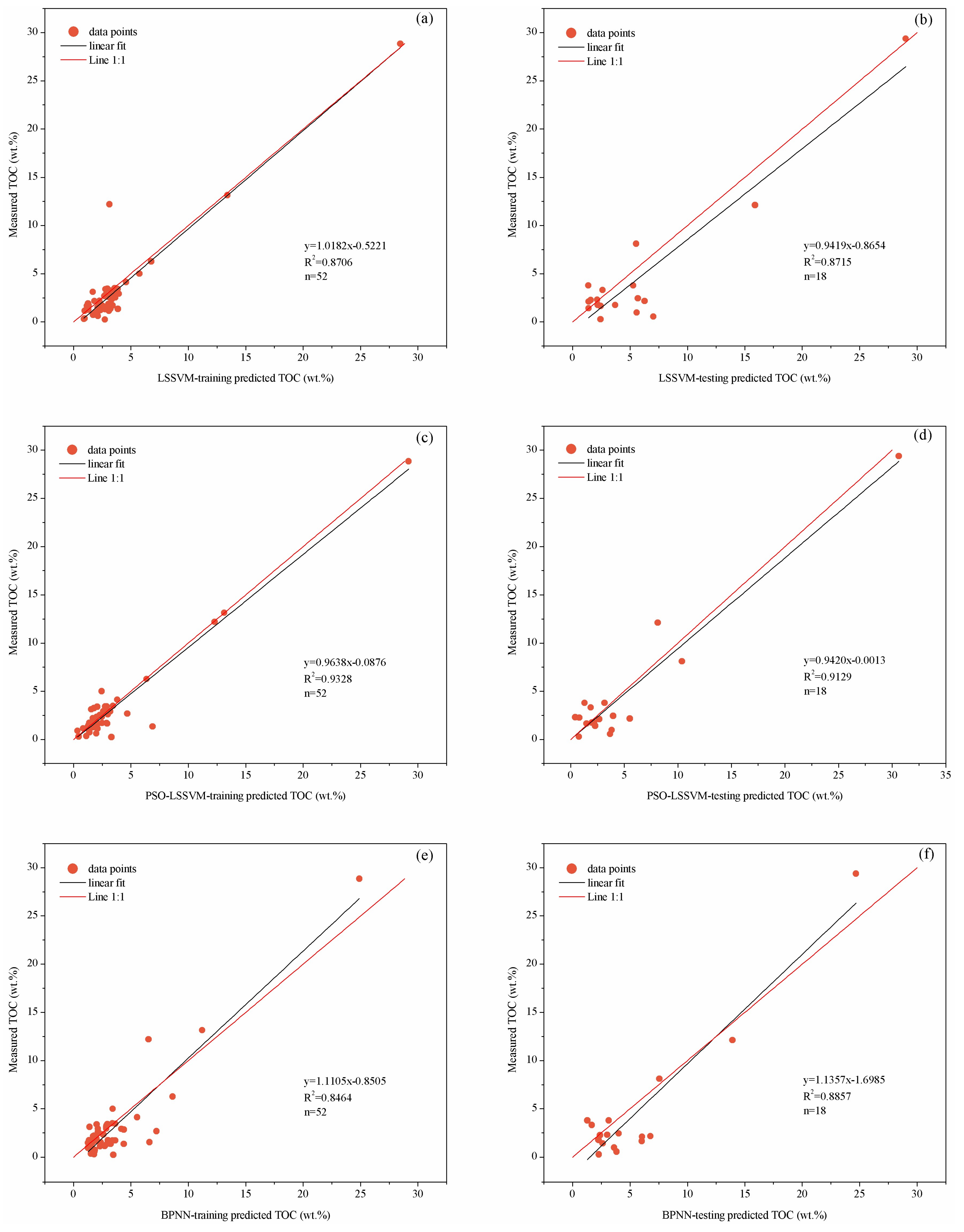
Figure 8.
Comparison of the TOC prediction results with the optimization samples data and laboratory measured TOC: (a) LSSVM-training results; (b) LSSVM-testing results; (c) PSO-LSSVM-training results; (d) PSO-LSSVM-testing results; (e) BPNN-training results; and (f) BPNN-testing results.
Figure 8.
Comparison of the TOC prediction results with the optimization samples data and laboratory measured TOC: (a) LSSVM-training results; (b) LSSVM-testing results; (c) PSO-LSSVM-training results; (d) PSO-LSSVM-testing results; (e) BPNN-training results; and (f) BPNN-testing results.

Figure 9.
Geophysical logging data of Well E1 and the comparison of the TOC prediction results with the prediction models.
Figure 9.
Geophysical logging data of Well E1 and the comparison of the TOC prediction results with the prediction models.
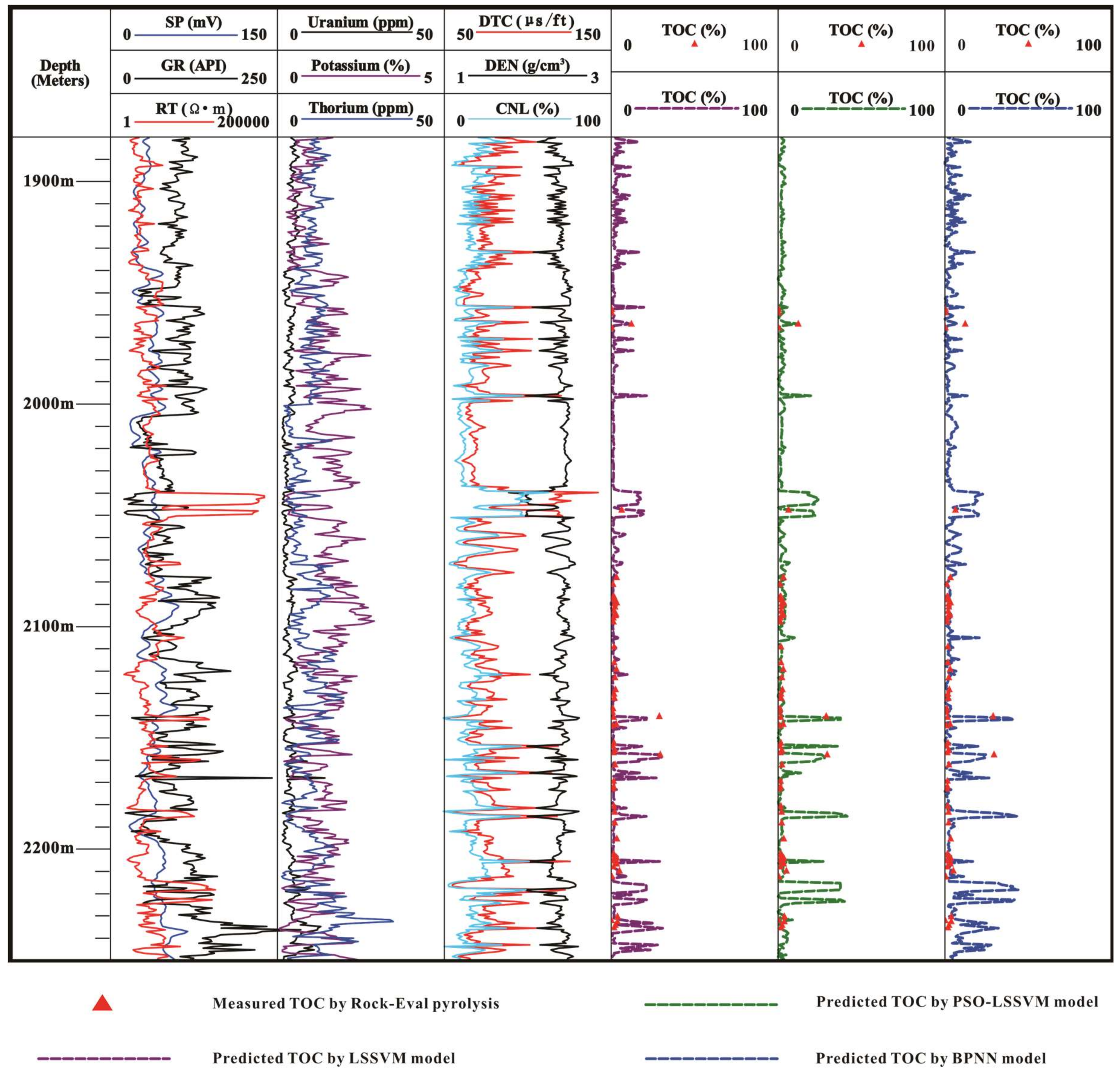
Figure 10.
Image plots showing the graphical comparison between the measured and predicted TOC by the different prediction models. The predicted TOC by PSO-LSSVM model were shown to be extremely consistent with the actual measure TOC in Well E1.
Figure 10.
Image plots showing the graphical comparison between the measured and predicted TOC by the different prediction models. The predicted TOC by PSO-LSSVM model were shown to be extremely consistent with the actual measure TOC in Well E1.

Table 1.
Summary of the recorded logging parameters for Well E1.
| Statistical indicators | Depth (m) | SP (mV) | GR (API) | TDC (μs/ft) | RT (Ω·m) | U (ppm) | KTH (%) | TH (ppm) | DEN (g/cm3) | CNL (%) | TOC (wt.%) |
|---|---|---|---|---|---|---|---|---|---|---|---|
| Miv | 1957.04 | 22.19 | 74.77 | 50.82 | 2.20 | 1.83 | 0.11 | 1.48 | 1.96 | 0.35 | 0.23 |
| Mav | 2234.87 | 63.74 | 196.41 | 128.03 | 89.39 | 7.08 | 2.91 | 21.03 | 2.61 | 34.56 | 29.39 |
| average | 2133.27 | 39.55 | 129.54 | 80.68 | 18.80 | 4.28 | 1.42 | 10.21 | 2.34 | 18.11 | 3.38 |
| SD | 65.92 | 6.42 | 25.09 | 15.38 | 18.76 | 0.99 | 0.70 | 4.83 | 0.12 | 5.85 | 5.09 |
Abbreviations: Miv = Minimum value; Mav = Maximum value; SD = Standard deviation.
Table 2.
Correlation matrix of Well E1.
| Parameters | TOC | SP | GR | DTC | RT | U | KTH | TH | DEN | CNL |
|---|---|---|---|---|---|---|---|---|---|---|
| TOC | 1 | |||||||||
| SP | 0.6093 | 1 | ||||||||
| GR | 0.4253 | 0.332 | 1 | |||||||
| DTC | 0.649 | 0.4729 | 0.3846 | 1 | ||||||
| RT | 0.7124 | 0.5709 | 0.0462 | 0.4623 | 1 | |||||
| U | 0.5165 | 0.5057 | 0.758 | 0.4908 | 0.1883 | 1 | ||||
| KTH | −0.36 | −0.16 | −0.1096 | −0.3937 | −0.3651 | −0.2429 | 1 | |||
| TH | −0.2156 | −0.0807 | 0.0404 | −0.1692 | −0.2885 | 0.068 | −0.1013 | 1 | ||
| DEN | −0.6294 | −0.3362 | −0.3052 | −0.9278 | −0.3895 | −0.4042 | 0.3887 | 0.2266 | 1 | |
| CNL | 0.5771 | 0.3306 | 0.3736 | 0.8782 | 0.2506 | 0.4717 | −0.3028 | −0.1046 | −0.8706 | 1 |
Table 3.
The logical relationship between Well logs and TOC.
| Well Logs | Physical Interpretation |
|---|---|
| Spontaneous potential and resistivity | (1) Due to the fact that the stratum that was rich in organic carbon had a higher degree of mineralization than the surrounding rock, the potential differences resulting from the diffusion and adsorption between the drilling fluid and interlayer water increased. (2) The organic matter contained in the source rock consisted of non-conductive media, and the enrichment of the organic content led to the growth of the resistivity. |
| Natural gamma ray and spectral gamma | (1) The TOC content influenced the logging value of the natural gamma ray because of the source rock’s fine grains, large specific surface areas, and strong adsorption of organic matter into the radioactive elements. (2) The content of the potassium and thorium is associated with clay minerals. So, there is a weak correlation between the well logs of the potassium and thorium and the TOC content. |
| Sonic logs | The organic matter in the source rock with a high acoustic time difference led to the abnormal high value of the acoustic time difference. |
| Density logs | Since solid-state organic matter is characterized by light weight in terms of the surrounding rock, and its density is close to the density of water. Strata with high TOC generally have low density. |
| Compensated neutron logs | The hydrocarbon in the source rocks is rich in hydrogen element, which leads to an abnormally high neutron log value. Thus, the total organic carbon content in the source rock was closely related to the neutron log value. |
Table 4.
Controlling parameters of the SAGA-FCM algorithm.
| Parameters | b | N | D | Sizepop | MAXGEN | Pc | Pm | T0 | k | Tend |
|---|---|---|---|---|---|---|---|---|---|---|
| Value | 2 | 10 | 1 × 10⁻⁶ | 100 | 100 | 0.7 | 0.01 | 100 | 0.8 | 1 |
Table 5.
Matrix of the grade of membership for the samples.
| Sample No. | HQ | PQ | Results | Sample No. | HQ | PQ | Results | Sample No. | HQ | PQ | Results |
|---|---|---|---|---|---|---|---|---|---|---|---|
| 1 | 0.6279 | 0.3721 | Y | 25 | 0.7116 | 0.2884 | Y | 49 | 0.6402 | 0.3598 | Y |
| 2 | 0.5652 | 0.4348 | Y | 26 | 0.4171 | 0.5829 | N | 50 | 0.3595 | 0.6405 | N |
| 3 | 0.5542 | 0.4458 | Y | 27 | 0.6699 | 0.3301 | Y | 51 | 0.6685 | 0.3315 | Y |
| 4 | 0.6654 | 0.3346 | Y | 28 | 0.7314 | 0.2686 | Y | 52 | 0.5602 | 0.4398 | Y |
| 5 | 0.5443 | 0.4557 | Y | 29 | 0.7134 | 0.2866 | Y | 53 | 0.4618 | 0.5382 | N |
| 6 | 0.4225 | 0.5775 | N | 30 | 0.5694 | 0.4306 | Y | 54 | 0.6129 | 0.3871 | Y |
| 7 | 0.7253 | 0.2747 | Y | 31 | 0.6908 | 0.3092 | Y | 55 | 0.6727 | 0.3273 | Y |
| 8 | 0.4237 | 0.5763 | N | 32 | 0.553 | 0.447 | Y | 56 | 0.7801 | 0.2199 | Y |
| 9 | 0.7173 | 0.2827 | Y | 33 | 0.5611 | 0.4389 | Y | 57 | 0.5927 | 0.4073 | Y |
| 10 | 0.3935 | 0.6065 | N | 34 | 0.5249 | 0.4751 | Y | 58 | 0.5529 | 0.4471 | Y |
| 11 | 0.4786 | 0.5214 | N | 35 | 0.719 | 0.281 | Y | 59 | 0.6544 | 0.3456 | Y |
| 12 | 0.3991 | 0.6009 | N | 36 | 0.7561 | 0.2439 | Y | 60 | 0.5819 | 0.4181 | Y |
| 13 | 0.7062 | 0.2938 | Y | 37 | 0.5281 | 0.4719 | Y | 61 | 0.5284 | 0.4716 | Y |
| 14 | 0.709 | 0.291 | Y | 38 | 0.5646 | 0.4354 | Y | 62 | 0.6731 | 0.3269 | Y |
| 15 | 0.6707 | 0.3293 | Y | 39 | 0.5458 | 0.4542 | Y | 63 | 0.5364 | 0.4636 | Y |
| 16 | 0.7056 | 0.2944 | Y | 40 | 0.7183 | 0.2817 | Y | 64 | 0.5743 | 0.4257 | Y |
| 17 | 0.7236 | 0.2764 | Y | 41 | 0.5302 | 0.4698 | Y | 65 | 0.6157 | 0.3843 | Y |
| 18 | 0.6861 | 0.3139 | Y | 42 | 0.6671 | 0.3329 | Y | 66 | 0.681 | 0.319 | Y |
| 19 | 0.7151 | 0.2849 | Y | 43 | 0.6554 | 0.3446 | Y | 67 | 0.6137 | 0.3863 | Y |
| 20 | 0.6742 | 0.3258 | Y | 44 | 0.6618 | 0.3382 | Y | 68 | 0.7294 | 0.2706 | Y |
| 21 | 0.5096 | 0.4904 | Y | 45 | 0.5288 | 0.4712 | Y | 69 | 0.6422 | 0.3578 | Y |
| 22 | 0.4975 | 0.5025 | N | 46 | 0.6303 | 0.3697 | Y | 70 | 0.7155 | 0.2845 | Y |
| 23 | 0.6239 | 0.3761 | Y | 47 | 0.5978 | 0.4022 | Y | ||||
| 24 | 0.5892 | 0.4108 | Y | 48 | 0.6608 | 0.3392 | Y |
Abbreviations: HQ = high-quality; PQ = poor-quality; Y = yes, which means the sample belongs to the high-quality type; N = no, meaning the sample belongs to the poor-quality type.
Table 6.
Correlation matrix of Well E1 with sample data optimization.
| Parameters | TOC | SP | GR | DTC | RT | U | KTH | TH | DEN | CNL |
|---|---|---|---|---|---|---|---|---|---|---|
| TOC | 1 | |||||||||
| SP | 0.6438 | 1 | ||||||||
| GR | 0.5129 | 0.5297 | 1 | |||||||
| DTC | 0.6889 | 0.5065 | 0.6024 | 1 | ||||||
| RT | 0.7672 | 0.6146 | 0.2173 | 0.357 | 1 | |||||
| U | 0.5415 | 0.5791 | 0.7921 | 0.6014 | 0.2458 | 1 | ||||
| KTH | −0.3897 | −0.1801 | −0.0911 | −0.2821 | −0.3394 | −0.2542 | 1 | |||
| TH | −0.1783 | −0.1139 | 0.0806 | −0.0922 | −0.2083 | 0.0199 | −0.0485 | 1 | ||
| DEN | −0.6792 | −0.3814 | −0.4887 | −0.9094 | −0.2744 | −0.5198 | 0.2786 | 0.0939 | 1 | |
| CNL | 0.6094 | 0.3286 | 0.5748 | 0.8819 | 0.1035 | 0.5922 | −0.1976 | −0.1103 | −0.8625 | 1 |
Table 7.
Calculated R2, RMSE, and VAF indicators of the LSSVM, PSO-LSSVM, and BPNN models.
| Data Set | Performance Indicator | LSSVM Model | PSO-LSSVM Model | BPNN Model |
|---|---|---|---|---|
| Original samples data training part | R2 | 0.8706 | 0.9328 | 0.8464 |
| RMSE | 1.6187 | 1.1464 | 1.7964 | |
| VAF | 84.5567 | 93.1765 | 76.3963 | |
| Original samples data testing part | R2 | 0.8715 | 0.9129 | 0.8857 |
| RMSE | 1.6943 | 1.2055 | 2.0593 | |
| VAF | 86.5811 | 91.2362 | 81.5052 | |
| Optimization samples data training part | R2 | 0.9457 | 0.9568 | 0.9307 |
| RMSE | 0.4142 | 0.3125 | 0.5061 | |
| VAF | 94.5206 | 95.6682 | 91.1356 | |
| Optimization samples data testing part | R2 | 0.9427 | 0.9535 | 0.9324 |
| RMSE | 0.4082 | 0.3675 | 0.5177 | |
| VAF | 92.5779 | 94.1615 | 93.1739 |
Table 8.
Calculated R2, RMSE, and VAF indicators of the LSSVM, PSO-LSSVM, and BPNN models.
| Model | R2 | RMSE | VAF |
|---|---|---|---|
| LSSVM | 0.9316 | 0.4094 | 93.4207 |
| PSO-LSSVM | 0.9451 | 0.3383 | 94.1019 |
| BPNN | 0.9184 | 0.5119 | 91.2551 |
© 2018 by the authors. Licensee MDPI, Basel, Switzerland. This article is an open access article distributed under the terms and conditions of the Creative Commons Attribution (CC BY) license (http://creativecommons.org/licenses/by/4.0/).
Share and Cite
MDPI and ACS Style
Wang, P.; Peng, S. A New Scheme to Improve the Performance of Artificial Intelligence Techniques for Estimating Total Organic Carbon from Well Logs. Energies 2018, 11, 747. https://doi.org/10.3390/en11040747
AMA Style
Wang P, Peng S. A New Scheme to Improve the Performance of Artificial Intelligence Techniques for Estimating Total Organic Carbon from Well Logs. Energies. 2018; 11(4):747. https://doi.org/10.3390/en11040747
Chicago/Turabian StyleWang, Pan, and Suping Peng. 2018. "A New Scheme to Improve the Performance of Artificial Intelligence Techniques for Estimating Total Organic Carbon from Well Logs" Energies 11, no. 4: 747. https://doi.org/10.3390/en11040747
Note that from the first issue of 2016, this journal uses article numbers instead of page numbers. See further details here.