Economic Dispatch of the Low-Carbon Green Certificate with Wind Farms Based on Fuzzy Chance Constraints


1
School of Electrical Engineering, Northeast Electric Power University, Jilin 132012, China
2
State Grid Urumqi Power Supply Company, Urumqi 830011, China
3
State Grid Liaocheng Power Supply Company, Liaocheng 252000, China
*
Author to whom correspondence should be addressed.
Energies 2018, 11(4), 943; https://doi.org/10.3390/en11040943
Submission received: 9 March 2018
/
Revised: 29 March 2018
/
Accepted: 4 April 2018
/
Published: 16 April 2018
Abstract
:As the low-carbon economy continues to expand, wind power, as one form of clean energy, promotes the low-carbon power development process. In this paper, a multi-objective environmental economic dispatch (EED) model is proposed considering multiple uncertainties of the system. Carbon trading costs and green certificate trading costs are introduced into the economic costs. Meanwhile, the objective function of pollutant emissions is taken into account in the model, which can further promote the reduction of pollutant emissions in the system scheduling. The output of wind turbines is uncertain and volatile, so it brings new challenges to the power system EED once the large-scale wind power accesses the power grid. For the multiple uncertainties of the system, fuzzy chance-constrained programming is introduced, and the output of the wind turbines and the load are regarded as fuzzy variables. We use the clear equivalence forms to clarify the fuzzy chance constraints. The improved multi-objective standard particle swarm optimization (SPSO) algorithm is used to solve the optimization problem effectively. The feasibility and effectiveness of the proposed model and algorithm are verified by an example of a 10-unit system with two wind farms.
1. Introduction
Compared with the traditional fossil energy, wind power has the advantages of no energy consumption, no emission and no pollution, and its strategic status is gradually increasing as an alternative energy source and even the dominant energy source [1]. At the same time, with the continuous development of renewable energy power generation, wind power as an important driving force to promote the development of the low-carbon economy has attracted more and more attention [2,3].
The traditional power system economic dispatch (ED) model [4,5] takes the minimum total costs of the scheduling cycle as the goal of the ED model of the power system with wind farms, without considering the environmental problems such as carbon emissions. Tian et al. introduced the carbon emission costs in the power grid planning to limit the CO2 emissions of the power generation system and adopted the advanced emission reduction technology unit for priority scheduling [6]. Wang et al. formulated a multi-objective ED problem considering wind penetration and utilized a modified multi-objective particle swarm optimization (PSO) algorithm to solve the ED model [7]. Cui et al. developed a multi-timescale power system operation model integrating both the unit commitment and ED sub-models [8]. However, in [7,8], they did not consider the uncertainty of wind power forecasts, nor the emission of pollutants. Gómez-Lázaro et al. confirmed that multiple Weibull models are more suitable to characterize aggregated wind power data [9]. Hetzer et al. developed a model with wind energy conversion system generators, in which a Weibull probability density function was used to characterize the stochastic wind speed. Both the risk of overestimation and cost of underestimation of available wind power have been considered by introducing reserve cost and penalty cost into the objective function [10]. However, the valve point cost of the thermal power unit is not taken into account in its economic costs. Meibom et al. established the intraday rolling optimization scheduling model on the basis of the wind power probability prediction, and the model was solved quickly by using the method of reduced scene tree [11]. However, the system operation risk is not considered in the model. Azizipanah-Abarghooee et al. developed a new multi-objective stochastic framework based on chance-constrained programming, and this framework benefits from a new method named the hybrid modified cuckoo search (HMCS) algorithm and differential evolution to extract the Pareto-optimal surface for minimum cost and maximum probability of meeting the target cost [12].
Currently, wind power has been developed and utilized in many countries on a larger scale, but large-scale wind power production is variabile [13,14]. Its uncertainty, fluctuation and anti-peaking characteristics [15,16,17,18] cause many problems for wind power access and operation scheduling. Scholars and researchers pay more attention to the study of the uncertainty of wind power [19,20,21], and they have proposed many methods to deal with EED with wind power problems. Jiang et al. established a wind-thermal economic emission dispatch (WTEED) model, where the wind power cost was considered as a part of the optimization objective function. The gravitational acceleration enhanced particle swarm optimization (GAEPSO) algorithm was applied to optimize the costs and emission objectives [22]. Hooshmand et al. proposed a new approach based on a hybrid algorithm consisting of genetic algorithm (GA), pattern search (PS) and sequential quadratic programming (SQP) techniques to solve the well-known power system economic dispatch problem (ED) [23]. Azizipanah-Abarghooee et al. proposed a multi-objective stochastic search algorithm to analyze the probabilistic WTEED problem considering both overestimation and underestimation of available wind power [24]. Morshed et al. formulated and solved a probabilistic optimal power flow approach (POPF) for a hybrid power system. In the proposed approach, the Monte Carlo simulation (MCS) was combined with the antithetic variates method (AVM) to determine the probability distribution function (PDF) of the power generated by the hybrid system [25]. Azizipanah-Abarghooee et al. proposed an improved gradient-based Jaya algorithm to generate a feasible set of Pareto-optimal solutions corresponding to the operation cost and emission calculated through a new robust bi-objective gradient-based method [26]. Morshed et al. proposed a new method based on a hybrid algorithm consisting of the imperialist competitive algorithm (ICA) and the sequential quadratic programming (SQP) technique to solve the power system economic load dispatch (ELD) problem [27]. Alham et al. set a multi-objective optimization model considering the uncertainty of wind power. The multi-objective problem can be transformed into a single-objective optimization problem by the weighted sum method, where the optimal Pareto front is obtained by changing weight factors [28]. The above literature works do not take into account the trading costs of green certificates, and the introduction of green certificate trading costs into scheduling has practical significance along with the promotion of green certificates in various countries [29,30]. Therefore, it is realistic to consider the green certificate transactions in EED.
This paper is organized as follows: Section 2 describes the fuzzy chance-constrained programming. Section 3 and Section 4 set up the green certificate transaction cost model and the carbon transaction cost model, respectively. Section 5 proposes an EED model of the power system with wind farms. Section 6 presents the improved SPSO algorithm for solving the proposed EED model. In Section 7, the results of a 10-unit system with two wind farms are analyzed. Finally, Section 8 summarizes the conclusions.
2. Fuzzy Chance-Constrained Programming
2.1. Clear Equivalence Forms of Fuzzy Chance Constraints
Fuzzy chance-constrained programming is a branch of fuzzy programming, which is used to solve the problem that the constraints contain fuzzy variables. The optimization problem with the constraints containing fuzzy variables can be formulated as:
where x is the decision vector, ξ is the fuzzy parameter vector, f(x) is the objective function and g(x,ξ) is the constraint function.
The existence of fuzzy parameters leads to the constraint condition not being able to give a definite feasible set. Thus, the chance-constrained processing is applied, that is the constraint condition is expected to be set at a certain confidence level of α, that is:
where α is the confidence level; Cr{•} is the probability of the event in {•}.
Clear equivalence forms can deal with the chance-constrained conditions. If the condition of constraint g(x,ξ) is as follows:
where ξk is the trapezoidal fuzzy parameter (rk1, rk2, rk3, rk4), k = 1, 2, …, t, t ∈ R, and rk1–rk4 are the membership parameters.
Define two functions:
where k = 1, 2, …, t. Specially, if h(x) = 1, then h+(x) = 1, h−(x) = 0; if h(x) = −1, then h+(x) = 0, h−(x) = 1.
When the confidence level α ≥ 0.5, the clear equivalence form of the chance constraint (such as Equation (3)) is:
2.2. Membership Function of Fuzzy Parameters
Fuzzy parameter of the load and the output of wind turbines can be represented by a trapezoidal function in the scheduling cycle:
where μ(PF) is a trapezoidal membership function and PFi (i = 1, 2, 3, 4) is the trapezoidal membership parameter.
PFi can be determined based on the predicted value Pforecast:
where ωi (i = 1, 2, 3, 4) is the coefficient of proportionality, 0 < ωi < 1. The coefficient of proportionality can generally be determined by the historical data of the wind turbine output and the load.
The trapezoidal fuzzy parameter can be represented by four tuples:
The trapezoidal fuzzy parameter is shown in Figure 1.
3. Green Certificate Trading Cost Modeling
3.1. Indicator and Production of Green Certificate
The green certificate trading mechanism is put forward on the basis of a renewable energy quota system. At present, this mechanism has been widely used in Britain, the United States, Australia and other countries. In this paper, we define the electric energy produced by the thermal power unit to be non-green electric energy, and the electric energy generated by the wind turbine is green electric energy. Generally, in the scheduling cycle, the system can obtain one green certificate when it produces 1 MWh of green electric energy. According to the total output of the system, the government mandates configuring a certain green electric energy production target. The system will use green electric energy to exchange green certificates and pay the required green certificates before the deadline, otherwise it will face high fines.
Within the unit period of t, the green certificate indicator of the government for the system is:
where Rqt is the green certificate production indicator required by the government within the unit period of t; θ is the proportion coefficient of the green electric energy allocated by the government according to the output of the system; PDt is the sum of the output of wind turbines and thermal power units within the unit period of t, that is , where N is the number of thermal power units, PGit is the output of the thermal power unit i within the unit period of t, NW is the number of wind turbines, PWjt is the output of the wind turbine j within the unit period of t and ε is the amount of the green electric energy needed to exchange a green certificate.
In the power system with wind farms, only the electric energy produced by the wind farm is green electric energy. Within the unit period of t, the amount of the green certificate exchanged by the green electric energy produced by the system is:
where Rpt is the amount of the green certificates exchanged for the green electric energy produced by the system.
3.2. Green Certificate Trading Cost Model
The green certificate trading process in the power system analyzed in this paper has three cases: (1) when the amount of the green certificates exchanged is larger than the amount of the government indicator, the excess green certificates are sold, as well as the proceeds from it; (2) when the amount of the green certificate exchanged is less than the amount of the government indicator, but greater than the difference between the amount of the government indicator and the amount of the green certificate that can be purchased, the cost of the green certificate purchased should be paid; (3) when the amount of the green certificate exchanged is less than the difference between the amount of the government indicator and the amount of the green certificate that can be purchased, in addition to the payment of the purchase cost of the green certificate, also the fine for the amount of the vacancies needs to be paid; that is:
where KRt is the price of the green certificate trading within the unit period of t; KHt is the penalty price of the green certificate of the amount of the vacancies within the unit period of t; RLt is the amount of the green certificate that can be purchased by the system within the unit period of t; ϕ is the margin of the amount of the green certificate that can be purchased; FRt is the green certificate trading costs of the system within the unit period of t; T is the total number of periods of the day-ahead dispatch, taking 24 as the value; FR is the green certificate trading costs of the system in the scheduling cycle T.
4. Carbon Trading Cost Modeling
4.1. Allocation of Carbon Emission Rights and Carbon Emissions
At present, there are mainly two ways to allocate the initial amount of carbon emission rights in the world: one is the free allocation for specific rules; the other is the paid distribution of the auction methods. The paid distribution of the initial carbon emission rights will increase the cost of power generation companies, while the free allocation of the initial carbon emission rights is easy for power generation companies to accept. In this paper, the method of the baseline is used to link the allocation of carbon emission rights and the power generation of the system. Both thermal power units and wind turbines use a distribution method that is proportional to the amount of electricity generated to increase the utilization of clean energy. For a power generation system with wind farms, the amount of carbon emission rights allocated to it within the unit period of t is:
where Eqt is the amount of carbon emission rights allocated by the system within the unit period of t; η is the amount of carbon emissions quota allocated per unit quantity of electricity, determined by the “regional grid baseline emission factor” issued by the China National Development and Reform Commission [31].
Wind power as a green clean energy, the wind farm does produce carbon emissions during the production process. Therefore, in the power system that contains wind farms, carbon emissions are only related to thermal power units. The system carbon emissions within the unit period of t are:
where δi is the carbon emission intensity of the unit quantity of electricity of a thermal power unit I and Ept is the carbon emission of the system within the unit period of t.
4.2. Carbon Trading Costs Model
The carbon trading process in the power system analyzed in this paper has three cases: (1) when the carbon emission is less than the carbon emission rights quota, the excess carbon emission rights quota is sold, as well as the proceeds from it; (2) when the carbon emission is larger than the carbon emission rights quota, but less than the sum of the self-allocation of the carbon emission rights quota and the carbon emission rights that can be purchased, the cost of the carbon emission rights purchased should be paid; (3) when the carbon emission is larger than the sum of the self-allocation of the carbon emission rights quota and the carbon emission rights that can be purchased, in addition to the payment of the purchase cost of carbon emission rights, also the fine of the amount of the excesses needs to be paid. That is:
where KCt is the price of the carbon emission rights trading within the unit period of t; KLt is the penalty price of the carbon emission rights of the amount of the excesses within the unit period of t; ECt is the carbon emission rights that can be purchased by the system within the unit period of t; ρ is the margin of the carbon emission rights that can be purchased; FCt is the carbon trading costs of the system within the unit period of t; FC is the carbon trading costs of the system in the scheduling cycle T.
5. Green Low-Carbon Economic Dispatch Model of the Power System with Wind Farms
5.1. Objective Function of Economic Costs
When considering the carbon trading costs of the system, its economic cost objective function is:
When considering the green certificate trading costs of the system, its economic cost objective function is:
where F1 is the economic cost objective function of the system in the scheduling cycle T; FG is the economic costs of thermal power units’ operation in the scheduling cycle T; FW is the economic costs of wind turbines’ operation in the scheduling cycle T.
The economic costs of the thermal power units FG can be formulated as:
where C(PGit) is the fossil energy consumption cost of the thermal power unit i within the unit period of t; E(PGit) is the energy consumption cost of the valve point effect of the thermal power unit i within the unit period of t; IGit is the operation status of the thermal power unit i within the unit period of t, where IGit = 1 indicates that the unit is in operation, IGit = 0 indicates that the unit is in shutdown; SGit is the start-up cost of the thermal power unit i within the unit period of t.
where ai, bi and ci the generation cost coefficients of the thermal power unit i; ei and fi are the valve point effect coefficients of the thermal power unit i; PGimin is the lower limit of the output of the thermal power unit i; ψi, σi and τi are the start-up cost coefficients of the thermal power unit i; TGitoff is the downtime of the thermal power unit i within the unit period of t.
There is no consumption of fossil energy in the operation of wind turbines. On the basis of considering the cost of wind power investment and operation and maintenance, the average generation cost in the whole life cycle of wind power can be approximately expressed as the linear relationship with the power generation. That is:
where KW is the generation cost coefficient of wind turbines within the unit period of t.
5.2. Objective Function of Pollutant Emissions
During the course of operation, the thermal power generating units not only produce CO2, but also produce pollutants such as sulfur oxides, nitrogen oxides and other polluting gases. These polluting gases will have some influence on the ecological balance (such as fog and haze, acid rain, ozone damage and greenhouse effect) [32]. The objective function of the pollutant emission of the system can be written as:
where F2 is the objective function of system pollutant emission; gi and hi are the weight coefficients of SO2 and NOx emissions of the thermal power unit i; , and are the emission coefficients of SO2 of the thermal power unit i; , and are the emission coefficients of NOx of the thermal power unit i.
5.3. Unit Constraints
Unit output constraint:
Unit ramp rate constraint:
Unit start and stop time constraint:
where PGimax is the upper limit of the output of the thermal power unit i; Rui and Rdi are the ramp-up rate constraint values and the ramp-down rate constraint values of the thermal power unit i, respectively; TGiton is the boot time of the thermal power unit i within the unit period of t; TGiminon and TGiminoff are the minimum boot time and the minimum downtime of the thermal power unit i, respectively.
5.4. System Constraints
5.4.1. System Chance Constraints
When the fuzzy parameters express the output of the wind turbine and load, constraints under certain conditions of the power balance of the system are meaningless. Therefore, the fuzzy chance-constrained programming model is adopted, and its constraints include fuzzy variables. The inequality constraints are established at a certain confidence level and are expressed in the form of probability. The level of confidence can reflect the decision maker’s requirement for the operation level of the power system. The system power balance chance constraint is:
where is the load fuzzy parameter within the unit period of t; is the output fuzzy parameter of the wind turbine j within the unit period of t; α is the confidence level.
Due to the uncertainty of the load and the output of the wind turbine, it is necessary to add reserve power to reduce the risk of the load loss and the risk of the waste of wind energy resource, that is spinning reserve constraints are introduced into the constraints. Reserve is the treatment of the uncertainty of the prediction value. After the fuzzy parameter is used to represent the prediction value, the chance-constrained condition includes the treatment of the uncertainty of the prediction value. Therefore, there is no need to introduce reserve power in the spinning reserve constraint. The spinning reserve chance constraint of the system is:
5.4.2. Clear Equivalence Forms of System Chance Constraints
Using the method of Section 2, the power balance constraint (Equation (32)) and the spinning reserve constraint (Equation (33)) of the system are transformed into the corresponding clear equivalence forms.
The clear equivalence form of the system power balance constraint:
The clear equivalence form of the system spinning reserve constraint:
6. Model Solving
6.1. Pareto Optimal Solution
When there are multiple objective functions, there is usually a bunch of solutions that cannot be simply compared with each other. This solution is called the Pareto-optimal solution or non-dominated solution. The set consisting of all Pareto-optimal solutions is called the Pareto-optimal solution set of the multi-objective optimization problem.
For the multi-objective optimization problem, individual x1 dominates individual x2 (i.e., x1 ≺ x2) if and only if the following relationship is established at the same time:
where fi(x) is the i-th objective function and k is the number of objective functions.
All non-dominated individuals constitute the Pareto-optimal solution S, correspondingly in the target space to form the Pareto optimal leading edge PF
6.2. Improved Multi-Objective Standard Particle Swarm Optimization
In the standard particle swarm optimization (SPSO), the inertia weight ω decreases linearly in the iterative process, so that the PSO algorithm has good global search performance at the beginning, can be quickly positioned near the global optimal point, has good local search performance in the later stage and can accurately get the global optimal solution. Its inertia weight ω is:
where t is the number of iterations; tmax is the maximum number of iterations; ωstart is the initial inertia weight; ωend is the terminal inertia weight.
The biologic heuristic algorithm has a great advantage in solving the optimal problem. Use the predation behavior of birds to improve the SPSO algorithm. Birds not only have predation behavior, but also have anti-predation behavior, that is to say, birds hunt for food while avoiding natural enemies. Then, we set the worst particle in the iteration process, and after each search, the worst particle is obtained by comparison, taking into account the next iteration to update the speed and location. That is to say, in the process of bird flight, there must be a bird closest to the food (the best particle), and there must be a bird closest to the natural enemies (the worst particle). Through the sharing of information, birds are kept close to food and away from natural enemies during flight. In this way, each particle updates its velocity and position (deviates from the worst particle and points to the optimal particle), which is more comprehensive than the SPSO in which the velocity and position (points to the optimal particle) of the particle are updated. This algorithm does not easily fall into the local optimal solution, and it is easier to obtain the global optimal solution. Its flowchart is shown in Figure 2. The particle velocity and position update formula is:
where c1 and c2 are the acceleration coefficients of the particle flying to its own optimal position and flying to the global optimal position, c3 and c4 are the acceleration coefficients of the particle deviating from its own worst position and deviating from the global worst position and r1, r2, r3, r4 are random numbers between zero and one.
7. Example Analysis
7.1. Basic Data and Parameters
Take a regional power grid as an example: the area includes 10 thermal power units and two wind farms, and the scheduling cycle takes 24 h. The parameters of the thermal power unit are shown in Table 1. For all thermal power units, the weight coefficients of SO2 and NOx emissions (gi and hi) are 0.5. The allocation quota of carbon emission per unit of electricity in the system η is 0.798. The green electric energy distribution quota θ is 0.3. The amount of green electric energy needed to exchange a green certificate ε is 1 MWh/copy. The generation cost coefficient of wind turbines KW is 79$/MW. Load prediction is shown in Table 2. The output prediction of two wind farms is shown in Table 3. Load prediction and wind power output prediction are represented by trapezoidal fuzzy parameters, and the values of trapezoidal fuzzy membership parameters are shown in Table 4. The population size of the particles is 20. The maximum number of iterations is 300.
7.2. Calculation Results and Analysis
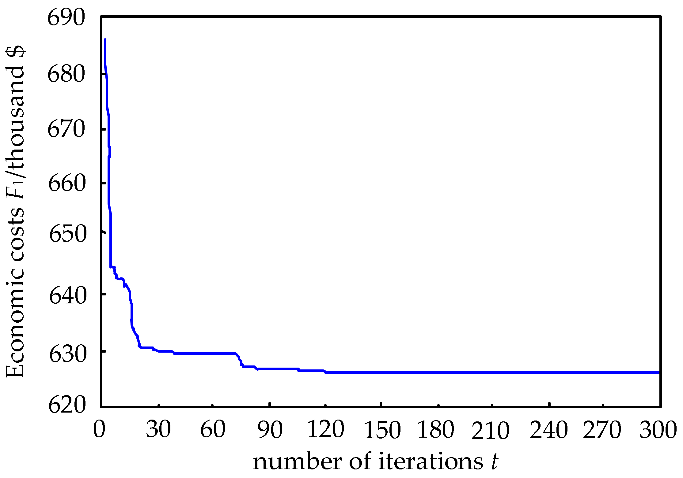
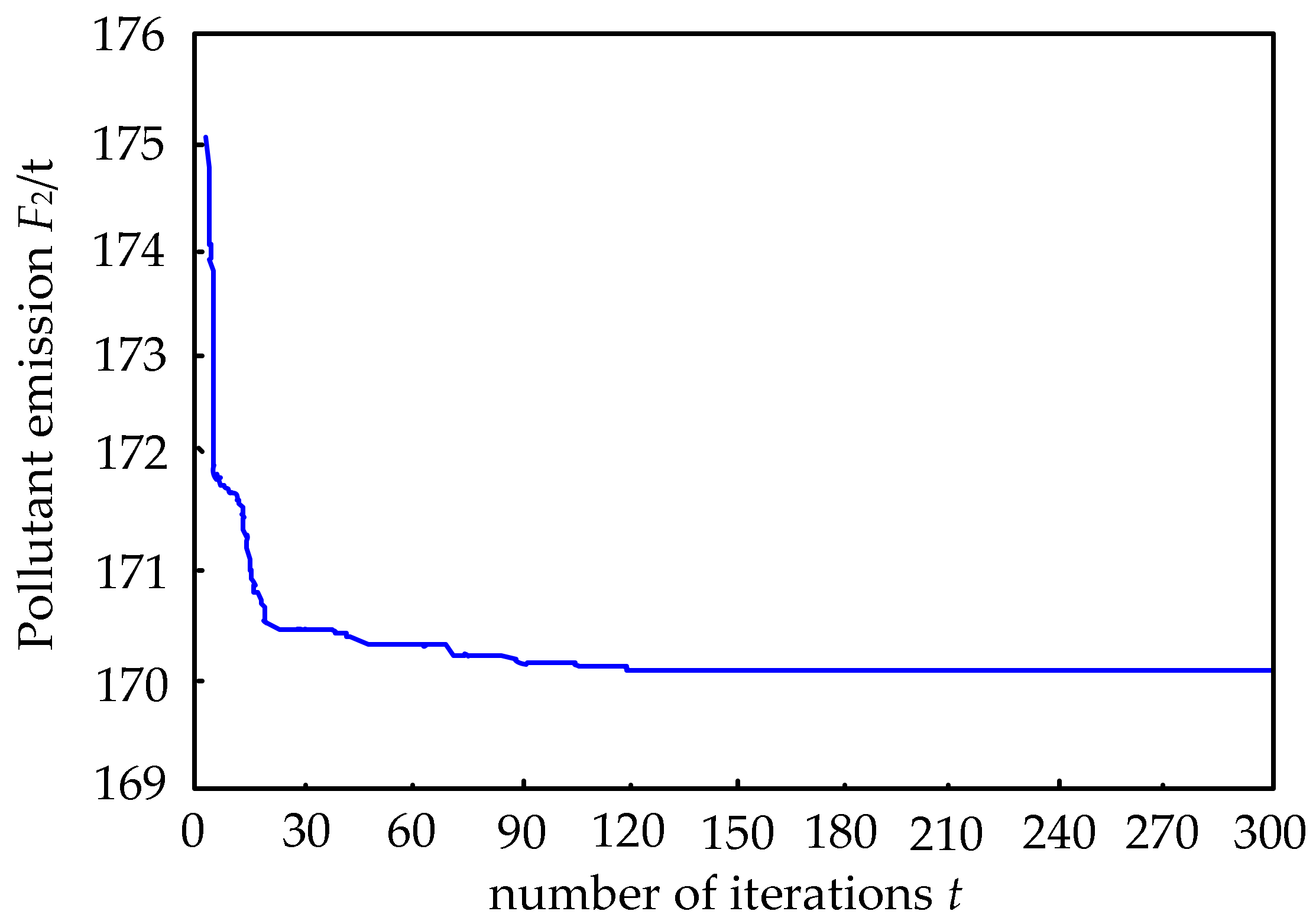
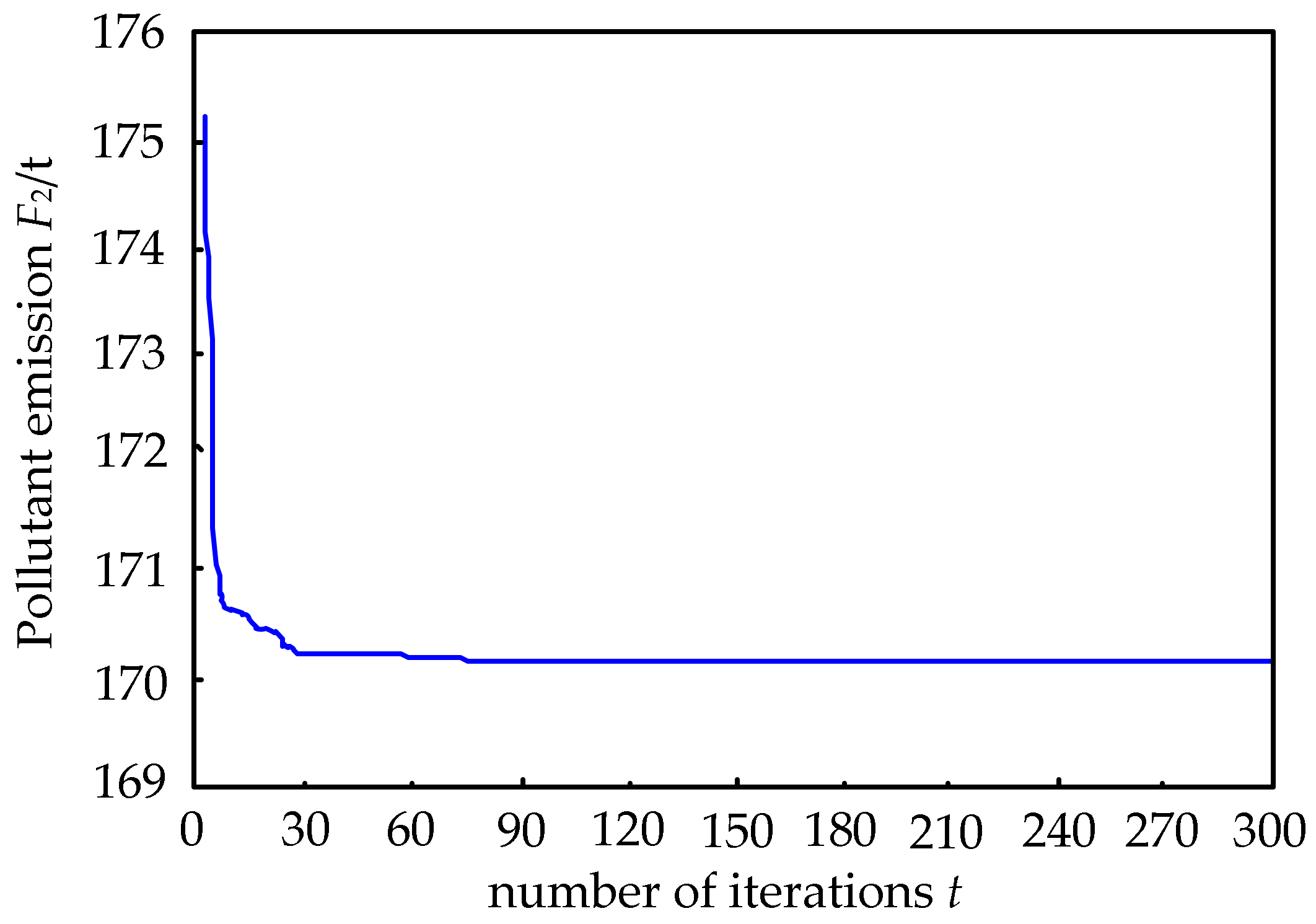
Consider the carbon trading (i.e., the economic costs objective function is Equation (21)). The carbon trading penalty price KLt is 60$/t; the margin of the carbon emission rights that can be purchased ρ is 0.4; the confidence level α is 0.85; the carbon trading price KCt is 20$/t. Figure 3 and Figure 4 show the change curves of the economic costs and pollutant emissions with the number of iterations under the SPSO algorithm, respectively. Figure 5 and Figure 6 show the change curves of the economic costs and pollutant emissions with the number of iterations under the improved SPSO algorithm, respectively. Table 5 shows the final economic costs and pollutant emissions under the SPSO and improved SPSO algorithms.
It can be seen from Figure 3 and Figure 4 that the economic costs and the pollutant emissions are minimized when the number of iterations reaches 90 times under the SPSO algorithm. Figure 5 and Figure 6 show that when the improved SPSO algorithm is used, the convergence speed is improved, and the minimum values have been reached when the number of iterations is 30. It is proven that the improved SPSO algorithm can improve the optimization speed.
It can be seen from Table 5 that the economic cost is 626.194 thousand dollars and the pollutant emission is 170.037 tons under the improved SPSO algorithm. Its optimal dispatch results are reduced compared with the dispatch results of the SPSO algorithm. It is proven that the improved SPSO algorithm can improve the accuracy of optimization.
Consider the carbon trading (i.e., the economic costs objective function is Equation (21)). The carbon trading penalty price KLt is 60$/t; the margin of the carbon emission rights that can be purchased ρ is 0.4; the confidence level α is 0.85. Figure 7 shows the change curve of total economic costs F1 and system pollutant emission F2 with the change of carbon trading price KCt. Figure 8 shows the change curve of carbon trading costs FC with the change of carbon trading price KCt.
It can be seen from Figure 7 that with the increase of the carbon trading price KCt, the low-carbon scheduling target weight increases, and low emission units and wind turbines gradually gain advantages. Low-emission units and wind turbines’ generating costs are higher, so the total economic costs of the system F1 will increase accordingly. With the increase of the carbon trading price, the increase of the output of the wind turbines makes the output of the thermal power units decrease, so the pollutant emissions of the system F2 will decrease accordingly.
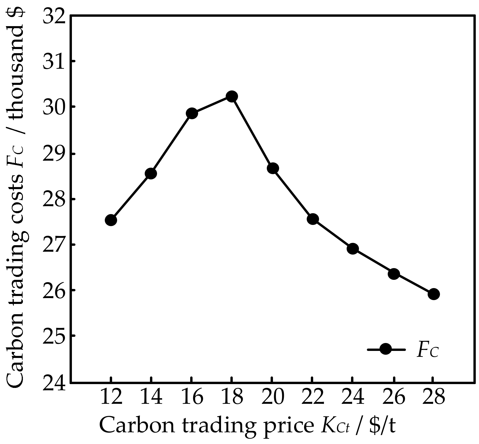
It can be seen from Figure 8 that when the carbon trading price KCt is low, the system of carbon emissions Eqt is greater than the amount of the carbon emission rights quota Eqt. Therefore, it is necessary to purchase carbon emission rights, which results in a certain carbon trading cost FC. With the increase of carbon trading price, the output of wind turbines will increase by a small margin, and the cost of carbon emission rights purchased will increase, so the carbon trading costs will increase. When the carbon trading price reaches 18$/t, the carbon trading costs reach the peak value, which is 30.372 thousand dollars. As the carbon trading price continues to increase, the output of wind turbines will gradually increase, and the system carbon emissions will decrease, so the carbon trading costs decrease. Therefore, the carbon trading costs increase first and then decrease.
Consider the green certificate trading (i.e., the economic costs objective function is Equation (22)). The green certificate trading price KRt is 3$/copy; the green certificate trading penalty price KHt is 9$/copy; the confidence level α is 0.85. Figure 9 shows the change curve of total economic costs F1 and system pollutant emissions F2 with the change of the purchase margin of the green certificate ϕ. Figure 10 shows the change curve of green certificate trading costs FR with the change of the purchase margin of the green certificate ϕ.
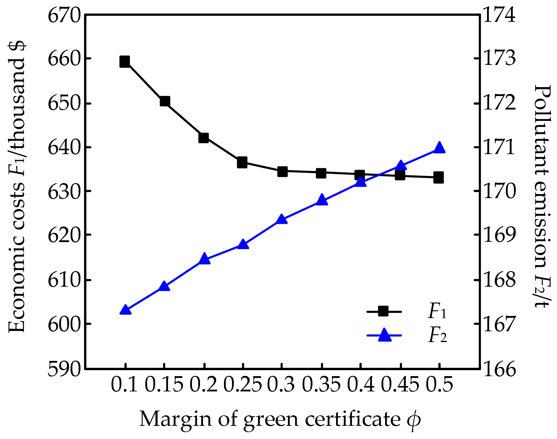
It can be seen from Figure 9 that with the increase of the purchase margin of the green certificate ϕ, the system can purchase more green certificates, so we can reduce the output of high cost low emission units and wind turbines. The total economic costs of the system F1 will decrease accordingly. With the increase of the purchase margin of the green certificate, the decrease of the output of the wind turbines makes the output of the thermal power units increase, so the pollutant emissions of the system F2 will increase accordingly. It can be seen from Figure 7 and Figure 9 that the total economic costs of the system and the emissions of pollutants are restricted by each other, and the relationship between them is negatively related.
It can be seen from Figure 10 that when the green certificate purchase margin ϕ is small, fewer green certificates are purchased, and the cost of green certificate trading FR is the sum of green certificate purchase cost and penalty cost. As the margin of purchase increases, the cost of the green certificate purchased increases, and the cost of the penalty decreases. Because the price of the penalty is higher than the price of green certificate purchased, the trading cost of green certificates is decreasing. As the margin continues to increase, the penalty cost continues to decrease to zero, where the amount of green certificate exchanged Rpt is less than the amount of green certificate quota Rqt, but the amount of green certificate vacancies does not exceed the amount of green certificate that can be purchased RLt, so one only needs to pay the purchase cost of green certificate vacancies. Taking into account that the purchased green certificates can be re-sold, the green certificate trading costs FR have one a small change.
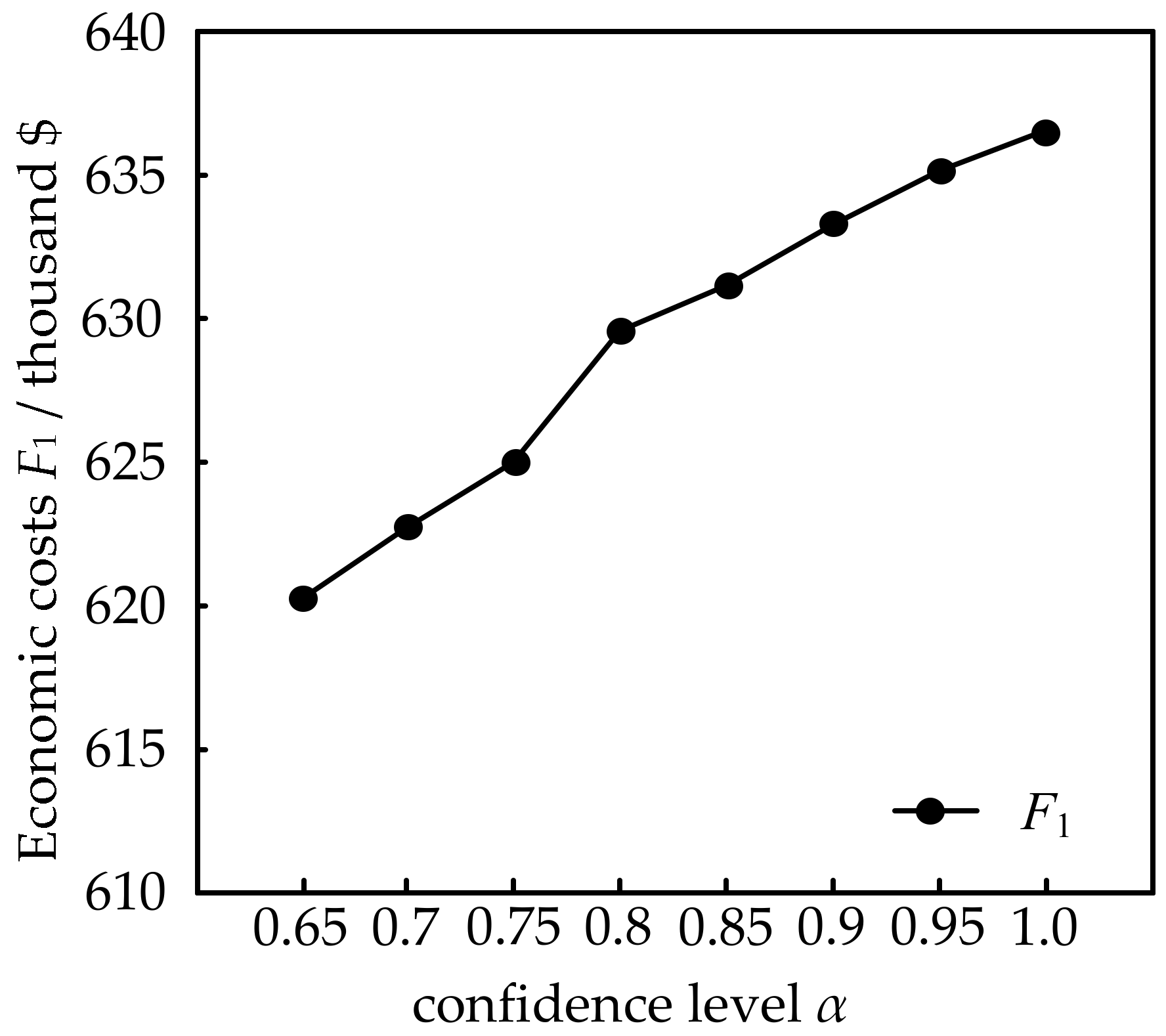
Consider the green certificate trading (i.e., the economic cost objective function is Equation (22)). The green certificate trading price KRt is 3$/copy; the green certificate trading penalty price KHt is 9$/copy; the green certificate purchase margin ϕ is 0.4. Figure 11 shows the change curve of total economic cost F1 with the change of confidence level α.
It can be seen from Figure 11 that when the confidence level α is low, the total economic cost of the system F1 is small, that is to say, high risk brings high returns. With the increase of the confidence level α, the total economic cost of the system F1 is increasing gradually, that is to say, high reliability requires a high cost of investment. The confidence level reflects the decision maker’s grasp of risk, and the risk originates from the fuzziness of load and the output of the wind turbine. In the actual decision making, according to the data analysis of the output of the wind turbine and the load, the unit combination scheme that can accept the above risk and achieve the maximum economic return can be selected.
Consider the green certificate trading (i.e., the economic cost objective function is Equation (22)). The green certificate trading price KRt is 3$/copy; the green certificate trading penalty price KHt is 9$/copy; the green certificate purchase margin ϕ is 0.4; the confidence level α is 0.85. We take the multi-objective economic scheduling in this paper as Model 1. Take the single-objective economic scheduling that only takes the minimum total economic costs of the system F1 as the scheduling goal as Model 2. Take the single-objective economic scheduling that only takes the minimum pollutant emissions of the system F2 as the scheduling goal as Model 3. Table 6 lists the scheduling results in the different models.
It can be seen form Table 6 that under Model 3, only taking the minimum pollutant emissions of the system F2 as the scheduling goal, wind turbines have a priority to generate electricity relative to thermal power units, making the system’s pollutant emissions the smallest. However, due to the high cost of wind power generation, the economic costs of the system are the highest among the three models. Under Model 2, only taking the minimum economic costs of the system F1 as the scheduling goal, thermal power units have a priority to generate electricity relative to wind turbines, making the system’s economic costs the smallest. However, because the thermal power units discharge pollutants while generating electricity, the pollutant emissions of the system are the highest among the three models. The scheduling results of Model 1 are between those of Model 2 and Model 3. This model ensures the system’s scheduling economy, while reducing the amount of pollutant emissions of the system, which is good for environmental protection.
8. Conclusions
This paper presents an EED model of the power system with wind farms. Carbon trading costs and green certificate trading costs are introduced into economic costs. The objective function of system pollutant emission is introduced to further promote the pollutant emission reduction of the system. For the uncertainty and volatility of the load and the output of the wind turbines, this paper regards them as fuzzy variable and establishes the fuzzy chance constraints. The fuzzy chance constraints are clarified by the clear equivalence forms. The optimal allocation of the EED issue involving a 10-unit system with two wind farms is determined by the improved multi-objective SPSO algorithm. Simulation results demonstrate that the algorithm is efficient and the solution is reasonable. The following conclusions can also be reached: (1) The improved SPSO algorithm can improve the optimization speed and the accuracy of optimization relative to the SPSO algorithm in this paper. (2) The total economic costs of the system and the emissions of pollutants are restricted by each other, and the relationship between them is negatively related. (3) Changes of carbon trading price (green certificate trading price) and the purchase margin of the green certificate (purchase margin of carbon emission rights) will produce different influences on the system economic costs and pollutant emissions. Therefore, choosing a reasonable trading price and purchase margin can balance the system economic cost and pollutant emissions. (4) High reliability requires a high cost of investment, while high risk brings high returns. Considering the fuzziness of the load and the output of wind turbines, choosing a reasonable confidence level can realize the control of risks and achieve the minimum economic cost. (5) Relative to single-objective ED, multi-objective EED ensures the system’s scheduling economy, while reducing the amount of pollutant emissions of the system, which is good for environmental protection.
Acknowledgments
This research is funded by the National Natural Science Foundation of China under Grant Number 51777027.
Author Contributions
Xiuyun Wang and Jian Wang conceived of the theory and built the model. Biyuan Tian, Yang Cui and Yu Zhao performed the experiments and analyzed the data. Xiuyun Wang and Jian Wang wrote the paper.
Conflicts of Interest
The authors declare no conflict of interest.
References
- Huo, Y.; Jiang, P.; Zhu, Y.; Feng, S.; Wu, X. Optimal Real-Time Scheduling of Wind Integrated Power System Presented with Storage and Wind Forecast Uncertainties. Energies 2015, 8, 1080–1100. [Google Scholar] [CrossRef]
- D’Amico, G.; Petroni, F.; Prattico, F. Economic Performance Indicators of Wind Energy Based on Wind Speed Stochastic Modeling. Appl. Energy 2015, 154, 290–297. [Google Scholar] [CrossRef]
- Azizipanah-Abarghooee, R.; Golestaneh, F.; Gooi, H.B.; Lin, J.; Bavafa, F.; Terzija, V. Corrective Economic Dispatch and Operational Cycles for Probabilistic Unit Commitment with Demand Response and High Wind Power. Appl. Energy 2016, 182, 634–651. [Google Scholar] [CrossRef]
- Misraji, J.; Conejo, A.J.; Morales, J.M. Reserve-Constrained Economic Dispatch: Cost and Payment Allocations. Electr. Power Syst. Res. 2008, 78, 919–925. [Google Scholar] [CrossRef]
- Park, J.B.; Lee, K.S.; Shin, J.R.; Lee, K.S. A Particle Swarm Optimization for Economic Dispatch with Nonsmooth Cost Functions. IEEE Trans. Power Syst. 2005, 20, 34–42. [Google Scholar] [CrossRef]
- Tian, K.; Qiu, L.; Zeng, M. Method of Grid Planning Based on Dynamic Carbon Emission Price. Proc. CSEE 2012, 32, 57–64. [Google Scholar]
- Wang, L.; Singh, C. Balancing Risk and Cost in Fuzzy Economic Dispatch Including Wind Power Penetration Based on Particle Swarm Optimization. Electr. Power Syst. Res. 2008, 78, 1361–1368. [Google Scholar] [CrossRef]
- Cui, M.; Zhang, J.; Wu, H.; Hodge, B.M. Wind-friendly Flexible Ramping Product Design in Multi-Timescale Power System Operations. IEEE Trans. Sustain. Energy 2017, 8, 1064–1075. [Google Scholar] [CrossRef]
- Gómez-Lázaro, E.; Bueso, M.C.; Kessler, M.; Martín-Martínez, S.; Zhang, J.; Hodge, B.M.; Molina-García, A. Probability Density Function Characterization for Aggregated Large-Scale Wind Power Based on Weibull Mixtures. Energies 2016, 9, 91. [Google Scholar] [CrossRef]
- Hetzer, J.; Yu, D.C.; Bhattarai, K. An Economic Dispatch Model Incorporating Wind Power. IEEE Trans. Energy Convers. 2008, 23, 603–611. [Google Scholar] [CrossRef]
- Meibom, P.; Barth, R.; Hasche, B.; Brand, H.; Weber, C.; O’Malley, M. Stochastic Optimization Model to Study The Operational Impacts of High Wind Penetrations in Ireland. IEEE Trans. Power Syst. 2011, 26, 1367–1379. [Google Scholar] [CrossRef]
- Azizipanah-Abarghooee, R.; Niknam, T.; Bina, M.A.; Zare, M. Coordination of Combined Heat and Power-Thermal-Wind-Photovoltaic Units in Economic Load Dispatch Using Chance-Constrained and Jointly Distributed Random Variables Methods. Energy 2014, 79, 50–67. [Google Scholar] [CrossRef]
- Kiviluoma, J.; Holttinen, H.; Weir, D.; Scharff, R.; Söder, L.; Menemenlis, N.; Cutululis, N.A.; Lopez, I.D.; Lannoye, E.; Estanqueiro, A.; et al. Variability in Large-Scale Wind Power Generation. Wind Energy 2016, 19, 1649–1665. [Google Scholar] [CrossRef]
- Holttinen, H.; Kiviluoma, J.; Estanqueiro, A.; Gómez-Lázaro, E.; Rawn, B.; Dobschinski, J.; Meibom, P.; Lannoye, E.; Aigner, T.; Wang, Y.H.; et al. Variability of Load and Net Load in Case of Large Scale Distributed Wind Power. IEEE Trans. Sustain. Energy 2010, 3, 853–861. [Google Scholar]
- Hodge, B.M.; Holttinen, H.; Sillanpää, S.; Gómez-Lázaro, E.; Scharff, R.; Larsen, X.G.; Giebel, G.; Flynn, D.; Lew, D.; Milligan, M. Wind Power Forecasting Error Distributions: An International Comparison. In Proceedings of the International Workshop on Large-Scale Integration of Wind Power into Power Systems as well as on Transmission Networks for Offshore Wind Farms, Lisbon, Portugal, 13–15 November 2012; Energynautics GmbH: Darmstadt, Germany, 2012; pp. 1–7. [Google Scholar]
- Gautam, D.; Goel, L.; Ayyanar, R.; Vittal, V.; Harbour, T. Control Strategy to Mitigate the Impact of Reduced Inertia Due to Doubly Fed Induction Generators on Large Power Systems. IEEE Trans. Power Syst. 2011, 26, 214–224. [Google Scholar] [CrossRef]
- Tewari, S.; Geyer, C.J.; Mohan, N. A Statistical Model for Wind Power Forecast Error and Its Application to the Estimation of Penalties in Liberalized Markets. IEEE Trans. Power Syst. 2011, 26, 2031–2039. [Google Scholar] [CrossRef]
- Pinson, P.; Kariniotakis, G. Conditional Prediction Intervals of Wind Power Generation. IEEE Trans. Power Syst. 2010, 25, 1845–1856. [Google Scholar] [CrossRef] [Green Version]
- Soroudi, A.; Rabiee, A.; Keane, A. Information Gap Decision Theory Approach to Deal with Wind Power Uncertainty in Unit Commitment. Electr. Power Syst. Res. 2017, 145, 137–148. [Google Scholar] [CrossRef]
- Sharifzadeh, H.; Amjady, N.; Zareipour, H. Multi-Period Stochastic Security-Constrained OPF Considering the Uncertainty Sources of Wind Power, Load Demand and Equipment Unavailability. Electr. Power Syst. Res. 2017, 146, 33–42. [Google Scholar] [CrossRef]
- Ummels, B.; Gibescu, C.M.; Pelgrum, E.; Kling, W.L.; Brand, A.J. Impacts of Wind Power on Thermal Generation Unit Commitment and Dispatch. IEEE Trans. Energy Convers. 2007, 22, 44–51. [Google Scholar] [CrossRef]
- Jiang, S.; Ji, Z.; Wang, Y. A Novel Gravitational Acceleration Enhanced Particle Swarm Optimization Algorithm for Wind–Thermal Economic Emission Dispatch Problem Considering Wind Power Availability. Int. J. Electr. Power Energy Syst. 2015, 73, 1035–1050. [Google Scholar] [CrossRef]
- Hooshmand, R.A.; Parastegari, M.; Morshed, M.J. Emission, Reserve and Economic Load Dispatch Problem with Non-Smooth and Non-Convex Cost Functions Using The Hybrid Bacterial Foraging-Nelder–Mead Algorithm. Appl. Energy 2012, 89, 443–453. [Google Scholar] [CrossRef]
- Azizipanah-Abarghooee, R.; Niknam, T.; Roosta, A.; Malekpour, A.R.; Zare, M. Probabilistic Multiobjective Wind-Thermal Economic Emission Dispatch Based on Point Estimated Method. Energy 2012, 37, 322–335. [Google Scholar] [CrossRef]
- Morshed, M.J.; Hmida, J.B.; Fekih, A. A Probabilistic Multi-Objective Approach for Power Flow Optimization in Hybrid Wind-PV-PEV Systems. Appl. Energy 2018, 211, 1136–1149. [Google Scholar] [CrossRef]
- Azizipanah-Abarghooee, R.; Dehghanian, P.; Terzija, V. Practical Multi-Area Bi-Objective Environmental Economic Dispatch Equipped with A Hybrid Gradient Search Method and Improved Jaya Algorithm. IET Gener. Transm. Distrib. 2016, 10, 3580–3596. [Google Scholar] [CrossRef]
- Morshed, M.J.; Asgharpour, A. Hybrid Imperialist Competitive-Sequential Quadratic Programming (HIC-SQP) Algorithm for Solving Economic Load Dispatch with Incorporating Stochastic Wind Power: A Comparative Study on Heuristic Optimization Techniques. Energy Convers. Manag. 2014, 84, 30–40. [Google Scholar] [CrossRef]
- Alham, M.H.; Elshahed, M.; Ibrahim, D.K.; Zahab, E.E.D.A.E. A Dynamic Economic Emission Dispatch Considering Wind Power Uncertainty Incorporating Energy Storage System and Demand Side Management. Renew. Energy 2016, 96, 800–811. [Google Scholar] [CrossRef]
- Morthorst, P.E. The Development of a Green Certificate Market. Energy Policy 2000, 28, 1085–1094. [Google Scholar] [CrossRef]
- Amundsen, E.S.; Mortensen, J.B. The Danish Green Certificate System: Some Simple Analytical Results. Energy Econ. 2001, 23, 489–509. [Google Scholar] [CrossRef]
- Department of Climate Change, People’s Republic of China National Development and Reform Commission. Public Announcement of Public Opinion on “Emission Factor of China’s Regional Power Grid Baseline in 2016 (Draft for Advice)”. Available online: http://qhs.ndrc.gov.cn/gzdt/201704/t20170414_844347.html (accessed on 14 April 2017).
- Abido, M.A. Multiobjective Evolutionary Algorithms for Electric Power Dispatch Problem. IEEE Trans. Evolut. Comput. 2006, 10, 315–329. [Google Scholar] [CrossRef]
Figure 1.
Trapezoidal fuzzy parameters.
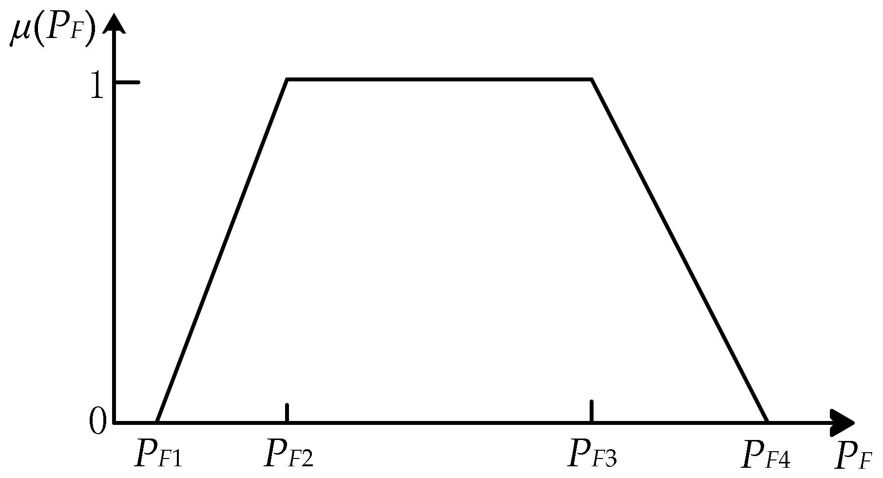
Figure 2.
Flowchart for improved SPSO.
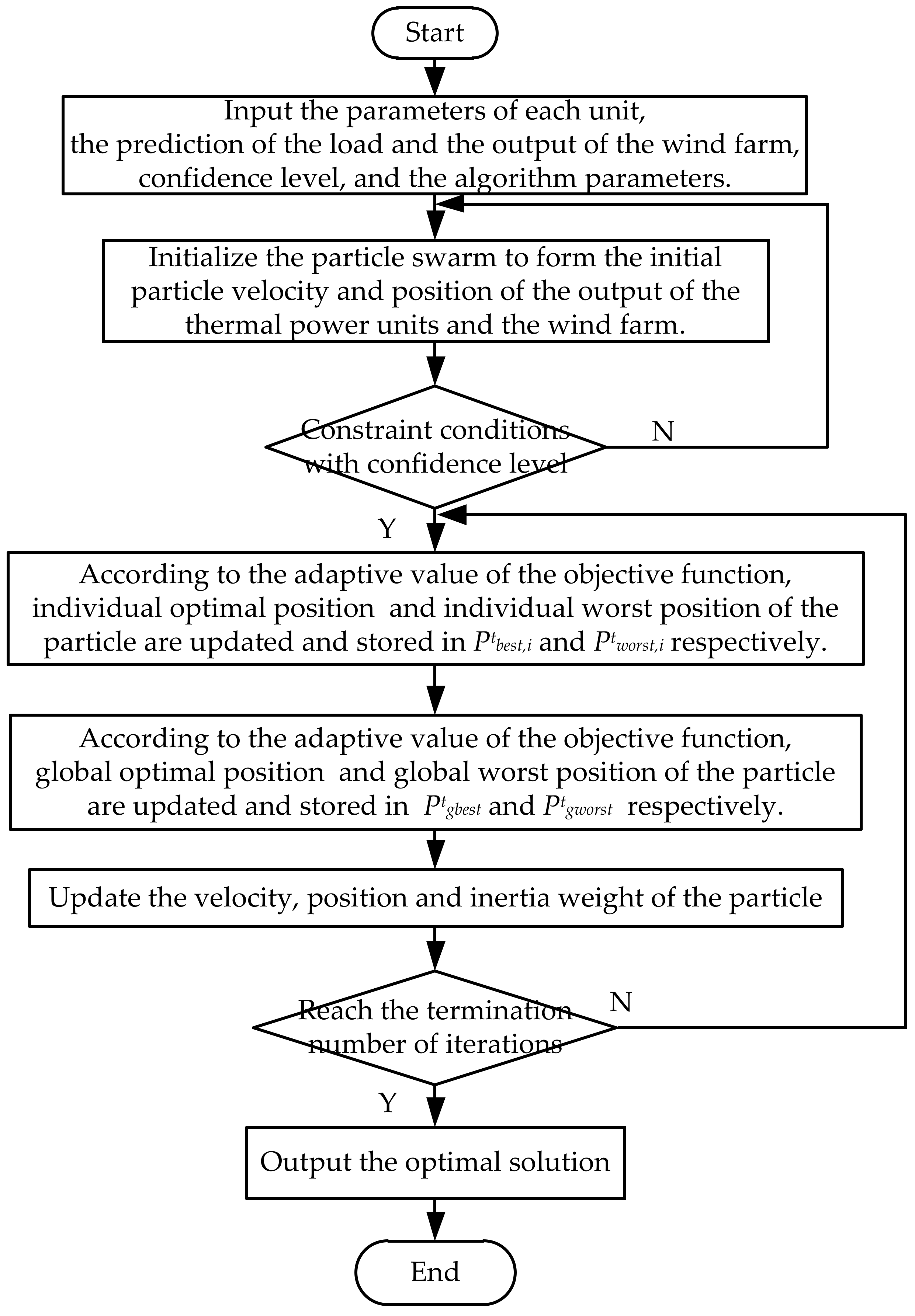
Figure 3.
The change curve of economic costs with the number of iterations (SPSO).

Figure 4.
The change curve of pollutant emissions with the number of iterations (SPSO).

Figure 5.
The change curve of economic costs with the number of iterations (improved SPSO).
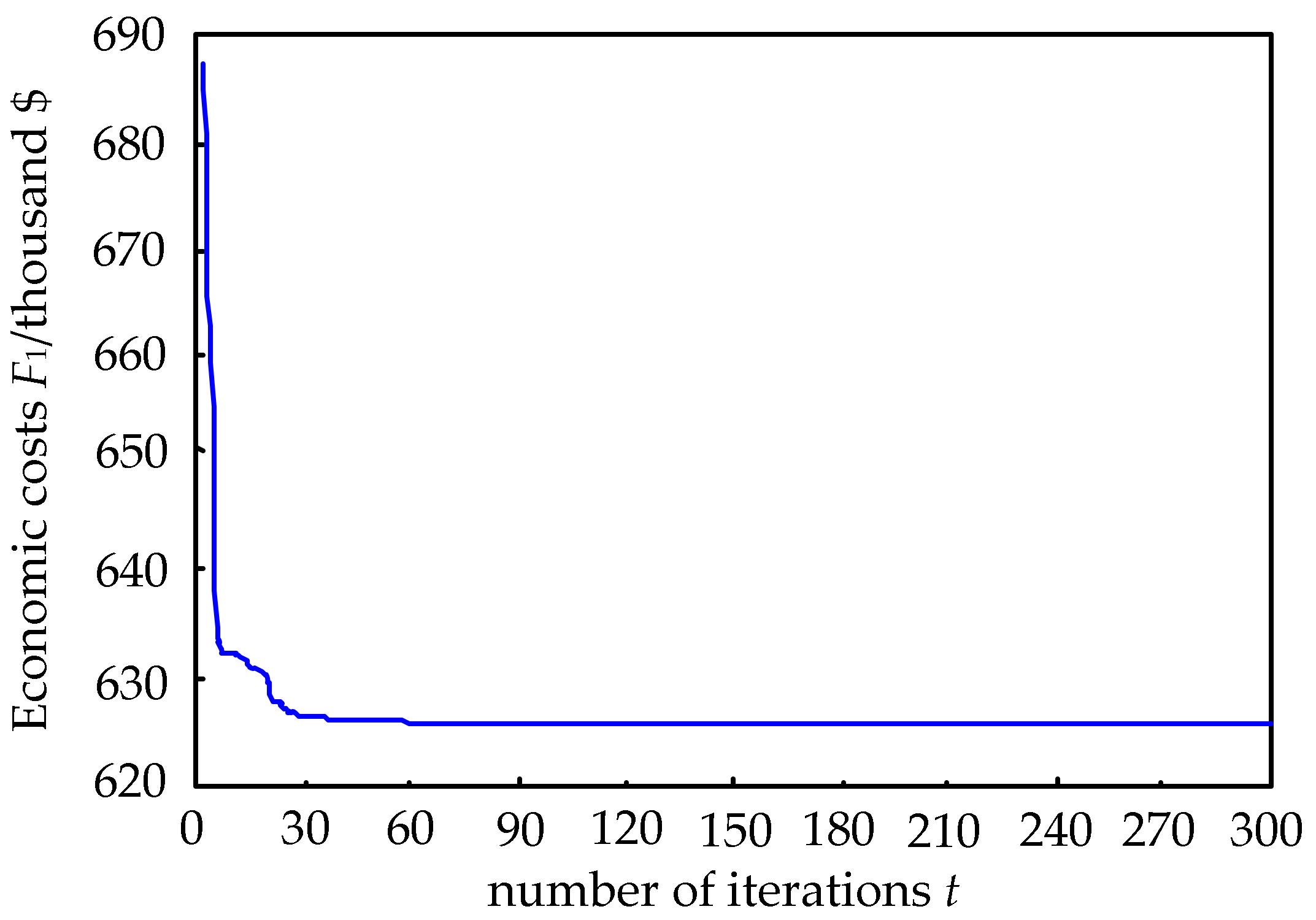
Figure 6.
The change curve of pollutant emissions with the number of iterations (improved SPSO).

Figure 7.
Economic costs and pollutant emission at different carbon trading prices.
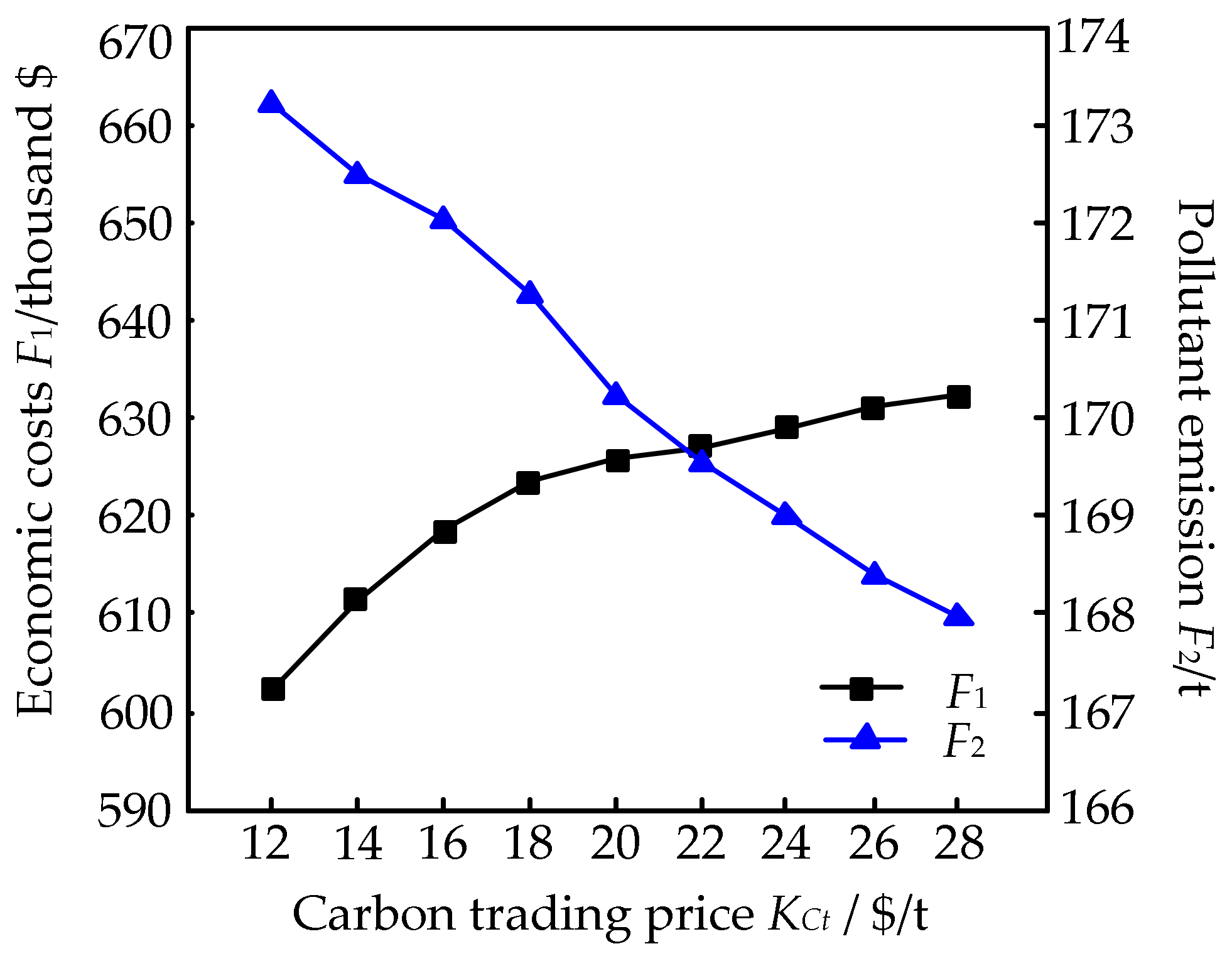
Figure 8.
Carbon trading costs at different carbon trading prices.

Figure 9.
Economic costs and pollutant emission at different margins of the green certificate.

Figure 10.
Green certificate trading costs at different margins of the green certificate.
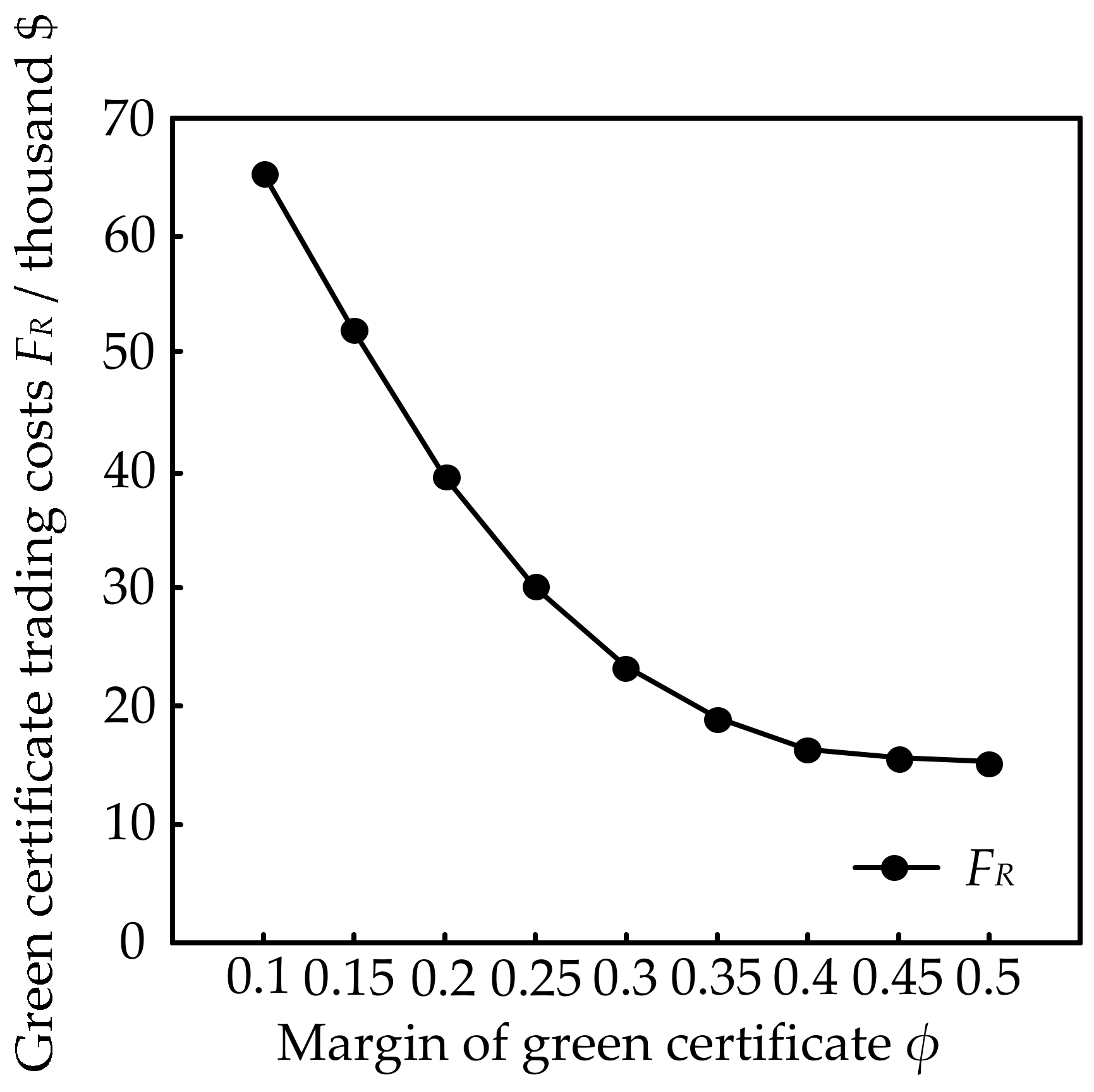
Figure 11.
Economic costs at different confidence levels.


Table 1.
(a) Parameters of the thermal power unit. (b) Parameters of the thermal power unit.
| (a) | ||||||||||
| Unit | Rui/MW/h | Rdi/MW/h | δi | Pmax/MW | Pmin/MW | ai/$/(MW2∙h) | bi/$/(MW∙h) | ci/$/h | ei/$/h | fi/rad/MW |
| 1 | 130 | 130 | 0.97 | 455 | 150 | 0.00048 | 16.19 | 1000 | 450 | 0.041 |
| 2 | 130 | 130 | 0.98 | 455 | 150 | 0.00031 | 17.26 | 970 | 600 | 0.036 |
| 3 | 60 | 60 | 0.98 | 130 | 20 | 0.00200 | 16.60 | 700 | 300 | 0.086 |
| 4 | 90 | 90 | 1.25 | 130 | 20 | 0.00211 | 16.50 | 680 | 340 | 0.082 |
| 5 | 40 | 40 | 1.13 | 162 | 25 | 0.00398 | 19.70 | 450 | 310 | 0.048 |
| 6 | 40 | 40 | 1.22 | 80 | 20 | 0.00712 | 22.26 | 370 | 270 | 0.098 |
| 7 | 40 | 40 | 0.85 | 85 | 25 | 0.00079 | 27.74 | 480 | 300 | 0.092 |
| 8 | 40 | 40 | 0.74 | 55 | 10 | 0.00413 | 25.92 | 660 | 380 | 0.094 |
| 9 | 40 | 40 | 0.74 | 55 | 10 | 0.00222 | 27.27 | 665 | 300 | 0.085 |
| 10 | 40 | 40 | 0.69 | 55 | 10 | 0.00173 | 27.79 | 670 | 290 | 0.078 |
| (b) | ||||||||||
| Unit | aiSO2/kg/(MW2∙h) | biSO2/kg/(MW∙h) | ciSO2/kg/h | aiNOx/kg/(MW2∙h) | biNOx/kg/(MW∙h) | ciNOx/kg/h | ψi/$/h | σi/$/h | τi/h | |
| 1 | 0.00019 | 2.06 | 198.33 | 0.022 | −2.86 | 130.00 | 5500 | 5500 | 5 | |
| 2 | 0.00018 | 2.09 | 195.34 | 0.020 | −2.72 | 132.00 | 5500 | 5500 | 5 | |
| 3 | 0.00220 | 2.14 | 155.15 | 0.044 | −2.94 | 137.70 | 550 | 550 | 2 | |
| 4 | 0.00220 | 2.25 | 152.26 | 0.058 | −2.35 | 130.00 | 550 | 550 | 2 | |
| 5 | 0.00210 | 2.11 | 152.26 | 0.065 | −2.36 | 125.00 | 700 | 700 | 2 | |
| 6 | 0.00250 | 3.45 | 101.43 | 0.080 | −2.28 | 110.00 | 170 | 170 | 2 | |
| 7 | 0.00220 | 2.62 | 111.87 | 0.075 | −2.36 | 135.00 | 200 | 200 | 2 | |
| 8 | 0.00420 | 5.18 | 126.62 | 0.082 | −1.29 | 157.00 | 30 | 30 | 1 | |
| 9 | 0.00540 | 5.38 | 134.15 | 0.090 | −1.14 | 160.00 | 30 | 30 | 1 | |
| 10 | 0.00550 | 5.40 | 142.26 | 0.084 | −2.14 | 137.70 | 30 | 30 | 1 | |
Table 2.
Load prediction for 24 h.
| Hour | Load/MW | Hour | Load/MW | Hour | Load/MW |
|---|---|---|---|---|---|
| 1 | 700 | 9 | 1300 | 17 | 1000 |
| 2 | 750 | 10 | 1400 | 18 | 1100 |
| 3 | 850 | 11 | 1450 | 19 | 1200 |
| 4 | 950 | 12 | 1500 | 20 | 1400 |
| 5 | 1000 | 13 | 1400 | 21 | 1300 |
| 6 | 1100 | 14 | 1300 | 22 | 1100 |
| 7 | 1150 | 15 | 1200 | 23 | 900 |
| 8 | 1200 | 16 | 1050 | 24 | 800 |
Table 3.
Output prediction of two wind farms for 24 h.
| Hour | Wind Farm 1/MW | Wind Farm 2/MW | Hour | Wind Farm 1/MW | Wind Farm 2/MW |
|---|---|---|---|---|---|
| 1 | 190 | 165 | 13 | 390 | 50 |
| 2 | 300 | 145 | 14 | 340 | 115 |
| 3 | 330 | 120 | 15 | 320 | 125 |
| 4 | 360 | 160 | 16 | 120 | 170 |
| 5 | 350 | 140 | 17 | 10 | 150 |
| 6 | 370 | 120 | 18 | 40 | 195 |
| 7 | 440 | 130 | 19 | 50 | 140 |
| 8 | 460 | 80 | 20 | 20 | 240 |
| 9 | 350 | 35 | 21 | 5 | 140 |
| 10 | 250 | 10 | 22 | 250 | 70 |
| 11 | 420 | 75 | 23 | 350 | 10 |
| 12 | 380 | 85 | 24 | 240 | 80 |
Table 4.
Trapezoidal fuzzy membership parameters.
| Fuzzy Parameter | Wind Power Output | Load |
|---|---|---|
| ω1 | 0.6 | 0.9 |
| ω2 | 0.9 | 0.95 |
| ω3 | 1.1 | 1.05 |
| ω4 | 1.4 | 1.1 |
Table 5.
The final F1 and F2 under the SPSO and improved SPSO.
| SPSO | Improved SPSO | |
|---|---|---|
| economic costs F1/k$ | 626.381 | 626.194 |
| pollutant emissions F2/t | 170.105 | 170.037 |
Table 6.
Output prediction of two wind farms for 24 h.
| Model | Economic Costs of the System F1/k$ | Pollutant Emissions of the System F2/t |
|---|---|---|
| 1 | 632.528 | 170.367 |
| 2 | 614.296 | 193.727 |
| 3 | 648.105 | 163.448 |
© 2018 by the authors. Licensee MDPI, Basel, Switzerland. This article is an open access article distributed under the terms and conditions of the Creative Commons Attribution (CC BY) license (http://creativecommons.org/licenses/by/4.0/).
Share and Cite
MDPI and ACS Style
Wang, X.; Wang, J.; Tian, B.; Cui, Y.; Zhao, Y. Economic Dispatch of the Low-Carbon Green Certificate with Wind Farms Based on Fuzzy Chance Constraints. Energies 2018, 11, 943. https://doi.org/10.3390/en11040943
AMA Style
Wang X, Wang J, Tian B, Cui Y, Zhao Y. Economic Dispatch of the Low-Carbon Green Certificate with Wind Farms Based on Fuzzy Chance Constraints. Energies. 2018; 11(4):943. https://doi.org/10.3390/en11040943
Chicago/Turabian StyleWang, Xiuyun, Jian Wang, Biyuan Tian, Yang Cui, and Yu Zhao. 2018. "Economic Dispatch of the Low-Carbon Green Certificate with Wind Farms Based on Fuzzy Chance Constraints" Energies 11, no. 4: 943. https://doi.org/10.3390/en11040943
Note that from the first issue of 2016, this journal uses article numbers instead of page numbers. See further details here.