Improving Line Current Distortion in Single-Phase Vienna Rectifiers Using Model-Based Predictive Control

Abstract

Conventional single-phase Vienna rectifiers employ proportional-integral (PI) controllers which are appropriate for controlling DC components, to regulate their line currents. However, in the regions close to the line current’s zero-crossing point, the dynamics of PI controllers are too slow to respond to the reference current, which has an AC component. Hence, the power factor (PF) of the device is degenerated, and total harmonic distortion (THD) increases. A controller with a fast dynamic response is thus required to solve this problem. In this paper, we investigate the use of a model-based predictive controller (MPC), which has a faster dynamic response than a PI controller, to improve the line current quality of a single-phase Vienna rectifier. With this method, the average current in both the continuous current mode (CCM) and the discontinuous current mode (DCM) of operation are controlled using a mode detection method. Moreover, we calculate the optimized duty cycle for the single-phase Vienna rectifier, by predicting the next current state. We verify the operation of the proposed algorithm using a PSIM simulation, and a practical experiment conducted with a 1-kW-rated single-phase Vienna rectifier prototype. With the proposed method, the quality of the line current near the zero-crossing point is improved, and the PF is controlled to unity.

1. Introduction

Recently, there has been a growing interest in eco-friendly electric vehicle (EV) systems, because of the depletion of fossil-fuels, and in order to reduce greenhouse gas emissions [1]. With the development of EV systems, the demand for related infrastructure has also increased. In particular, the development of chargers for EV systems remains the biggest infrastructure-related issue. An EV charger consists of two parts [2,3,4], one to deliver energy from the AC grid to the DC link, and another to deliver energy from the DC link to the battery [5,6,7]. Two different circuits can be considered for construction of the AC to DC conversion system: a bidirectional inverter, which is capable of AC-DC and DC-AC conversion, and a unidirectional Vienna rectifier, which is only capable of AC-DC conversion. As a fast charging characteristic and high efficiency are required of EV chargers, the Vienna rectifier, which has a simple structure and high efficiency, is typically used as the pulse-width modulation (PWM) converter in this device, to control the grid side current [8,9,10,11].

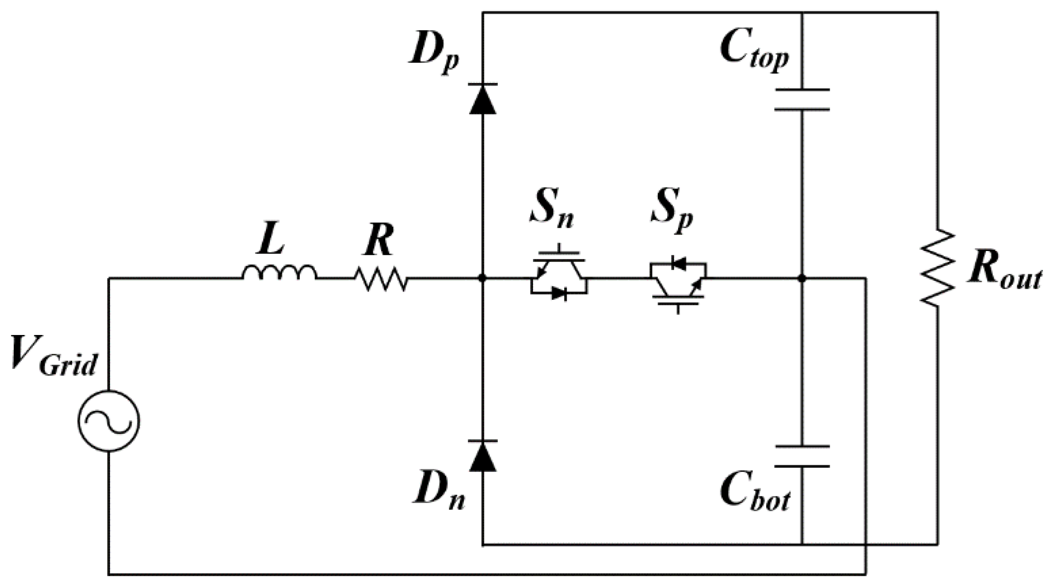
The Vienna rectifier discussed in this paper is similar in structure to a T-type inverter. However, in this device the outer switches are substituted for diodes, D_p and D_n, as shown in Figure 1, which restrict the flow of energy from DC to AC. Furthermore, we consider a single-phase topology, for application to the on board charger (OBC) of an EV, because of the simplified structure of this configuration, and its use of fewer switching devices [12,13,14,15].

To control a Vienna rectifier in normal operation, the “important rule”, defined as the sign of the voltage being equal to the sign of the current, should be satisfied. Failure to meet this criterion contributes to the degradation of current quality and an increase in total harmonic distortion (THD) [16]. Conventional Vienna rectifiers apply proportional-integral (PI) controllers to the line current control loop. These devices are optimized for regulating DC, and not AC components [17], as their dynamic response is not fast enough to control alternating current. Hence, an appropriate output cannot be estimated if a PI controller is used in an AC current control loop [18], and THD of the line current consequently increases [19,20]. Therefore, as the line current frequency increases and the system power decreases, the line current distortion problem becomes dominant [21].

In addition to large errors and the slow dynamic response of the PI controller, another reason for current distortion is a difference between the sensed current and the average current caused by discontinuous current mode (DCM) operation around the input voltage’s zero crossing point [22]. The phase difference between the input voltage and the line current also increases around this neutral region. Thus, to reduce the response error and alleviate problems associated with the DCM, a controller that has a fast dynamic response and can control the power factor (PF) to unity is necessary [23,24,25,26,27,28].

The predictive control method was researched to make the controller with faster dynamics. The predictive control is designed with the system model. Generally, in this method, the current is predicted by the past state data. The optimal duty cycle is derived by using this predicted current. Hence, the controller is possible to get the faster dynamics than the PI control method. As mentioned before, in order to deduce the optimal duty cycle, the current prediction is one of the important procedure. The study of [29] was considered for the next current prediction. The inductance model and simple mathematical method is used for calculating the predicted current.

In this paper, we propose a model-based predictive control algorithm for a single-phase Vienna rectifier, to improve the quality of its line current. The proposed controller has fast dynamics and simple algorithm. The optimal duty cycle for regulating the reference current in the shortest timescale is deduced by the controller algorithm predicting the next current state, and subsequently minimizing the error between the reference current and the line current. In addition, to control the rectifier in continuous current mode (CCM) and DCM operation separately, a mode detection algorithm is adopted. Hence, different optimized duty cycles for controlling the line current in CCM and DCM are deduced. In spite of this, the algorithm is capable of controlling the average line current, even if these two modes of operation are mixed. In contrast to PI control, the proposed algorithm has a fast dynamic response, making it possible for the line current to follow the reference current with the smallest error. Hence, the PF can be controlled to unity and THD of the line current can be decreased. We verify the operation of the proposed control algorithm using PSIM simulation and practical experiments performed with a 1-kW-rated single-phase Vienna rectifier prototype. Moreover, we compare the line current of a rectifier controlled using a conventional PI algorithm and the proposed algorithm, to demonstrate its performance.

2. Vienna Rectifier Control

2.1. Operation of the Vienna Rectifier

A circuit diagram of the single-phase Vienna rectifier employed in this study is shown in Figure 1. To the grid side, input filter of this topology is composed of inductor, L. The resistor, R, means the resistive component in the inductor. As previously stated, the topology of this device is similar to that of a single-phase T-type inverter, with the outer switches of the inverter having been replaced by the diodes D_p and D_n in the rectifier. The rectifier topology includes two inner switches, a top switch, S_p, which only operates when the top capacitor, C_top, is charging, and a bottom switch, S_n, which only operates while the bottom capacitor, C_bot, is charging. The detail nomenclature of the components is shown in

Table A1. Nomenclatures.

Variables/Acronyms/Indexes/Constants	Full Nomenclatures
EV	Electric Vehicle
MPC	Model-based Predictive Control
PWM	Pulse-Width Modulation
OBC	On Board Charger
THD	Total Harmonic Distortion
PF	Power Factor
FS-MPC	Finite StateModel-base Predictive Control
DSP	Digital Signal Processor
ADC	Analog to Digital Conversion
PI	Proportional-Integral
DCM	Discontinuous Current Mode
CCM	Continuous Current Mode
L	Filter inductor
R	Filter Resistor
VGrid	Grid Voltage
Dp	Top Diode of Vienna rectifier
Dn	Bottom Diode of Vienna rectifier
Sp	Top Switch
Sn	Bottom Switch
Ctop	Top Capacitor
Cbot	Bottom Capacitor
Rout	Output Resistor
VDC	DC Voltage
i*	Voltage Controller Output
iL	Sensed Inductor Current
iL*	Inductor Current Reference
ωcc	Bandwidth of PI controller
Kp,current	Proportional Gain of PI controller
KI,current	Integral Gain of PI controller
ζ	Damping-Ratio
ipeak	Peak Value of Inductor Current
iavg	Average Value of Inductor Current
izero	Zero Value of Inductor Current
SL,on	Slope during Switch on time
Vtop	Top DC link Voltage
Vbot	Bottom DC link Voltage
SL,bot,off	Slope during Bottom Switch off
SL,top,off	Slope during Bottom Switch on
iL,k + 1,top	Next State inductor Current
iL,k	Current State Inductor Current
ierr,top	Error of Inductor Current in CCM
Ton,top,CCM	Top Switch on Time in CCM
Dutytop,CCM	Top Switch Duty in CCM
Ton,bot,CCM	Bottom Switch on Time in CCM
Dutybot,CCM	Bottom Switch Duty in CCM
Tzero	Zero drop Time of Inductor Current
iL,avg,k + 1	Average Current of Next Current
ierr,DCM	Error in DCM
Ton,top,DCM	Top Switch on Time in DCM
Dutytop,DCM	Top Switch Duty in DCM
Ton,bot,DCM	Bottom Switch on Time in DCM
Dutybot,DCM	Bottom Switch Duty in DCM
L0	Actual Inductance Value
Lcal	Nominal Inductance Value

in appendix A. Figure 2 shows the equivalent circuit and the current path of a single-phase Vienna rectifier when the top switch is in operation. Figure 3 shows the equivalent circuit and the current path of a single-phase Vienna rectifier when the bottom switch is in operation.

Figure 2 and Figure 3 are further subdivided into different modes. Mode 1 and Mode 2 are operational when the grid voltage is positive, and Mode 3 and Mode 4 operate when the grid voltage is negative. When Mode 1 is in operation, both switches, S_p and S_n, are turned off. The line current flows through the top diode, D_p, and charges C_top. In Mode 2, S_p is turned on and the line current flows through this switch and the anti-parallel diode of S_n. The closed current path consists of the switching device and the neutral point of the DC link to the grid. The current path in Mode 3 is as with Mode 2. However, the direction of current flow is reversed in this mode. In Mode 4, S_n is turned off and current flow from the DC link to the grid side is in the same direction as in Mode 3. In this mode, the current path includes the bottom diode.

2.2. Conventional PI Control of a Vienna Rectifier

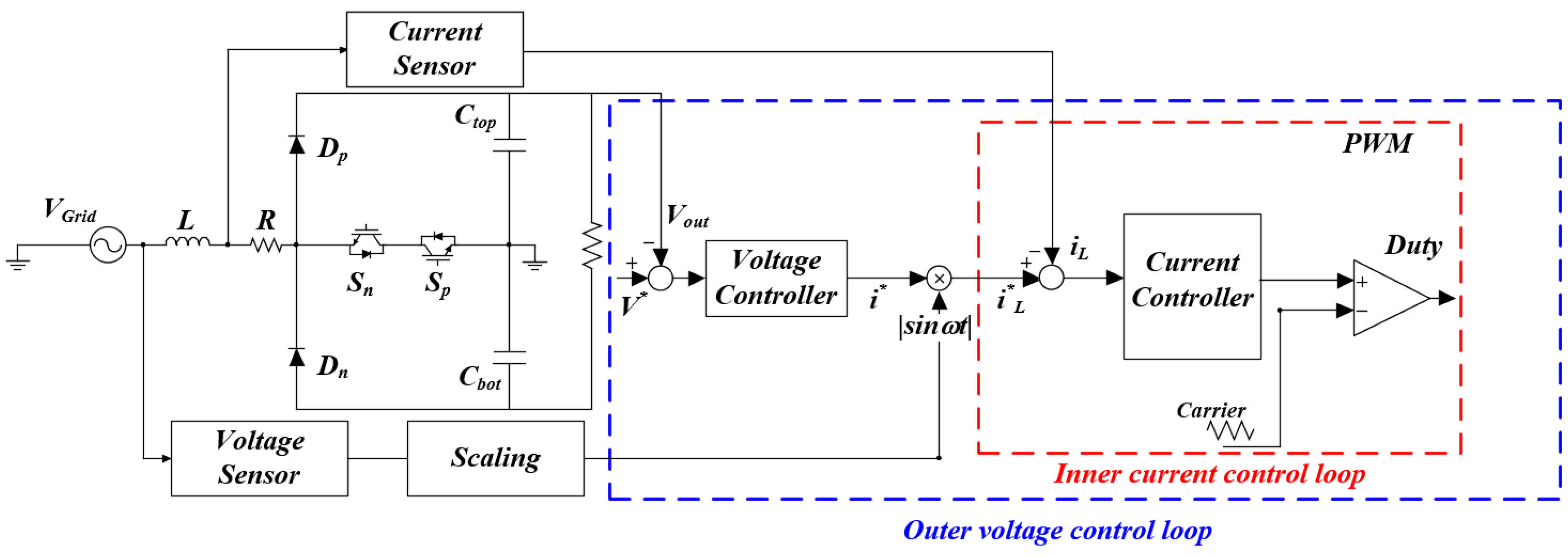
A block diagram of a complete Vienna rectifier system, including control circuitry, is shown in Figure 4. The voltage controller comprising the outer control loop consists of a PI controller, the input to which is the error between the sensed DC link voltage and the reference DC link voltage. The voltage controller of the conventional and proposed method applied system is same, both are PI controller. The output of the voltage controller is the reference current. In this image, sinωt is the waveform of the grid voltage, which is obtained by dividing the sensed grid voltage by its magnitude. The final line current reference, i_L^*, is obtained by multiplying i^* with sinωt. The input to the inner current control loop is the error between the sensed line current, i_L, and i_L^*. A PI controller is adopted for the current controller, the output of which is the PWM duty cycle. The bandwidth, ω_cc, of the current control loop should be wider than that of the voltage control loop. In addition, to prevent noise and disturbance, this ω_cc should be 1/20 or 1/10 of the switching frequency. Hence, the ω_cc of the system is limited by the switching frequency.

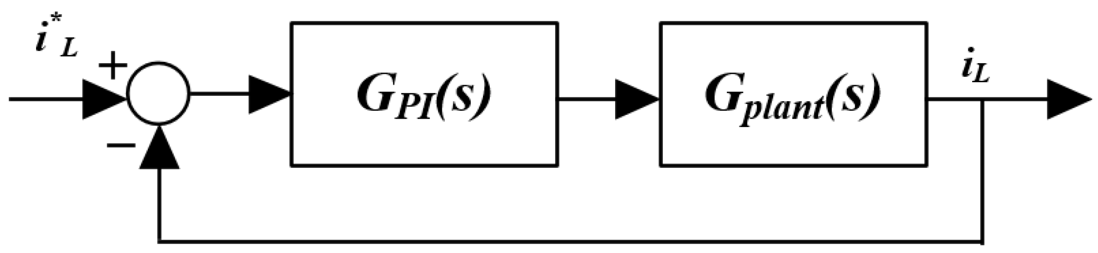
Figure 5 shows the closed current loop of the PI controller applied system. The G_PI(s) means the model of PI controller and G_plant(s) means the large signal mode of plant. G_PI(s) and G_plant(s) can be expressed as:

$$G_{PI}(s)=K_{p,current}(s)+\frac{K_{I,current}}{s},\hspace{0.17em}\hspace{0.17em}\hspace{0.17em}\hspace{0.17em}\hspace{0.17em}\hspace{0.17em}\hspace{0.17em}\hspace{0.17em}\hspace{0.17em}\hspace{0.17em}\hspace{0.17em}\hspace{0.17em}\hspace{0.17em}\hspace{0.17em}\hspace{0.17em}\hspace{0.17em}\hspace{0.17em}{G}_{plant}(s)=\frac{1}{sL},$$

(1)

where K_p,current is proportional gain (or P gain) of the current controller, K_I,current is integral gain (or I gain) of the current controller, L is the inductance of system. From (1) the closed current loop transfer function based on PI controller equation can be expressed as:

$$T(s)=\frac{G_{PI}{G}_{plant}}{1+G_{PI}{G}_{plant}},$$

(2)

Hence, the closed current loop transfer function based on PI controller, T(s), can be derived as:

$$T(s)=\frac{\frac{K_{I,current}}{L{s}^2}+\frac{K_{p,current}}{Ls}}{\frac{K_{I,current}}{L{s}^2}+\frac{K_{p,current}}{Ls}+1}.$$

(3)

By the characteristic equation of this transfer function, the P and I gain are simply derived as:

$$K_{p,current}=2\zeta {\omega }_{cc}L,\hspace{0.17em}\hspace{0.17em}\hspace{0.17em}\hspace{0.17em}\hspace{0.17em}\hspace{0.17em}\hspace{0.17em}\hspace{0.17em}\hspace{0.17em}\hspace{0.17em}\hspace{0.17em}\hspace{0.17em}\hspace{0.17em}\hspace{0.17em}\hspace{0.17em}\hspace{0.17em}\hspace{0.17em}{K}_{I,current}={\omega }_{cc}^{2}L.$$

(4)

where ζ is the damping-ratio. This value usually set as 0.707 for the critical damping characteristic. In (4) the gain of the PI controller contains the ω_cc. Thus, the gain of the controller is also limited by the switching frequency. As the gain of the PI controller employed in the current controller is limited, the regulation of the current is diminished when the input voltage crosses zero. As a result of the minimal control at this point, the current becomes distorted. One reason for this distortion is the slow dynamic response of the PI controller. The bandwidth of the controller is limited by the switching frequency, which also affects the dynamic response. The change in the AC reference around the zero-crossing section occurs too quickly for the controller to respond. The second reason for distortion is the variable mode of operation of the rectifier. In the CCM region, the average inductor current is equal to the sensed current. This means that the average current follows the reference current. In the DCM region, the average current does not match the sensed current and it thus cannot follow the reference current. Hence, a controller with a fast dynamic response and a mode detection algorithm is required to solve these problems.

2.3. Model-Based Predictive Control of a Single-Phase Vienna Rectifier

The model-based predictive control algorithm predicts the next current state and calculates the optimal duty cycle using data from previous states. Unlike the conventional PI control algorithm, this technique has a fast dynamic response, suitable for control of AC components. Therefore, it is possible to improve the line current distortion of the single-phase Vienna rectifier using the proposed algorithm. However, in the real situation when using a digital signal process (DSP), there is one cycle delay for an analog to digital conversion (ADC). Hence, in order to solve this problem, current prediction of two cycle after state is applied. Moreover, the precision of the model affects the performance of the controller. Thus, the compensation method for precise inductance model should be considered for the modelling of the controller.

2.3.1. Estimating the Gradient of the Inductor Current

The optimal duty cycle of a Vienna rectifier is derived using the predicted current and the gradient of the current flowing through the inductor. However, mode detection is required, as the shape of the line current is different in DCM and CCM operation. Hence, a mode detection method is also considered in addition to the current control method proposed in this paper.

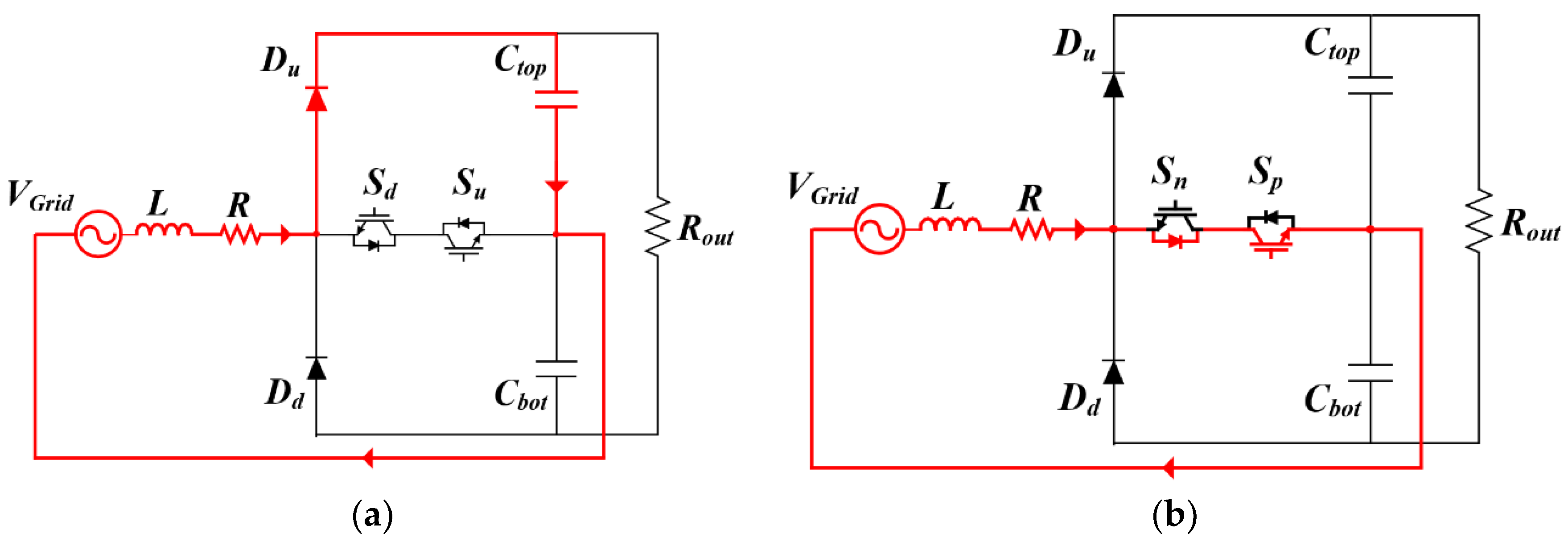
The current paths, when the top switch is off or on, are shown in Figure 6a,b, respectively. When the input voltage, V_Grid, is positive, the current flows through the switches if S_p is on, and through D_p if S_p is off. The voltage equation when the switch is on can be expressed as:

$$\left|V_{Grid}\right|-V_L=\left|V_{Grid}\right|-\left(L\frac{d{i}_L}{dt}+i_{L}R\right)=0,$$

(5)

where V_L is the voltage across the inductor and i_L is the inductor current that passes the resistor. The voltage applied to the inductor can be divided into two parts, one is voltage across the inductance component and another is voltage across the resistance of inductor. Equation (5) can be rearranged to obtain an expression for the slope, di_L/dt. Based on this rearranged equation, the slope of the current through the inductor when the switch is on, S_L,on, can be expressed as:

$$S_{L,on}=\frac{d{i}_L}{dt}=\frac{\left|V_{Grid}\right|-i_{L}R}{L}.$$

(6)

As V_Grid is positive in this sector, S_L,on is also positive. The voltage equation when the switch is off can be expressed as:

$$\left|V_{Grid}\right|=V_{top}+V_L=V_{top}+L\frac{d{i}_L}{dt}+i_{L}R,$$

(7)

where V_top is the voltage of the top DC link. As performed previously, (5) can be rearranged for the slope of the current as:

$$S_{L,top,off}=\frac{d{i}_L}{dt}=\frac{\left|V_{Grid}\right|-i_{L}R-V_{top}}{L},$$

(8)

where S_L,top,off is the slope of the inductor current when the top switch is off. As the DC link voltage is larger than |V_Grid| in the steady state, the value of the slope is negative. In this equation the DC link voltage is the difference between V_top and V_bot. Hence, the expression calculated for S_L,top,off is only suitable for when the top switch is in operation, and a different equation is required for the slope of the inductor current when the bottom switch is off. This can be obtained by substituting V_bot for V_top.

The slope of the inductor current when the bottom switch is in operation can be expressed similarly to (5)–(8). The equation for the current slope when the bottom switch is on is the same as (5), as the input voltage is an absolute value. However, when the bottom switch is off, V_bot is applied. Hence, the DC link voltage of the bottom capacitor, V_bot, is used instead of V_top, in the slope equation. The slope of the inductor current when the bottom switch is off, S_L,bot,off, can be expressed as:

$$S_{L,bot,off}=\frac{d{i}_L}{dt}=\frac{\left|V_{Grid}\right|-i_{L}R-V_{bot}}{L}.$$

(9)

The optimal duty cycle can thus be calculated using the slope equations given in (6), (8) and (9). However, considering the “skin effect” in the inductor, the R in slope equation has small value which is enough to ignore.

2.3.2. Deriving the Optimal Duty Cycle for CCM Operation

The inductor current during CCM, and the gate signal in the steady state region, are shown in Figure 7. In the steady state CCM region, the inductor current sensed by the digital processor is equal to the average inductor current. As such, the next inductor current state, i_{L,k + 1}, can be calculated using the current slopes previously derived as (6)–(8), and the present inductor current state, i_L,k, as:

$$i_{L,k+1,top}=i_{L,k}+S_{L,on}{T}_{on,top}+S_{L,top,off}\cdot (T_s-T_{on,top}),$$

(10)

where T_on,top,CCM is the period the top switch is on during CCM, T_off in Figure 7 is the period the switch is off, and T_s is the sampling period, which is the sum of T_on and T_off. The error, i_err, between i_{L,k + 1} and the line current reference, i_L^*, can be expressed as follows:

$$i_{err,top}=i_L^{*}-i_{L,k+1,top}=i_L^{*}-i_{L,k}-S_{L,on}{T}_{on,top}-S_{L,top,off}\cdot (T_s-T_{on,top})=0.$$

(11)

By rearranging (11), the on time interval for the duty cycle of the top switch can be derived as follows:

$$T_{on,top,CCM}=\frac{i_L^{*}-i_{L,k}-S_{L,top,off}\cdot T_s}{S_{L,on}-S_{L,top,off}}.$$

(12)

The optimal duty cycle for the top switch during CCM, Duty_top,CCM, can be expressed as follows:

$$Dut{y}_{top,CCM}=\frac{T_{on,top}{}_{,CCM}}{T_s}.$$

(13)

The optimal duty cycle of the bottom switch during CCM, Duty_bot,CCM, can be derived in a similar manner. Using the inductor current slope of the bottom switch, Duty_bot,CCM can be written as:

$$T_{on,bot,CCM}=\frac{i_L^{*}-i_{L,k}-S_{L,bot,off}\cdot T_s}{S_{L,on}-S_{L,bot,off}},$$

(14)

$$Dut{y}_{bot,CCM}=\frac{T_{on,bot}{}_{,CCM}}{T_s},$$

(15)

where T_on,bot,CCM is the period of time that the bottom switch is on during CCM.

2.3.3. Deriving the Optimal Duty Cycle for DCM Operation

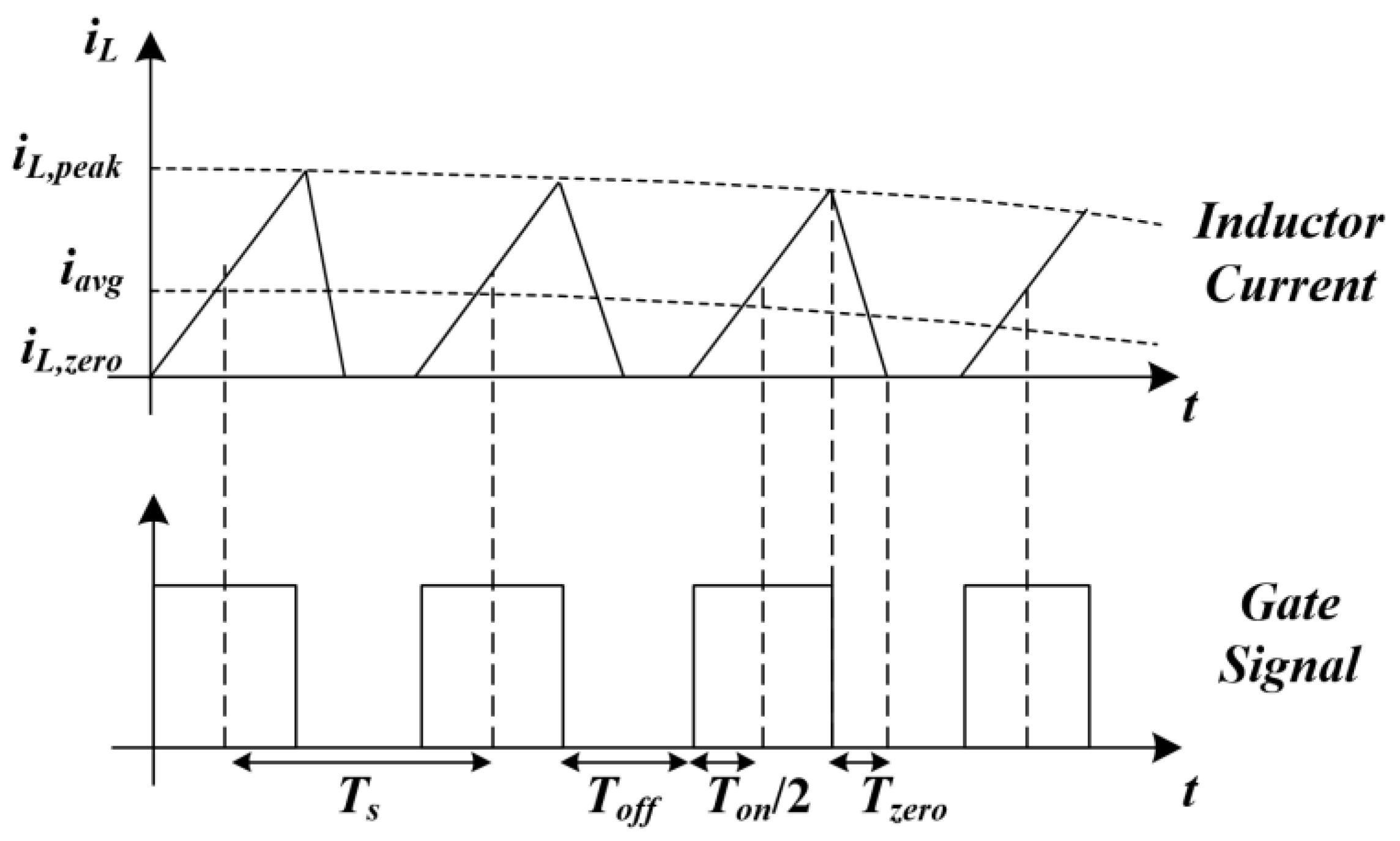
The steady state inductor current and gate signal during DCM are shown in Figure 8. In this mode of operation, the average inductor current is different to the sensed inductor current. Furthermore, the sum of the rise time and fall time does not correspond to the value of T_s. Hence, the inductor current is improperly regulated with respect to the applied reference current when the current control algorithm developed for CCM is applied in DCM. An appropriate optimal duty cycle prediction method is thus required for DCM.

The optimal duty cycle for DCM operation can be deduced by applying a similar method to that used for CCM. The peak inductor current equation can be expressed as follows:

$$i_{L,peak}=S_{L,on}\cdot T_{on}=-S_{L,top,off}\cdot T_{zero},$$

(16)

where T_zero is the time required for i_L,peak to be reduced to i_L,zero. From (16), T_zero can be expressed as:

$$T_{zero}=-\frac{S_{L,on}{T}_{on}}{S_{L,top,off}}.$$

(17)

In DCM, the next average inductor current state can be calculated using integration as follows:

$$i_{L,avg,k+1}=\frac{1}{T_s}{\displaystyle {\int }_{T_s}^{}{i}_L\hspace{0.17em}dt=\frac{i_{L,peak}\cdot \left(T_{on}+T_{zero}\right)}{2\cdot T_s}}.$$

(18)

The error can be calculated in a similar manner to (10) as:

$$i_{err,DCM}=i_L^{*}-i_{L,avg,k+1}.$$

(19)

By rearranging (19), the on time interval can be expressed as follows:

$$T_{on,top,DCM}=\sqrt{2\cdot i_L^{*}\cdot T_s/S_{L,on}\cdot \left(1-\frac{S_{L,on}}{S_{L,top,off}}\right)},$$

(20)

where T_on,top,DCM is the duration the top switch is on during DCM. The optimal duty cycle of the top switch during DCM, Duty_top,DCM, can be expressed as follows:

$$Dut{y}_{top,DCM}=\frac{T_{on,top}{}_{,DCM}}{T_s}.$$

(21)

The optimal duty cycle of the bottom switch during DCM, Duty_bot,DCM, can be derived in a similar manner. Using the current slope expression for the bottom switch, Duty_bot,DCM can be written as:

$$T_{on,bot,DCM}=\sqrt{2\cdot i_L^{*}\cdot T_s/S_{L,on}\cdot \left(1-\frac{S_{L,on}}{S_{L,bot,off}}\right)},$$

(22)

$$Dut{y}_{bot,DCM}=\frac{T_{on,bot,DCM}}{T_s},$$

(23)

where T_on,bot,DCM is the period the bottom switch is on during DCM. Using the optimal duty cycles calculated with (13), (15), (21) and (23), it is possible to control the system with a faster dynamic response than a PI controller.

2.3.4. Mode Detection for the Vienna Rectifier

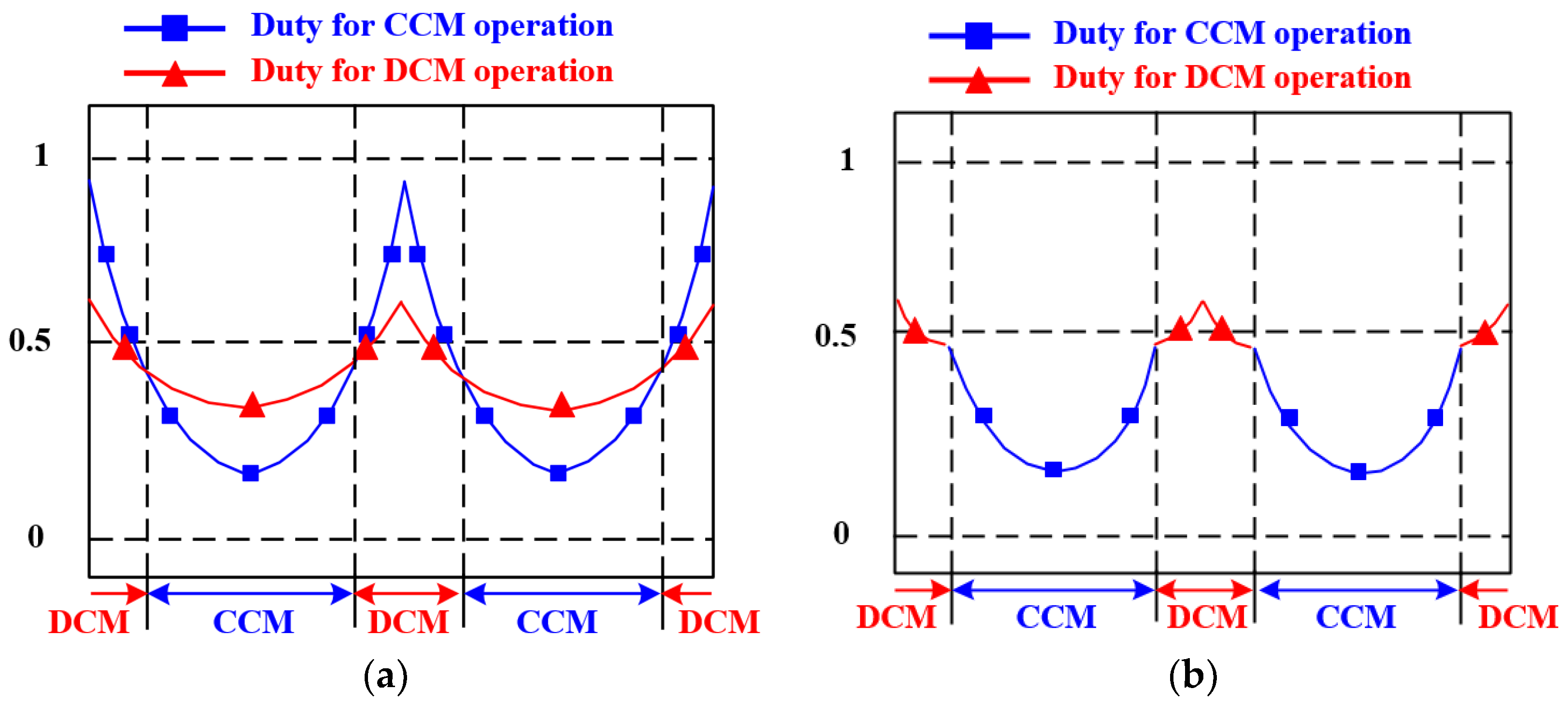
The average current in both the heavy load and light load conditions are controllable using the duty cycles optimized for CCM and DCM operation, respectively. However, in the medium load condition where both conduction modes coexist, the appropriate control method should be determined for the relevant mode of operation. During DCM operation, the duty cycle calculated using the CCM equation is always larger than the duty cycle calculated using the DCM equation. In contrast, during CCM operation, the duty cycle calculated using the DCM equation is always larger than the duty cycle calculated using the CCM equation. Therefore, by verifying the smaller duty cycle in the present state of operation, it is possible to select the appropriate duty cycle for each mode. Figure 9 shows the operation of the mode detection method. The regions where the duty cycles for CCM and DCM intersect are shown in Figure 9a. At these intersection points, the conduction mode of the rectifier changes. By applying the criterion defined in the mode detection method, it is possible to select the optimal duty cycle for the relevant conduction mode, as illustrated in Figure 9b.

2.3.5. System Stability of Proposed Predictive Control Method

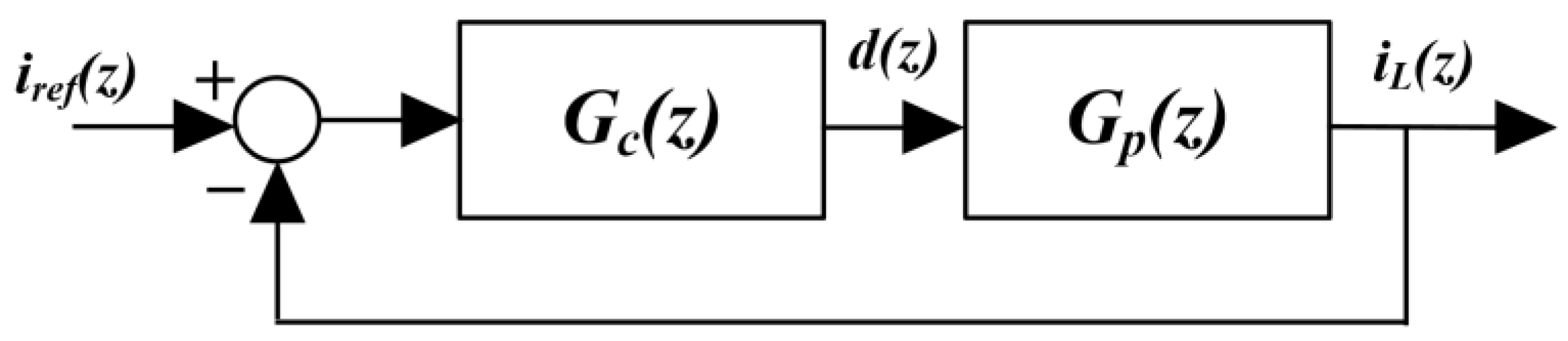
The proposed method calculates the optimal duty cycle by the inductance value. Hence, the performance of controller depends on the preciseness of the inductance model. The inductance value can be changing by the experimental ambient. Therefore, it is important to consider this inductance value variation. In order to confirm the stability of the proposed method, z-plane discriminant analysis is used. The block diagram of simple system model is shown in Figure 10.

The rectifier system is simply derived by the small signal model of the voltage equation of inductor as:

$$G_p(s)=\frac{i_L\left(s\right)}{d\left(s\right)}=\frac{V_{DC}}{s{L}_0},$$

(24)

where, L₀ is the actual inductance value with considering inductance value changing. Then changing this equation to the z-domain the equation is rearranged as:

$$G_p(z)=\frac{i_L\left(z\right)}{d\left(z\right)}=\frac{V_{DC}{T}_s}{L_0}\left(\frac{z^{-1}}{1-z^{-1}}\right),$$

(25)

As shown in this figure, z-domain equation of the controller is simply model with the (5), (7) and (11) as:

$$G_c(z)=\frac{d\left(z\right)}{i_e\left(z\right)}=\frac{L_{cal}}{V_{DC}{T}_s},$$

(26)

where L_cal is the nominal inductance value without considering of inductance value changing. The transfer function of the system is derived by (25) and (26) as:

$$H(z)=\frac{G_c(z)G_p(z)}{1+G_c(z)G_p(z)}=\frac{z^{-1}}{1+(K-1)z^{-1}},$$

(27)

where K = (L_cal/L₀). From (27), the system pole is calculated as:

$$z=1-K.$$

(28)

The system pole is in the unit circle on the z-plane, it is possible to confirm the system is stable. Figure 11 shows the simulation results of system poles of the proposed controller on z-plane with using MATLAB. When the L₀ is changed to the 50% error of its value, the system pole is on the unit circle and the L₀ is closer to the L_cal the system pole became closer to the origin. Thus, considering this simulation results, the inductance error should be less than 50% of L_cal in order to make the system stable. As the L₀ increased, the system pole is moving from origin to the positive side of unit circle.

2.3.6. Consideration of Inductance Variation

As mentioned in the previous section, the inductance variation affects to the controllability of the proposed method. The actual inductance value became different to the nominal inductance by the out ambient. This makes the changing of the calculation result of the inductor current slope. Hence, the inductance compensation method is necessary for the proposed control. The researches of [30,31,32] the compensation method for the inductance is introduced. This paper adopts the simple mathematical method of [32] for the inductance value compensation.

The next inductor current is decided by the next state inductance value and the current state of duty and the inductance value. Hence, by using this relation, the actual inductance is possible to be estimated on line. The equation for the online inductance estimation can be expressed as:

$$L_{k+1}=\left[\frac{i_{L,k}\cdot Dut{y}_k}{i_{L,k+1}\cdot Dut{y}_{k+1}}\right]L_k,$$

(29)

where L_k is the current state of online-estimated inductance, L_{k + 1} is the current next of online-estimated inductance i_L,k is the current state of the inductor current, i_{L,k + 1} is the next state of inductor current, Duty_k is the optimal duty cycle in current state and Duty_k+1.

3. Simulations

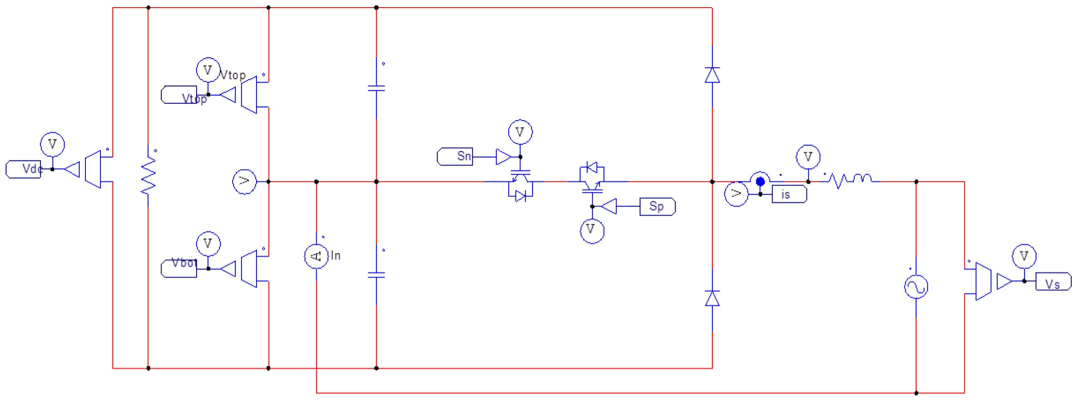
To verify the operation of the proposed algorithm, we performed a simulation using PSIM software. Figure 12 shows a schematic of the 1-kW-rated single-phase Vienna rectifier used in simulation. Moreover, both the top and bottom DC voltage are sensed, for calculating the optimal duty cycle of the model-based predictive controller (MPC). The input voltage of the system is 110 V_rms, varied at 60 Hz. The DC link voltage is controlled to 350–400 V. The controller should conduct one control operation per one control period because the proposed method should predict the next state current based on system model. Hence the sampling time is selected as 100 µs. Detailed simulation parameters are given in

Table 1. Simulation parameters.

Parameter	Value
Rated power	1 kW
Grid side voltage	110 Vrms
DC-link voltage	350–400 V
Inductor	1 mH
Top/Bottom Capacitor	450 µF
Grid frequency	60 Hz
Switching frequency	10 kHz
Sampling time	100 µs

.

The control algorithms for DCM and CCM operation were verified using a light load condition, defined as 20% of the maximum load, and a heavy load condition, defined as 100% of the maximum load, respectively. To compare the differences between the operation of a PI controller and the MPC, simulations were conducted with a 40% load and a full load. The THD of the resulting current waveforms were used as the standard for comparison.

Figure 13 shows the current waveform derived using the PI controller with a 20% load. The rectifier is in DCM in this load condition, making it difficult for the PI controller to regulate the line current to the reference current. Figure 14 shows the current waveform derived using the PI controller in the 100% load condition. Even though the rectifier is in CCM, the slow dynamic response of the PI controller contributes to the distortion of the line current. Therefore, the line current does not fully mirror the reference current.

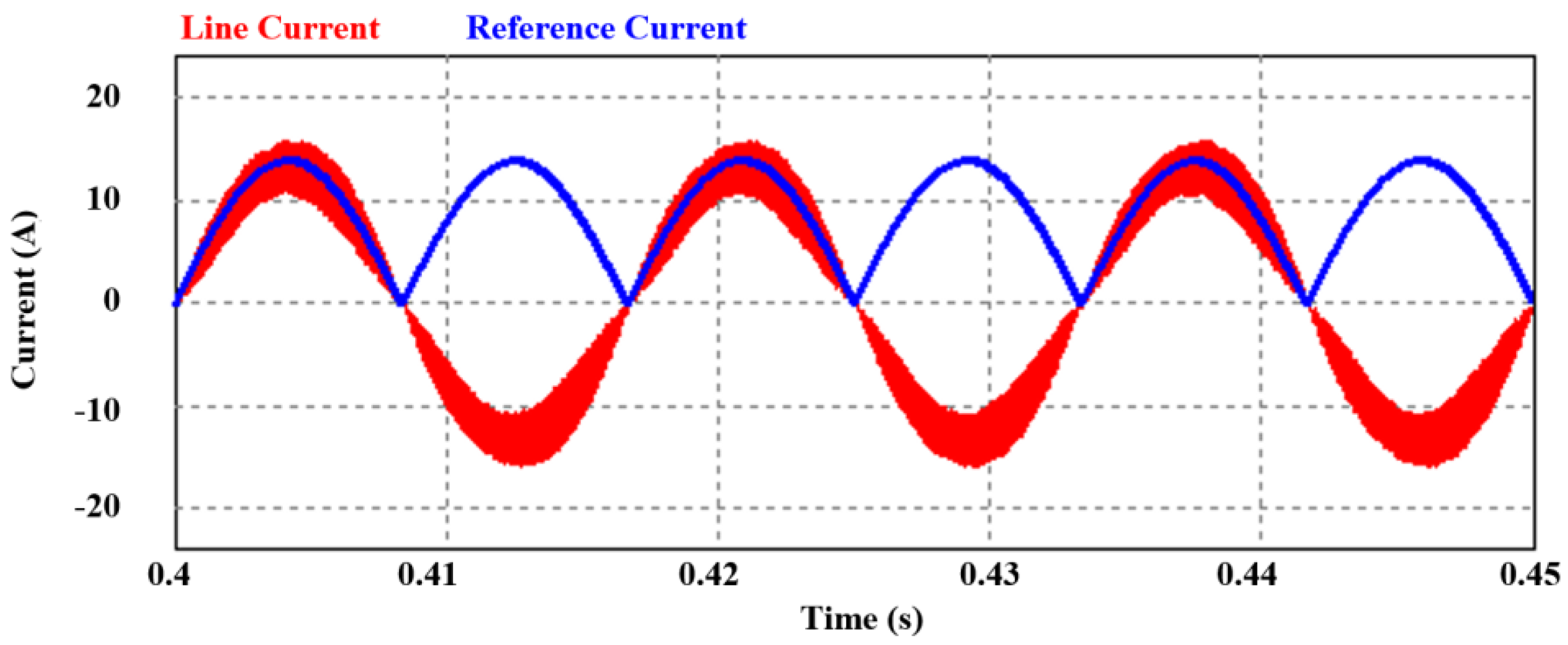
Figure 15 shows the current waveform derived using the MPC with a 20% load. Although the rectifier is in DCM, the proposed MPC algorithm is able to regulate the line current to the reference current. As mode detection was applied, a suitable duty cycle for DCM was generated. Figure 16 shows the current waveform derived using the MPC in the 100% load condition. The MPC-regulated system is able to mirror the reference current in the CCM region without problems, due to the fast dynamic response of the control algorithm. A comparison of the waveforms generated using the two systems shows that in DCM and CCM operation, there is more distortion in the current waveforms created with the PI-controlled system than those observed with the MPC-regulated system. The mode detection applied with the MPC makes it able to control the line current optimally in each conduction mode. In addition, the dynamic response of the controller is fast enough to control AC waveforms.

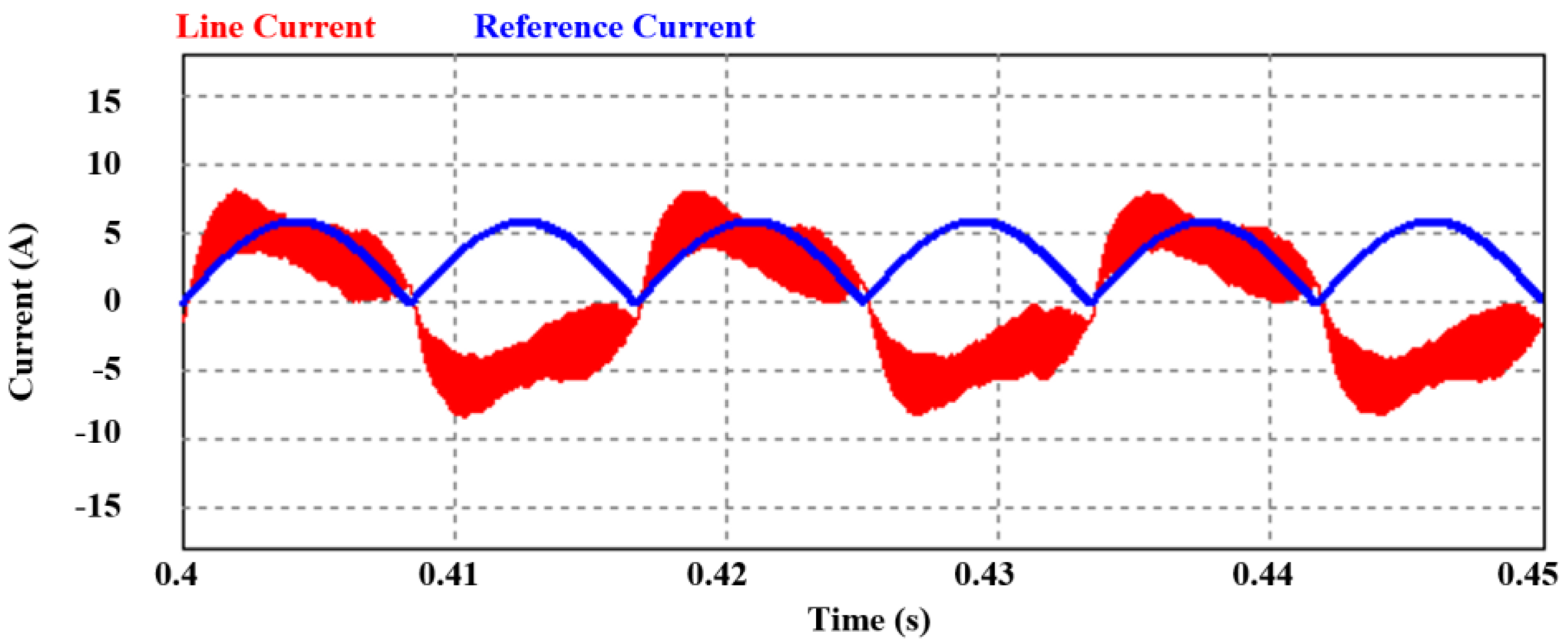
Figure 17 shows the current waveform derived using PI control with a 40% load, in the time domain. In the low load region, current distortion is made worse by prolonged operation in DCM. As shown in Figure 17, it is difficult for the line current to mirror the reference current. This current distortion becomes more apparent with a low power load. In particular, the distortion is worsened near the zero-crossing point of the current. Figure 18 shows the corresponding current waveform in the frequency domain. With this figure, the harmonic components of the current can be observed.

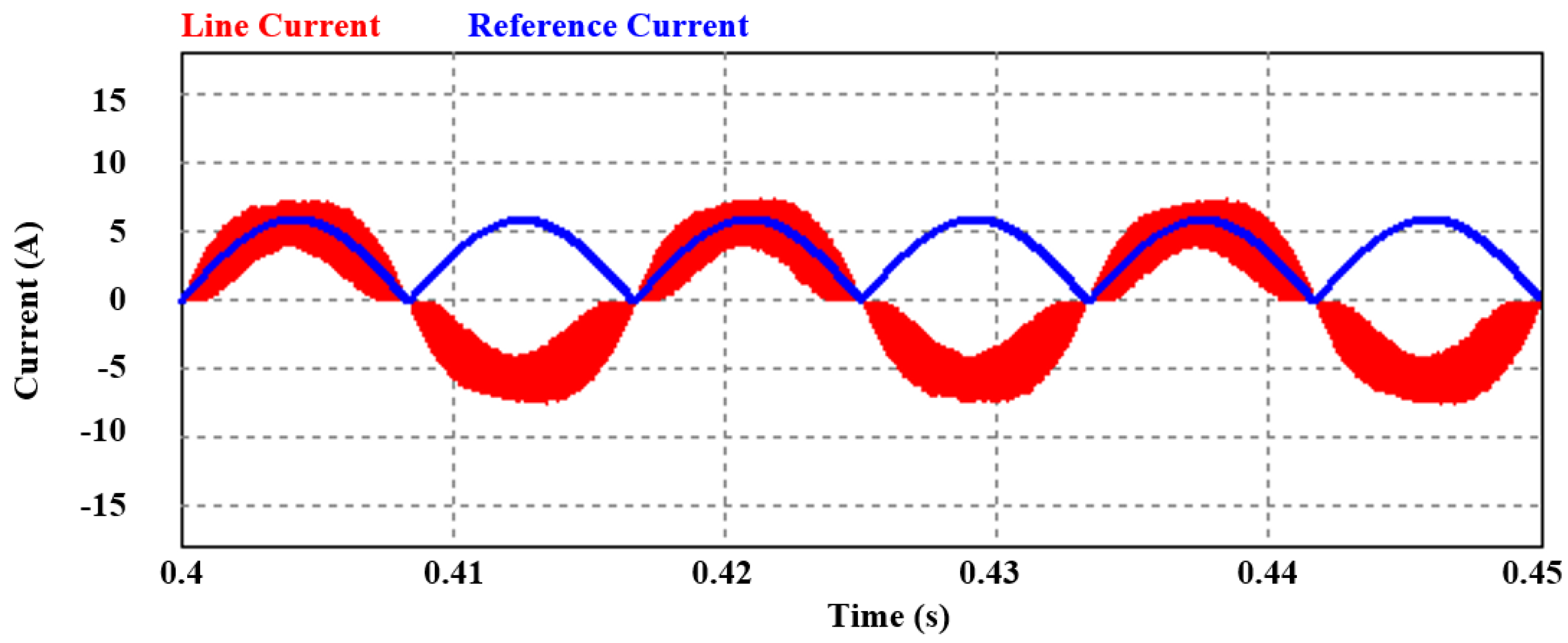
Figure 19 shows the current waveform derived using the MPC with a 40% load, in the time domain. With this algorithm, the line current is closer to the reference current. The difference in current quality between the conventional and proposed algorithms can be observed at the zero-crossing points of the line current. At these points, the rate of change of current is steepest. Hence, in order to regulate this quick change, a controller with a fast dynamic response is required. The MPC deduces the optimal duty cycle for both the CCM and DCM. Hence, unlike the PI controller, it is capable of this faster dynamic response. Figure 20 shows the current waveform derived using the MPC, in the frequency domain. In contrast to the waveform observed with conventional PI control, the magnitude of the harmonics in the MPC-regulated system is too small to observe, indicating that the MPC improves line current quality.

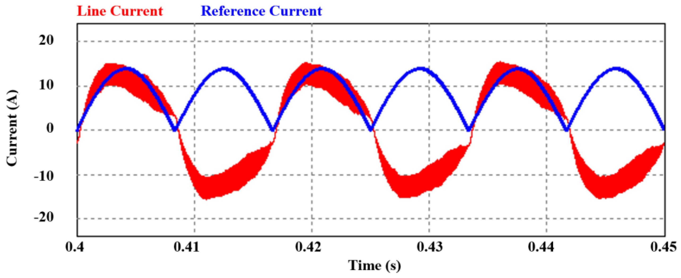
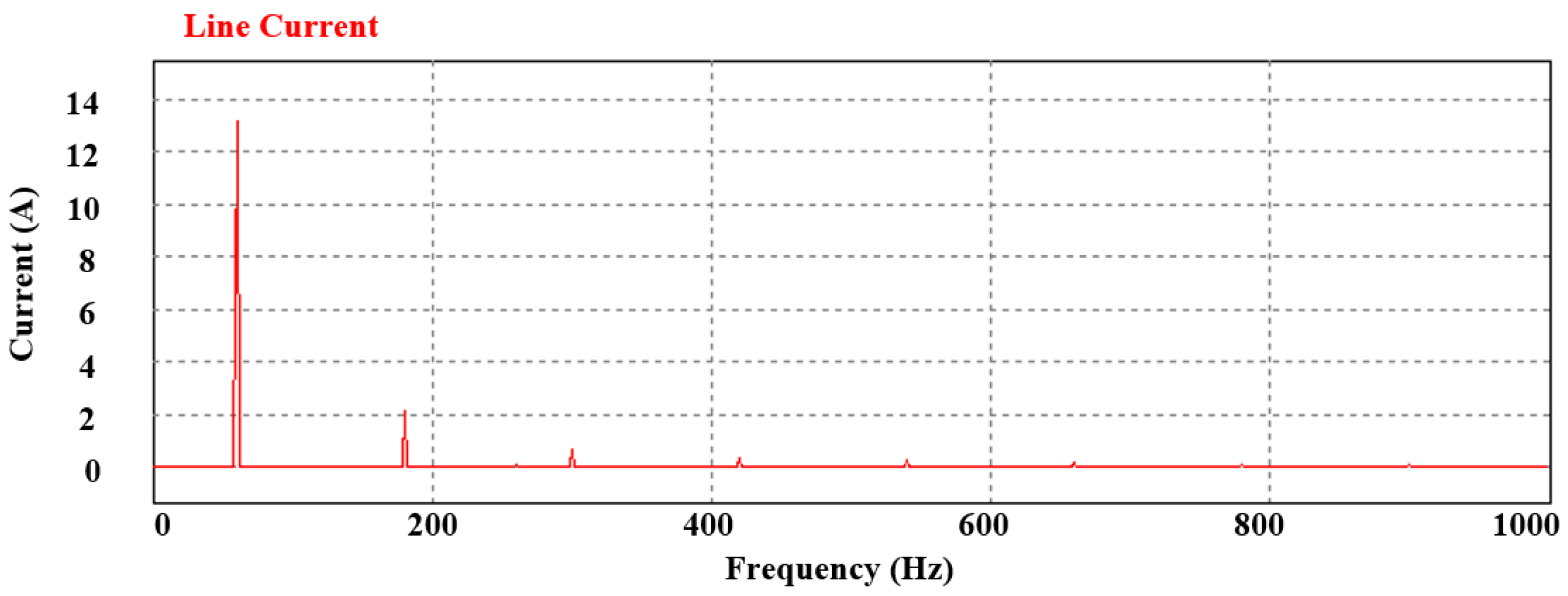
Figure 21 shows the current waveform derived using PI control, with a full load, in the time domain. In high load conditions, the rectifier operates predominantly in CCM. Although, there is little DCM operation, it is possible to observe current distortion with the conventional PI control method, which is confirmed by analysis of the current in the frequency domain, as shown in Figure 22. From this image, it can be observed that the magnitude of the harmonic components generated is approximately 10% of the magnitude of the fundamental current component.

Figure 23 shows the current waveform derived using the MPC, with a full load, in the time domain. Based on this image, it can be observed that line current distortion is greatly decreased with this system, in comparison to the distortion generated with the PI-controlled system. Furthermore, the distortion near the zero-crossing point is also decreased. Figure 24 shows the corresponding waveform in the frequency domain, where only the fundamental current component can be observed. When all regions of the current waveform are considered in total, including the zero-crossing points where the line current abruptly changes, we observe that the fast dynamic response of the MPC is able to decrease line current distortion.

4. Experimental Section

Figure 25 shows the components used in the practical experiments. These include the single-phase Vienna rectifier prototype, depicted in Figure 25a, and the control circuitry, shown in Figure 25b, which was installed on the rectifier. The MPC algorithm was programmed on a TMS320F28335 digital signal processor (DSP). In addition, the THD and PF were measured using a WT-3000 power analyzer (Yokogawa, Tokyo, Japan). The experimental parameters are the same as the simulation parameters.

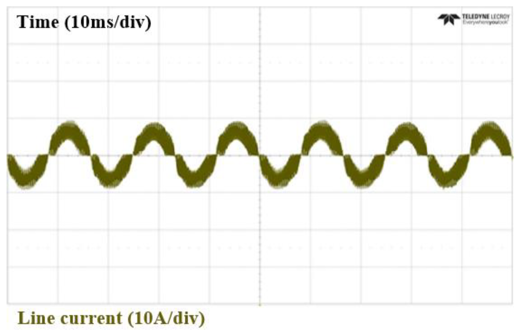
Figure 26 shows the line current waveform generated when conventional PI control was applied at 40% of the rated power. In this load condition, DCM operation is dominant. Hence, current distortion is appreciable due to prolonged operation in DCM. Moreover, the dynamic response of the PI controller is not fast enough to regulate the line current.

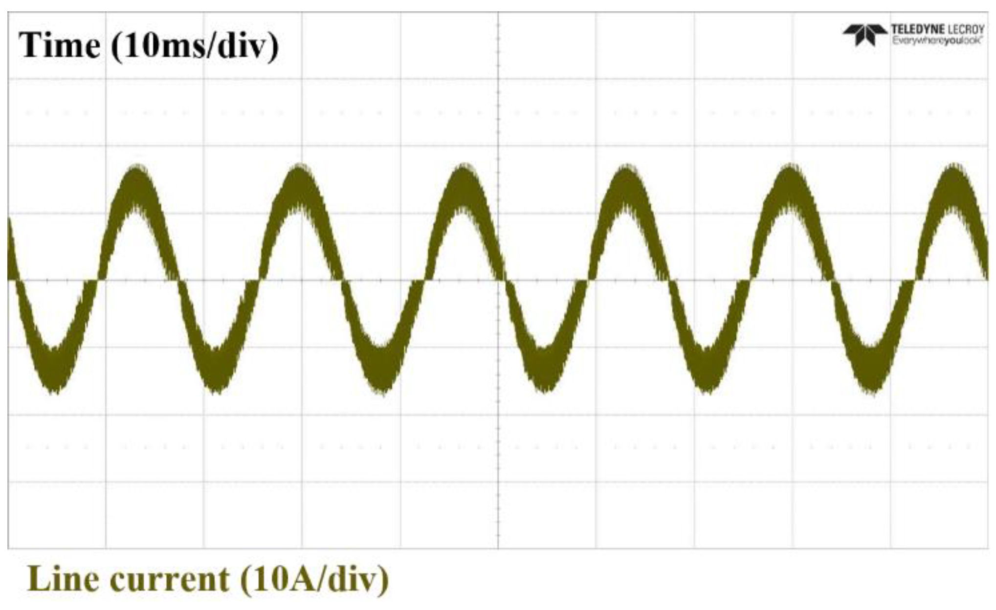
Figure 27 shows the waveform generated when the proposed MPC algorithm was applied at 40% of the rated power. The MPC deduces the optimal duty cycle for control based on the system model, improving line current quality as a result of its fast dynamic response. This means that, with this algorithm, it is possible to improve the THD and the PF of the line current.

Figure 28 shows the current waveform observed when conventional PI control was applied at rated power. Near the zero-crossing point, where the line current changes quickly, the slow dynamic response of the PI controller induces distortion. With this method, we also observe an increase in harmonic current components and a decrease in the PF, indicating a deterioration of the line current quality. Figure 29 shows the current waveform generated when the proposed MPC algorithm was applied at rated power. In contrast to the PI-controlled system, the distortion near the zero-crossing point is decreased. This image indicates that the line current mirrors the reference current.

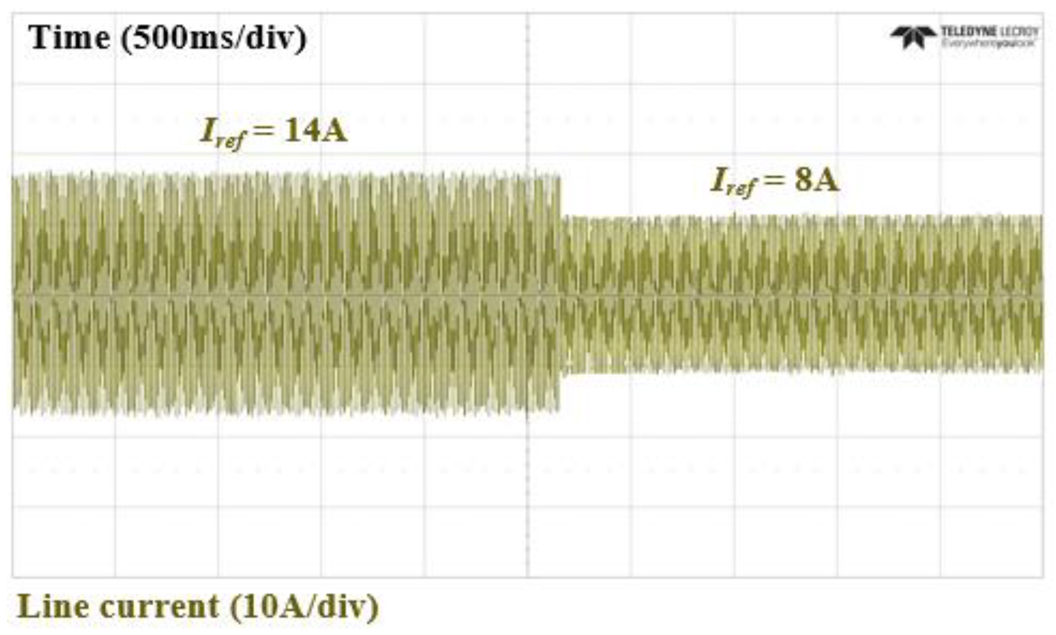
Figure 30 shows the transient of line current when the load is suddenly changed 60 to 100%. In this figure, it is possible to see that the transient waveform has low overshoot and fast convergence to the steady state region. Figure 31 shows the transient of line current when the load is suddenly changed 100 to 60%. This figure shows same manner as the previous waveform. This shows that the line current is possible to control the sudden load changing without any problems.

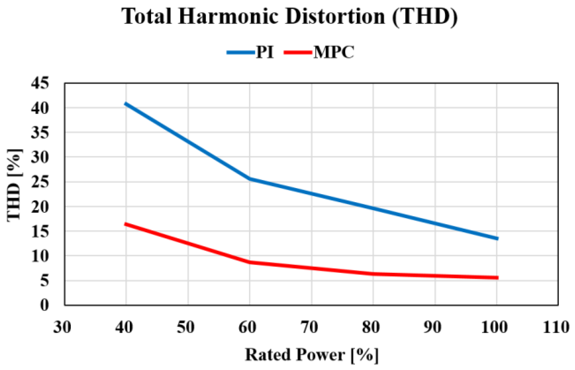
Figure 32 shows the THD in the different load conditions. In the PI-controlled system, THD is 40.68% at 40% of the rated power, and 13.49% at the rated power. In the MPC-regulated system, THD is 16.36% at 40% of the rated power, and 5.52% at the rated power. When the load is increased, the THD is improved, regardless of if the PI controller or the MPC is applied. With the proposed MPC algorithm, the value of the THD is approximately about 7–15% lower than the value obtained with conventional PI control, in all load conditions.

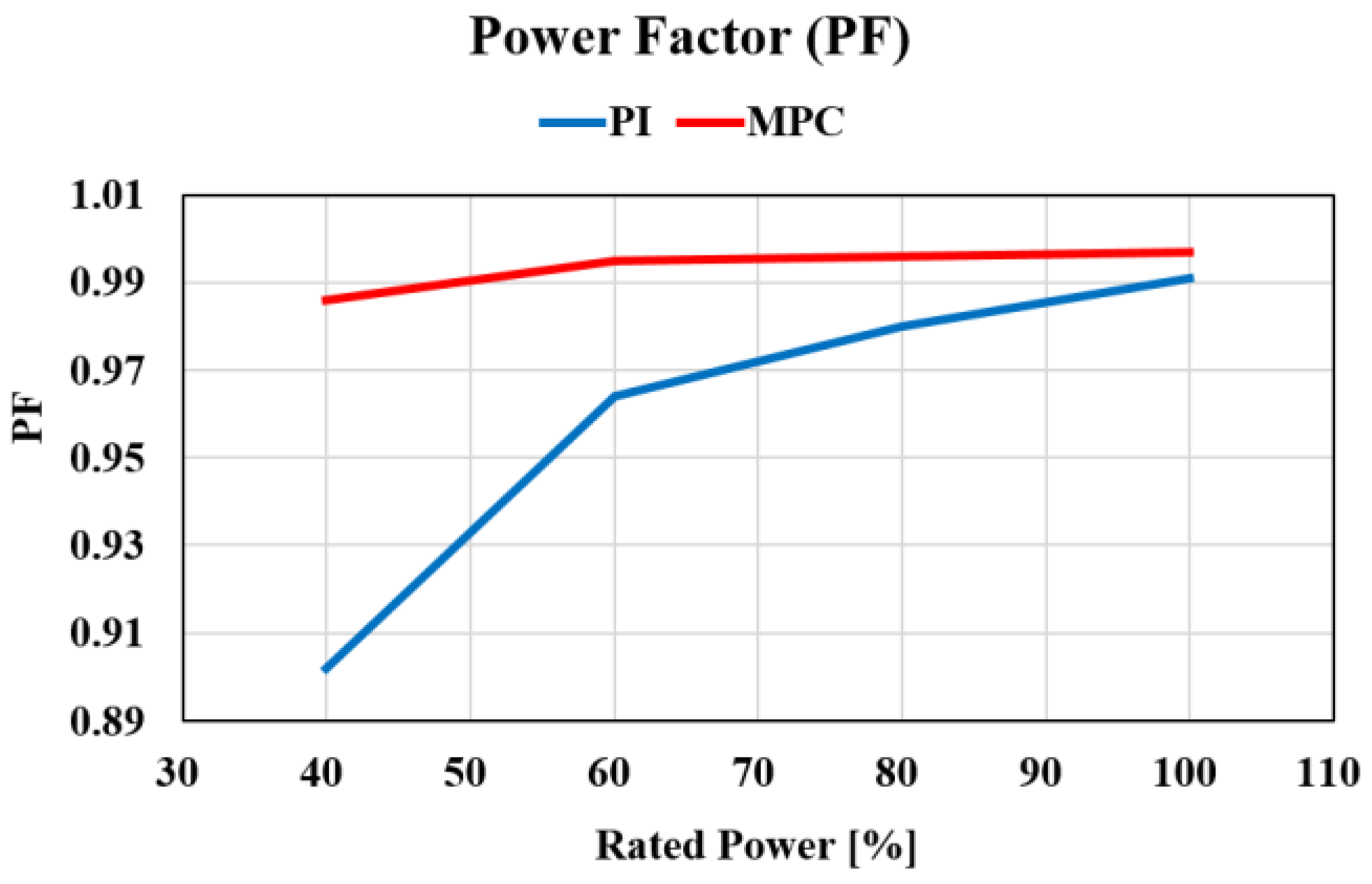
Figure 33 shows the value of the PF in the different load conditions. With the PI-controlled system, the value of the PF is 0.902 with the 40% load and 0.991 at rated power. In contrast, with the MPC-regulated system, the value of the PF is 0.986 at 40% of the rated power, and 0.997 at rated power. Hence, with both control systems, the PF is brought closer to unity by increasing the load. As the fundamental current component is increased in proportion to the harmonics, the PF is improved, and THD is alleviated. The performance of the proposed MPC algorithm can thus be verified using these two figures.

5. Conclusions

This paper proposes the improvement of the line current distortion for the single-phase Vienna rectifier using the model-based predictive control. Moreover, the conduction mode detection method is applied to the proposed MPC algorithm. The proposed algorithm conducts the prediction of the optimal duty cycle by using the previous and the current data of the inductor current. Therefore, this makes the proposed method possible to have the fast dynamic response, unlike the conventional PI control method. The PSIM simulation and the experimental result with the 1-kW single-phase Vienna rectifier are used for verifying the performance of the proposed algorithm. The current waveforms of the conventional method and the proposed method are compared. Moreover, THD and PF in the various load condition is measured in order to prove the validity of the proposed MPC algorithm.

References

- Bak, Y.S.; Lee, E.S.; Lee, K.-B. Indirect Matrix Converter for Hybrid Vehicle Application with Three-Phase and Single Outputs. Energies 2015, 8, 3849–3866. [Google Scholar] [CrossRef]
- Kim, J.-H.; Lee, I.-O.; Moon, G.-W. Integrated Dual Full-Bridge Converter With Current-Doubler Rectifier for EV Charger. IEEE Trans. Power Electron. 2016, 31, 942–951. [Google Scholar] [CrossRef]
- Lee, J.-H.; Lee, J.-S.; Lee, K.-B. A Fault Diagnosis Method in Cascaded H-bridge Multilevel Inverter Using Output Current Analysis. J. Electr. Eng. Technol. 2017, 12, 2278–2288. [Google Scholar]
- Park, J.Y.; Sin, J.O.; Bak, Y.S.; Lee, K.-B. Common-mode Voltage Reduction for Inverters Connected in Parallel Using and MPC Method with Subdivided Voltage Vectors. Journal of Electrical Engineering & Technology 2018, 13, 1212–1222. [Google Scholar]
- Jeong, M.-G.; Kim, S.-M.; Lee, K.-B. Discontinuous PWM Scheme for Switching Losses Reduction in Modular Multilevel Converters. J. Power Electron. 2017, 17, 1490–1499. [Google Scholar]
- Park, J.-H.; Yang, S.H.; Lee, K.-B. Synchronous Carrier-based Pulse Width Modulation Switching Method for a Vienna Rectifier. J. Power Electron. 2018, 18, 604–614. [Google Scholar]
- Jeong, M.-G.; Kim, S.-M.; Lee, K.-B. An Interleaving Scheme for DC-Link Current Ripple Reduction in Parallel-Connected Generator Systems. J. Power Electron. 2017, 17, 1004–1013. [Google Scholar]
- Yang, S.H.; Park, J.-H.; Lee, K.-B. Current Quality Improvement for a Vienna Rectifier with High-Switching Frequency. Trans. Korean Inst. Power Electron. 2017, 22, 181–184. [Google Scholar] [CrossRef]
- Wu, H.; Zhang, Y.; Jia, Y. Three-Port Bridgeless PFC Based Quasi Single-Stage Single-Phase AC-DC Converters for Wide Voltage Range Applications. IEEE Trans. Ind. Electron. 2018, 65, 5518–5528. [Google Scholar] [CrossRef]
- Adhikari, J.; Prasanna, I.V.; Panda, S.K. Reduction of Input Current Harmonic Distortions and Balancing of Output Voltages of the Vienna Rectifier under Supply Voltage Disturbances. IEEE Trans. Power Electron. 2017, 32, 5802–5812. [Google Scholar] [CrossRef]
- Kim, D.-H.; Kim, M.-J.; Lee, B.-K. An Integrated Battery Charger with High Power Density and Efficiency for Electric Vehicles. IEEE Trans. Power Electron. 2017, 32, 4553–4565. [Google Scholar] [CrossRef]
- Kwon, M.; Choi, S. An Electrolytic Capacitorless Bidirectional EV Charger for V2G and V2H Applications. IEEE Trans. Power Electron. 2017, 32, 6792–6799. [Google Scholar] [CrossRef]
- Thangavelu, T.; Shanmugam, P.; Raj, K. Modelling and control of VIENNA rectifier a single phase approach. IET Power Electron. 2015, 8, 2471–2482. [Google Scholar] [CrossRef]
- Lee, J.-S.; Lee, K.-B. Performance Analysis of Carrier-Based Discontinuous PWM Method for Vienna Rectifiers with Neutral-Point Voltage Balance. IEEE Trans. Power Electron. 2016, 31, 4075–4084. [Google Scholar] [CrossRef]
- Lee, J.-S.; Lee, K.-B. Predictive Control of Vienna Rectifiers for PMSG Systems. IEEE Trans. Ind. Electron. 2017, 64, 2580–2591. [Google Scholar] [CrossRef]
- Lee, J.-S.; Lee, K.-B. A Novel Crrier Based PWM for Vienna Rectifier with a Variable Power Factor. IEEE Trans. Ind. Electron. 2016, 63, 3–12. [Google Scholar] [CrossRef]
- Mallik, A.; Lu, J.; Khaligh, A. A Comparative Study between PI and Type-II Compensators for H-Bridge PFC Converter. IEEE Trans. Ind. Appl. 2018, 54, 1128–1135. [Google Scholar] [CrossRef]
- Pastor, M.-A.; Idiarte, V.-E.; Pastor, C.-A.; Salamero, M.-L. Interleaved Digital Power Factor Correction Based on the Sliding-Mode Approach. IEEE Trans. Power Electron. 2016, 31, 4641–6453. [Google Scholar] [CrossRef]
- Kanaan, H.Y.; Al-Haddad, K.; Hayek, A.; Mougharbel, I. Design, study, modelling and control of a new single-phase high power factor rectifier based on the single-ended primary inductance converter and the Sheppard-Taylor topology. IET Power Electron. 2007, 2, 163–177. [Google Scholar] [CrossRef]
- Malik, A.; Khaligh, A. An Integrated Control Strategy for a Fast Start-Up and Wide Range Input Frequency Operation of a Three-Phase Boost-Type PFC Converter for More Electric Aircraft. IEEE Trans. Veh. Technol. 2017, 66, 10841–10852. [Google Scholar] [CrossRef]
- Louganski, K.P.; Lai, J.S. Current phase lead compensation in single-phase PFC boost converters with a reduced switching frequency to line frequency ratio. IEEE Trans. Power Electron. 2007, 22, 113–119. [Google Scholar] [CrossRef]
- Kim, D.J.; Park, J.-H.; Lee, K.-B. Scheme for Improving Line Current Distortion of PFC Using a Predictive Control Algorithm. J. Power Electron. 2015, 15, 1168–1177. [Google Scholar] [CrossRef]
- Ren, H.-P.; Guo, X. Robust Adaptive Control of a CACZVS Three-Phase PFC Converter for Power Supply of Silicon Growth Furnace. IEEE Trans. Ind. Electron. 2016, 63, 903–912. [Google Scholar] [CrossRef]
- Youn, H.S.; Park, J.S.; Park, K.B.; Baek, J.I.; Moon, G.W. A digital predictive peak current control for power factor correction with low-input current distortion. IEEE Trans. Power Electron. 2016, 31, 900–912. [Google Scholar] [CrossRef]
- Lee, J.-S.; Lee, S.-J.; Lee, K.-B. Torque-Ripple Reduction and Fast Torque Response Strategy for Predictive Torque Control of Induction Motors. Int. J. Electron. 2018, 105, 303–323. [Google Scholar] [CrossRef]
- Chen, Y.L.; Chen, Y.M. Line current distortion compensation for DCM/CRM boost PFC converters. IEEE Trans. Power Electron. 2016, 31, 2026–2038. [Google Scholar] [CrossRef]
- Ji, Q.; Ruan, X.; Xie, L.; Ye, Z. Conducted EMI spectra of average current controlled boost PFC converters operating in both CCM and DCM. IEEE Trans. Ind. Electron. 2015, 62, 2184–2194. [Google Scholar] [CrossRef]
- Buso, S.; Caldognetto, T.; Brandao, D.I. Dead-Beat Current Controller for Voltage-Source Converters with Improved Large-Signal Response. IEEE Trans. Ind. Electron. 2016, 52, 1588–1596. [Google Scholar] [CrossRef]
- Xia, C.; Wang, Y.; Shi, T. Implementation of Finite-State Model Predictive Commutation Torque Ripple Minimization of Permanent-Magnet Brushless DC Motor. IEEE Trans. Ind. Electron. 2013, 60, 896–905. [Google Scholar] [CrossRef]
- Baek, J.-B.; Choi, W.-I.; Cho, B.-H. Digital adaptive frequency modulation for bidirectional DC-DC converter. IEEE Trans. Ind. Electron. 2013, 60, 5167–5176. [Google Scholar] [CrossRef]
- Stumper, J.-F.; Hagenmeyer, V.; Kuehl, S.; Kennel, R. Deadbeat control for electrical drives: A robust and performant design based on differential flatness. IEEE Trans. Power Electron. 2015, 30, 4585–4596. [Google Scholar] [CrossRef]
- Saxena, A.R.; Veerachary, M. Robust Digital Deadbeat Control for DC-DC Power Converter with Online Parameter Estimation. In Proceedings of the Joint International Conference on Power Electronics (PEDES), New Delhi, India, 20–23 December 2010; pp. 1–5. [Google Scholar]
Figure 1.
Circuit diagram of a single-phase Vienna rectifier system.
Figure 2.
Equivalent circuit of a rectifier when the top switch is in operation. (a) Mode 1; (b) Mode 2.
Figure 3.
Equivalent circuit of a rectifier when the bottom switch is in operation. (a) Mode 3; (b) Mode 4.
Figure 4.
Block diagram of a single-phase Vienna rectifier system.
Figure 5.
Closed current loop of the PI controller applied system.
Figure 6.
Current path of the single-phase Vienna rectifier. (a) Operation when the top switch is off; (b) Operation when the top switch is on.
Figure 7.
Control signals for a model-based predictive controller (MPC) in CCM.
Figure 8.
Control signals for a MPC in DCM.
Figure 9.
Operation of mode detection algorithm. (a) Intersection of CCM and DCM duty cycles; (b) Optimal duty cycle for mixed mode operation.
Figure 10.
Block diagram of simple system model.
Figure 11.
Poles of system on z-plane.
Figure 12.
Schematic of the Vienna rectifier used in simulation.
Figure 13.
Current waveform derived using PI control in DCM.
Figure 14.
Current waveform derived using PI control in CCM.
Figure 15.
Current waveform derived using MPC in DCM.
Figure 16.
Current waveform derived using MPC in CCM.
Figure 17.
Time-domain current waveform derived using PI control with a 40% load.
Figure 18.
Frequency-domain current waveform derived using PI control with a 40% load.
Figure 19.
Time-domain current waveform derived using MPC with a 40% load.
Figure 20.
Frequency-domain current waveform derived using MPC with a 40% load.
Figure 21.
Time-domain current waveform derived using PI control at full load.
Figure 22.
Frequency-domain current waveform derived using PI control at full load.
Figure 23.
Time-domain current waveform derived using MPC at full load.
Figure 24.
Frequency-domain current waveform derived using MPC at full load.
Figure 25.
Components used in practical experiments. (a) Single-phase Vienna rectifier board; (b) Control board.
Figure 26.
Line current observed using PI control at 40% of rated power.
Figure 27.
Line current observed using MPC at 40% of rated power.
Figure 28.
Line current observed using PI control at rated power.
Figure 29.
Line current observed using MPC at rated power.
Figure 30.
Line current observed load changing 60 to 100%.
Figure 31.
Line current observed load changing 100 to 60%.
Figure 32.
Total harmonic distortion in different load conditions.
Figure 33.
Power factor in different load conditions.