Comparison of Shell and Solid Finite Element Models for the Static Certification Tests of a 43 m Wind Turbine Blade


1
Department of Materials, Textiles and Chemical Engineering, Ghent University, Tech Lane Ghent Science Park–Campus A, Technologiepark-Zwijnaarde 903, 9052 Zwijnaarde, Belgium
2
Department of Flow, Heat and Combustion Mechanics, Ghent University, Sint-Pietersnieuwstraat 41, 9000 Ghent, Belgium
*
Author to whom correspondence should be addressed.
Energies 2018, 11(6), 1346; https://doi.org/10.3390/en11061346
Submission received: 2 May 2018
/
Revised: 14 May 2018
/
Accepted: 16 May 2018
/
Published: 25 May 2018
(This article belongs to the Collection Wind Turbines)
Abstract
:A commercial 43 m wind turbine blade was tested under static loads. During these tests, loads, displacements, and local strains were recorded. In this work, the blade was modeled using the finite element method. Both a segment of the spar structure and the full-scale blade were modeled. In both cases, conventional outer mold layer shell and layered solid models were created by means of an in-house developed software tool. First, the boundary conditions and settings for modeling the tests were explored. Next, the behavior of a spar segment under different modeling methods was investigated. Finally, the full-scale blade tests were conducted. The resulting displacements and longitudinal and transverse strains were investigated. It was found that for the considered load case, the differences between the shell and solid models are limited. Thus, it is concluded that the shell representation is sufficiently accurate.
1. Introduction
Over the past decades, the size of wind turbines has rapidly increased. Blade lengths of over 88 m and turbines of over 6 MW are currently available on the market [1]. The upscaling is motivated by an expected reduction in cost of energy (COE) for larger turbines [2]. However, this leads to rapid increases in rotor mass and the resulting loads [3,4]. Furthermore, blades are designed with relatively high total safety factors (often as high as 3). Nevertheless blade damages are frequent [5,6]. While most of these damages result from manufacturing defects [7], there is also a need to improve the understanding of the structural behavior of the blades.
To provide confidence in the blade design, prototype blades are statically tested as part of the certification process according to specific standards [8,9]. In such tests, a blade is loaded with the extreme loads resulting from aeroelastic calculations, multiplied by safety factors. The tests are conducted at full-scale. Typically, displacements and strains are measured at a variety of locations. Full-field measurement equipment was used in Yang et al. [10].
These static tests are typically accompanied by finite element analyses (FEA) that predict certain strain levels at different positions on the blade. These should be close to the measured values during testing. However, the measured strains are often limited to the blade’s longitudinal direction and, in general, very linear behavior is observed. Nevertheless, various studies have demonstrated the importance of nonlinear effects in the FEA of blades [11,12].
The structural behavior of wind turbine blades is often investigated using outer mold layer (OML) shell models [13,14], but several authors have suggested other modeling options. One motivation for the use of solid models is that OML shell models have been suggested to poorly predict the behavior of the blade under torsion loads [15]. For example, in the Sweep-Twist Adaptive Rotor Blade (STAR) project [16], where a blade with a swept planform shape was developed, a model using mostly solid elements of the outboard portion of the blade was used.
Another motivation is to accurately include the adhesive bonds typically present in the blades. This is not straightforward with an OML shell model, since an inside surface onto which the adhesive is attached is lacking. In Branner et al. [17], a blade segment was modeled using several different approaches. Shell models with and without material offset, a full solid model, and a combination of shell elements and solid elements were compared. Furthermore, the adhesive bonds were included in the OML shell model by increasing the bond dimensions to attach them to the OML. The adhesive stiffness was then scaled to obtain the same sectional stiffness as the original blade. However, this is not practical, since the cross-section varies along the span. Haselbach [18] proposed the use of a multi-point constraint (MPC) to create a trailing edge (TE) representation that combines solid elements representing the adhesive bond at its actual location with an OML shell model. Wetzel [19] used a full solid blade model to compare the damage tolerance of stressed shell and stressed spar designs.
An additional reason for using solid models appears in the models that include damage progression. Predicting damage in the blade, such as delamination, requires the stress in the thickness direction of the laminate to be considered. Overgaard et al. [20,21] numerically investigated the growth of delamination in a portion of a structural blade spar by means of a layered solid model. Haselbach et al. [22] investigated the influence of the trough-thickness position of a delamination in the spar cap of a reference blade using a solid model. Chen et al. [23] investigated the structural collapse of a wind turbine blade and used a solid model consisting of linear layered brick elements of the root and transition region of the blade. In addition, Chen et al. [24] assessed that the stresses in the thickness direction are an important aspect to consider when modeling damage initiation and progression in blades, which requires the use of solid elements.
Lastly, several studies have used a submodeling technique to combine a global shell model with a more refined local solid model [11,25,26].
This study aimed to model a commercial 43 m blade using conventional shell models and models using second-order layered solid elements. These methods were compared and validated with the data from experimental static testing. The purpose was to identify the differences in results between the two modeling methods and assess if the use of solid models—more difficult to obtain and computationally more expensive—should be advised.
2. Materials and Methods
2.1. General
In this study, a commercial 43 m long glass-fiber epoxy blade was investigated under static test loads. The blade consisted of a sandwich structure with a Polyvinyl chloride (PVC) core and orthotropic laminates, including unidirectional, biaxial, and triaxial plies. Full scale tests were conducted for certification purposes. During these tests, loads, displacements, and strains were recorded. The blade was subsequently modeled using the finite element method. High-fidelity models were created using an in-house developed software tool. The commercial FE solver Abaqus version 2017 [27] was used.
First, the boundary conditions required for accurately modeling the static tests were investigated using the conventional outer mold layer (OML) shell model. Next, a segment of the spar structure was modeled. This was done using both a conventional OML shell approach and an approach using layered solid elements. Finally, full-scale static tests were modeled using both OML shell and layered solid models.
2.2. Static Tests
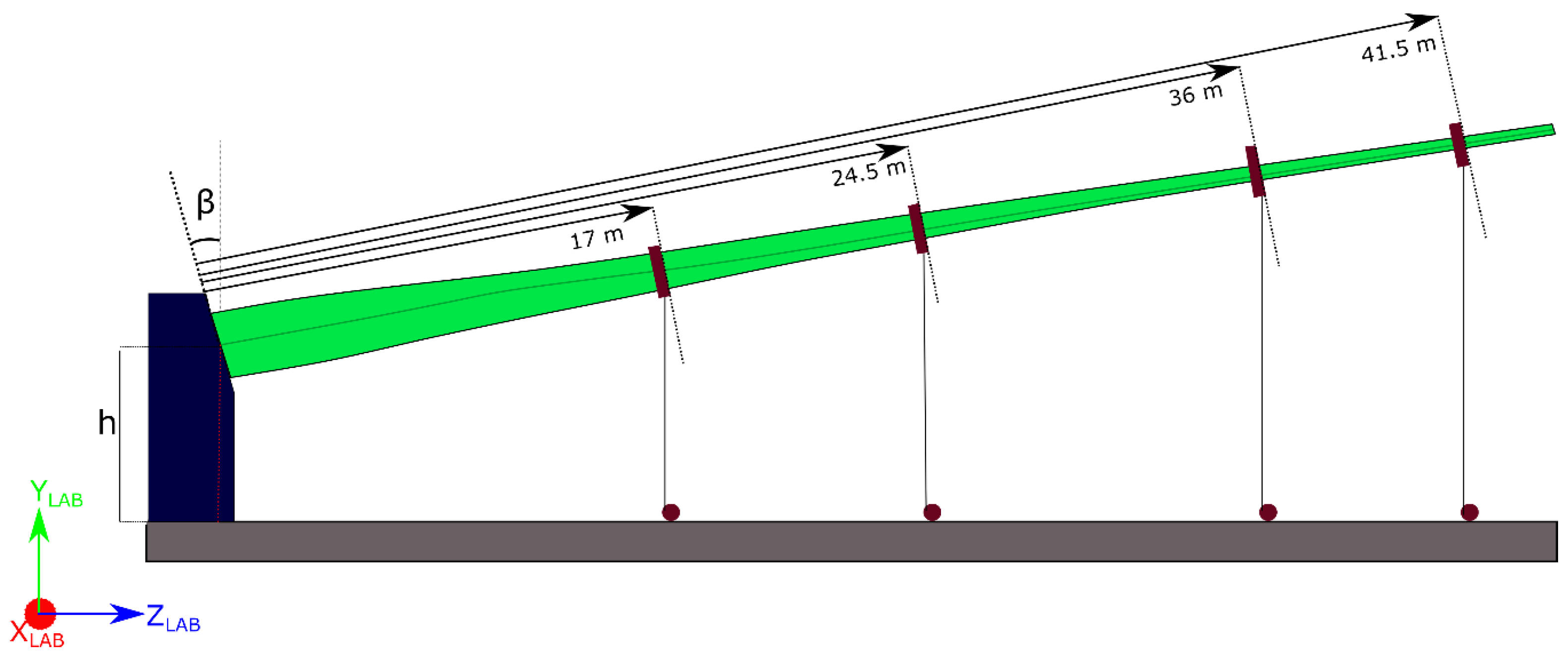
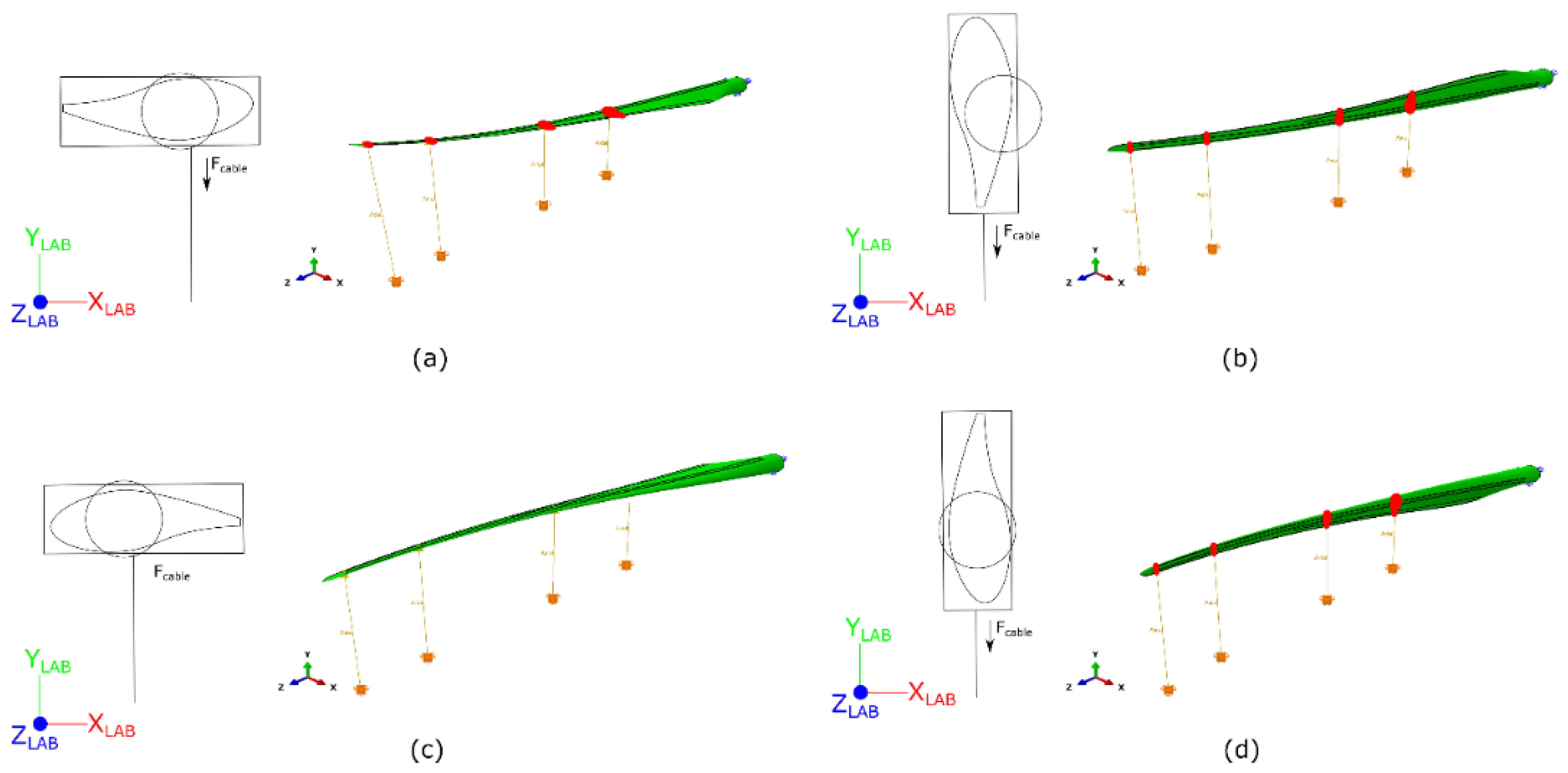
The static tests were conducted by bolting the test blade onto a reaction block using the normal T-bolt root connection. The reaction block positioned the blade at an elevation from and angle to the lab floor, as shown in Figure 1. Fixtures were then attached to the blade. These were placed at four different spanwise positions. Subsequently, cables were attached to the fixtures and connected to pulleys on the lab floor. These pulleys were positioned so that, at maximum load, the cables connecting the pulleys to the fixtures were approximately vertical. Four different load cases were experimentally tested: positive flatwise, negative flatwise, positive-edgewise, and negative edgewise. This can be seen in Figure 2. Schematic overview of the different load cases. The different loads were created by attaching the blade to the test stand at different pitch angles. (a) Blade positioned for the positive flatwise load case; (b) blade positioned for the positive edgewise load-case; (c) blade positioned for the negative flatwise load case; (d) blade positioned for the negative edgewise load case. For each test case, the loads were incremented during five subsequent steps. Between increments, the load was held constant for at least 10 s so that the load can be considered static. Meanwhile, all data from measurement equipment was recorded. This data includes: (i) the load on every individual cable; (ii) the reaction moments at the blade root; (iii) the displacement of each of the fixtures; and (iv) strains at many strain gauge locations. The longitudinal strains were measured at a series of spanwise locations on the middle of each of the girders and near the leading edge (LE) and trailing edge (TE), as well as on the shear webs. Additionally, transverse strains were measured at several locations where high strains were observed in the results of preliminary calculations.
2.3. Spar Segment
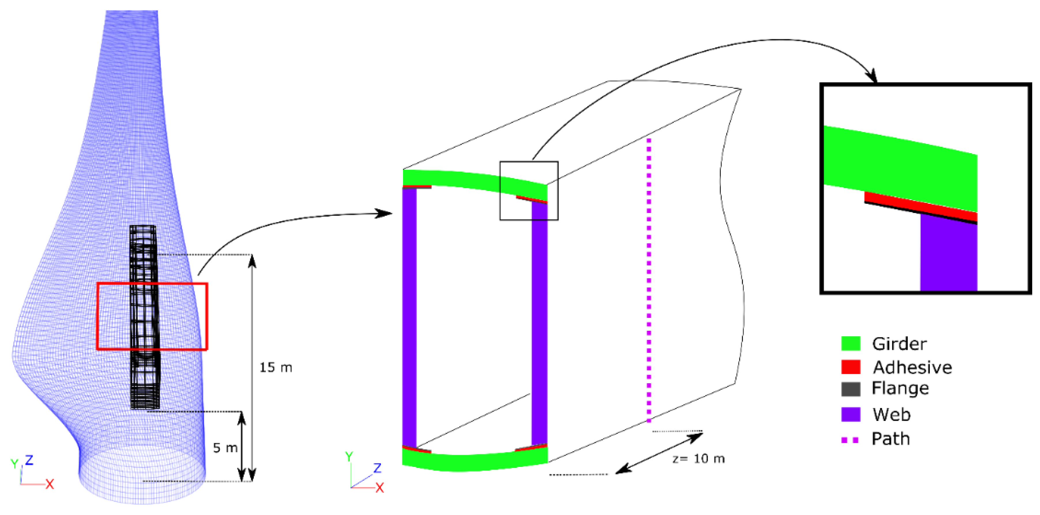
To limit the complexity, in the first step, a 10 m long portion of the blade’s spar structure was modeled. This can be seen in Figure 3. The layup of the girders was simplified in this model to consist of only unidirectional (UD) glass fiber reinforced polymer (GFRP) material. At the inboard end of the model, a multi-point constraint of the type “beam” was applied, which rigidly connected the surface to a reference node. Similarly, at the outboard end, a master node was connected to the surface, but by means of a “continuum distributing coupling”, which distributes the loads. Three different load cases were considered: pure flapwise load, combined flapwise and edgewise load, and torsion load case. An overview of the load cases can be seen in Table 1.
2.4. Full-Scale Blade
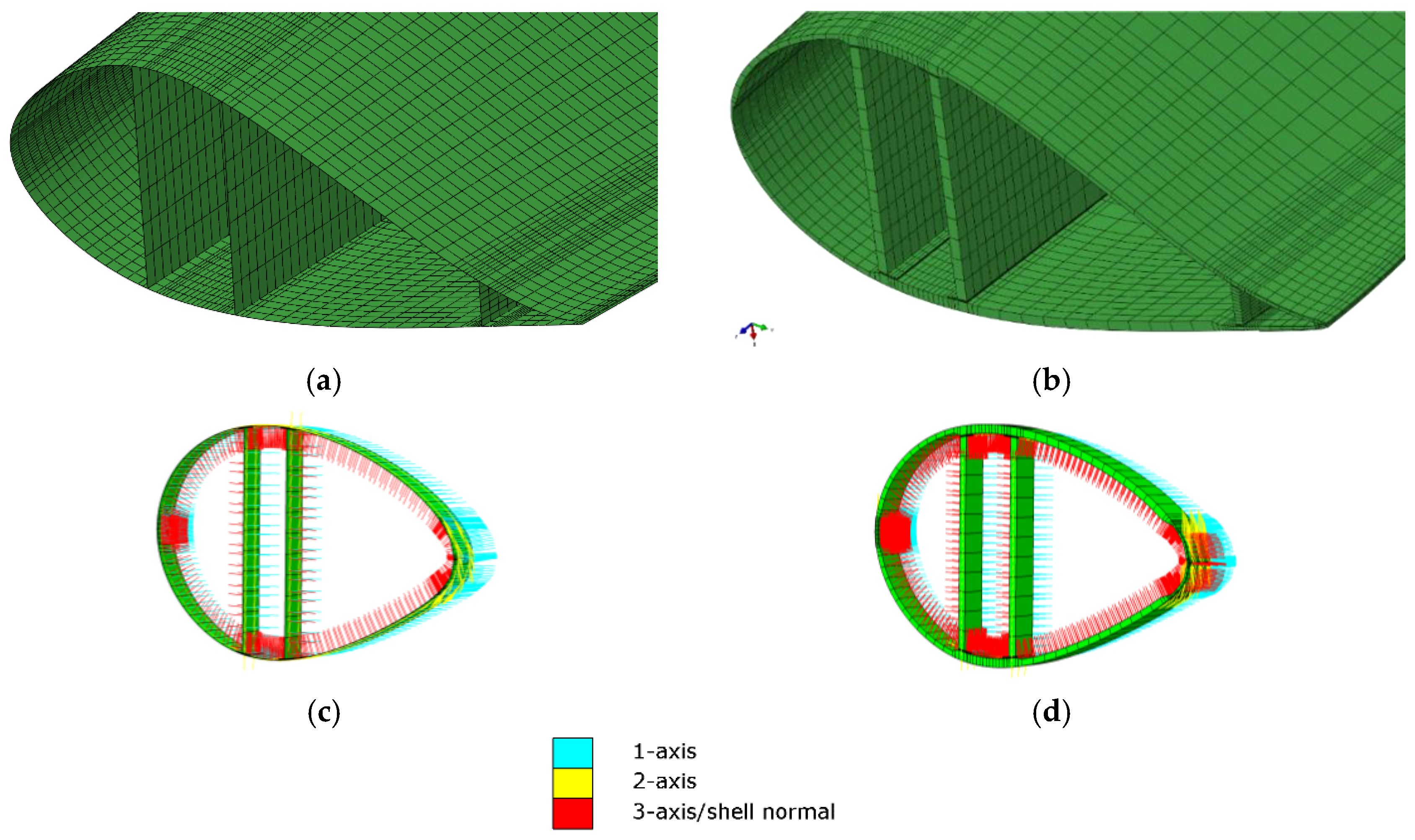
To model the full-scale blade tests, FE models of the full structure were created using an in-house developed tool. This tool enables the creation of detailed blade FE models by considering the blade as a collection of predefined parametric blocks. In this way, specific regions can be modeled by assigning the correct block. Furthermore, different models can be created from the same input. This approach differs from other tools, which are typically designed to obtain one specific type of output. The tool works by first calculating the OML shape. On this shape, functions can be defined to accurately calculate the positions of ply edges, shear webs, and adhesive bonds. These are then used to partition the blade shape, obtaining a topology onto which the layup and predefined blocks can be assigned. In this way, a wide variety of models, including those using solid elements, can be created. Furthermore, the tool is able to calculate accurate material orientations on an element-by-element basis, starting from the functions applied on the OML shape. Both a model consisting of second-order shell elements (type S8R) positioned on the OML and a model consisting of second-order layered solid elements (C3D20R) were created. Second-order shell elements are used for their transverse shear behavior. Second order solids are used to avoid locking issues. Cross-sections of these models can be seen in Figure 4. The models include accurate material orientations defined for every element individually.
Data was extracted from the simulations in an automated fashion. At the blade root, a single master node is rigidly connected to the circumference. Reaction moments and displacements were obtained from this node. Strain values were obtained from nodes at the blade OML surface. The strain values at the integration points were extrapolated to the nodal positions. For each node, the strain values were then calculated by averaging these values for the connected elements, considering only the top or bottom section point. For the longitudinal strain values on the girders, node sequences along the entire girder were used, while individual nodes were used for the other strain gauge positions.
3. Results and Discussion
3.1. Importance of Boundary Conditions and Load Introductions
First, the boundary conditions and settings for correctly modeling the static blade tests were explored. To mimic the tests as closely as possible, the models were spatially positioned to match the position of the blade in the laboratory (LAB) coordinate system. This can be seen in Figure 5. This is relevant since the deformation under gravity load is significant. The strain gauges used in the experiments were zeroed after the blade was positioned and was only loaded by gravity.
As mentioned, at the blade root connection, an MPC was used to rigidly connect all nodes to a single central master node, which results in the displacements and rotations being fully constrained. This allows simple extraction of the root bending moment and mimics the behavior of the T-bolt root connection, which prevents both displacement and rotation.
At the different load introduction positions, a master node was connected to a portion of the blade by means of a distributing coupling. This connection spreads the load of the master node over the slave nodes, without preventing deformation of the cross-section. As mentioned, cables were used to introduce the loads in the experimental tests. This means that the orientation of the force acting on the blade fixture depends on the deformation of the blade. To include this nonlinear load introduction, the cables were modeled by means of axial connector elements. Applying a connector force to these elements results in a concentrated force pointing from one end to the other end of the connector, thereby mimicking the cable. Such an approach was also used in Haselbach [18].
3.1.1. Importance of Geometric Nonlinearity
Several authors have demonstrated the need for the use of nonlinear geometry. Both options were applied to the conventional shell model. The resulting blade deformation differs significantly, as can be seen in Figure 6. This proves the need to use nonlinear geometry.
3.1.2. The Influence of the Cables
To study the effect of modeling the cables used for introducing the loads, the axial connector elements were replaced by concentrated forces along the LAB y-direction. These do not follow the rotation of the master node, but stay aligned with the y-direction. It is found that the difference in results is very limited. One exception is that the observed resulting root bending moment is slightly higher with the concentrated forces. This is not entirely unexpected since, at full load, most cables are approximately, but not perfectly, vertical and therefore introduce a load very similar to the concentrated forces.
3.1.3. The Influence of the Coupling
In literature, it has been suggested that the clamps at the load introduction points restrict the deformation of the blade cross-section and thereby influence the test. To investigate this aspect, the fixture’s distributing couplings were replaced by MPCs of the type “beam”, preventing deformation of the section. The results can be seen in Figure 7. It is clear that in the area of the fixtures, the transverse strains are forced to remain zero. However, strains at the locations with strain gauges do not show significant difference. It is worth mentioning that the position of the clamps was chosen based on the structural layup. Areas which are deemed critical to the design or which contain rapid changes in layup were typically avoided.
3.2. Comparison of Shell and Solid Models: Spar Segment
To ensure validity in comparing the OML shell and solid models, the mass and center of gravity (COG) of both models were compared. It was found that these differ less than 1%. In a subsequent step, mesh refinement analysis was conducted. Different mesh densities are produced and the displacement of the master node, as well as strains along the top of the girders, were extracted and compared. This was done separately for the lengthwise and chordwise densities, as well as for the seeding in the spar’s height direction for the webs, adhesive, and girders. From the results, it became apparent that the coarsest version of the mesh in longitudinal and chordwise directions, an average size of 100 mm, was sufficient. Furthermore, the shear web mesh was found to be sufficiently refined, with only two second-order elements over the height.
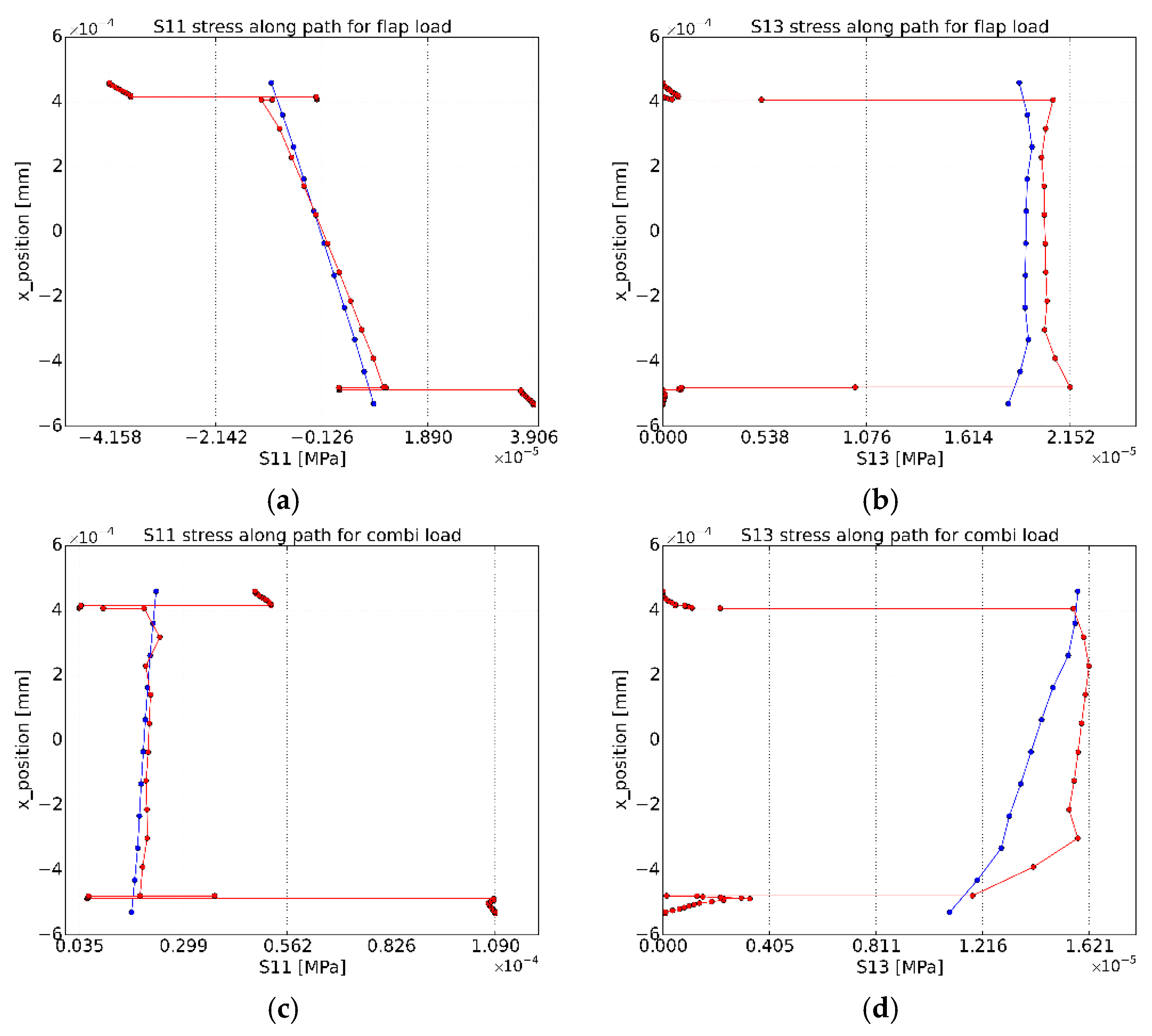
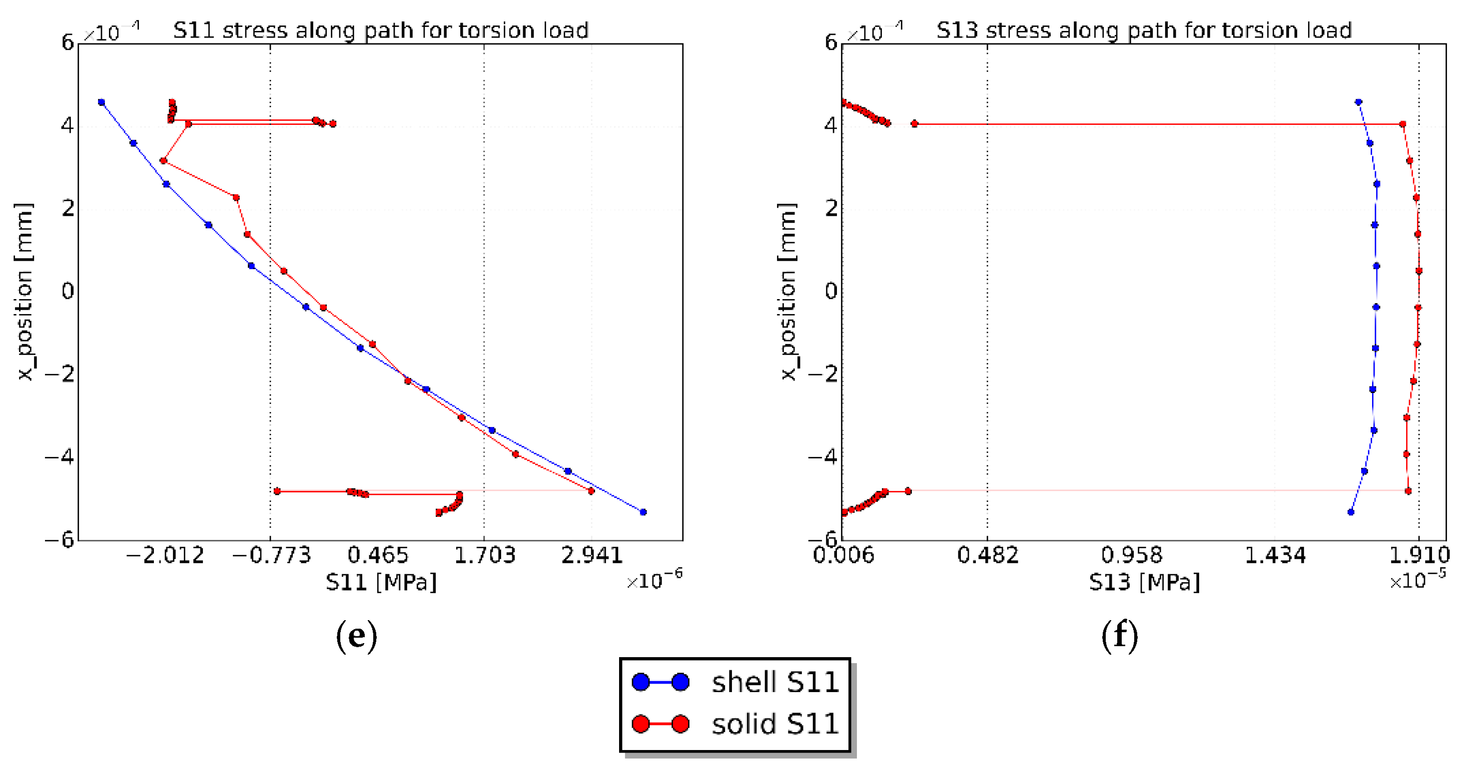
If we compare the displacements and rotations of the tip end master node, we notice that the absolute differences are very limited. This means that the overall stiffness of the structure is accurately modeled using the OML shell approach. However, some differences appear when we compare the stress values along a path on the side of the spar at the half-length position, shown in Figure 3. In the resulting graphs, plotted in Figure 8, the presence of the adhesive bond and girders becomes apparent in the solid models, while the side wall of the OML shell model does not contain these features.
The reason the OML shell model results in accurate results, despite not modeling the web joint accurately, could be that the shear stiffness resulting from the girder, adhesive, and flange (included in the solid model but not in the OML shell model) is compensated by the shear stiffness resulting from the excessive size of the shear webs in the OML shell model.
To investigate this more accurately, the girder was also modeled using an OML shell approach with the adhesive bonds represented by solid elements in contact with the outer shape. The resulting model was found to have a lower stiffness, resulting in a larger tip deflection, which differs from both the pure shell and solid models. It can therefore be concluded that this naive approach, which is employed in several works, should not be used.
3.3. Comparison of Shell and Solid Models: Full-Scale Blade
3.3.1. Validation of the Models
In this paragraph, the results of full-scale blade analyses are discussed. However, the models were first validated by comparing the total blade mass and center of gravity (COG) of the models to that of the test blade. This is shown in Table 2. The design includes T-bolts for a total of 200 kg. These are not included in the models, since their mass does not have a significant effect on the bending load.
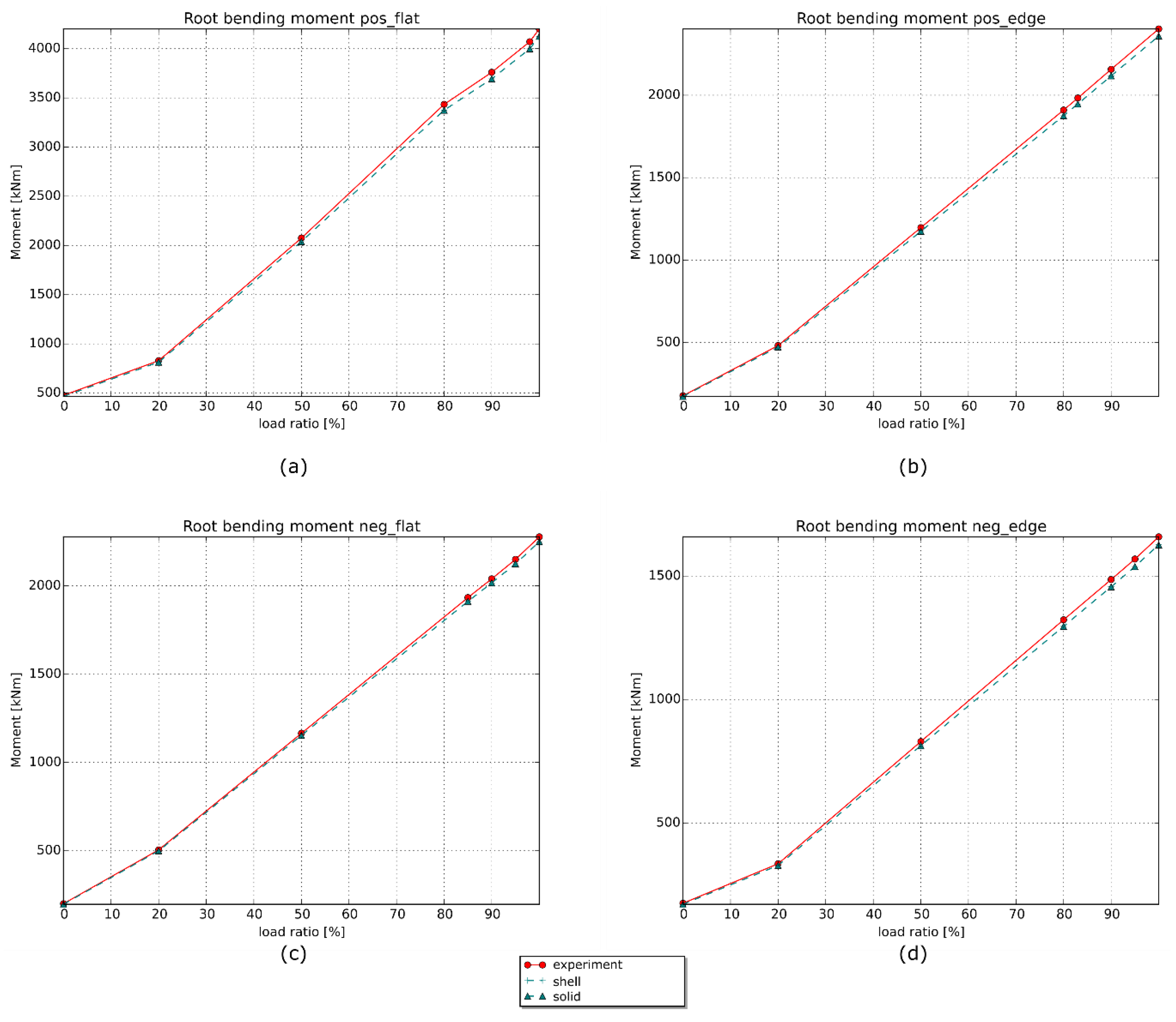
Next, the applied loads were validated. As mentioned, the magnitude of the applied connector loads is based on measured load cell values during the actual experimental tests. The resulting root bending moment is therefore compared to the measured values, as can be seen in Figure 9. This shows good similarity for each of the different load cases.
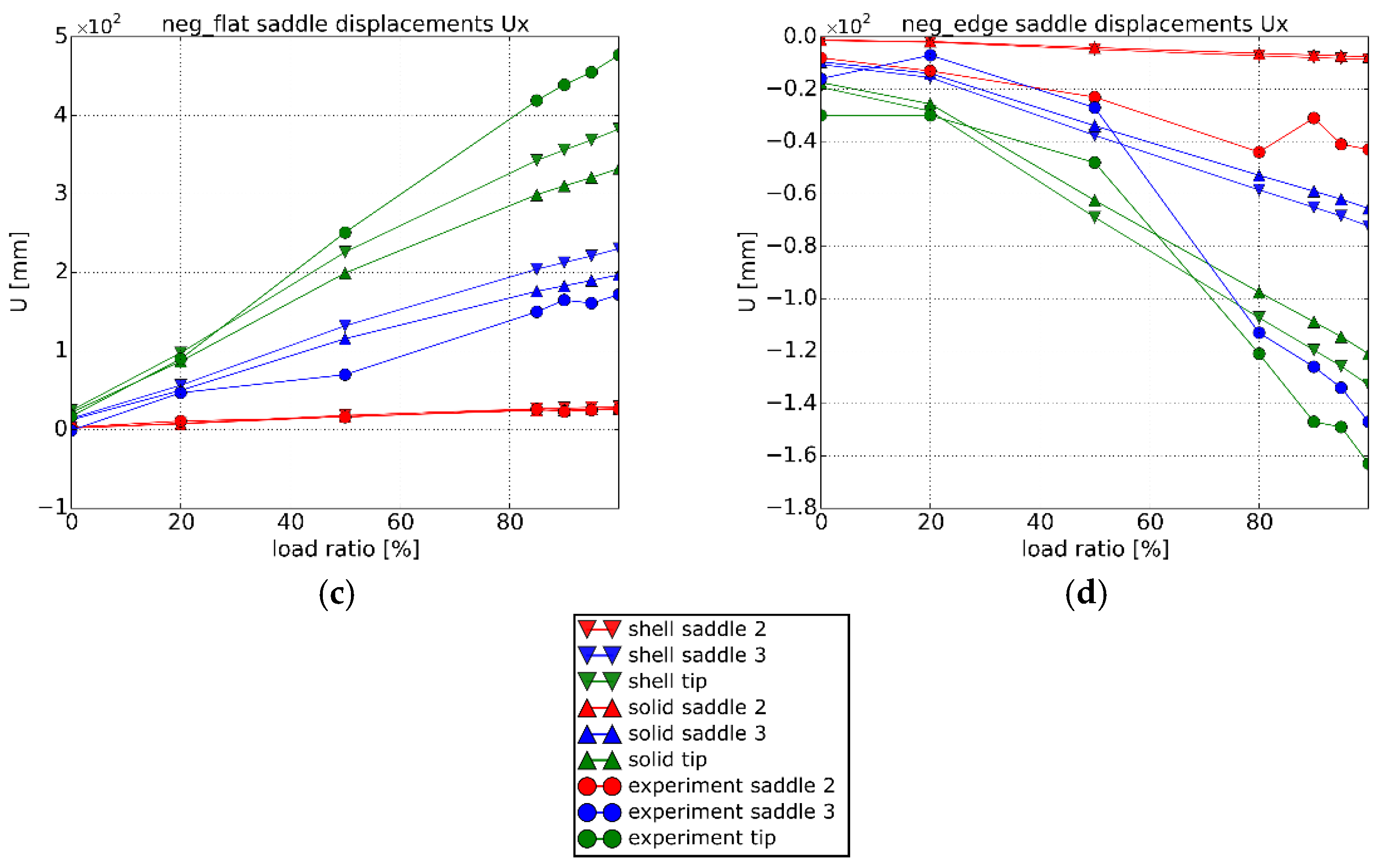
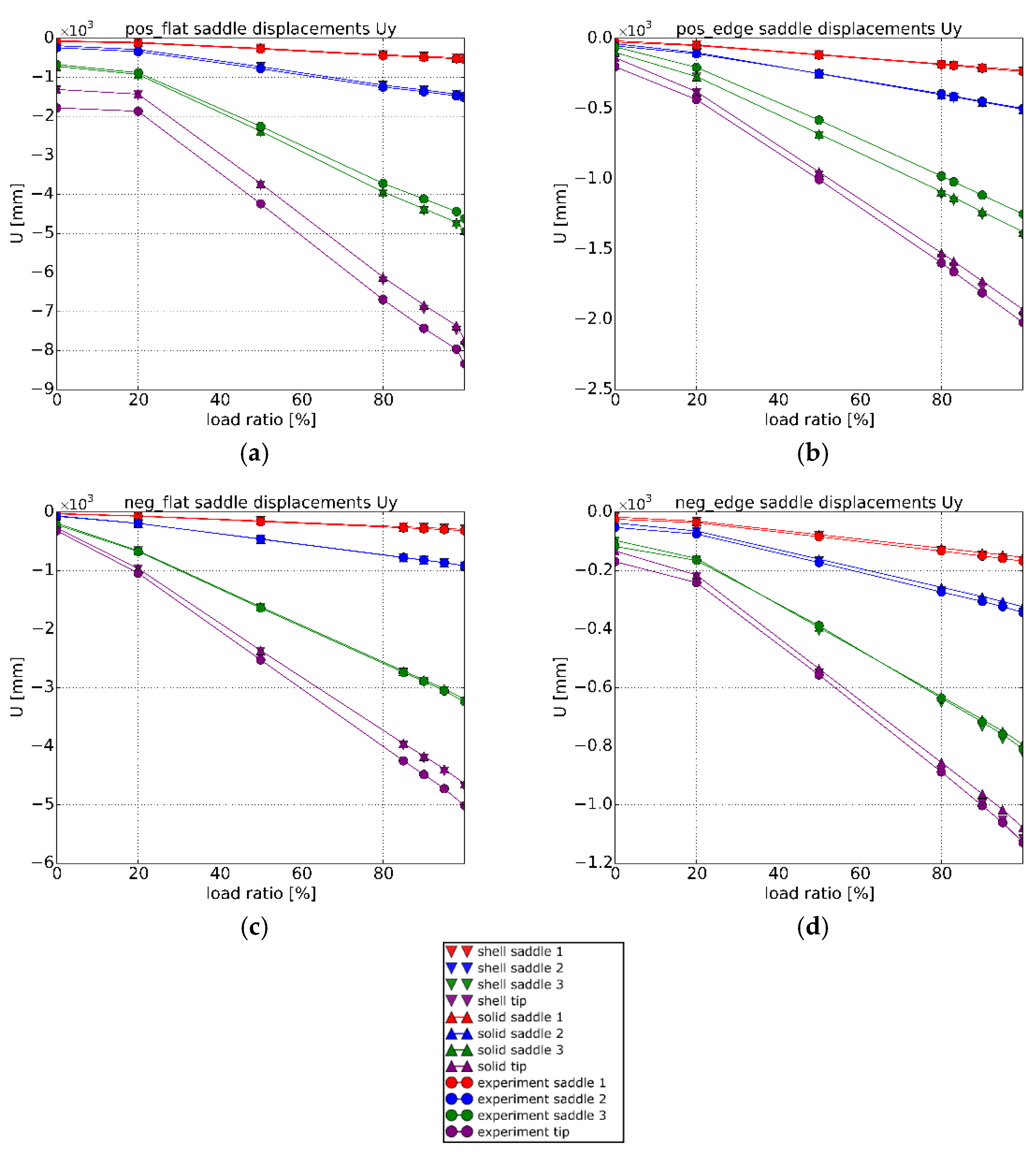
3.3.2. Fixture Displacements
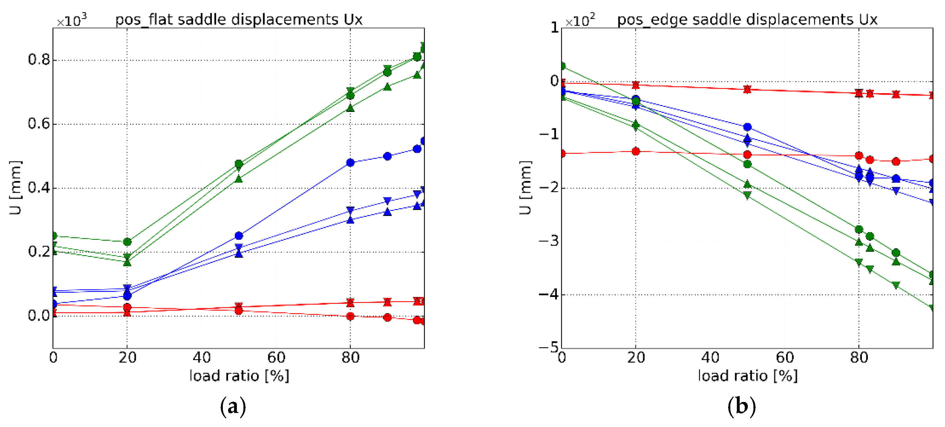
Subsequently, the displacements of the master nodes of the fixtures were extracted and compared to the measured values. These are shown in Figure 10 and Figure 11. The shell and solid models provide very similar displacements. Some differences can be observed between the measured and predicted values. These appear most pronounced in the LAB x-direction. However, the absolute values of these displacements are very small.
3.3.3. Longitudinal Strain Values
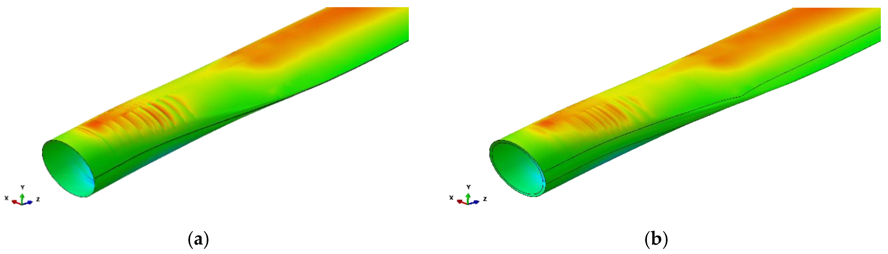
Longitudinal strain values were measured during the static tests, and data from paths on the mesh was extracted to allow comparison, as presented in Figure 12. The data shows a rather good match for both the shell and solid models. While very slight discrepancies between both modeling approaches are present, it is not clear which method provides more accurate results. In Figure 13, contour plots of the longitudinal strain under the negative flatwise load case are displayed. While both plots show a very similar image, more rapid changes in strain value can be observed in the shell model. This can be explained by the fact that the solid model has a continuous thickness, with gradual transitions, whereas in the shell model, the thickness changes are instant.
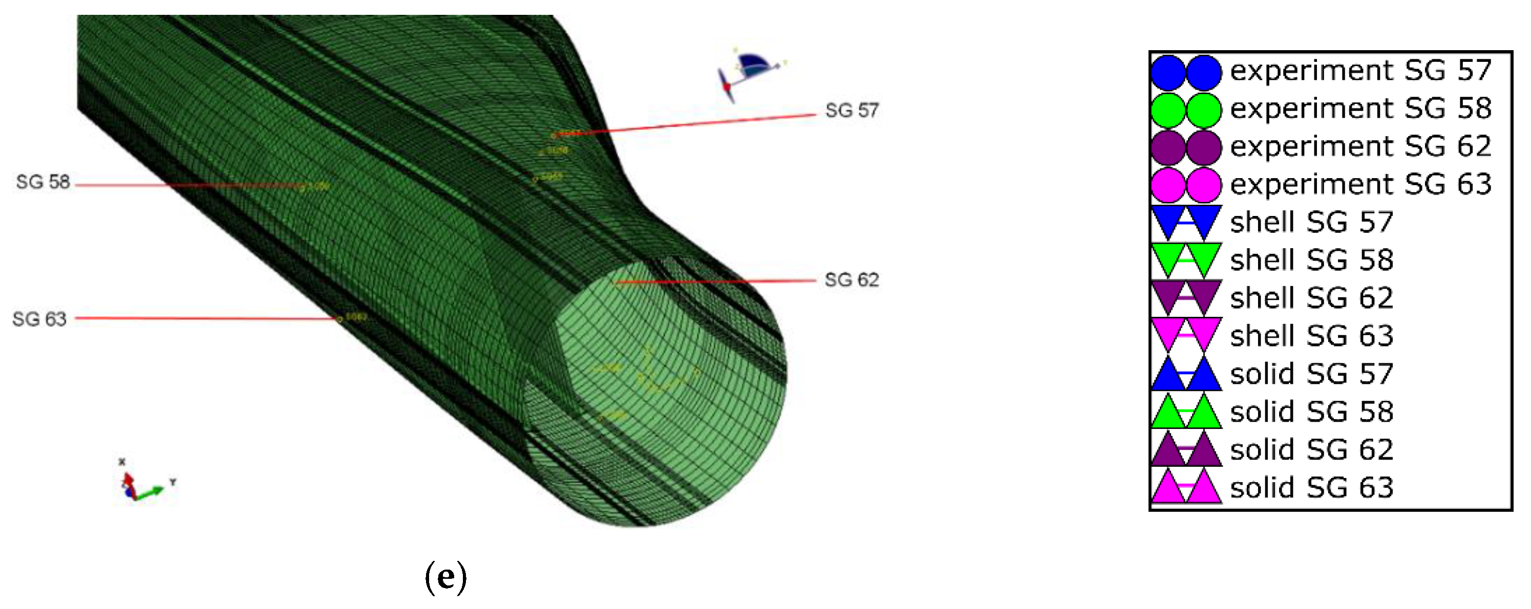
3.3.4. Transverse Strain Values
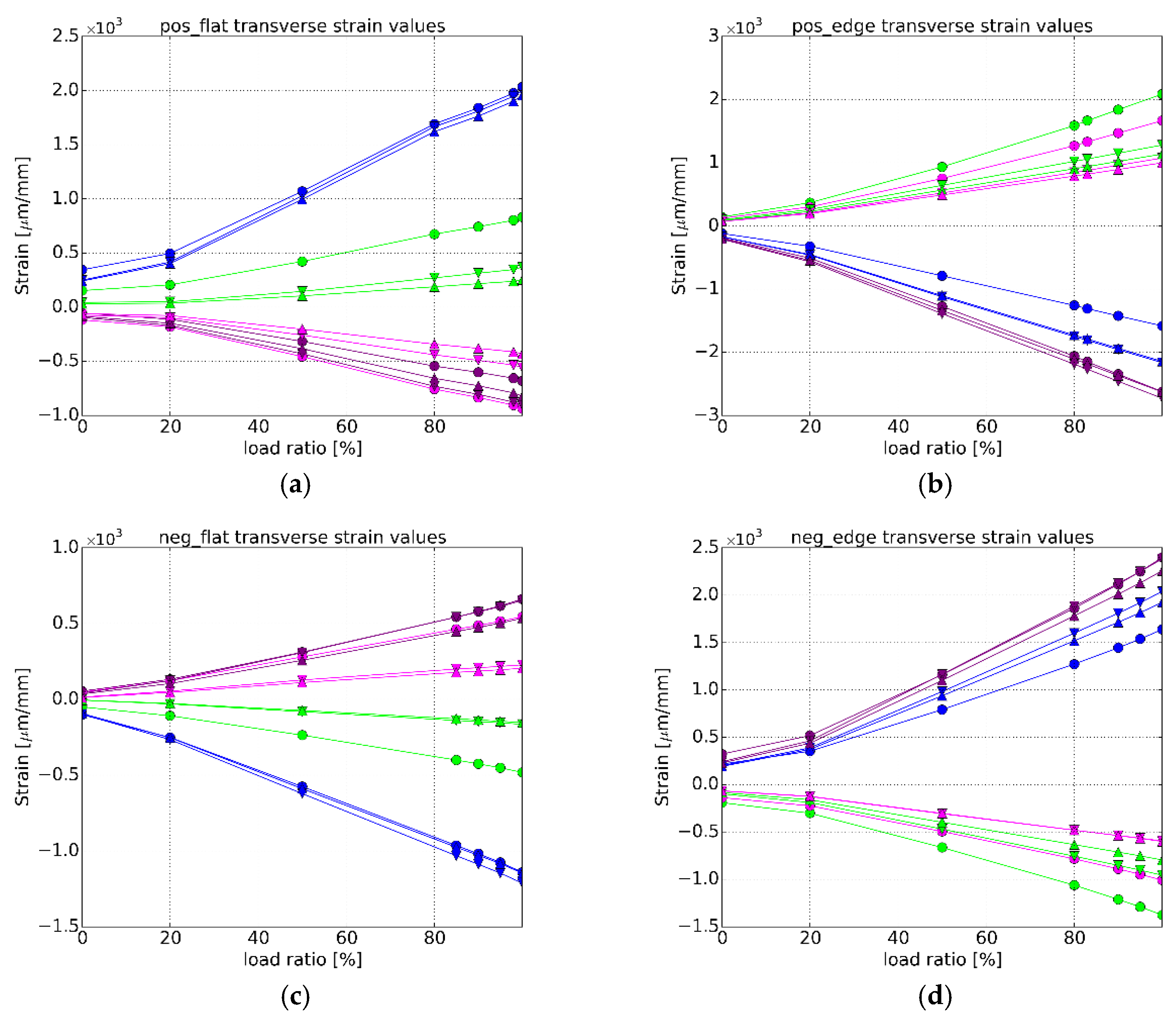
Furthermore, strain values were measured in the transverse direction. These were compared to the values obtained at the same locations in the models. The strain values were found to be very large in some regions. This can be attributed to large nonlinear deformations of the cross-section. Figure 14 shows strain values for the different load cases. Some differences between the results obtained from shell and solid modeling can be observed. In general, the differences between the shell and solid models are limited. Furthermore, the strains observed in the actual tests are larger than those observed in the simulations. In Figure 15, contour plots of the transverse strain values are shown for both the shell and solid model. Hot spots are visible in the transition zone next to the main girder.
In Figure 15, contour plots of the transverse strains are shown for the negative flatwise load case. A nearly identical strain distribution is observed. Again, slightly more gradual changes are visible in the solid model compared to the shell model, due to the gradual thickness transition inherent to the solid model.
3.3.5. Strain Differences between the Inner and Outer Surfaces
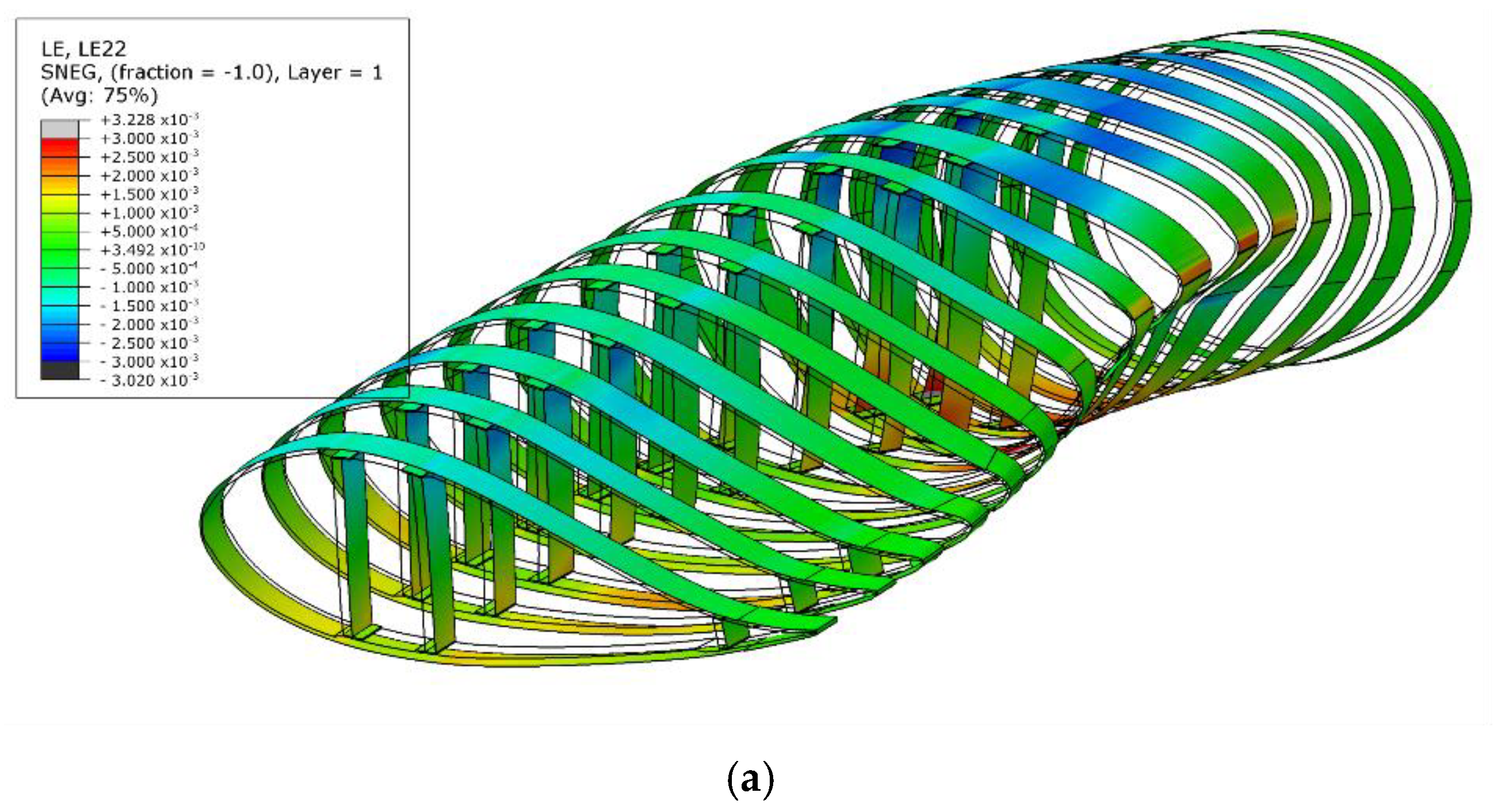
In both the experiments and simulations, significant differences are observed between the strain on the inside and outside surface at several locations on the blade. At two positions, strain gauges measuring transverse strain were placed on the in- and outside of the blade. Differences of over 1500 µm/mm are observed. These differences result in a local rotation within the surface. In Figure 16, the deformation of several blade cross-sections is shown, magnified by a factor of 20. Strain differences between inside and outside surface result in local rotations. These are related to changes in thickness and layup, as suggested in Jensen [28], and nonlinear deformation of the structure, such as the flattening of the cross-section due to the Brazier effect.
3.3.6. Computational Effort
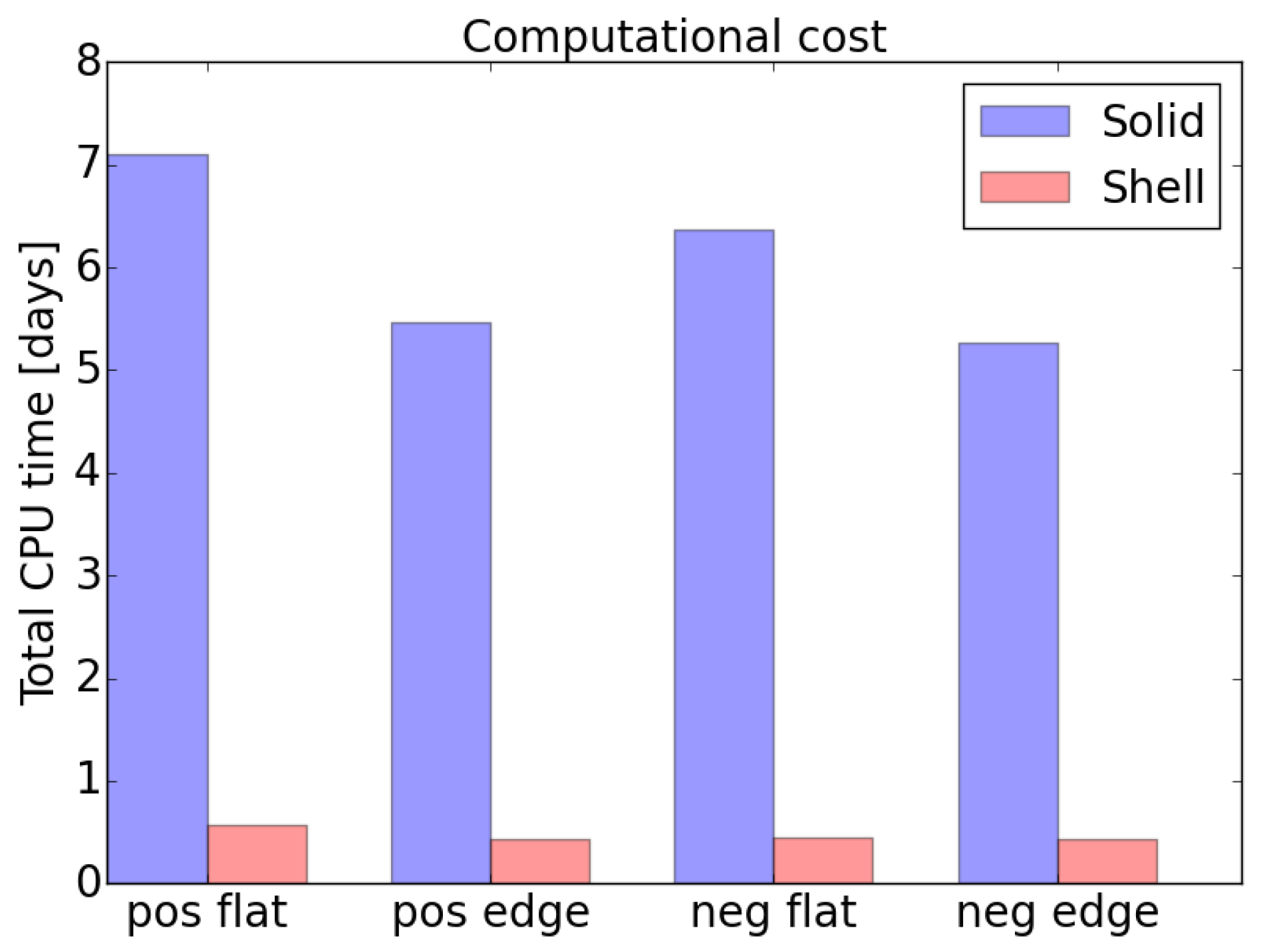
While the observed displacements and strain distributions are very similar between the shell and solid models, the computational effort for the solid model is considerably higher. In Figure 17, the total CPU times are presented for the different load cases and models. The CPU time needed for the analyses using shell models was about 10% of those using solid models. Furthermore, generating the final models with the in-house software took 4.9 min for the shell model and 22.7 min for the solid model.
3.4. Modeling Assumptions and Implications
In the blade models, several assumptions were used. Firstly, the models represent an idealized, flawless structure. The experimentally tested sample was produced under factory conditions, where manufacturing tolerances apply and flaws and defects occur. Furthermore, the models represent the blade design with the assumptions that the composite materials have the exact mechanical properties that were assumed during the design and that these properties do not vary within the structure. In addition, it was assumed that the blade did not sustain any damage throughout the tests and that the sequence in which the load cases were applied does not influence the results. These assumptions may explain some of the discrepancies between the results obtained from the models and experiments.
4. Conclusions
A commercial 43 m blade was statically tested. These tests were successfully modeled using FEM.
First, different options for modeling the static tests were investigated. It was observed that the use of geometric nonlinearity is a necessity. Furthermore, different methods of load introduction were considered. Connector elements that accurately represent the cables were compared to the use of concentrated forces. While the latter do not account for the change in orientation of the applied force as the blade deforms, the influence on the observed results was limited due to the design of the test. Furthermore, the load from the cable was spread to a spanwise region by a “flexible” distributing coupling and by a “rigid” MPC. While it was found that the MPC prevented cross-sectional deformation, resulting in transverse strain values remaining zero in the region of the clamp, its influence was found to be restricted to the vicinity of the fixtures.
Subsequently, the use of shell and solid modeling was compared. In a first approach, only a segment of the spar structure was analyzed. To this extent, a conventional OML shell model, as well as a second-order layered solid model, were produced using an in-house tool. Despite the geometric mismatch between the OML shell model and reality, the predicted stresses along the side of the spar show similar values for the shear web. It can be argued that the overall behavior of the structure is accurately predicted because the shear stiffness of the shear web is close to the transverse shear stiffness of the girder combined with the adhesive bonds and flanges. In other words, the transverse shear deformation that takes place in the girder, adhesive, and flange appears to be accounted for by the over-dimensioned shear web. Next, both a conventional OML shell model and a layered solid model were constructed for the full-scale blade. The obtained displacements and longitudinal strains are in good agreement with the experimental tests, and little difference is observed between the shell and solid models.
The OML shell models were found to be both efficient and accurate. Layered solid models did not appear to provide big differences in the prediction of strains or displacements. It can therefore be concluded that for the considered blade and load cases, the solid model provides little additional value over a conventional OML shell model. However, since the study was applied to a specific commercial blade under specific load cases, the similarity between the results obtained using shell and solid models may not be present for other blades or other, more severe, load cases. The results merely indicate that shell and solid models can be constructed and analyzed, resulting in a rather good match with experimental values. In addition, the results indicate that, in many cases, the shell modeling approach provides realistic results.
However, the use of solid elements is useful to obtain an accurate stress distribution in the adhesive bonds. Furthermore, several authors have successfully used solid models in load cases where damaged developed. In such cases, the stress in the thickness direction of the laminate is of great importance, since it results in delamination and crack growth. The assumptions inherent to a shell model do not allow for these stresses to be observed. Further, a solid model proves useful when using a submodeling approach to investigate a specific area of interest. A submodel contains multiple nodes in the laminate’s thickness direction. This allows for more accurate submodeling boundary conditions to be transmitted to the local solid model.
Author Contributions
Investigation, M.P.; Methodology, G.S.; Supervision, W.V.P.; Writing—original draft, M.P.; Writing—review & editing, J.D. and W.V.P.
Funding
The work leading to this publication has been supported by VLAIO (Flemish Government Agency for Innovation and Entrepeneurship) under the SBO project “OptiWind: Serviceability optimisation of the next generation offshore wind turbines” (project No. 120029) and “FWO-project G030414N-Fluid-structure interaction simulations of wind turbines with composite blades”.
Conflicts of Interest
The authors declare no conflict of interest. The founding sponsors had no role in the design of the study; in the collection, analyses, or interpretation of data; in the writing of the manuscript, and in the decision to publish the results.
References
- Meet LM 88.4 P—The world’s Longest Wind Turbine Blade. Available online: https://www.lmwindpower.com/en/products-and-services/blade-types/longest-blade-in-the-world (accessed on 6 March 2018).
- Caduff, M.; Huijbregts, M.A.J.; Althaus, H.-J.; Koehler, A.; Hellweg, S. Wind Power Electricity: The Bigger the Turbine, The Greener the Electricity? Environ. Sci. Technol. 2012, 46, 4725–4733. [Google Scholar] [CrossRef] [PubMed]
- Griffin, D.A. WindPACT Turbine Design Scaling Studies Technical Area 1-Composite Blades for 80- to 120-Meter Rotor; National Renewable Energy Laboratory (NREL): Golden, CO, USA, 2001.
- Sieros, G.; Chaviaropoulos, P.; Sørensen, J.D.; Bulder, B.H.; Jamieson, P. Upscaling wind turbines: Theoretical and practical aspects and their impact on the cost of energy. Wind Energy 2012, 15, 3–17. [Google Scholar] [CrossRef]
- Paquette, J.A. Blade Reliability Collaborative (BRC) Update; Sandia National Laboratories (SNL-NM): Albuquerque, NM, USA, 2011.
- Sheng, S. Report on Wind Turbine Subsystem Reliability—A Survey of Various Databases; National Renewable Energy Laboratory (NREL): Golden, CO, USA, 2013.
- Nielow, D. Prüfstand für die Evaluation der Betriebsfestigkeit von Rotorblattschalensegmenten. Presented at the Rotorblätter von Windenergieanlagen—Wind Turbine Rotor Blades 6th Technical Conference, Essen, Germany, 2–3 July 2014. [Google Scholar]
- Det Norske Veritas. Design and Manufacture of Wind Turbine Blades, Offshore and Onshore Wind Turbines; Det Norske Veritas: Oslo, Norway, 2010. [Google Scholar]
- Germanischer Lloyd. Guideline for the Certification of Wind Turbines, GL-IV-1; Germanischer Lloyd: Hamburg, Germany, 2010. [Google Scholar]
- Yang, J.; Peng, C.; Xiao, J.; Zeng, J.; Yuan, Y. Application of videometric technique to deformation measurement for large-scale composite wind turbine blade. Appl. Energy 2012, 98, 292–300. [Google Scholar] [CrossRef]
- Jensen, F.M.; Falzon, B.G.; Ankersen, J.; Stang, H. Structural testing and numerical simulation of a 34 m composite wind turbine blade. Compos. Struct. 2006, 76, 52–61. [Google Scholar] [CrossRef]
- Rosemeier, M.; Berring, P.; Branner, K. Non-linear ultimate strength and stability limit state analysis of a wind turbine blade: Non-linear ultimate strength and stability limit state analysis of a wind turbine blade. Wind Energy 2016, 19, 825–846. [Google Scholar] [CrossRef]
- Kim, S.-H.; Bang, H.-J.; Shin, H.-K.; Jang, M.-S. Composite Structural Analysis of Flat-Back Shaped Blade for Multi-MW Class Wind Turbine. Appl. Compos. Mater. 2014, 21, 525–539. [Google Scholar] [CrossRef]
- Yang, J.; Peng, C.; Xiao, J.; Zeng, J.; Xing, S.; Jin, J.; Deng, H. Structural investigation of composite wind turbine blade considering structural collapse in full-scale static tests. Compos. Struct. 2013, 97, 15–29. [Google Scholar] [CrossRef]
- Laird, D.; Montoya, F.; Malcolm, D. Finite Element Modeling of Wind Turbine Blades. In Aerospace Sciences Meetings, Proceedings of the 43rd AIAA Aerospace Sciences Meeting and Exhibit, Reston, VA, USA, 10–13 January 2005; American Institute of Aeronautics and Astronautics: Reston, VA, USA, 2005. [Google Scholar]
- Ashwill, T. Sweep-Twist Adaptive Rotor Blade: Final Project Report; Sandia National Laboratories: Albuquerque, NM, USA, 2010.
- Branner, K.; Berring, P.; Berggreen, C.; Knudsen, H.W. Torsional performance of wind turbine blades—Part II: Numerical validation. In Proceedings of the 16th International Conference on Composite Materials, Kyoto, Japan, 8–13 July 2007; ICCM: Kyoto, Japan, 2007; pp. 8–13. [Google Scholar]
- Haselbach, P.U. An advanced structural trailing edge modelling method for wind turbine blades. Compos. Struct. 2017, 180, 521–530. [Google Scholar] [CrossRef]
- Wetzel, K.K. Defect-Tolerant Structural Design of Wind Turbine Blades. In Proceedings of the 50th AIAA/ASME/ASCE/AHS/ASC Structures, Structural Dynamics, and Materials Conference, Structures, Structural Dynamics, and Materials and Co-located Conferences, Palm Springs, CA, USA, 4–7 May 2009; American Institute of Aeronautics and Astronautics: Reston, VA, USA, 2009. [Google Scholar]
- Overgaard, L.C.T.; Lund, E.; Thomsen, O.T. Structural collapse of a wind turbine blade. Part A: Static test and equivalent single layered models. Compos. Part A Appl. Sci. Manuf. 2010, 41, 257–270. [Google Scholar] [CrossRef]
- Overgaard, L.C.T.; Lund, E. Structural collapse of a wind turbine blade. Part B: Progressive interlaminar failure models. Compos. Part A Appl. Sci. Manuf. 2010, 41, 271–283. [Google Scholar] [CrossRef]
- Haselbach, P.U.; Bitsche, R.D.; Branner, K. The effect of delaminations on local buckling in wind turbine blades. Renew. Energy 2016, 85, 295–305. [Google Scholar] [CrossRef]
- Chen, X.; Zhao, W.; Zhao, X.; Xu, J. Failure Test and Finite Element Simulation of a Large Wind Turbine Composite Blade under Static Loading. Energies 2014, 7, 2274–2297. [Google Scholar] [CrossRef]
- Chen, X.; Zhao, X.; Xu, J. Revisiting the structural collapse of a 52.3 m composite wind turbine blade in a full-scale bending test: Structural collapse of a 52.3 m composite wind turbine blade. Wind Energy 2017, 20, 1111–1127. [Google Scholar] [CrossRef]
- Shah, O.R.; Tarfaoui, M. The identification of structurally sensitive zones subject to failure in a wind turbine blade using nodal displacement based finite element sub-modeling. Renew. Energy 2016, 87, 168–181. [Google Scholar] [CrossRef]
- Ji, Y.M.; Han, K.S. Fracture mechanics approach for failure of adhesive joints in wind turbine blades. Renew. Energy 2014, 65, 23–28. [Google Scholar] [CrossRef]
- Abaqus Unified FEA—SIMULIA™ by Dassault Systèmes®. Available online: https://www.3ds.com/products-services/simulia/products/abaqus/ (accessed on 11 April 2018).
- Jensen, F.M.; Stang, H.; Branner, K. Ultimate Strength of a Large Windturbine Blade; Risø-PhD, no. 34(EN); Risø National Laboratory for Sustainable Energy, Technical University of Denmark: Copenhagen, Denmark, 2009. [Google Scholar]
Figure 1.
Schematic overview of the static test setup. The blade was positioned onto the reaction block at a height (h) of approx. 4.5 m at an angle of 13 deg. The lab coordinate system was positioned as indicated. Different load cases were created by mounting the blade onto the test stand under a different pitch angle. Loads were introduced by means of four fixtures mounted on the blade at distances of 17 m, 24.5 m, 36 m, and 41.5 m from the root.

Figure 2.
Schematic overview of the different load cases. The different loads were created by attaching the blade to the test stand at different pitch angles. (a) Blade positioned for the positive flatwise load case; (b) blade positioned for the positive edgewise load-case; (c) blade positioned for the negative flatwise load case; (d) blade positioned for the negative edgewise load case.

Figure 3.
In a first approach, the model was limited to a portion of the spar; (left) spar segment in the overall blade; (middle) front view of the spar, showing the unidirectional (UD) girders, shear webs with flanges, and adhesive bonds. A path for the extraction of data from the simulations was added to the side of the model over the full height of the spar; (right) close-up view of a corner of the spar segment.

Figure 4.
Cross-sections of the different finite element (FE) models. (a) Conventional outer mold layer (OML) shell model, consisting of second-order S8R elements; (b) model consisting of second-order, layered solid elements, C3D20R; (c) slice of the OML shell model showing the local material orientations; (d) slice of the solid model showing the local material orientations.

Figure 5.
View of the full-scale models and static test setup, with the blade positioned for the negative flatwise load case. A drawing of a human is added for scale. (left) Unloaded configuration; (right) configuration at full load.
Figure 5.
View of the full-scale models and static test setup, with the blade positioned for the negative flatwise load case. A drawing of a human is added for scale. (left) Unloaded configuration; (right) configuration at full load.
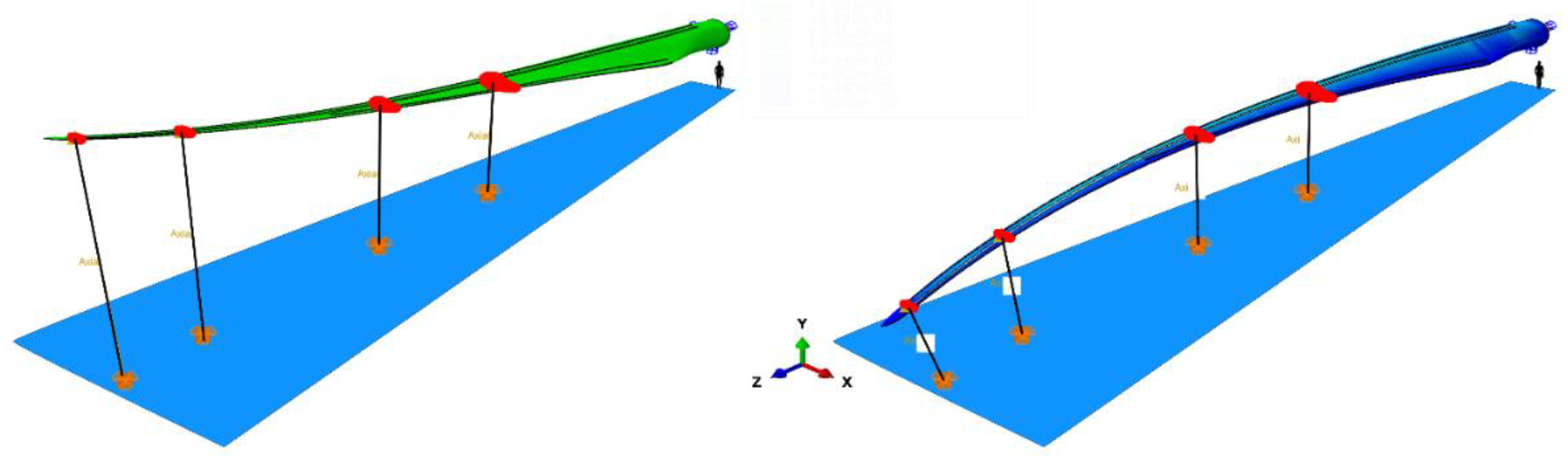
Figure 6.
Contour plots of the displacements in the z-direction of the conventional OML shell model on the deformed shape under static load. (a) The result obtained from a geometrically linear calculation; (b) the result from a geometrically nonlinear calculation.
Figure 6.
Contour plots of the displacements in the z-direction of the conventional OML shell model on the deformed shape under static load. (a) The result obtained from a geometrically linear calculation; (b) the result from a geometrically nonlinear calculation.
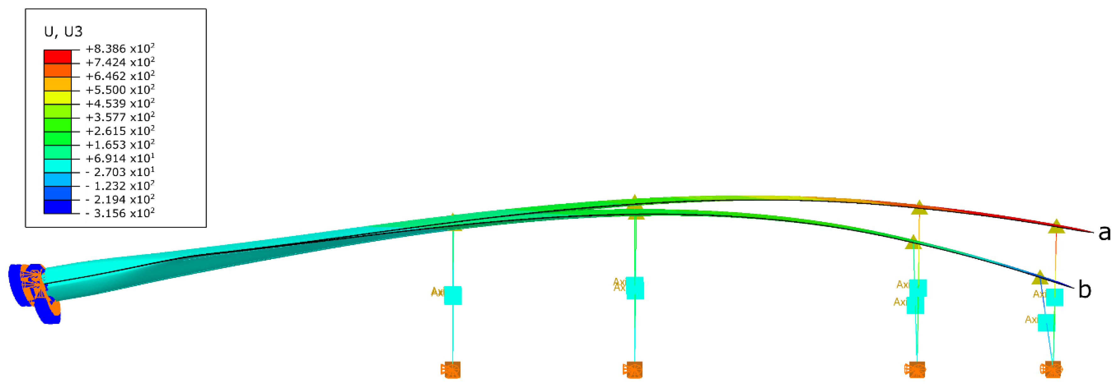
Figure 7.
Contour plots of the transverse true strain values. (a) Using a “flexible” distributing coupling; (b) using a “rigid” multi-point constraint.
Figure 7.
Contour plots of the transverse true strain values. (a) Using a “flexible” distributing coupling; (b) using a “rigid” multi-point constraint.

Figure 8.
Plots of the stress values along a path on the side of the spar model for different load cases. (a) Longitudinal stress S11 for the flapwise load case; (b) shear stress S13 for the flapwise load case; (c) longitudinal stress S11 for the combined flap and edgewise load case; (d) shear stress S13 for the combined load case; (e) longitudinal stress S11 for the torsion load case; (f) shear stress S13 for the torsion load case.


Figure 9.
Root bending moment about the x-axis in the lab coordinate system for the different load cases. (a) Positive flatwise load case; (b) positive edgewise load case; (c) negative flatwise load case; (d) negative edgewise load case.
Figure 9.
Root bending moment about the x-axis in the lab coordinate system for the different load cases. (a) Positive flatwise load case; (b) positive edgewise load case; (c) negative flatwise load case; (d) negative edgewise load case.

Figure 10.
Saddle displacements Ux for the different load cases. (a) Positive flatwise load case; (b) positive edgewise load case; (c) negative flatwise load case; (d) negative edgewise load case.
Figure 10.
Saddle displacements Ux for the different load cases. (a) Positive flatwise load case; (b) positive edgewise load case; (c) negative flatwise load case; (d) negative edgewise load case.


Figure 11.
Saddle displacements Uy for the different load cases. (a) Positive flatwise load case; (b) positive edgewise load case; (c) negative flatwise load case; (d) negative edgewise load case.
Figure 11.
Saddle displacements Uy for the different load cases. (a) Positive flatwise load case; (b) positive edgewise load case; (c) negative flatwise load case; (d) negative edgewise load case.

Figure 12.
Overview of the true strain in the longitudinal direction along the different paths. (a) Positive flatwise load case; (b) positive edgewise load case; (c) negative flatwise load case; (d) negative edgewise load case; (e) 3D plot of the path locations on the blade OML surface.
Figure 12.
Overview of the true strain in the longitudinal direction along the different paths. (a) Positive flatwise load case; (b) positive edgewise load case; (c) negative flatwise load case; (d) negative edgewise load case; (e) 3D plot of the path locations on the blade OML surface.

Figure 13.
Contour plot of the longitudinal strain on the blade under the negative flatwise load case. (a) OML shell model; (b) layered solid model.
Figure 13.
Contour plot of the longitudinal strain on the blade under the negative flatwise load case. (a) OML shell model; (b) layered solid model.

Figure 14.
Overview of the transverse true strain values at the different strain gauge locations. (a) Positive flatwise load case; (b) positive edgewise load case; (c) negative flatwise load case; (d) negative edgewise load case; (e) overview of the locations of the strain gauges.
Figure 14.
Overview of the transverse true strain values at the different strain gauge locations. (a) Positive flatwise load case; (b) positive edgewise load case; (c) negative flatwise load case; (d) negative edgewise load case; (e) overview of the locations of the strain gauges.


Figure 15.
Contour plots of the transverse strain data for the negative flatwise load case. Transverse strains are observed next to the main girder. A very similar stress distribution is obtained by the shell and solid models. (left) OML shell model; (right) layered solid model.
Figure 15.
Contour plots of the transverse strain data for the negative flatwise load case. Transverse strains are observed next to the main girder. A very similar stress distribution is obtained by the shell and solid models. (left) OML shell model; (right) layered solid model.

Figure 16.
Contour plots of the transverse true strain values on a series of cross-sections of the solid model, deformed under the negative flatwise load case. The deformation is scaled by a factor 20 for clarity. (a) Strain values on the outside surface; (b) strain values on the inside surface.
Figure 16.
Contour plots of the transverse true strain values on a series of cross-sections of the solid model, deformed under the negative flatwise load case. The deformation is scaled by a factor 20 for clarity. (a) Strain values on the outside surface; (b) strain values on the inside surface.

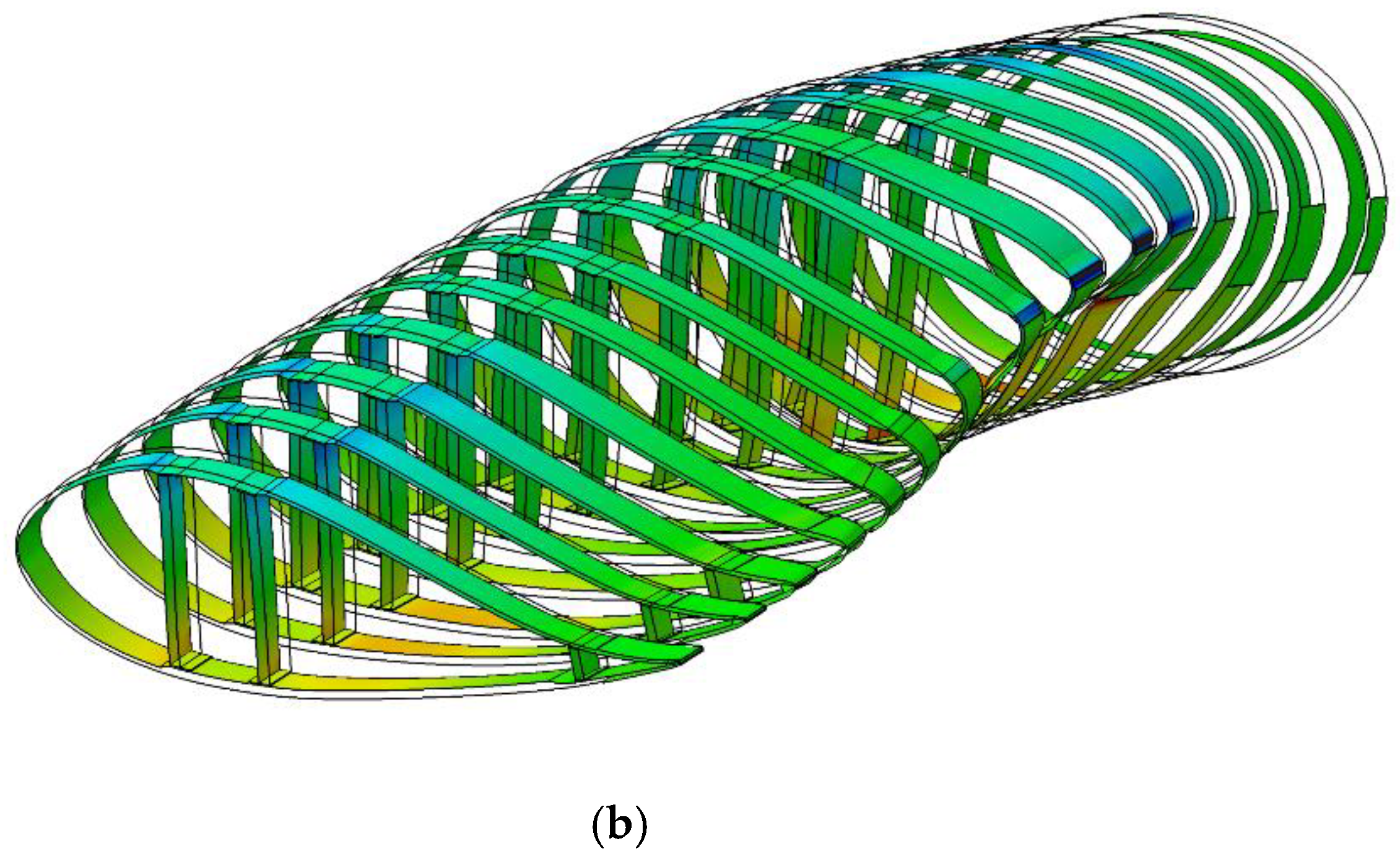
Figure 17.
Comparison between the computational costs for the different load cases for the final shell and solid models considered in this study. The CPU time required to calculate the shell models is less than 10% of that for the solid models. The analyses were parallelized over multiple CPUs.
Figure 17.
Comparison between the computational costs for the different load cases for the final shell and solid models considered in this study. The CPU time required to calculate the shell models is less than 10% of that for the solid models. The analyses were parallelized over multiple CPUs.

Table 1.
Overview of the considered load cases for the spar segment.
| Load Case | Tip Side Load | Load Magnitude |
|---|---|---|
| Flapwise | Flap-wise concentrated force Fx | 150 kN |
| Combined | Flap-wise and edge-wise concentrated force Fx, Fy | 150 kN, 50 kN |
| Torsion | Torsional moment Mz | 0.3 kNm |
Table 2.
Overview of the masses of the different models and design. The T-bolts are not included. COG: center of gravity.
Table 2.
Overview of the masses of the different models and design. The T-bolts are not included. COG: center of gravity.
| Representation | Total Mass (kg) | Spanwise Position COG (m) |
|---|---|---|
| Design excl. T-bolts | 6150 | 13.7 |
| Classic OML shell model | 6240 | 13.5 |
| OML shell model with adhesive | 6120 | 13.6 |
| Solid model | 6180 | 13.5 |
© 2018 by the authors. Licensee MDPI, Basel, Switzerland. This article is an open access article distributed under the terms and conditions of the Creative Commons Attribution (CC BY) license (http://creativecommons.org/licenses/by/4.0/).
Share and Cite
MDPI and ACS Style
Peeters, M.; Santo, G.; Degroote, J.; Van Paepegem, W. Comparison of Shell and Solid Finite Element Models for the Static Certification Tests of a 43 m Wind Turbine Blade. Energies 2018, 11, 1346. https://doi.org/10.3390/en11061346
AMA Style
Peeters M, Santo G, Degroote J, Van Paepegem W. Comparison of Shell and Solid Finite Element Models for the Static Certification Tests of a 43 m Wind Turbine Blade. Energies. 2018; 11(6):1346. https://doi.org/10.3390/en11061346
Chicago/Turabian StylePeeters, Mathijs, Gilberto Santo, Joris Degroote, and Wim Van Paepegem. 2018. "Comparison of Shell and Solid Finite Element Models for the Static Certification Tests of a 43 m Wind Turbine Blade" Energies 11, no. 6: 1346. https://doi.org/10.3390/en11061346
Note that from the first issue of 2016, this journal uses article numbers instead of page numbers. See further details here.