Electricity Price Forecasting with Dynamic Trees: A Benchmark Against the Random Forest Approach

Abstract

Dynamic Trees are a tree-based machine learning technique specially designed for online environments where data are to be analyzed sequentially as they arrive. Our purpose is to test this methodology for the very first time for Electricity Price Forecasting (EPF) by using data from the Iberian market. For benchmarking the results, we will compare them against another tree-based technique, Random Forest, a widely used method that has proven its good results in many fields. The benchmark includes several versions of the Dynamic Trees approach for a very short term EPF (one-hour ahead) and also a short term (one-day ahead) approach but only with the best versions. The numerical results show that Dynamic Trees are an adequate method, both for very short and short term EPF—even improving upon the performance of the Random Forest method. The comparison with other studies for the Iberian market suggests that Dynamic Trees is a proper and promising method for EPF.

1. Introduction

Electricity has become an indispensable commodity for all societies. Commonly, its price is traded in a market in which, due to the deregulation process and the existence of competitive markets, the price of electric power fluctuates according to consumer demand and the offers of the different producers, so the prediction of that price has become a need, not only for energy companies (such as producers, power transmission operators and retailers) but also for all kinds of market participants (such as investors or traders) and, of course, the final consumers. Due to the complexity of operation of this market, with its high volatility and price spikes, Electricity Price Forecasting (EPF) has been approached from several different viewpoints and, nowadays, it is still an open research field [1,2] in which new formulas are sought to improve the predictions.

Among the wide variety of existing methods, our study is focused in methods where the approach to the EPF problem has a statistical basis and, specifically, to machine learning techniques (sometimes called “computational intelligence” techniques). Artificial Neural Networks (ANN) [3] is an extensively used technique for this problem [4], providing accurate results—for an in-depth review of its applications, readers may consult [1,2,5]. Support Vector Machines (SVM) [6], sometimes called Support Vector Regression in this area due to the fact that its application here is for a regression problem, are also widely used [7] and provide very good results—see [1,2] for a thorough review. Tree-based techniques are also used, and from among these tree-based techniques, and due to its accuracy and reliability in all kinds of applications and not only EPF, Random Forests (RF) [8] are specially used [9,10].

In our work we want to use a machine learning technique that, as far as we know, has never been used to face this problem, the so-called Dynamic Trees [11]. Dynamic Trees are sequential regression trees based in the classical Bayesian Trees models [12] but especially useful for online processes (sometimes called “data streams”) where data are received in sequential order as they become available—as, in fact, happens during hourly clearing price forecasting. Due to the fact that Dynamic Trees are designed to work in online environments, its approach to the problem of forecasting differs from those ANN, SVM or RF as the nature of these three last techniques forces them to work in batch mode, that is, each time we want to forecast we have to train a whole new model with previously available training data. However, Dynamic Trees work in online mode as they use an active learning strategy where sequential algorithms are used for choosing input data at which output data are assembled for model fitting, that is, the same model is updated with the arrival of new available data by using a criterion that tries to minimize the forecasting errors. We must note that the purpose of our research is to find out if Dynamic Trees are a suitable technique for the EPF problem and if they are able to provide accurate forecasts. That is why we are going to use the technique in its pure form, as it was designed, for finding out if we must discount it in future studies or if on the contrary, it can be considered as a useful technique in such studies.

Because of the above, we are not going to use more sophisticated or elaborated strategies or techniques for forecasting. For example: we are going to use un-preprocessed data, that is, we are not going to study the data before our forecast looking for combinations of the variables that may reduce the complexity of the problem, like Principal Component Analysis [13] or Independent Component Analysis [14] algorithms can do. We are also not going to study our problem in the frequency domain like Wavelets do [15], and we are not going to filter the data with some reasonable criteria for price spike detection before using forecasting techniques on the filtered data [16]. All these, and many more, are typical approximations to the EPF problem that provide good results, specially when combined with other machine learning techniques [17,18,19,20,21,22,23], but, again, we just want to know if the raw Dynamic Trees technique, used as-is, is a good one in this area.

That is why we have designed a very simple test. Using data from the Iberian market, we shall divide the data into two sets, a training set and a test set, and, after training with Dynamic Trees, we shall forecast the electricity prices for the test set. First of all, we shall make a very short term forecast, trying to forecast one-hour ahead prices by using the several available versions of Dynamic Trees and looking for understanding the behavior of this technique when facing an EPF problem and then finding the best strategy of all the proven versions. Then we shall use this best strategy to forecast one-day (24 h) ahead prices, a more useful kind of forecast for market applications. However, if we want to know its accuracy in EPF, we must compare our results for the same period and for the same variables with the forecasts provided by others technique—that is why we have chosen Random Forests, with also a tree-based nature, which has proven its reliability in several real-world prediction task fields. Once again we must remember that our purpose is to determine the possibility of using this technique in additional studies—should we finally determine its utility. If the results are good enough, further studies should be done comparing the results with other techniques such as, for instance, ANN or SVM. In the next sections we shall describe the tests performed with the two machine learning methodologies and we shall discuss the results obtained.

2. Dataset

We are going to use data from the Spanish electricity market, available thanks to the Iberian Energy Market Operator (OMIE). We must remark that the Spanish market is considered especially difficult to forecast due to the non-stationary mean and variance, the multiple and complex seasonality, the high volatility of prices and the high proportion of outliers [24].

In our study we have hourly data of the most important explanatory variables of the Spanish market from 1 January 2013 to 31 December 2014. The 2013 data are going to be used as a training set and the 2014 data as a test set.

Table 1. All the variables used to forecast the electricity price.

Variable	Units
Day of the month	1–31
Month	1–12
Hour	1–24
Day of the week	1–7
Type of day	1 (weekday), 2 (Saturday), 3 (Sunday and Holiday)
Price t	c€/kWh
Price t − 1	c€/kWh
Price t − 2	c€/kWh
Price t − 24	c€/kWh
Total Hydroelectric Production t	MWh
Nuclear t	MWh
Coal t	MWh
Combined Cycle (combined heat and power) t	MWh
Hourly Wind Power production prediction t	MWh
Hourly Wind Power production prediction t − 1	MWh
Solar Photovoltaic t	MWh
Total Special Regime production t	MWh
Hourly Demand t	MWh
Hourly Demand t − 1	MWh

shows all the variables used for forecasting the price. We have used variables that indicate the day and the hour of the data (the day of the month, the month, the hour, the day of the week and the type of day) but not the year, as we have used the year for dividing the data into training and test data sets. As the electricity produced in Spain is provided by many different power industries with a variety of technologies, these different sources all influence the final price in very distinct ways, so if we want to provide an accurate forecast it will be necessary to observe how the one-hour ahead price is affected by these technologies (hydroelectric, nuclear, coal, combined cycle, wind power, solar photovoltaic and total special regime) [9]. In the case of wind power, as it directly influences the electricity price [25], we decided to include wind power data not only at time t but also at t − 1, although it should be noted that the wind power data are not directly measured but a production forecast made by the operator of the Spanish Electricity System (REE). The load of the network is represented by including as explanatory variables the hourly demand not only at t but also at t − 1, and the hourly price at t, t − 1, t − 2and t − 24(to take into account the daily price cycles of 24 h) is also included in our final model.

3. Methodologies

In this section we shall describe the methodologies used, the experimental design and the statistics used for the forecasting error evaluation. We must note that our work has been done using R [26], a free software environment specially developed for statistical computing and graphics.

3.1. Dynamic Trees

Dynamic Trees (DT) were first introduced in [11] to provide Bayesian inference for regression trees that change in time with the arrival of new observations; although [11] is our first source for the complete explanation of the DT, we will also follow [27] due to its intuitive and clear explanation of DT. Given its importance for our tests, we shall describe in detail two ways of working in the next two subsections (Section 3.1.1 and Section 3.1.2). We have worked with the software for DT available in the dynaTree [28] package for R.

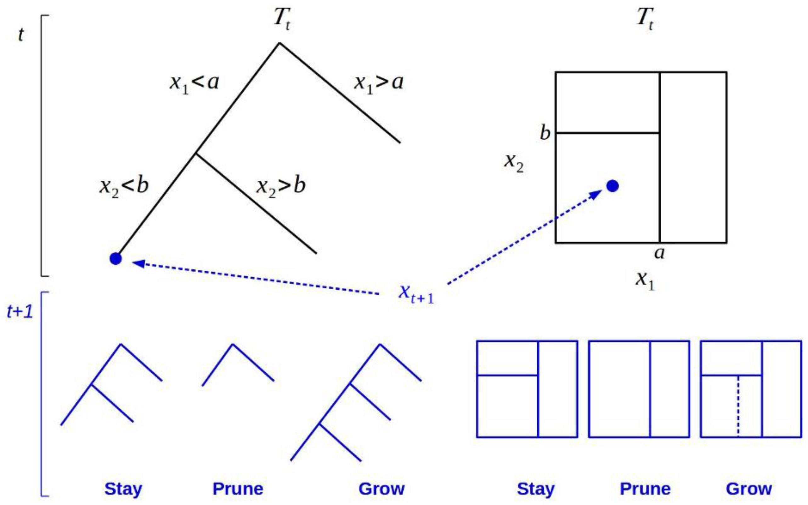
Suppose we have a response variable $\mathit{y}$ and a set of predictor variables $\mathit{x}$. A model for predicting new possible values of $\mathit{y}$ from new values of $\mathit{x}$ will be built by making a partition of the $\mathit{x}$ space into a pool of disjoint sets where the new value of $y$ will have the value associated to theset where the new values of $\mathit{x}$ belong. If we build those disjoint sets by recursively partitioning the data set by one predictor variable at a time then we have a tree $\mathcal{T}$ where the partitions determine a nodes structure. But in an online environment we shall have a time-dependent tree ${\mathcal{T}}_t$ made up of a hierarchy of nodes $\eta \in {\mathcal{T}}_t$ where each of these nodes is related to a disjoint subset of a possibly sequential set of predictor variables ${\mathit{x}}^t={\left\{{\mathit{x}}_s\right\}}_{s=1}^t$ associated to a time-dependent response variable ${\mathit{y}}_t={\left\{y_s\right\}}_{s=1}^t$, where t denotes the time up to which the variables are observed. Figure 1 (top row) illustrates the structure built from the application of recursive split rules on ${\mathit{x}}^t$: it shows how, according to variable constraints, top-down sorting of observations into nodes of a tree is carried out (left plot), and presents the partitioning of the sample space—implied by the split rules—at the bottom of the tree (right plot). The terminal nodes are known as leaves and, for regression trees, they determine a prediction rule for new variable vectors. In this way, any new ${\mathit{x}}_{t+1}$ will be assigned to a single leaf node $\eta \left({\mathit{x}}_{t+1}\right)$, providing a distribution for its prediction ${\mathit{y}}_{t+1}$.

Bayesian trees are determined by a prior distribution and, for obtaining a posterior tree, Bayesian inference makes use of prior and likelihood elements, $p({\mathcal{T}}_t|{\left[\mathit{x},y\right]}^t)\propto p(y_t|{\mathcal{T}}_t,{\mathit{x}}^t)\pi \left({\mathcal{T}}_t\right)$ where the tree prior probability of splitting a node $\eta$ with node depth $D_{\eta }$ is defined by [12] as $p_{split}\left({\mathcal{T}}_t,\eta \right)=\alpha {\left(1+D_{\eta }\right)}^{-\beta }$. If independence across partitions is assumed, the product of likelihoods for each terminal node leads to the availability of a tree likelihood. Given the tree, in order to obtain a conditional model for the leaves, the latter is combined for each leaf node’s parameters with a product of reference or conjugate priors.

DT combine this basic scheme with rules to determine how a given tree is modified when new data arrive. Specifically, for a new tree, the conditional prior $p({\mathcal{T}}_{t+1}|{\mathcal{T}}_t,{\mathit{x}}^{t+1})$ replaces the prior distribution $\mathsf{\pi }\left({\mathcal{T}}_{t+1}\right)$, being the conditional prior restricted to trees obtained from three kind of changes in the neighborhood of the leaf that contains ${\mathit{x}}_{t+1}$, namely: stay and keep the current partitions, prune and get rid of the partition above $\eta \left({\mathit{x}}_{t+1}\right)$, or grow by splitting on the current leaf a new partition. This process introduces stability in the estimation procedure by leveraging the assumed independence structure of trees, that is, our beliefs are changed locally only with regards to the area of the tree around $\eta \left({\mathit{x}}_{t+1}\right)$. Figure 1 also shows the transit from ${\mathcal{T}}_t$ to ${\mathcal{T}}_{t+1}$ through ${\mathit{x}}_{t+1}$.

Although the evolution from ${\mathcal{T}}_t$ to ${\mathcal{T}}_{t+1}$ is thought as a local process when new observations arrive, for inference these strategies must manage the global uncertainty about ${\mathcal{T}}_t$. This is accomplised using a filtering algorithm based on a general particle learning method [29]. Such algorithm uses a finite sample of potential tree particles ${\mathcal{T}}_t^{\left(i\right)}\in \left\{{\mathcal{T}}_t^{\left(1\right)}\dots {\mathcal{T}}_t^{\left(N\right)}\right\}$ containing each the set of tree-defining partition rules to approximate the posterior for ${\mathcal{T}}_t$. The updating of this posterior leads to $\left[{\mathit{x}}_{t+1},y_t\right]$. This is done in two steps. Firstly, a resampling of particles proportional to $p\left(y_t|{\mathcal{T}}_t^{\left(i\right)},{\mathit{x}}_{t+1}\right)$, the predictive probability, is carried out. Secondly, by sampling from $p\left({\mathcal{T}}_{t+1}|{\mathcal{T}}_t^{\left(i\right)},{\left[\mathit{x},y\right]}^{t+1}\right)$ (the conditional posterior), the particles are propagated from the three moves (stay, prune or grow) as depicted in Figure 1. Therefore, although tree propagation is local, global uncertainty is accounted by resampling.

3.1.1. Prediction Rules

In our regression trees the leaves are associated with a prediction rule for any new variable vector. There are two basic prediction rules, both implemented in dynaTree. First of them is the constant mean leaves, where the leaf has a simple response where $\mathbb{E}\left[{\mathrm{y}}_{t+1}|x_{t+1}\right]={\mu }_{\eta \left(x_{t+1}\right)}$, that is, the forecasted value of $y_{t+1}$ will be the mean of the values included in $\eta \left(x_{t+1}\right)$. And the second one, linear leaf, follows a linear rule as ${\mathrm{y}}_{t+1}={\alpha }_{\eta \left(x_{t+1}\right)}+x^t{\beta }_{\eta \left(x_{t+1}\right)}$, that is, the forecasted value of $y_{t+1}$ will be found thanks to the linear model of the values included in $\eta \left(x_{t+1}\right)$.

3.1.2. Retire and Rejuvenate

Although we can keep all the provided data in the DT while the online process is running, we can also retire some $\left[\mathit{x}, y\right]$ pairs. Even if we remove the data the predictive distribution is left unchanged as the information of those retired pairs is in the prior information of the leaves. We shall use two strategies for removing data: the oldest $\left[\mathit{x}, y\right]$ pair, and an active learning algorithm (ACL) [30] which searches for the $\left[\mathit{x}, y\right]$ pair which maximizes the expected reduction in predictive variance averaged over the input space and retires it (for a deeper explanation of its implementation in DT, see [11,31]).

If we choose to retire data, we can optionally choose to create a new particle set with the remaining data, not by deleting the particle set that includes the retired data but by creating a new (rejuvenated) one based only on the remaining active data. The next steps of the online process will determine which of the two particle sets is best for the new distribution.

3.2. Random Forest

Random Forest (RF), first introduced in [8], is also a tree-based method but of a very different nature. It is an ensemble method that fits several trees to a dataset and then combines the predictions of all the trees. The trees grow in an induction procedure by choosing the best split dimension and location from all candidate splits at each node by optimizing a defined criterion (i.e., information gain). But every tree is created not only for a different and randomly subsample of the data set—the strategy known as bagging, where we make resampling with replacement—but for a randomly selected subset of predictors. Once the forest of trees is built, every tree provides a prediction. The value finally predicted for a given observation is calculated as either the most voted class for classification purposes or the average of the predictions for regression problems. In our work, we have used the software for RF available in the randomForest [32] package for R.

Note that RF implies working in a batch mode as all training data are expected to be available in advance and, once a RF is built, it cannot be updated in an incremental way as DT can. For a given new value, we must either always forecast with the previously trained RF or train a whole new RF that includes the old and the new data.

3.3. Experimental Design

As we mentioned before, we shall carry out a first test forecasting one-hour ahead prices to select the best strategies among the wide variety of tested techniques before carrying out a second test forecasting day-ahead prices.

For both tests, all the 2013 data are going to be used as training set and the 2014 data are going to make up the test set, but we must decide the length of the moving window we are going to use for forecasting—that is, the number of previous days we are going to select for predicting the next value. Several studies have investigated the optimum length of the window, for example [15,33] suggest 50 days, being this the length chosen by [9]. Although our study is not about finding the optimal length of the moving window, we are going to try not only with a 50-day length but also with a 10-day length window–the reason to choose the 10 previous days of historical data is that in the literature no studies using windows of short or very-short length exist and this window length will allow us to check, at least in this particular study, whether the short-term effect is decisive in the final price.

In the one-hour ahead test and for DT, we shall test the two basic prediction rules, constant mean and linear. We shall test a full model (keeping all the arriving data without removing any) and a model with removal where we shall test both discarding the oldest data and the data marked by active learning and, for both types of discarding, we shall also test whether to rejuvenate or not the particle set—so at the end we shall have 20 different DT tests. We shall begin to train at the beginning of 2013, we will go through the whole year as in a true online process and only when beginning 2014 we shall start the test process. For RF, and due to its batch nature, we shall train a single model with all the 2013 data and we shall forecast each value of the 2014 year with the same model, but we also want to simulate an online behavior so we shall also train a RF with the last 10 days and another one with the last 50 days, the same rolling window lengths as in DT—note that the “online” RFs for the first days of 2014 will be trained with the last days of 2013. Once we have got results for this one-hour ahead test, we shall choose the best techniques and we shall carry out a second test forecasting day-ahead prices only with the finally selected techniques. As to the execution of DT, we have two parameters ($\alpha ,\beta$) for the tree prior that we could tune to get a result with fewer errors but, following [11], our dynamic trees were fitted using the default parametrization of the dynaTreepackage where the tree prior is specified with $\alpha =0.95$ and $\beta =2$ as inference is generally robust to reasonable changes of these parameters and lead to no significative differences. And regarding the execution of RF, there are several parameters that can be tuned. The number of trees to grow has been set to 200 (the default is 100). The reason to change this parameter is to guarantee more stable results as it is well known from a theoretical point of view that the more trees the more stable the method is [8]. All other parameters have the default values that the randomForest package provides.

3.4. Forecasting Error Evaluation

When, as in our study, we are trying to predict a continuous valued output—the kind of problems known as regression problems—there are two types of statistical metrics used for measuring the forecasting error. First, a measure of the bias of our prediction, which we will define as the arithmetic mean of the errors:

$$\mathrm{BIAS}=\frac{1}{N}{{\displaystyle \sum }}_{i=1}^N({\widehat{y}}_i-y_i),$$

(1)

where ${\widehat{y}}_i$ and $y_i$ are the predicted and the observed values of the variable and $N$ is the length of observed values, and, second, a measure of the accuracy. The two most common measures of accuracy are the Mean Absolute Error (MAE), defined as:

$$\mathrm{MAE}=\frac{1}{N}{{\displaystyle \sum }}_{i=1}^N\left|{\widehat{y}}_i-y_i\right|,$$

(2)

and Root Mean Squared Error (RMSE), defined as:

$$\mathrm{RMSE}=\sqrt{\frac{1}{N}{{\displaystyle \sum }}_{i=1}^N{({\widehat{y}}_i-y_i)}^2}.$$

(3)

Note that, since the errors are squared, the RMSE gives a high weight to very large errors, which means that it is more useful when large errors are undesirable, the kind of errors that could happen in an electricity market so prone to produce spikes (abnormally high prices and also abnormally low prices) as the Iberian market. Also note that these three measures have the same units that the variable to predict so if we want to define relative error measures from these we have to introduce new terms. In our case, we define the same measures but normalized as their original formulations dividing by the mean of the variable to predict ($\overline{y}$) and multiplying by 100, i.e., the Normalized BIAS (NBIAS):

$$\mathrm{NBIAS}=\frac{1}{\overline{y}}\left(\frac{1}{N}{{\displaystyle \sum }}_{i=1}^N{\widehat{y}}_i-y_i\right)\times 100,$$

(4)

the Normalized MAE (NMAE):

$$\mathrm{NMAE}=\frac{1}{\overline{y}}\left(\frac{1}{N}{{\displaystyle \sum }}_{i=1}^N\left|{\widehat{y}}_i-y_i\right|\right)\times 100,$$

(5)

and the Normalized RMSE (NRMSE):

$$\mathrm{NRMSE}=\frac{1}{\overline{y}}\left(\sqrt{\frac{1}{N}{{\displaystyle \sum }}_{i=1}^N{({\widehat{y}}_i-y_i)}^2}\right)\times 100,$$

(6)

which will allow us to establish relative measures against the mean in percent.

But the most widely used measure in the field of EPF is, by far, the Mean Absolute Percentage Error (MAPE), defined as:

$$\mathrm{MAPE}=\frac{1}{N}{{\displaystyle \sum }}_{i=1}^N\left|\frac{{\widehat{y}}_i-y_i}{y_i}\right|,$$

(7)

which is especially useful as it is expressed in percentage terms. Note that MAPE has the disadvantage of being infinite or undefined when $y_i=0$, a value which is relatively usual in our dataset. That’s why we are not going to use it in our study and, instead, we are going to use two variations that try to avoid that problem, the Symmetric MAPE (sMAPE) [34], defined as:

$$\mathrm{sMAPE}=\frac{1}{N}{{\displaystyle \sum }}_{i=1}^{N}2\frac{\left|{\widehat{y}}_i-y_i\right|}{\left|{\widehat{y}}_i\right|+\left|y_i\right|},$$

(8)

and the Mean Arc-tangent Absolute Percentage Error (MAAPE) [35] defined as:

$$\mathrm{MAAPE}=\frac{1}{N}{{\displaystyle \sum }}_{i=1}^{N}ArcTan\left|\frac{{\widehat{y}}_i-y_i}{y_i}\right|.$$

(9)

Note the range of the terms of sMAPE is [0,2], but it cannot avoid completely the problem with $y_i=0$ as it has a maximum value of 2 when either ${\widehat{y}}_i$ or $y_i$ are zero, but is undefined when both are zero, a problem that may appear in our study. Each term of the summation of the MAAPE has a range of [0,$\raisebox{1ex}{$\mathsf{\pi }$}\!\left/ \!\raisebox{-1ex}{$2$}\right.$] and due to the use of the arc-tangent function it can also deal with $y_i=0$ values, but is also undefined when ${\widehat{y}}_i$ and $y_i$ are both zero.

A variation of the MAPE is the Weekly MAPE (WMAPE), defined as:

$$\mathrm{WMAPE}=\frac{1}{N}{{\displaystyle \sum }}_{i=1}^N\frac{\left|{\widehat{y}}_i-y_i\right|}{{\overline{y}}_{week}},$$

(10)

where the denominator is the average weekly price to avoid the adverse effect of prices close or equal to zero; N, the number of hours, here is equal to 168 as it is the number of hours of a whole week (24 h by 7 days).

Note all these measures are not able to give us significant differences in the forecasting performance, that is why we are also going to use the Diebold-Mariano test (DM) [36] for comparing the predictive accuracy of two forecasts. When comparing two forecasts, we shall fix the null hypothesis ($H_0$) as “both methods provide the same forecast accuracy” and our alternative hypothesis ($H_1$) as “the methods have different levels of forecast accuracy”. We have used the DM test version included in the forecast [37] package for R, which incorporates the modified test proposed by Harvey, Leybourne and Newbold [38].

4. Results for the One-Hour Ahead Test

4.1. Dynamic Trees with Constant Mean

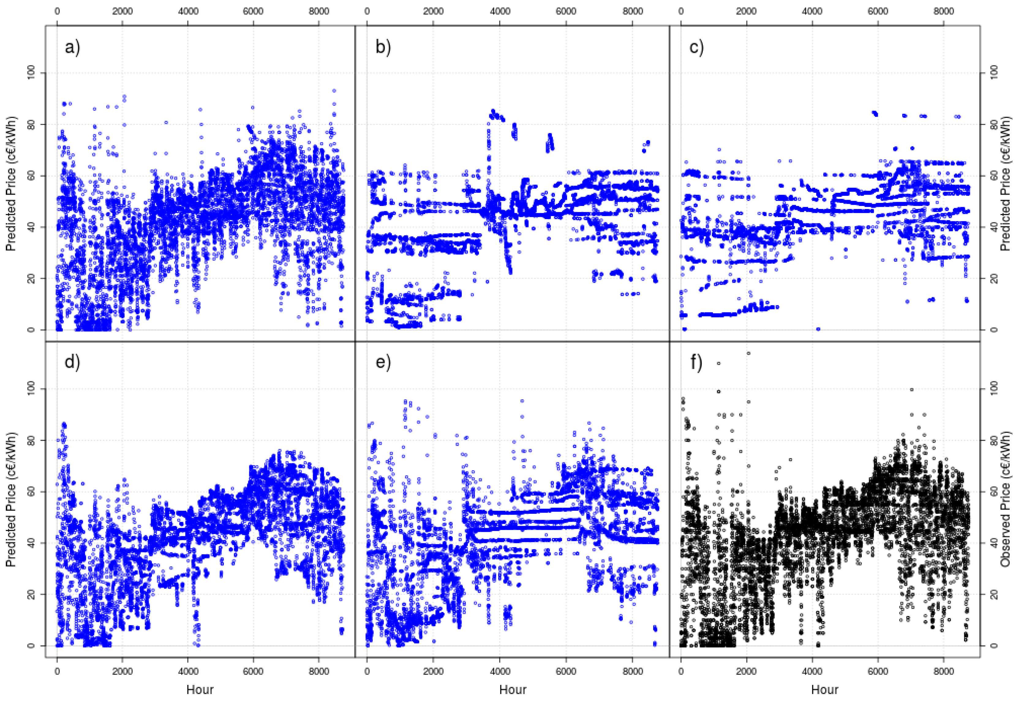
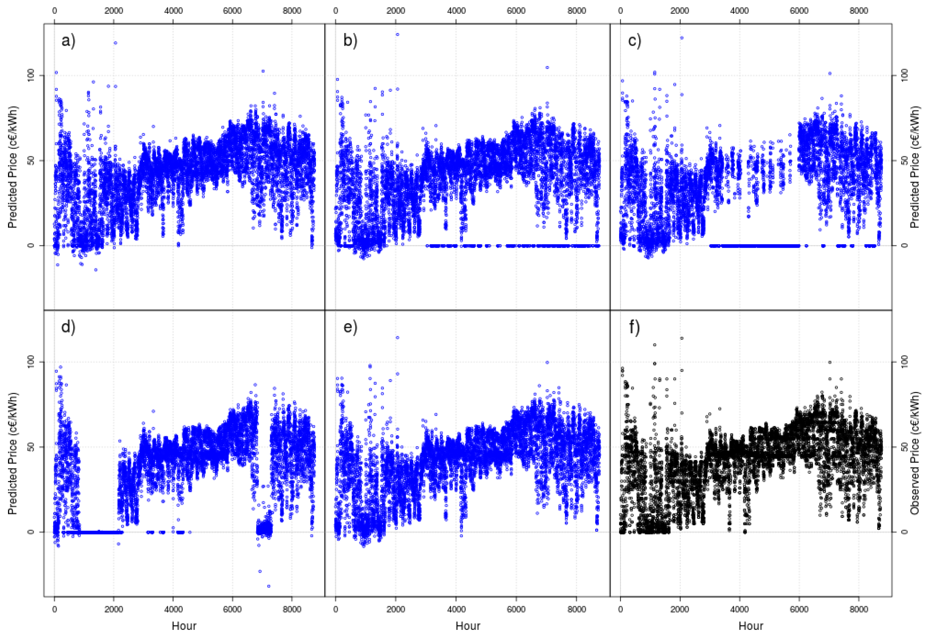
Figure 2 and Figure 3 show the obtained results (in blue points) for DT with constant mean and with rolling windows of 10 (Figure 2) and 50 days (Figure 3) for one-hour ahead forecasting. In order to visually compare the results, we show the observed data as black points (lower right corner in both figures).

Although a visual inspection cannot completely determine the accuracy of a forecast, a naked eye can see a clear effect: except for the full model (where no data are discarded as new data arrive), we can see threads in the plots, especially for models with retirement (both older criteria and active learning criteria) but without rejuvenate, especially for the rolling window of 10 days, and especially for the central part of the image.

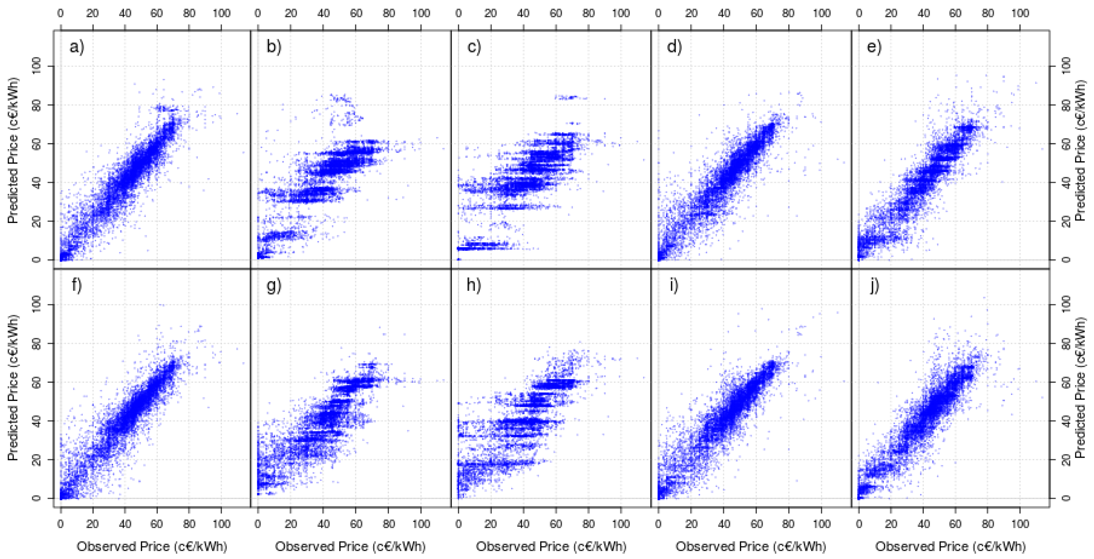
This strange behavior can also be seen in Figure 4, where we have plotted the observed (x) versus the predicted (y) data for both rolling windows (10 days in the upper figures; 50 days in the lower figures). Again, and especially for models with retirement but without rejuvenate (Figure 4b,c,g and h plots) we can see that certain values of predicted data (the horizontal blue lines) are more usual, that is, the models tend to forecast a few particular values instead of performing, for instance, as the full model (Figure 4a and f), which provides different outputs for different inputs.

Table 2. Tree statistics for the different used types of DT with constant mean, for rolling windows of 10 and 50 days.

Window Length	Model Type	Average Tree Height	Average Number of Leaves	Average Leaf Size
10	Full	23	1235.106	14.18607
	Retire Oldest	12.061	86.824	2.767684
	Retire ACL	12	74.961	3.203759
	Retire Oldest & Rejuvenate	10.562	28.245	8.55525
	Retire ACL & Rejuvenate	9.254	42.94	6.209573
50	Full	23	1274.049	13.75236
	Retire Oldest	14.017	114.152	10.51965
	Retire ACL	17.549	143.476	8.365751
	Retire Oldest & Rejuvenate	11.949	119.387	10.0582
	Retire ACL & Rejuvenate	13	136.238	8.817967

provides an explanation for this behavior. In this table we show statistics of the height, number of leaves and leaf size for the trees created for every different used type of DT. As we can see, the average of these measures has a high value for the full model and a small value for the other ones. That is, when new data arrive the full model can predict a new value associated to a great variety of leaves and therefore this full model can provide a great variety of outputs. However, the other models have a small number of leaves for the generation of a new prediction and as a consequence these models will tend to provide always the same outputs from the same limited set of leaves. Note that the tree statistics for the models with rejuvenate are similar to the models without it, but their behavior is different, showing that for our EPF problem the rejuvenate process avoids the problem of always providing the same small set of output values.

Table 3. One-hour ahead forecasting error evaluation for the different used types of DT with constant mean, for rolling windows of 10 and 50 days. BIAS, Root Mean Squared Error (RMSE) and Mean Absolute Error (MAE) are in the same units as the electricity price (c€/kWh); Normalized BIAS (NBIAS), Normalized RMSE (NRMSE), Normalized MAE (NMAE), Symmetric MAPE (sMAPE) and Mean Arc-tangent Absolute Percentage Error (MAAPE) are in percentage.

Window Length	Model Type	BIAS	NBIAS	RMSE	NRMSE	MAE	NMAE	sMAPE	MAAPE
10	Full	0.31	0.75	6.56	15.85	4.44	10.71	0.21	0.19
	Retire Oldest	0.24	0.57	10.16	24.56	7.2	17.41	0.26	0.25
	Retire ACL	−0.06	−0.15	10.55	25.49	7.76	18.76	0.29	0.27
	Retire Oldest & Rejuvenate	0.39	0.95	7.25	17.53	4.66	11.25	0.21	0.19
	Retire ACL & Rejuvenate	0.18	0.43	6.55	15.82	4.62	11.15	0.22	0.2
50	Full	−0.17	−0.41	6.84	16.53	4.52	10.93	0.22	0.19
	Retire Oldest	−0.8	−1.93	9.22	22.28	6.6	15.94	0.27	0.25
	Retire ACL	0.09	0.22	10.55	25.48	7.65	18.48	0.29	0.27
	Retire Oldest & Rejuvenate	0.39	0.94	7.16	17.31	4.79	11.58	0.22	0.2
	Retire ACL & Rejuvenate	0.18	0.44	6.85	16.56	4.73	11.44	0.21	0.19

shows the forecasting error evaluation for every different used type of DT with constant mean. As expected, all the statistics for the retire-without-rejuvenate models are the worst ones, so this kind of models will not be considered in our next comparisons. Although similar for most statistics, BIAS and RMSE (and their normalized versions) show that before rejuvenate, to retire with the active learning criteria is better than to retire the oldest data, that is, retiring the oldest data tend to provide large errors, an effect we want to avoid when forecasting the electricity price. That is why, from the DT with constant mean test, we will finally choose the full model and then retire with active learning criteria plus a rejuvenate model for future comparisons.

4.2. Dynamic Trees with Linear Model

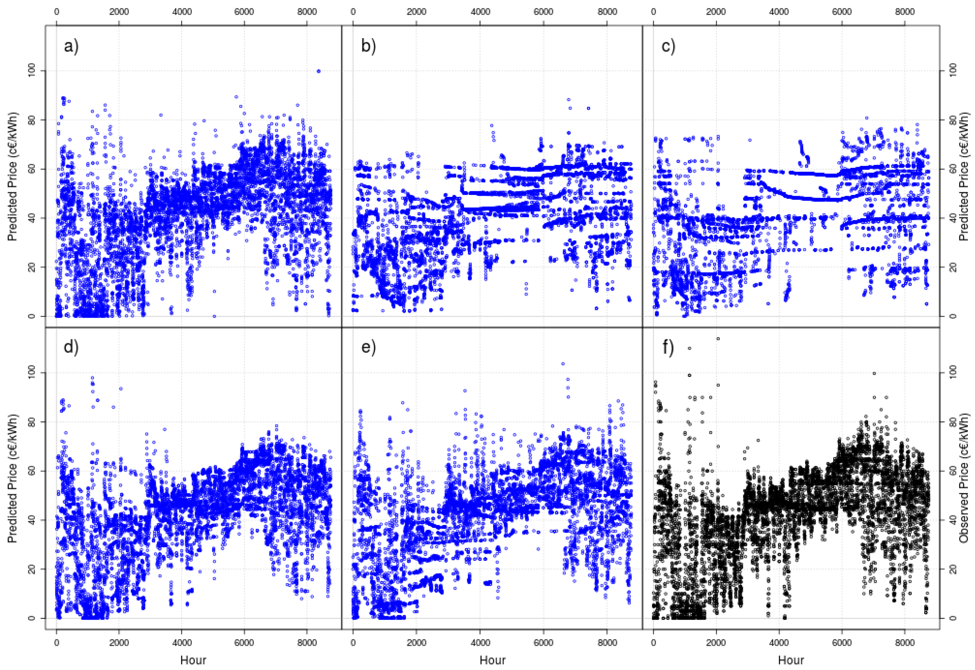
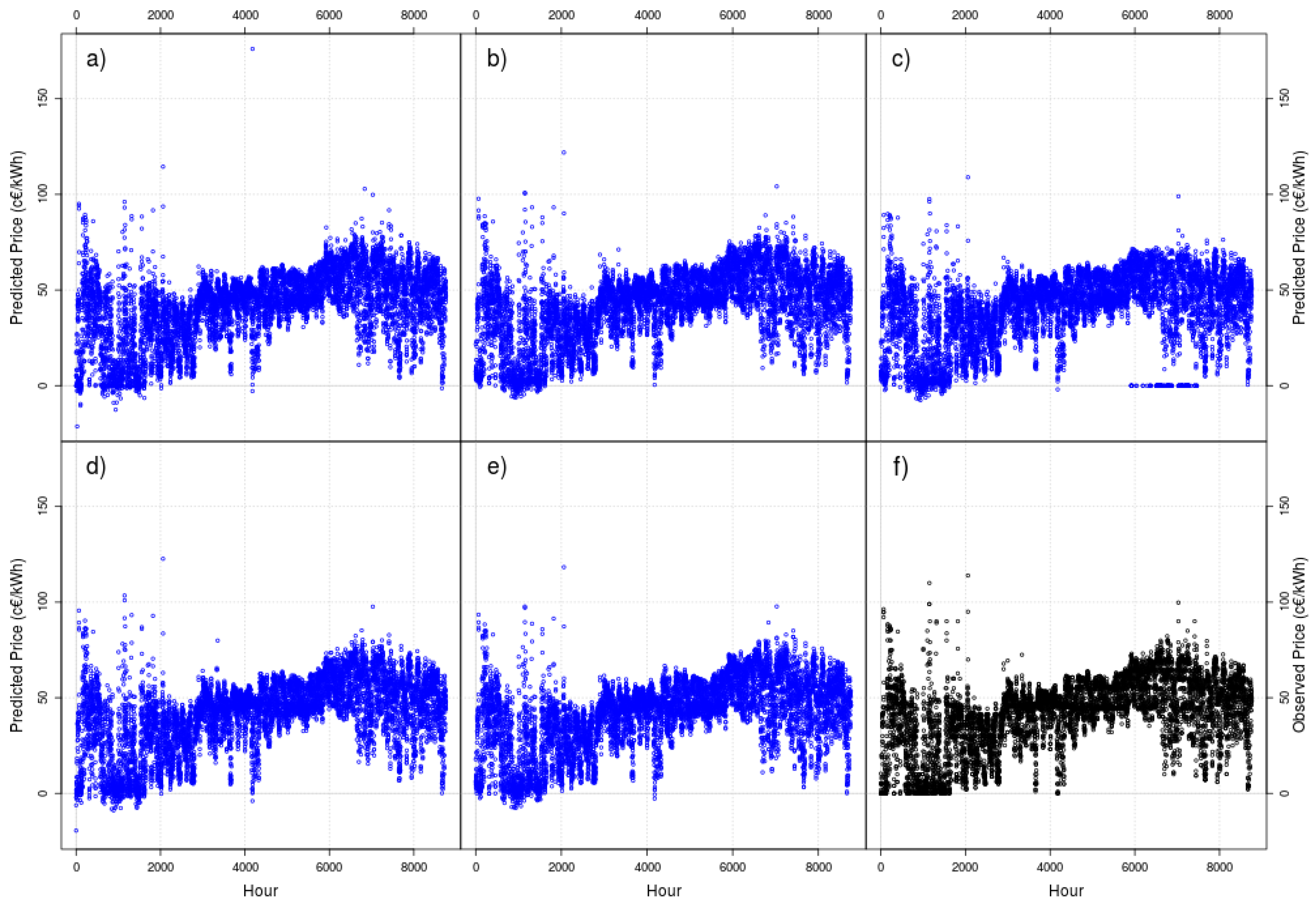
Figure 5 and Figure 6 show the one-hour ahead forecast results (as blue points) for DT with linear model and a rolling windows of 10 (Figure 5) and 50 days (Figure 6)—again, to visually compare the results, we show the observed data as black points (lower right corner in both figures).

A visual inspection of the figures does not show any phenomena as strange as the threads shown in the case of DT with constant mean, but there are two striking results: the negative values and the abundance of zeros (especially in the model with a window length of 10 days). There are no negative prices in the Iberian market—these negative values can be explained due to the fact that any linear model can predict negative values, and that is the effect that new data (for t + 1) can produce in old linear models (built with data included at least from 0 to t).

Table 4. One-hour ahead forecasting error evaluation for the different used types of DT with linear model, for rolling windows of 10 and 50 days. BIAS, RMSE and MAE are in the same units as the electricity price (c€/kWh); NBIAS, NRMSE, NMAE, sMAPE and MAAPE are in percentage.

Window Length	Model Type	BIAS	NBIAS	RMSE	NRMSE	MAE	NMAE	sMAPE	MAAPE
10	Full	−0.01	−0.02	4.03	9.73	2.53	6.11	NaN	NaN
	Retire Oldest	−4.94	−11.93	16.89	40.8	7.47	18.05	0.34	0.21
	Retire ACL	−13.77	−33.27	26.43	63.84	15.65	37.81	NaN	NaN
	Retire Oldest & Rejuvenate	−6.81	−16.46	17.75	42.89	8.68	20.97	NaN	NaN
	Retire ACL & Rejuvenate	−0.21	−0.51	4.1	9.92	2.76	6.66	0.16	0.14
50	Full	0.08	0.18	4.3	10.4	2.48	5.98	NaN	NaN
	Retire Oldest	−0.04	−0.09	4.16	10.04	2.79	6.74	0.15	0.14
	Retire ACL	−1.67	−4.04	11.55	27.91	4.34	10.49	0.2	0.16
	Retire Oldest & Rejuvenate	−0.17	−0.4	4.38	10.58	2.64	6.38	0.16	0.14
	Retire ACL & Rejuvenate	−0.13	−0.31	3.98	9.61	2.66	6.42	0.15	0.14

shows the forecasting error evaluation for every different used type of DT with linear model. Note that due to the high number of times that ${\widehat{y}}_i=0,$ and as there are times where $y_i=0$, sMAPE and MAAPE may be undefined (NaN). Also note that, due to the existence of predicted negative prices, and except for a single model type, BIAS is negative. In the case of a window length of 10 days, it is clear that the best two models are the full model and the retire with active learning criteria plus rejuvenate model. We will use these two models in our next comparisons. In the case of a window length of 50 days, and except in the model with retiring by active learning (the worst), the differences between models are much smaller—especially if our criteria are sMAPE and MAAPE (when available).

As we want to select another model, our final decision is to choose the full model (the best in terms of MAE), that is, DT with no extra treatment of the included data (full model: no retirement and no rejuvenation) and a model with (in this case, the retire with active learning criteria plus rejuvenate model).

4.3. Batch and “Online” Random Forest

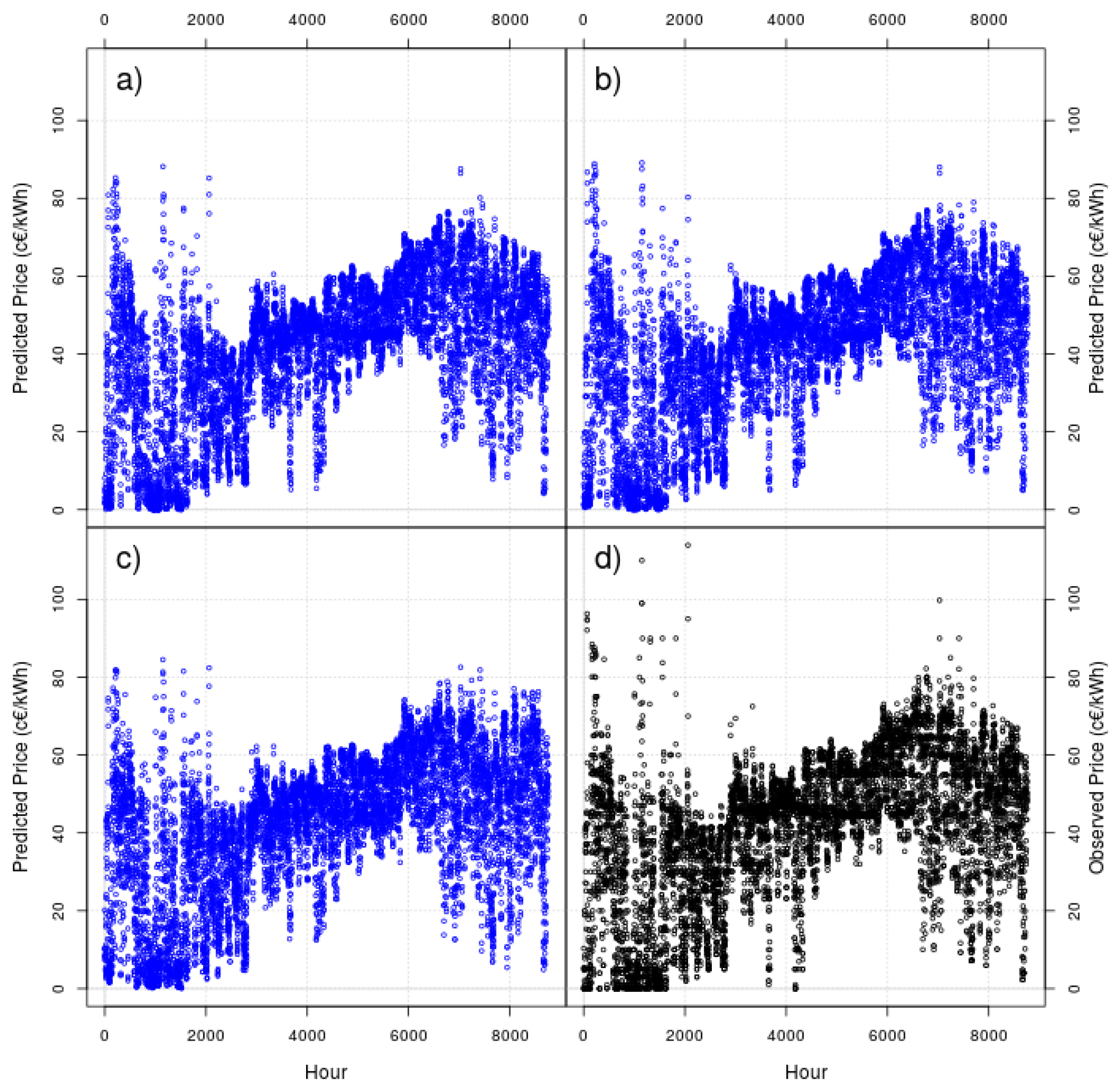
Figure 7 shows the one-hour ahead results (as blue points) for RF, for an “online” RF with rolling windows of 10 and 50 days and for a RF running in batch mode—again, to visually compare the results, we show the observed data as black points (lower right corner).

A visual inspection of the figure does not show any strange phenomena, as it could be expected for a method as reliable like random forest. For a naked eye, the three tested RF provide accurate results very similar to the observed data.

Table 5. One-hour ahead forecasting error evaluation for the different used types of RF. BIAS, RMSE and MAE are in the same units as the electricity price (c€/kWh); NBIAS, NRMSE, NMAE, sMAPE and MAAPE are in percentage.

Model Type	BIAS	NBIAS	RMSE	NRMSE	MAE	NMAE	sMAPE	MAAPE
Batch	0.77	1.86	4.33	10.46	2.99	7.23	0.16	0.15
“Online” 10	0.07	0.17	4.77	11.52	3.09	7.46	0.16	0.15
“Online” 50	0.12	0.28	4.12	9.96	2.64	6.37	0.15	0.14

shows the forecasting error evaluation for every different type of RF. It can be observed that the “online” RF with a window length of 50 days is clearly the best model. But, and although it is not strictly necessary, as it is its “pure” form, we are also going to keep the batch RF for our next comparisons (although it is worse than the “online” version with a window length of 50 days).

4.4. Performance Comparison

For the sake of clarity, and because of the many DT employed variations, the following table (

Table 6. Acronyms of the final DT methods to be compared.

Prediction Rule	Window Length	Model	Plus	Acronym
Constant Mean	10	Full Model	-	DT.Mean.10.Full
		Retirement with active learning	-	DT.Mean.10.RAcl
		Retirement with active learning	Rejuvenate	DT.Mean.10.RAcl.Rej
	50	Full Model	-	DT.Mean.50.Full
		Retirement with active learning	-	DT.Mean.50.RAcl
		Retirement with active learning	Rejuvenate	DT.Mean.50.RAcl.Rej
Linear Model	10	Full Model	-	DT.Lin.10.Full
		Retirement with active learning	-	DT.Lin.10.RAcl
		Retirement with active learning	Rejuvenate	DT.Lin.10.RAcl.Rej
	50	Full Model	-	DT.Lin.50.Full
		Retirement with active learning	-	DT.Lin.50.RAcl
		Retirement with active learning	Rejuvenate	DT.Lin.50.RAcl.Rej

) summarizes the final DT methods to be compared and their acronyms:

Table 7. One-hour ahead forecasting error evaluation for the different models used in our final comparison. BIAS, RMSE and MAE are in the same units as the electricity price (c€/kWh); NBIAS, NRMSE, NMAE, sMAPE and MAAPE are in percentage.

Model	Model Type	BIAS	NBIAS	RMSE	NRMSE	MAE	NMAE	sMAPE	MAAPE
DT mean 10	Full	0.31	0.75	6.56	15.85	4.44	10.71	0.21	0.19
	Retire ACL & Rejuvenate	0.18	0.43	6.55	15.82	4.62	11.15	0.22	0.2
DT mean 50	Full	−0.17	-0.41	6.84	16.53	4.52	10.93	0.22	0.19
	Retire ACL & Rejuvenate	0.18	0.44	6.85	16.56	4.73	11.44	0.21	0.19
DT linear 10	Full	−0.01	−0.02	4.03	9.73	2.53	6.11	NaN	NaN
	Retire ACL & Rejuvenate	−0.21	−0.51	4.1	9.92	2.76	6.66	0.16	0.14
DT linear 50	Full	0.08	0.18	4.3	10.4	2.48	5.98	NaN	NaN
	Retire ACL & Rejuvenate	−0.13	−0.31	3.98	9.61	2.66	6.42	0.15	0.14
RF	Batch	0.77	1.86	4.33	10.46	2.99	7.23	0.16	0.15
	“Online” 50	0.12	0.28	4.12	9.96	2.64	6.37	0.15	0.14

shows the one-hour ahead forecasting error evaluation for the final models to be compared; it shows the same information that appears in Table 3, Table 4 and Table 5 but only for the selected models, in order to be compared in a single table. We have written in bold the best result for every statistic (when available).

Although sMAPE and MAAPE cannot give us significant enough information to determine the best model, but for the fact that they mark DT with constant mean as the worst method (both with a window length of 10 or 50 days), RMSE and MAE (and their normalized versions) can do. According to the RMSE, DT.Lin.50.RAcl.Rej is the best model, followed by DT.Lin.10.Full and DT.Lin.10.RAcl.Rej, the latter similar to the “online” RF with a window length of 50 days. According to the MAE, DT.Lin.50.Full is the best one, followed by DT.Lin.10.Full and the “online” RF with a window length of 50 days, the latter similar to the DT.Lin.50.RAcl.Rej. Note that both RMSE and MAE also mark DT with constant mean as the worst method. According to the BIAS (with regards to its magnitude and not its sign), DT.Lin.10.Full is the best model, followed by DT.Lin.50.Full and the “online” RF with a window length of 50 days, the latter similar to DT.Lin.50.RAcl.Rej.

All of the above show that DT with linear model and a window length of 50 days achieves better results than RF (no matter if it is an “online” or a batch running) for our EPF problem. Depending on the criteria used, we could choose either a model with retirement with active learning criteria plus rejuvenate (if we choose the RMSE) or a full model (if we choose the MAE). Given the squared terms in the RMSE closed formula, more importance is given to larger errors, so we think that RMSE is an appropriate measure as we want to penalize large errors in EPF since they could produce large monetary losses in a real market environment. So, our final choice would be DT.Lin.50.RAcl.Rej.

Unfortunately, the results shown in Table 7 do not give us significant differences, as we only have one test—the whole year 2014 in an online process. That’s why we are going to use the DM test for comparing the final models. We are going to use DM several times, comparing the models to each other through a series of steps discarding the ones with less accuracy and looking for the comparisons among the best models with the aim of finding the best model.

Table 8. One-hour ahead forecast results for the Diebold-Mariano test.

Model 1	Model 2	${\mathit{H}}_0$	${\mathit{H}}_1$	p-Value
DT mean 10: Full	DT Mean 10: Retire ACL & Rejuvenate	${\mathit{Accuracy}}_{\mathbf{1}}={\mathit{Accuracy}}_{\mathbf{2}}$	$Accurac{y}_1\ne Accurac{y}_2$	0.9039
		$Accurac{y}_1=Accurac{y}_2$	$Accurac{y}_1<Accurac{y}_2$	0.4519
		$Accurac{y}_1=Accurac{y}_2$	$Accurac{y}_1>Accurac{y}_2$	0.5481
DT mean 50: Full	DT Mean 50: Retire ACL & Rejuvenate	${\mathit{Accuracy}}_{\mathbf{1}}={\mathit{Accuracy}}_{\mathbf{2}}$	$Accurac{y}_1\ne Accurac{y}_2$	0.9358
		$Accurac{y}_1=Accurac{y}_2$	$Accurac{y}_1<Accurac{y}_2$	0.5321
		$Accurac{y}_1=Accurac{y}_2$	$Accurac{y}_1>Accurac{y}_2$	0.4679
DT linear10: Full	DT Linear 10: Retire ACL & Rejuvenate	${\mathit{Accuracy}}_{\mathbf{1}}={\mathit{Accuracy}}_{\mathbf{2}}$	$Accurac{y}_1\ne Accurac{y}_2$	0.2928
		$Accurac{y}_1=Accurac{y}_2$	$Accurac{y}_1<Accurac{y}_2$	0.8536
		$Accurac{y}_1=Accurac{y}_2$	$Accurac{y}_1>Accurac{y}_2$	0.1464
DT linear 50: Full	DT Linear 50: Retire ACL & Rejuvenate	${\mathit{Accuracy}}_{\mathbf{1}}={\mathit{Accuracy}}_{\mathbf{2}}$	$Accurac{y}_1\ne Accurac{y}_2$	0.45
		$Accurac{y}_1=Accurac{y}_2$	$Accurac{y}_1<Accurac{y}_2$	0.225
		$Accurac{y}_1=Accurac{y}_2$	$Accurac{y}_1>Accurac{y}_2$	0.775
RF “Online” 50	RF Batch	$Accurac{y}_1=Accurac{y}_2$	$Accurac{y}_1\ne Accurac{y}_2$	5.494×10−7
		$Accurac{y}_1=Accurac{y}_2$	$Accurac{y}_1<Accurac{y}_2$	1
		$Accurac{y}_1=Accurac{y}_2$	${\mathit{Accuracy}}_{\mathbf{1}}>{\mathit{Accuracy}}_{\mathbf{2}}$	2.747×10−7
DT Mean 10: Retire ACL & Rejuvenate	DT Mean 50: Full	$Accurac{y}_1=Accurac{y}_2$	$Accurac{y}_1\ne Accurac{y}_2$	0.007294
		$Accurac{y}_1=Accurac{y}_2$	$Accurac{y}_1<Accurac{y}_2$	0.9964
		$Accurac{y}_1=Accurac{y}_2$	${\mathit{Accuracy}}_{\mathbf{1}}>{\mathit{Accuracy}}_{\mathbf{2}}$	0.003647
DT Linear10: Full	DT Linear 50: Retire ACL & Rejuvenate	${\mathit{Accuracy}}_{\mathbf{1}}={\mathit{Accuracy}}_{\mathbf{2}}$	$Accurac{y}_1\ne Accurac{y}_2$	0.5308
		$Accurac{y}_1=Accurac{y}_2$	$Accurac{y}_1<Accurac{y}_2$	0.2654
		$Accurac{y}_1=Accurac{y}_2$	$Accurac{y}_1>Accurac{y}_2$	0.7346
DT Mean 10: Retire ACL & Rejuvenate	DT Linear 50: Retire ACL & Rejuvenate	$Accurac{y}_1=Accurac{y}_2$	$Accurac{y}_1\ne Accurac{y}_2$	< 2×10−16
		$Accurac{y}_1=Accurac{y}_2$	${\mathit{Accuracy}}_{\mathbf{1}}<{\mathit{Accuracy}}_{\mathbf{2}}$	< 2×10−16
		$Accurac{y}_1=Accurac{y}_2$	$Accurac{y}_1>Accurac{y}_2$	1
RF “Online” 50	DT Linear 50: Retire ACL & Rejuvenate	$Accurac{y}_1=Accurac{y}_2$	$Accurac{y}_1\ne Accurac{y}_2$	0.001018
		$Accurac{y}_1=Accurac{y}_2$	${\mathit{Accuracy}}_{\mathbf{1}}<{\mathit{Accuracy}}_{\mathbf{2}}$	0.0005092
		$Accurac{y}_1=Accurac{y}_2$	$Accurac{y}_1>Accurac{y}_2$	0.9995

shows the results of our battery of DM tests—we have written in bold the final winning hypothesis and its p-value.

In the first five tests we have compared model pairs that follow the same strategy. The results show that:

(1)

Regarding the DT.Mean.10 strategy, no matter which model we choose, they have similar accuracy (we cannot reject the null hypothesis $H_0$ “both methods provide the same forecast accuracy”) as none of the p-values of the tests of equal accuracies are smaller than 0.05 (our level of significance). As the p-value shows a slightly preference for DT.Mean.10.RAcl.Rej, we choose this one for the next round.

(2)

Concerning the DT.Mean.50 strategy, no matter which model we choose, they have similar accuracy (we cannot reject the null hypothesis). As the p-value shows a slightly preference for DT.Mean.50.Full, we choose this one for the next round.

(3)

With regards to the DT.Lin10 strategy, no matter which model we choose, they have similar accuracy (we cannot reject the null hypothesis). We choose DT.Lin.10.Full as the best one as the p-value shows a slightly preference for that hypothesis.

(4)

Regarding the DT.Lin.50 strategy, and although none of the p-values of the tests of equal accuracies are smaller than 0.05 and so we can conclude that they have similar accuracy (we cannot reject the null hypothesis), we choose DT.Lin.50.RAcl.Rej as the best one as the p-value shows a slightly preference for that hypothesis.

(5)

Concerning the RF strategy, the “online” RF with a window length of 50 days is clearly more accurate than the batch RF.

Now that we have chosen the best models, let us compare them. The next four tests in Table 8 show that:

(6)

In the comparison between the DT.Mean.10strategy and the DT.Mean.50 strategy, it is clearly better the DT.Mean.10 strategy. In our case, DT.Mean.10.RAcl.Rej although we must remember that it was almost indistinguishable of the full model.

(7)

In the comparison between the DT.Lin.10 strategy and the DT.Lin.50 strategy, and although none of the p-values of the tests of equal accuracies are smaller than 0.05 (and therefore we cannot reject the null hypothesis), we choose the model of 50 days (DT.Lin.50.RAcl.Rej) as the best one given that the p-value shows a slightly preference for that hypothesis.

(8)

In the comparison between the DT.Mean.10 strategy and the DT.Lin.50 strategy (specifically, DT.Mean.10.RAcl.Rejand DT.Lin.50.RAcl.Rej), the test clearly shows that DT.Lin.50 is more accurate (specifically, DT.Lin.50.RAcl.Rej).

(9)

In the comparison between the “online” RF strategy with a window length of 50 days and DT.Lin.50 (specifically, DT.Lin.50.RAcl.Rej), the test clearly shows that DT.Lin.50 is more accurate (specifically, DT.Lin.50.RAcl.Rej).

Note that the result is completely coherent with the one obtained in our forecasting error evaluation previously shown in Table 7: DT.Lin.50.RAcl.Rej is the best model for our EPF one-hour ahead problem test.

5. Results for the One-Day Ahead Test

Although Section 4 showed us that DT.Lin.50.RAcl.Rej is the best model for the one-hour ahead test, it also showed that, from a wider point of view, the DT.Lineal strategy is the best one. That is why, for the one-day ahead test, we are going to use the whole DT.Lin.50 strategy, that is, its five variations and not only its DT.Lin.50.RAcl.Rej specific variation. And following our previous tests, we are also going to use the best RF version, that is, the RF “Online” with a rolling window of 50 days to complete our test.

Table 9. One-day ahead forecasting error evaluation for the different selected types of DT with linear model and for the selected “Online” RF, for a rolling window of 50 days. BIAS, RMSE and MAE are in the same units as the electricity price (c€/kWh); NBIAS, NRMSE, NMAE, sMAPE and MAAPE are in percentage.

Model	Model Type	BIAS	NBIAS	RMSE	NRMSE	MAE	NMAE	sMAPE	MAAPE
DT	Full	0.08	−0.20	3.49	8.42	2.24	5.40	NaN	NaN
	Retire Oldest	−3.16	−4.62	12.89	31.07	5.29	12.76	NaN	NaN
	Retire ACL	−1.67	−4.04	7.36	17.74	4.11	9.91	NaN	NaN
	Retire Oldest & Rejuvenate	0.01	0.02	3.75	9.05	2.48	5.97	NaN	NaN
	Retire ACL & Rejuvenate	−0.01	−0.03	3.88	9.35	2.61	6.30	NaN	NaN
RF	“Online”	0.33	0.80	4.48	10.79	2.96	7.13	0.16	0.15

shows the one-day ahead forecasting error evaluation for the final models. We have written in bold the best result for every statistic (when available).

With regard to the DT models the ones with retirement but without rejuvenate are clearly the worst ones. The other versions (full model and models with rejuvenate) perform in a very similar manner, although in this comparison DT.Lin.50.RAcl.Rej is not the best one, being outperformed in the RMSE (and also in the MAE) by the method with retire of the oldest data and specially by the full model—as expected, the “Online” RF method is outperformed by the three best DT lineal models (the full one and the versions with rejuvenate).

Again, as in Section 4, we are going to use the DM test for the comparison of the final models through a series of steps discarding the ones with less accuracy and looking for the comparisons among the best models.

Table 10. One-Day ahead forecast results for the Diebold-Mariano test.

Model 1	Model 2	${\mathit{H}}_0$	${\mathit{H}}_1$	p-Value
DT Lineal50: Retire Oldest& Rejuvenate	DT Lineal50: Retire ACL & Rejuvenate	$Accurac{y}_1=Accurac{y}_2$	$Accurac{y}_1\ne Accurac{y}_2$	0.0051
		$Accurac{y}_1=Accurac{y}_2$	$Accurac{y}_1<Accurac{y}_2$	0.9974
		$Accurac{y}_1=Accurac{y}_2$	${\mathit{Accuracy}}_{\mathbf{1}}>{\mathit{Accuracy}}_{\mathbf{2}}$	0.0025
DT Lineal 50: Full	DT Lineal 50: Retire Oldest& Rejuvenate	$Accurac{y}_1=Accurac{y}_2$	$Accurac{y}_1\ne Accurac{y}_2$	3.74×10−5
		$Accurac{y}_1=Accurac{y}_2$	$Accurac{y}_1<Accurac{y}_2$	1
		$Accurac{y}_1=Accurac{y}_2$	${\mathit{Accuracy}}_{\mathbf{1}}>{\mathit{Accuracy}}_{\mathbf{2}}$	1.87×10−5
DT Lineal 50: Full	RF “Online” 50	$Accurac{y}_1=Accurac{y}_2$	$Accurac{y}_1\ne Accurac{y}_2$	2.2×10−16
		$Accurac{y}_1=Accurac{y}_2$	$Accurac{y}_1<Accurac{y}_2$	1
		$Accurac{y}_1=Accurac{y}_2$	${\mathit{Accuracy}}_{\mathbf{1}}>{\mathit{Accuracy}}_{\mathbf{2}}$	2.2×10−16

shows the results of our battery of DM tests—we have written in bold the finally winning hypothesis and its p-value.

The results of the DM tests show that:

(1)

In the comparison between the two DT.Lin.50 strategies with retirement and rejuvenate, the test clearly shows that DT.Lin.50 with retirement of the oldest data is more accurate.

(2)

In the comparison between the DT.Lin.50.Fullstrategy and the DT.Lin.50 with retirement of the oldest data and rejuvenate strategy, the test clearly shows that DT.Lin.50.Fullis more accurate.

(3)

In the comparison between the “online” RF strategy with a window length of 50 days and DT.Lin.50.Full, the test clearly shows that DT.Lin.50.Full is more accurate.

This result is completely coherent with the one obtained in our forecasting error evaluation (previously shown in Table 9): DT.Lin.50.Full is the best model for our EPF one-day ahead problem test.

Comparison with Previous Studies on the Iberian Market

Up to now we have been studying how to use the DT technique to face the EPF problem, by using the available data and benchmarking against another tree-based technique, RF. Now we want to compare our results for DT against the results obtained by other researchers in other studies using other techniques. Unfortunately, there are no sets of tests for year 2014, the year for which we have conducted our previous tests, but, thanks to some original works [15,37] we have at our disposal several forecasting results for the year 2002. In those works, as representatives of the four seasons of the year, the fourth week of February (Winter), May (Spring), August (Summer), and September (Fall) are selected, i.e., weeks with a particularly good price performance are not sought after on purpose. These full (from Monday to Sunday) selected weeks are 18–24 February, 20–26 May,19–25 August and 18–24 November of the year 2002. For our study, and also looking for the similar four full weeks, we have chosen 17–23 February, 19–25 May, 18–24 August and 17–23 November of year 2014, in order to compare the results for the four seasons of the year.

This may not seem a fair comparison. First of all, the forecasted years are not the same ones and the results cannot be strictly compared, and in all these years (from 2002 to 2014) the conditions of the Iberian market have changed dramatically (for example, with the increasing role of the renewable energies). However, it is important to remark that this is not a quantitative comparison but a qualitative one, to find out if the results of the DT forecast makes sense.

Table 11. Weekly MAPE (WMAPE) (%) for the four representative weeks of the four seasons of the year for several studies. As the results of our work (in italic) are for the year 2014 and the other studies are for the year 2002, these statistics must be treated with great care and so interpreted only in a qualitative way.

Reference	Technique	Winter	Spring	Summer	Fall	Average
	Dynamic Trees	13.45	5.63	2.95	4.86	7.56
[15]	Naïve	7.68	7.27	27.30	19.98	15.58
[39]	ARIMA	6.32	6.36	13.39	13.78	9.96
[15]	Wavelet-ARIMA	4.78	5.69	10.70	11.27	8.11
[40]	Neural Network	5.23	5.36	11.40	13.65	8.9
[41]	Weighted Nearest Neighbors	5.15	4.34	10.89	11.83	8.05
[20]	Fuzzy Neural Network	4.62	5.30	9.84	10.32	7.52
[42]	Pattern Sequence Similarity	5.98	4.51	9.11	10.07	7.42
[43]	Wavelets & Fuzzy Neural Network	3.38	4.01	9.47	9.27	6.53
[31]	Mutual Information & Neural Network & Evolutionary Algorithm	4.88	4.65	5.79	5.96	5.32
[44]	SOM Cluster Pattern Sequence-based NextSymbolPrediction	3.96	3.59	5.32	6.18	4.76

shows the WMAPE (in %) for the four representative weeks of the four seasons of the year for our best DT study (in the first line in italic), DT.Lin.50.Full, and several studies, sorted by the seasonal average. As it can be observed, the seasonal average of our DT study has the same magnitude of the rest of the studies, which seems to indicate that DT is a reliable technique for the EPF problem—note that although the testing years are not the same, we can conclude that this DT method is comparable to the others and could be used in a real forecasting environment.

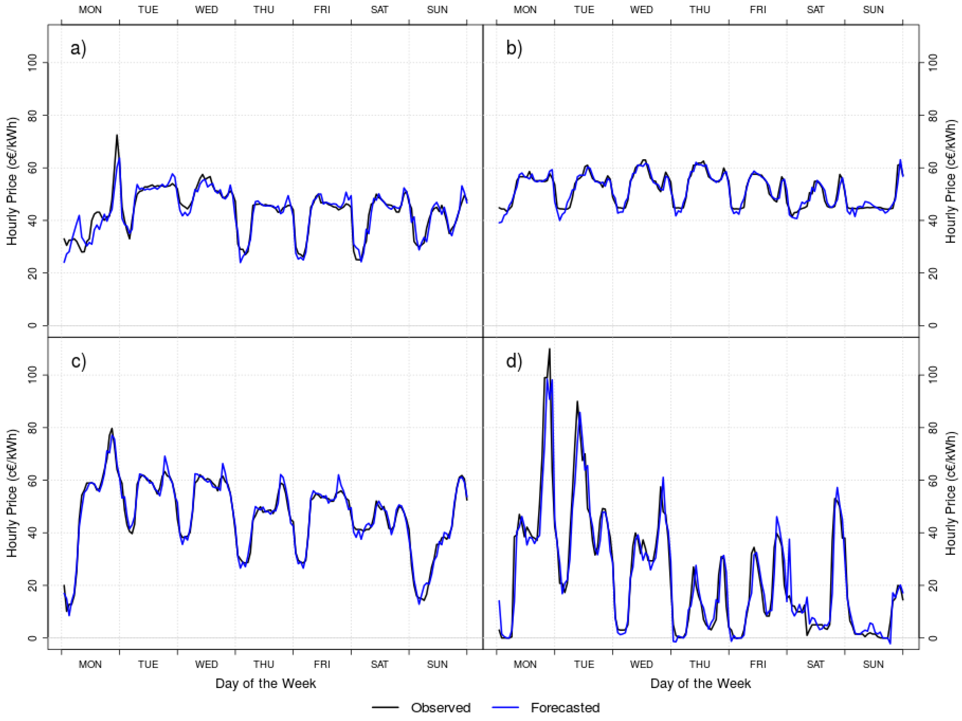
As observed in Table 11, the seasonal results for DT.Lin.50.Full show a very different behavior to the rest of the studies, as Summer and Fall have a lower WMAPE, and Winter provides the highest WMAPE, while in the remaining studies Summer and Fall use to reach the highest WMAPE and Winter usually attains a low WMAPE. In Figure 8 we have plotted the observed (black lines) and the forecasted (blue lines) hourly prices for the four representative weeks of the four seasons.

As expected, Summer (b) and Fall (c) show how close of the observed data are the DT forecasts of DT.Lin.50.Full. However for Winter (d), the strong variability of the prices and the high spikes produce a great difficulty of forecast leading the most misguided season. Up to our experience, there is a reason for this difficulty, not only for year 2014 but also nowadays: in Spain, due to the strong wind variability in February and to the influence of the wind energy in the final energy prices, this month’s forecast is usually the most difficult to predict. Further studies with more recent data should face this situation (which was not happening in 2002), and establish new comparisons among different techniques.

6. Conclusions

Because of its importance to society and for energy operators and investors, Electricity Price Forecasting is a complex problem that has been studied over time using different methodologies. Machine learning is one of those general methodologies, and several different techniques have been used to obtain good predictions. As the electricity market changes in real time at one hour intervals we have applied a technique specially designed for online learning, Dynamic Trees, to find out its ability to forecast prices.

Dynamic Trees are a tree-based method based in Bayesian inference where the trees can remain unchanged, be pruned or grow according to the new values that arrive in the online process. The leaves to which the data are associated can provide predictions based on the two types of rules, either in the data mean or in a linear model. Optionally, we can retire data from the tree, either oldest data or data rejected by active learning techniques and we can also choose to rejuvenate the tree after the data retirement.

We have tested DT with data coming from the Iberian electricity market and both for a very short (one-hour ahead) and a short (one-day ahead) forecasting horizon. In order to know its ability, we have benchmarked DT against forecasts obtained for the same variables and the same period using another tree-based technique, Random Forest. Our results show that DT is better than RF, at least for the Iberian market and for the tested period, which proves that the DT approach is an appropriate and accurate method for the EPF problem. We have also compared our one-day ahead results with the results of other methods and, although they should not be strictly compared due to the difference between the tested years, the results are of the same order which tell us that this DT approach is comparable to the others.

We must highlight that our purpose has been to show for the first time that DT are a suitable option for the EPF problem and that is why we have designed a simple test. New tests must be carried out specially comparing DT with other techniques such as ANN or SVM for the same variables and the same period, a test that is beyond the scope of this preliminary study. Moreover, new tests pre-processing the original data could be designed looking for a decrease of the complexity of the problem. Moreover, an analysis of the features of hourly clearing price time series could lead to a customization of the DT so that they may perform better than in its “pure” form as we have used them in this study. Another promising research topic to improve the DT results is to use cross validation techniques to find the optimal values of the two parameters ($\alpha , \beta$) for the tree prior for this EPF problem.

We must also note that, due to its Bayesian nature, Dynamic Trees are able to provide the estimation of a posterior predictive distribution for their forecasts. Besides, Dynamic Trees can be used to provide variable importance statistics and sensitivity analysis which would allow to determine the most important variables for the EPF problem—at least, from the Dynamic Trees point of view. These two topics should be explored in the future. Although we will need further work for evaluating all these abilities, DT become a promising method for the EPF problem.

References

- Weron, R. Electricity price forecasting: A review of the state-of-the-art with a look into the future. Int. J. Forecast. 2014, 30, 1030–1081. [Google Scholar] [CrossRef]
- Martínez-Álvarez, F.; Troncoso, A.; Asencio-Cortés, G.; Riquelme, J.C. A survey on data mining techniques applied to electricity-related time series forecasting. Energies 2015, 8, 13162–13193. [Google Scholar] [CrossRef]
- McCulloch, W.S.; Pitts, W. A logical calculus of the ideas immanent in nervous activity. Bull. Math. Biophys. 1943, 5, 115–133. [Google Scholar] [CrossRef]
- Szkuta, B.R.; Sanabria, L.A.; Dillon, T.S. Electricity price short-term forecasting using artificial neural networks. IEEE Trans. Power Syst. 1999, 14, 851–857. [Google Scholar] [CrossRef]
- Aggarwal, S.K.; Saini, L.M.; Kumar, A. Electricity Price Forecasting in Deregulated Markets: A Review and Evaluation. Int. J. Electr. Power Energy Syst. 2009, 31, 13–22. [Google Scholar] [CrossRef]
- Moguerza, J.M.; Muñoz, A. Support Vector Machines with Applications. Statist. Sci. 2006, 21, 322–336. [Google Scholar] [CrossRef]
- Sansom, D.C.; Downs, T.; Saha, T.K. Evaluation of support vector machine based forecasting tool in electricity price forecasting for Australian national electricity market participants. J. Electr. Electron. Eng. Aust. 2002, 22, 227–233. [Google Scholar]
- Breiman, L. Random Forests. Mach. Learn. 2001, 45, 5–32. [Google Scholar] [CrossRef] [Green Version]
- González, C.; Mira-McWilliams, J.; Juárez, I. Important variable assessment and electricity price forecasting based on regression tree models: Classification and regression trees, Bagging and Random Forests. IET Gener. Transm. Distrib. 2015, 9, 1120–1128. [Google Scholar] [CrossRef]
- Mei, J.; He, D.; Harley, R.; Habetler, T.; Qu, G. A random forest method for real-time price forecasting in New York electricity market. In Proceedings of the IEEE PES General Meeting|Conference& Exposition, National Harbor, MD, USA, 27–31 July 2014; pp. 1–5. [Google Scholar] [CrossRef]
- Taddy, M.A.; Gramacy, R.B.; Polson, N. Dynamic trees for learning and design. J. Am. Stat. Assoc. 2011, 106, 109–123. [Google Scholar] [CrossRef]
- Chipman, H.A.; George, E.I.; McCulloch, R.E. Bayesian CART Model Search (with discussion). J. Am. Stat. Assoc. 1998, 93, 935–960. [Google Scholar] [CrossRef]
- Hong, Y.-Y.; Wu, C.-P. Day-Ahead Electricity Price Forecasting Using a Hybrid Principal Component Analysis Network. Energies. 2012, 5, 4711–4725. [Google Scholar] [CrossRef] [Green Version]
- Wang, Y.; Yu, S. Price forecasting by ICA-SVM in the competitive electricity market. In Proceedings of the 3rd IEEE Conference on Industrial Electronics and Applications, Singapore, 3–5 June 2008; pp. 314–319. [Google Scholar] [CrossRef]
- Conejo, A.J.; Plazas, M.A.; Espínola, R.; Molina, A.B. Day-ahead electricity price forecasting using wavelet transform and ARIMA models. IEEE Trans. Power Syst. 2005, 20, 1035–1042. [Google Scholar] [CrossRef]
- Janczura, J.; Trück, S.; Weron, R.; Wolff, R. Identifying Spikes and Seasonal Components in Electricity Spot Price Data: A Guide to Robust Modeling. Energy Econ. 2013, 38, 96–110. [Google Scholar] [CrossRef]
- Fan, S.; Mao, C.; Chen, C. Next-day electricity-price forecasting using a hybrid network. IET Gener. Transm. Distrib. 2007, 1, 176–182. [Google Scholar] [CrossRef]
- Cecati, C.; Kolbusz, J.; Rozycki, P.; Siano, P.; Wilamowski, B. A Novel RBF Training Algorithm for Short-Term Electric Load Forecasting and Comparative Studies. IEEE Trans. Ind. Electron. 2015, 62, 6519–6529. [Google Scholar] [CrossRef]
- Chen, X.; Dong, Z.Y.; Meng, K.; Xu, Y.; Wong, K.P.; Ngan, H.W. Electricity Price Forecasting With Extreme Learning Machine and Bootstrapping. IEEE Trans. Power Syst. 2012, 27, 2055–2062. [Google Scholar] [CrossRef]
- Amjady, N. Day-ahead price forecasting of electricity markets by a new fuzzy neural network. IEEE Trans. Power Syst. 2006, 21, 887–896. [Google Scholar] [CrossRef]
- Osório, G.J.; Gonçalves, J.N.D.L.; Lujano-Rojas, J.M.; Catalão, J.P.S. Enhanced Forecasting Approach for Electricity Market Prices and Wind Power Data Series in the Short-Term. Energies 2016, 9, 693. [Google Scholar] [CrossRef]
- Swief, R.A.; Hegazy, Y.G.; Abdel-Salam, T.S.; Bader, M.A. Support vector machines (SVM) based short term electricity load-price forecasting. In Proceedings of the IEEE Bucharest PowerTech, Bucharest, Romania, 28 June–2 July 2009; pp. 1–5. [Google Scholar] [CrossRef]
- Zhang, Y.; Wang, J.; Zhang, Y. A Hybrid Method for Short-Term Electricity Price Forecasting Based on BPNN and GSM-SVM. Int. Rev. Electr. Eng. (IREE) 2013, 8, 1509–1519. [Google Scholar]
- Conejo, A.J.; Carrión, M.; Morales, J.M. Decision Making under Uncertainty in Electricity Markets; Springer: New York, NY, USA, 2010. [Google Scholar]
- Brancucci Martinez-Anido, C.; Brinkman, G.; Hodge, B.-M. The impact of wind power on electricity prices. Renew. Energy 2016, 94, 474–487. [Google Scholar] [CrossRef] [Green Version]
- R Core Team. R: A Language and Environment for Statistical Computing; R Foundation for Statistical Computing: Vienna, Austria, 2017. [Google Scholar]
- Gramacy, R.; Taddy, M.; Wild, S. Variable selection and sensitivity analysis using Dynamic Trees, with an application to computer code performance tuning. Ann. Appl. Stat. 2013, 7, 51–80. [Google Scholar] [CrossRef]
- Gramacy, R.B.; Taddy, M.A.; Anagnostopoulos, C. dynaTree: Dynamic Trees for Learning and Design; R Package Version 1.2-10, 2017. Available online: https://CRAN.R-project.org/package=dynaTree (accessed on 2 May 2017).
- Carvalho, C.M.; Johannes, M.S.; Lopes, H.F.; Polson, N.G. Particle Learning and Smoothing. Stat. Sci. 2010, 25, 88–106. [Google Scholar] [CrossRef]
- Cohn, D.A. Neural Network Exploration using Optimal Experimental Design. Neural Netw. 1996, 9, 1071–1083. [Google Scholar] [CrossRef]
- Anagnostopoulos, C.; Gramacy, R. Information-Theoretic Data Discarding for Dynamic Trees on Data Streams. Entropy 2013, 15, 5510–5535. [Google Scholar] [CrossRef] [Green Version]
- Liaw, A.; Wiener, M. Classification and Regression by random Forest. R News 2002, 2, 18–22. [Google Scholar]
- Amjady, N.; Kenia, F. Day ahead price forecasting of electricity markets by mutual information technique and cascaded neuro-evolutionary algorithm. IEEE Trans. Power Syst. 2009, 24, 306–318. [Google Scholar] [CrossRef]
- Chen, Z.; Yang, Y. Assessing Forecast Accuracy Measures; Technical Report 2004–2010; Department of Statistics & Statistical Laboratory, Iowa State University: Ames, IA, USA, 2004. [Google Scholar]
- Kim, S.; Kim, H. A new metric of absolute percentage error for intermittent demand forecasts. Int. J. Forecast. 2004, 32, 669–679. [Google Scholar] [CrossRef]
- Diebold, F.X.; Mariano, R.S. Comparing predictive accuracy. J. Bus. Econ. Stat. 1995, 13, 253–263. [Google Scholar] [CrossRef]
- Hyndman, R.; Bergmeir, C.; Caceres, G.; O’Hara-Wild, M.; Razbash, S.; Wang, E. Forecast: Forecasting Functions for Time Series and Linear Models. R Package Version 8.2, 2018. Available online: http://pkg.robjhyndman.com/forecast (accessed on 29 October 2017).
- Harvey, D.; Leybourne, S.; Newbold, P. Testing the Equality of Prediction Mean Squared Errors. Int. J. Forecast. 1997, 13, 281–291. [Google Scholar] [CrossRef]
- Contreras, J.; Espínola, R.; Nogales, F.J.; Conejo, A.J. ARIMA models to predict next-day electricity prices. IEEE Trans. Power Syst. 2003, 18, 1014–1020. [Google Scholar] [CrossRef] [Green Version]
- Catalão, J.P.S.; Mariano, S.J.P.S.; Mendes, V.M.F.; Ferreira, L.A.F.M. Short-term electricity prices forecasting in a competitive market: A neural network approach. Electron. Power Syst. Res. 2007, 77, 1297–1304. [Google Scholar] [CrossRef] [Green Version]
- Troncoso, A.; Riquelme, J.M.; Gómez, A.; Martínez, J.L.; Riquelme, J.C. Electricity Market Price Forecasting Based on Weighted Nearest Neighbors Techniques. IEEE Trans. Power Syst. 2007, 22, 1294–1301. [Google Scholar] [CrossRef] [Green Version]
- Martínez-Álvarez, F.; Troncoso, A.; Riquelme, J.C.; Aguilar-Ruiz, J.S. Energy time series forecasting based on pattern sequence similarity. IEEE Trans. Knowl. Data Eng. 2011, 23, 1230–1243. [Google Scholar] [CrossRef]
- Catalão, J.P.S.; Pousinho, H.M.I.; Mendes, V.M.F. Short-term electricity prices forecasting in a competitive market by a hybrid intelligent approach. Energy Convers. Manag. 2011, 52, 1061–1065. [Google Scholar] [CrossRef] [Green Version]
- Jin, C.H.; Pok, G.; Lee, Y.; Park, H.W.; Kim, K.D.; Yun, U.; Ryu, K.H. A SOM clustering pattern sequence-based next symbol prediction method for day-ahead direct electricity load and price forecasting. Energy Convers. Manag. 2015, 90, 84–92. [Google Scholar] [CrossRef]
Figure 1.
Prior possibilities for tree change (black) to (blue) upon arrival of a new data point at t + 1. (Left) tree structure and (Right) partition of the sample space. This figure has been adapted from [25].
Figure 2.
As blue points, one-hour ahead forecasts of Dynamic Trees (DT) with constant mean for a moving window of 10 days. (a) Full model, (b) retire the oldest data, (c) retire the data discarded by active learning, (d) retire the oldest data and rejuvenate the particle set and (e) retire the data discarded by active learning and rejuvenate the particle set. As black points, (f) the 2014 real data to forecast.
Figure 3.
As blue points, one-hour ahead forecasts of DT with constant mean for a moving window of 50 days. (a) Full model, (b) retire the oldest data, (c) retire the data discarded by active learning, (d) retire the oldest data and rejuvenate the particle set and (e) retire the data discarded by active learning and rejuvenate the particle set. As black points, (f) the 2014 real data to forecast.
Figure 4.
Plots of observed (x) versus one-hour ahead predicted (y) prices for DT with constant mean and a moving window of (a–e) 10 days and (f–j) 50 days. (a,f) Full model, (b,g) retire the oldest data, (c,h) retire the data discarded by active learning, (d,i) retire the oldest data and rejuvenate the particle set and (e,j) retire the data discarded by active learning and rejuvenate the particle set.
Figure 5.
As blue points, one-hour ahead forecasts of DT with linear model for a moving window of 10 days. (a) Full model, (b) retire the oldest data, (c) retire the data discarded by active learning, (d) retire the oldest data and rejuvenate the particle set and (e) retire the data discarded by active learning and rejuvenate the particle set. As black points, (f) the 2014 real data to forecast.
Figure 6.
As blue points, one-hour ahead forecasts of DT with linear model for a moving window of 50 days. (a) Full model, (b) retire the oldest data, (c) retire the data discarded by active learning, (d) retire the oldest data and rejuvenate the particle set and (e) retire the data discarded by active learning and rejuvenate the particle set. As black points, (f) the 2014 real data to forecast.
Figure 7.
As blue points, one-hour ahead forecasts of RF. (a) “Online” RF for a moving window of 10 days, (b) “Online” RF for a moving window of 50 days and (c) Batch RF. As black points, (d) the 2014 real data to forecast.
Figure 8.
Observed (black lines) and forecasted (blue lines) hourly prices for the four representative weeks of (a) Spring, (b) Summer, (c) Fall and (d) Winter.