The Integration of 3D Modeling and Simulation to Determine the Energy Potential of Low-Temperature Geothermal Systems in the Pisa (Italy) Sedimentary Plain

 , ,
, , 
Abstract
:1. Introduction
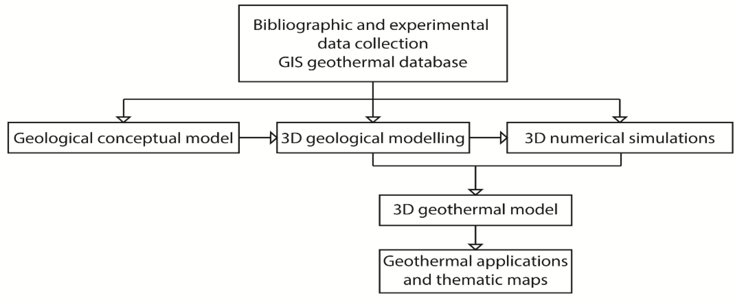
2. Methodology
3. Case History
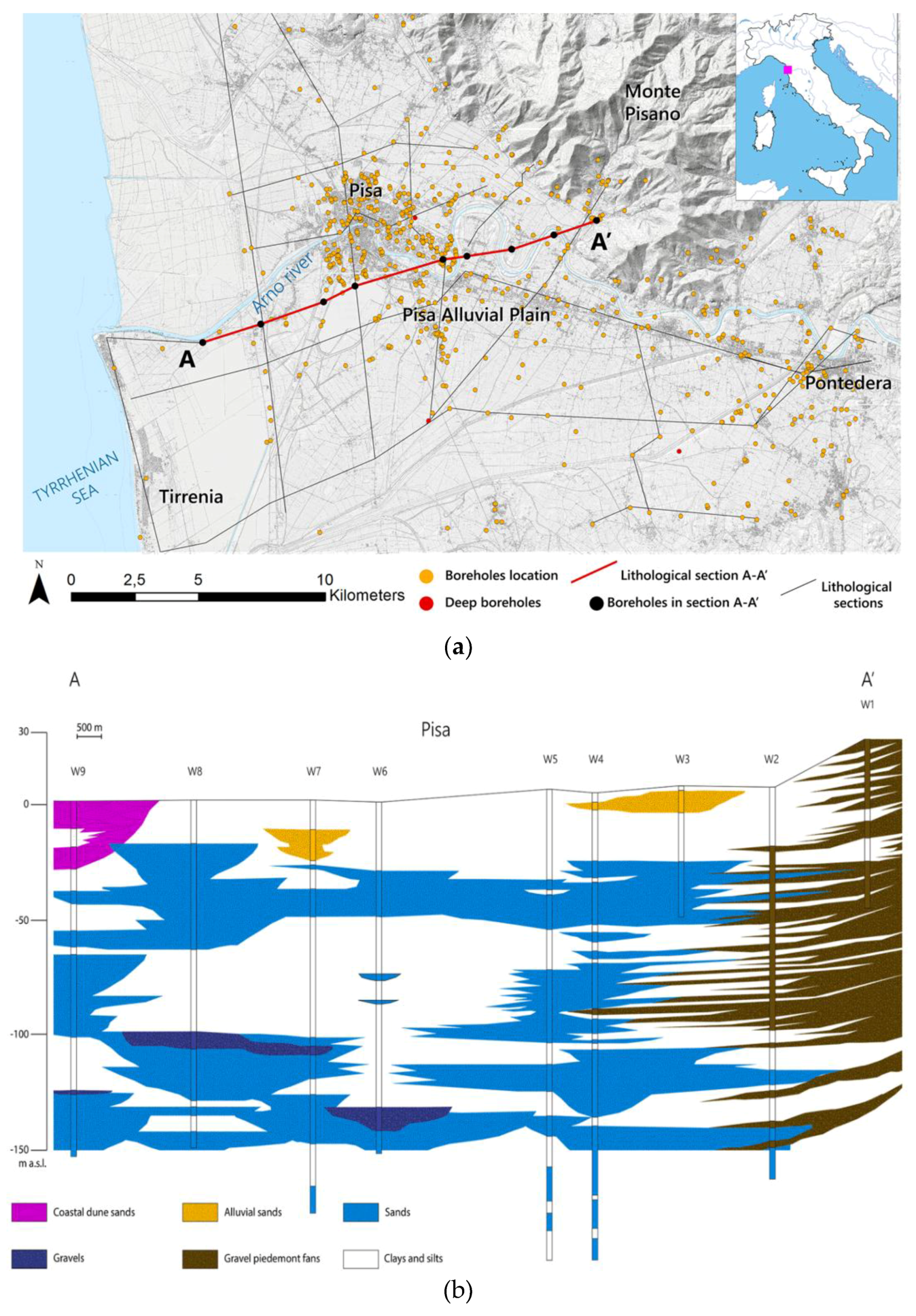
3.1. Database Setting, Data Screening, Collection, and Processing
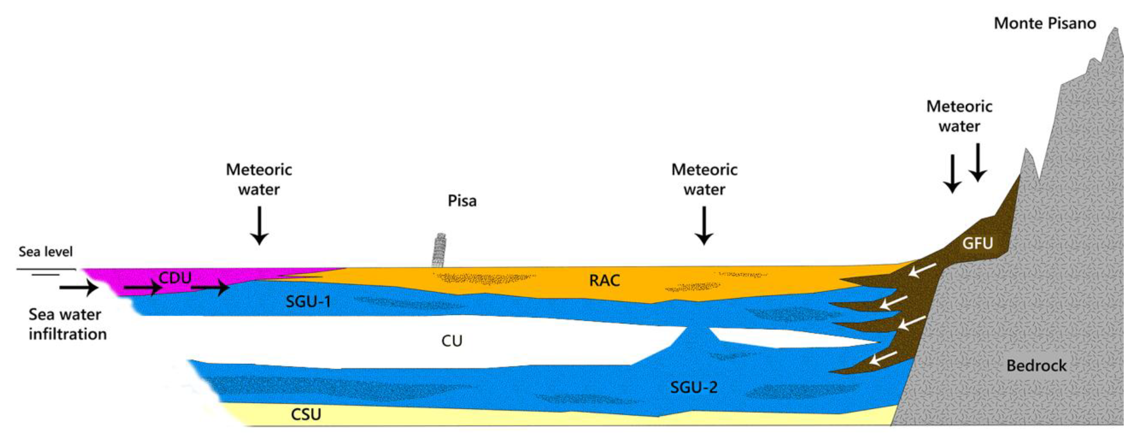
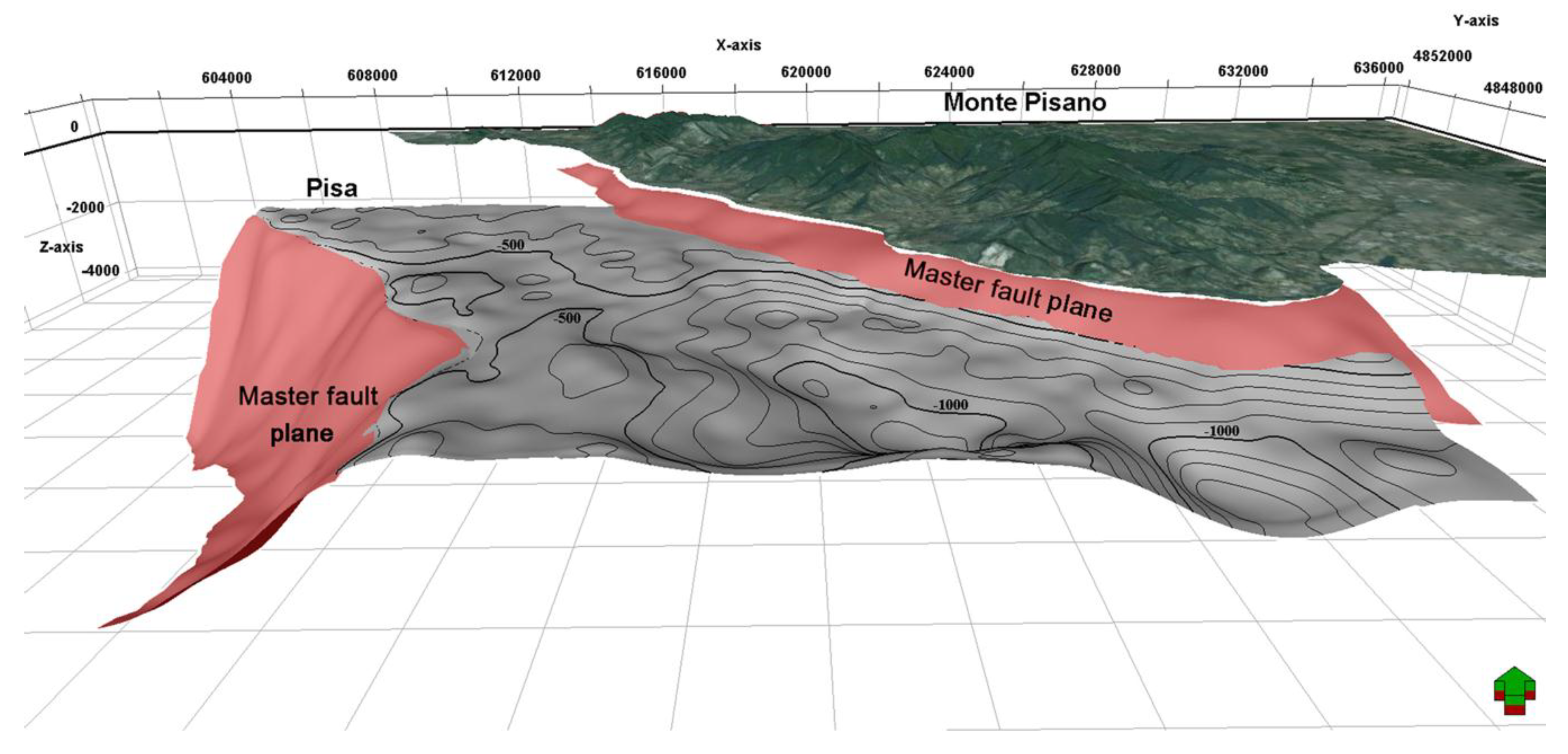
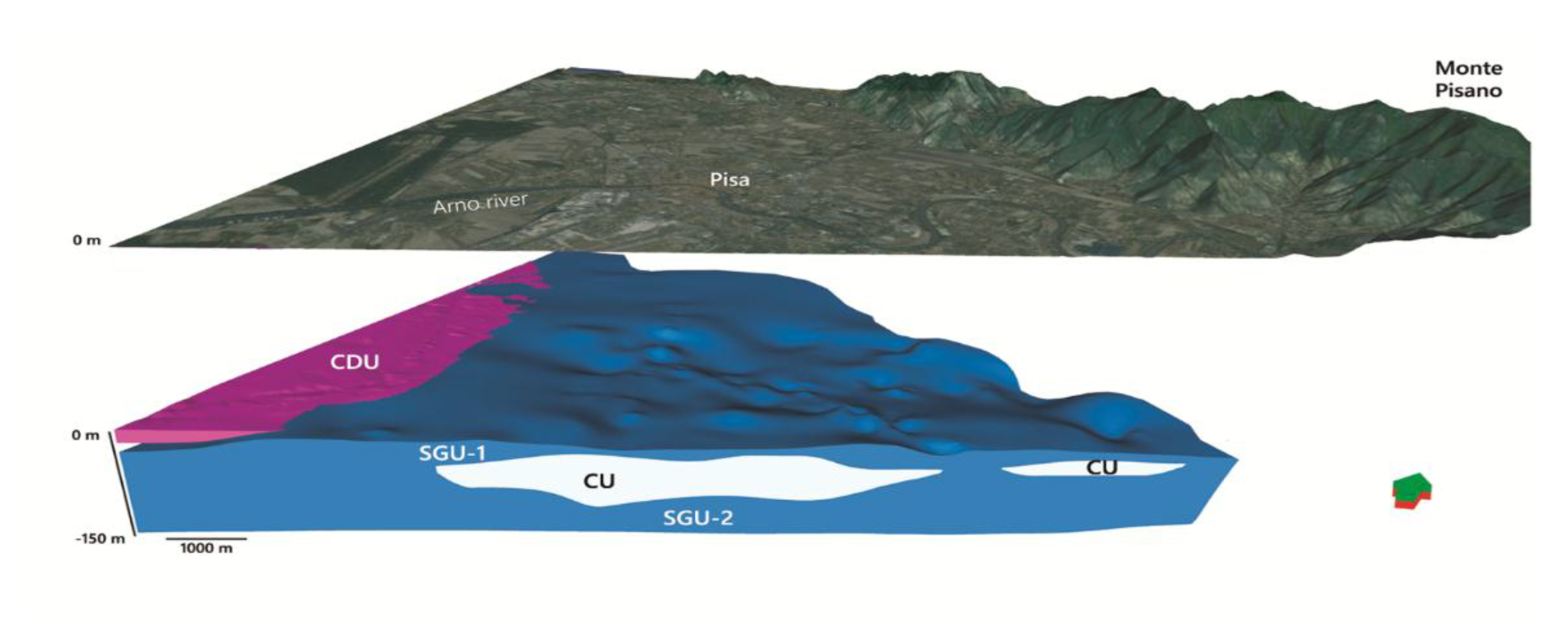
3.2. Geological Conceptual Model
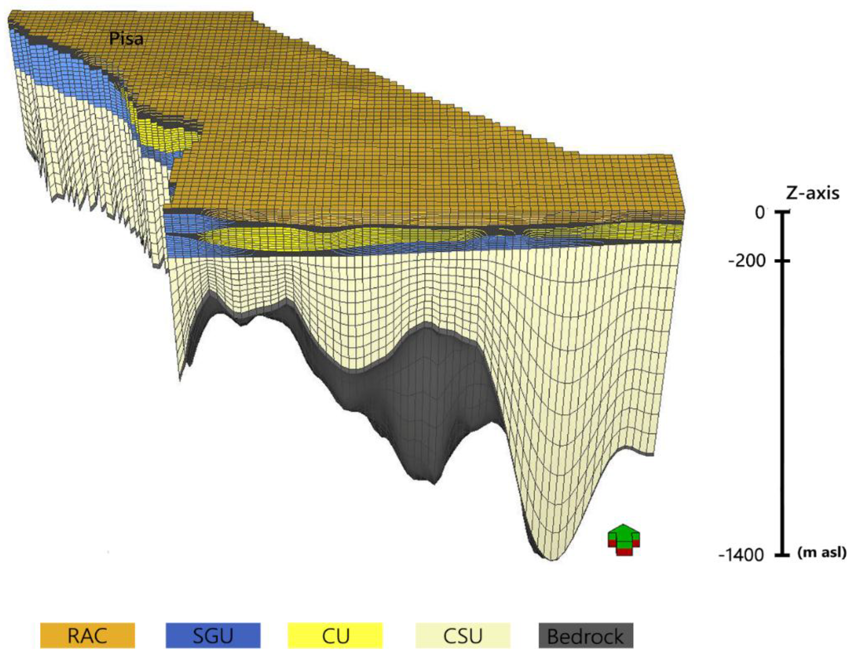
3.3. 3D Modeling
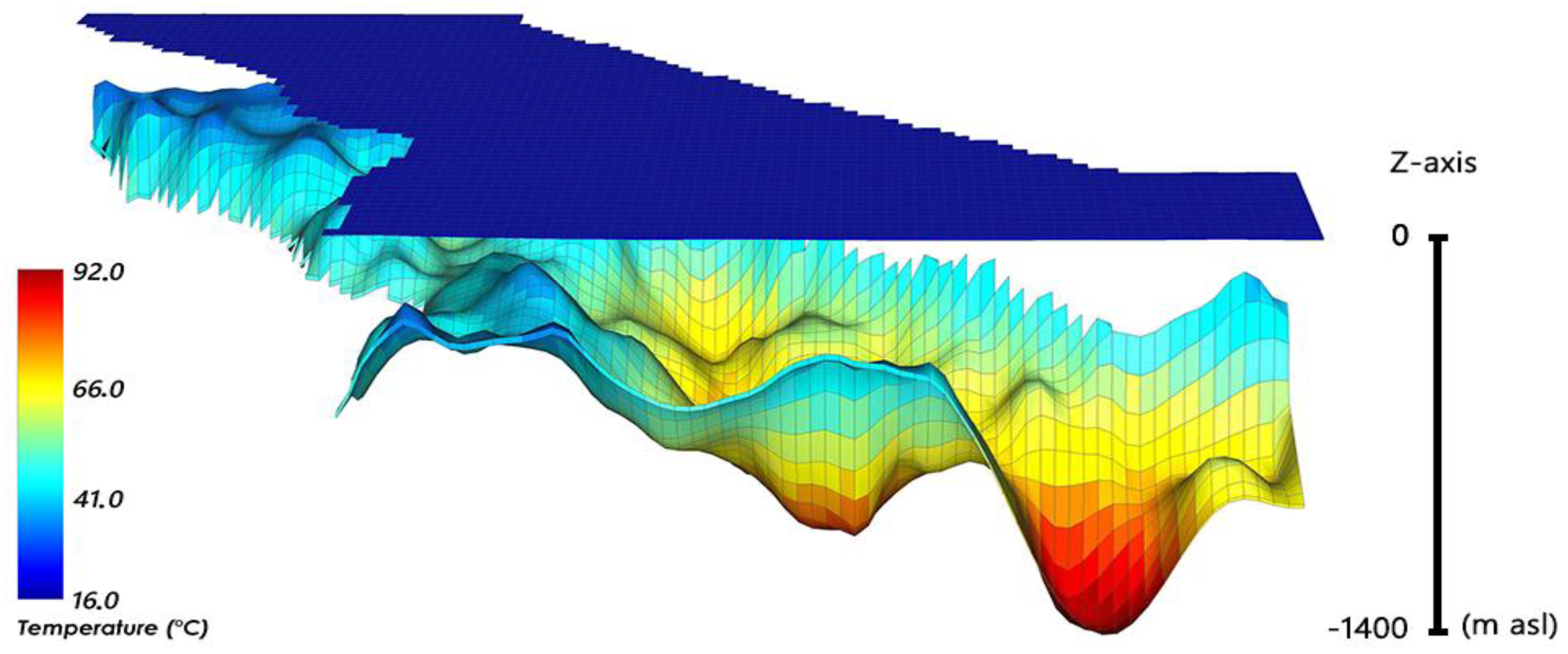
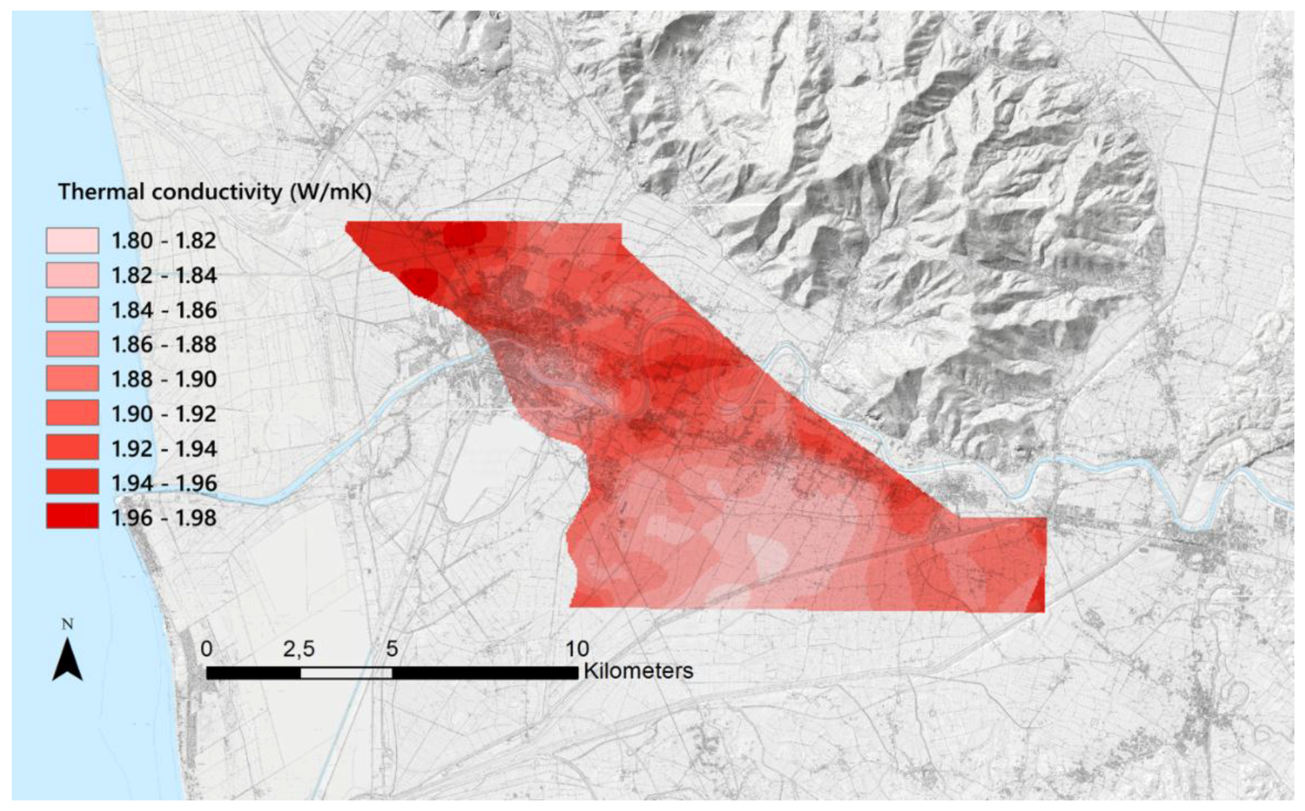
3.4. 3D Geothermal Modeling
4. Geothermal Applications
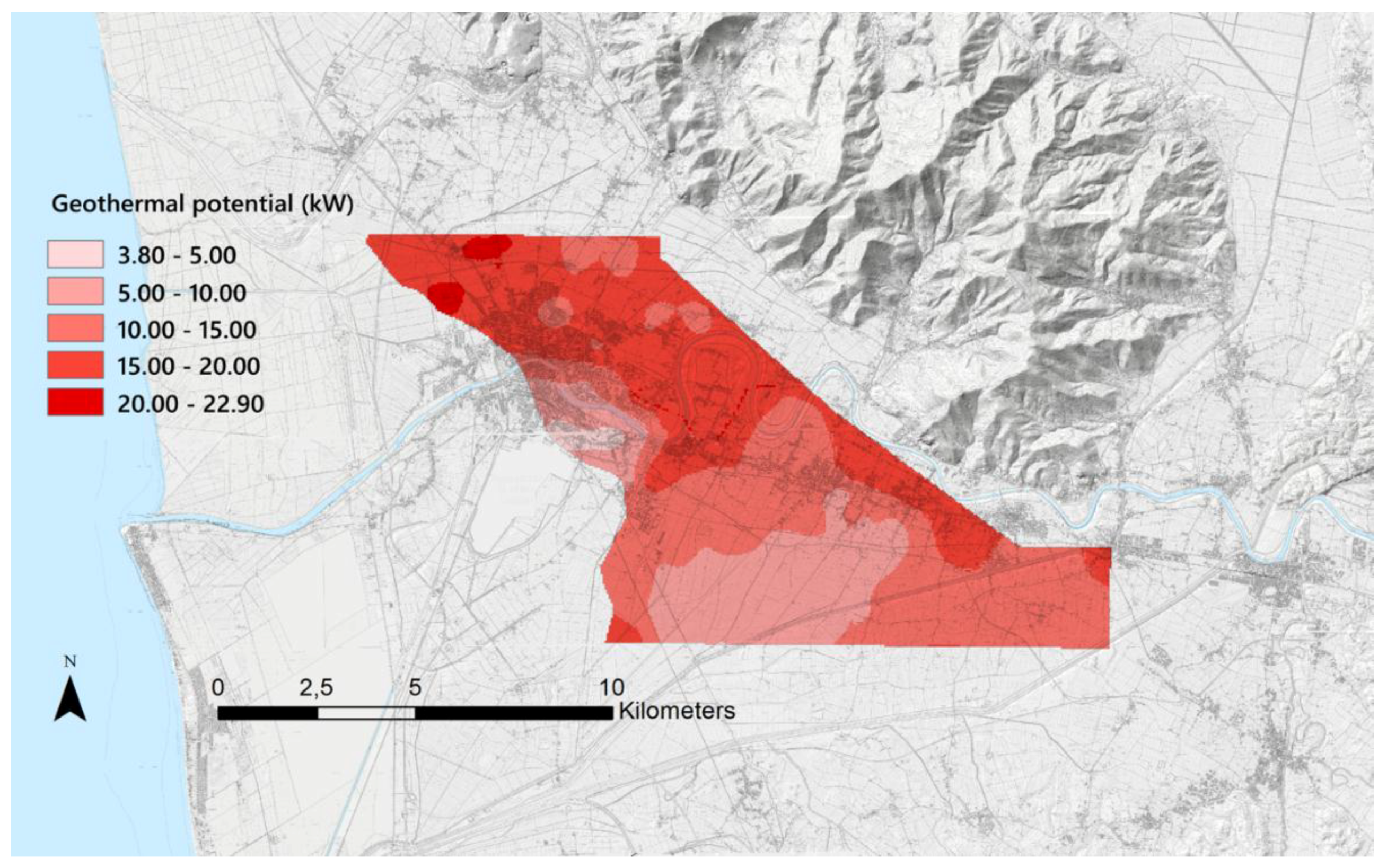
4.1. Evaluation of the Geothermal Potential for Open-Loop GHP Systems
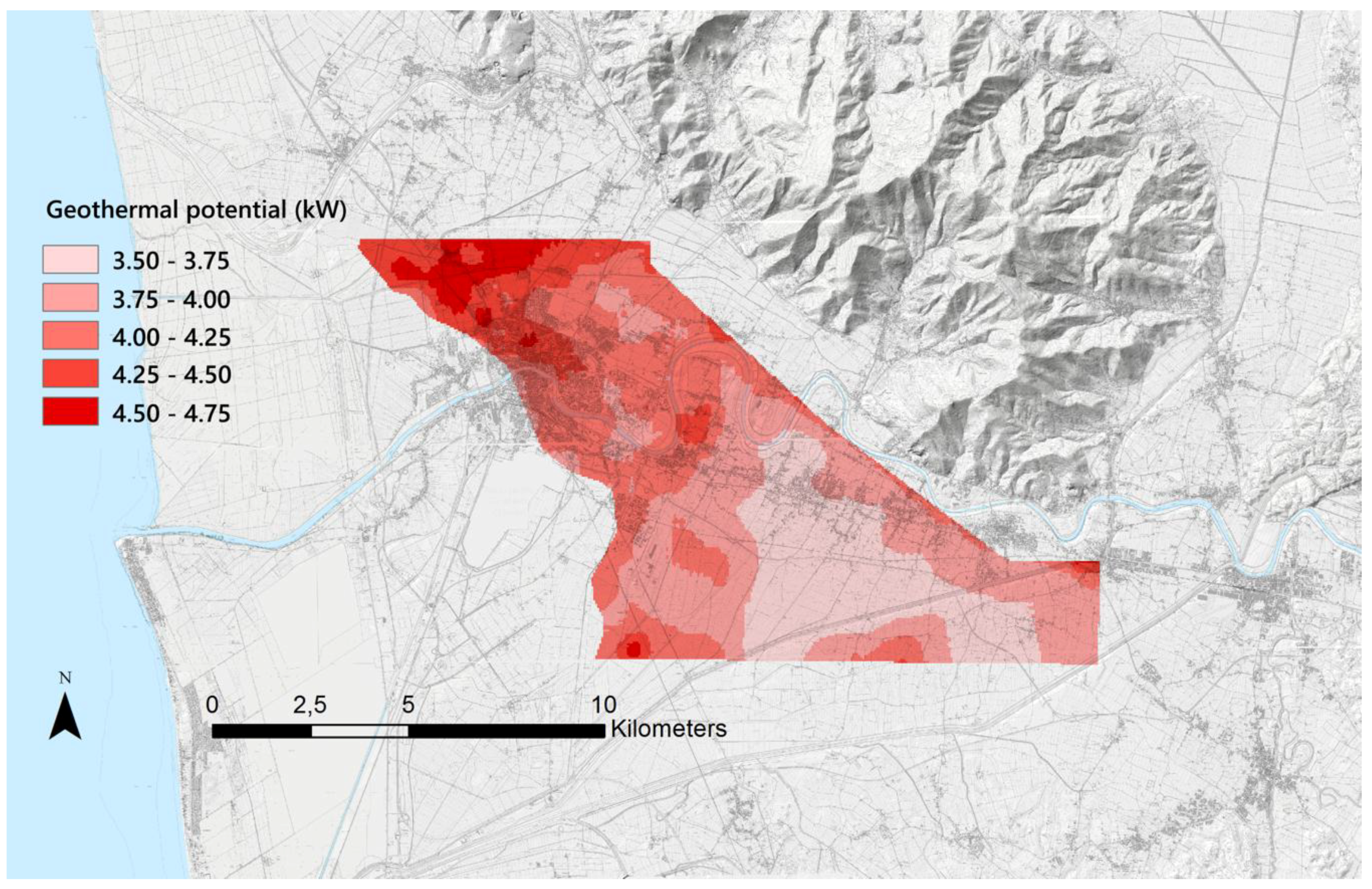
4.2. Evaluation of the Geothermal Potential for Closed-Loop GHP Systems
4.3. Evaluation of the Geothermal Potential for the Bedrock
4.4. Sustainability
5. Conclusions
Supplementary Materials
Author Contributions
Funding
Acknowledgments
Conflicts of Interest
Abbreviations
| 2D | Two-dimensional |
| 3D | Three-dimensional |
| a.s.l | Above Sea Level |
| bgl | Below Ground Level |
| BHE | Borehole Heat Exchanger |
| CDU | Coastal Dune Unit |
| CU | Clay Unit |
| CSU | Clay and Sands Unit |
| DTM | Digital Terrain Model |
| EED | Earth Energy Designer |
| EPSG | European Petroleum Survey Group |
| GeoDH | Geothermal District Heating systems |
| GFU | Gravel Fans Unit |
| GHP | Geothermal Heat Pump |
| GIS | Geographic Information System |
| GRS | Geodetic Reference System |
| G.POT | Geothermal POTential method |
| IDW | Inverse Distance Weighted interpolation |
| IFD | Integral Finite Difference |
| RAC | Recent Alluvial Cover |
| SGU | Sands and Gravels Unit |
| SGU-1 | Sands and Gravels upper Unit |
| SGU-2 | Sands and Gravels lower Unit |
| TOUGH | Transport of Unsaturated Groundwater and Heat |
| EOS | Equation of State |
| UTM | Universal Transverse of Mercator, cartographic projection |
| WGS | World Geodetic System |
References
- De la Cruz-Lovera, C.; Perea-Moreno, A.J.; de la Cruz-Fernández, J.L.; Alvarez-Bermejo, J.A.; Manzano-Agugliaro, F. Worldwide Research on Energy Efficiency and Sustainability in Public Buildings. Sustainability 2017, 9, 1294. [Google Scholar] [CrossRef]
- Pérez-Lombard, L.; Ortiz, J.; Pout, C. A review on buildings energy consumption information. Energy Build. 2008, 40, 394–398. [Google Scholar] [CrossRef]
- EU. Directive 2010/31/EU of the European Parliament and of the Council of 19 May 2010 on the Energy Performance of Buildings. Available online: http://eur-lex.europa.eu/legal-content/en/TXT/?uri=CELEX (accessed on 2 June 2018).
- Harvey, C.; Beardsmore, G.; Moeck, I.; Rüter, H. Geothermal Exploration: Global Strategies and Applications; IGA Service GmbH: Bochum, Germany, 2016. [Google Scholar]
- Chesnaux, R.; Lambert, M.; Fillastre, U.; Walter, J.; Hay, M.; Rouleau, A.; Daigneault, R.; Germaneau, D.; Moisan, A. Building a geodatabase for mapping hydrogeological features and 3D modeling of groundwater systems: Application to the Saguenay-Lac-St-Jean Region, Canada. Comput. Geosci. 2001, 37, 1870–1882. [Google Scholar] [CrossRef]
- Gogu, R.; Carabin, G.; Hallet, V.; Peters, V.; Dassargues, A. GIS-based hydrogeological databases and groundwater modeling. Hydrogeol. J. 2001, 9, 555–569. [Google Scholar] [CrossRef]
- Kaufmann, O.; Martin, T. 3D geological modeling from boreholes, cross-sections and geological maps, application over former natural gas storages in coal mines. Comput. Geosci. 2008, 34, 278–290. [Google Scholar] [CrossRef]
- Noorollahi, Y.; Itoi, R.; Fujii, H.; Tanaka, T. GIS integration model for geothermal exploration and well siting. Geothermics 2008, 37, 107–131. [Google Scholar] [CrossRef]
- Schiel, K.; Baume, O.; Caruso, G.; Leopold, U. GIS-based modelling of shallow geothermal energy potential for CO2 emission mitigation in urban areas. Renew. Energy 2016, 86, 1023–1036. [Google Scholar] [CrossRef]
- Ondreka, J.; Rusgen, M.I.; Stober, I.; Czurda, K. GIS-supported mapping of shallow geothermal potential of representative areas in south-western Germany—Possibilities and limitations. Renew. Energy 2007, 32, 2186–2200. [Google Scholar] [CrossRef]
- Akar, S.; Atalay, O.; Kuyumcu, O.C.; Solaroglu, U.Z.D.; Colpan, B.; Arzuman, S. 3D subsurface modeling of Gumuscoy Geothermal Area, Aydin, Turkey. Geotherm. Resour. Counc. Trans. 2011, 35, 669–676. [Google Scholar]
- Alkaraz, S.; Lane, R.; Spragg, K.; Milicich, S.; Sepulveda, F.; Bignall, G. 3D Geological Modelling Using New Leapfrog Geothermal Software. In Proceedings of the 36th Workshop on Geothermal Reservoir Engineering, Stanford University, Stanford, CA, USA, 31 January 31–2 February 2011. [Google Scholar]
- Alkaraz, S.; Chamberfort, I.; Pearson, R.; Cantwell, A. An Integrated Approach to 3-D Modelling to Better Understand Geothermal Reservoirs. In Proceedings of the World Geothermal Congress, Melbourne, Australia, 19–25 April 2015; pp. 1–7. [Google Scholar]
- Pearson, S.C.P.; Alcaraz, S.A.; White, P.A.; Tschritter, C. Improved visualization of reservoir simulations: Geological and fluid flow modeling of the Tauranga low-enthalpy geothermal system, New Zealand. Geotherm. Resour. Counc. Trans. 2012, 36, 1293–1297. [Google Scholar]
- Fulignati, P.; Marianelli, P.; Sbrana, A.; Ciani, V. 3D geothermal modelling of the Mount Amiata hydrothermal system in Italy. Energies 2014, 7, 7434–7553. [Google Scholar] [CrossRef]
- Bellani, S.; Grassi, S.; Squarci, P. Geothermal Characteristics of the Pisa Plain, Italy. In Proceedings of the World Geothermal Congress, Florence, Italy, 18–31 May 1995; Volume 2, pp. 1305–1308. [Google Scholar]
- Feng, G.; Xu, T.; Gherardi, F.; Jiang, Z.; Bellani, S. Geothermal assessment of the Pisa plain, Italy: Coupled thermal and hydraulic modeling. Renew. Energy 2017, 111, 416–427. [Google Scholar] [CrossRef]
- Gunnarsson, N. 3D Modeling in Petrel of Geological CO2 Storage Site. Master’s Thesis, Uppsala University, Uppsala, Sweden, 2011. [Google Scholar]
- Pruess, K.; Oldenburg, C.; Moridis, G. TOUGH2 User’s Guide, Version 2.0. Report LBNL-43134; Lawrence Livermore Laboratory: Berkeley, CA, USA, 1999; 198p.
- Narasimhan, T.N.; Witherspoon, P.A. An integrated finite difference method for analyzing fluid flow in porous media. Water Resour. Res. 1976, 12, 57–64. [Google Scholar] [CrossRef] [Green Version]
- Audigane, P.; Chiaberge, C.; Mathurin, F.; Lions, J.; Picot-Colbeaux, G. A workflow for handling heterogeneous 3D models with the TOUGH2 family of codes: Application to numerical modeling of CO2 geological storage. Comput. Geosci. 2011, 37, 610–620. [Google Scholar] [CrossRef]
- Shepard, D. A Two-Dimensional Interpolation Function for Irregularly-Spaced Data. In Proceedings of the 1968 ACM National Conference, New York, NY, USA, 27–29 August 1968; pp. 517–524. [Google Scholar]
- Balke, K.-D. Das Grundwasser als Energieträger. Brennstoff-Warme-Kraft 1977, 29, 191–194. [Google Scholar]
- Muffler, P.; Cataldi, R. Methods for regional assessment of geothermal resources. Geothermics 1978, 7, 53–89. [Google Scholar] [CrossRef]
- Pascucci, V.; Fontanesi, G.; Merlini, S.; Martini, I.P. Neogene Tuscan Shelf-Western Tuscany extension: Evidences of the early post-compressional deposits (Tyrrhenian Sea-Northern Apennines, Italy). Ofioliti 2001, 26, 187–196. [Google Scholar] [CrossRef]
- Sarti, G.; Rossi, V.; Giacomelli, S. The upper Pleistocene “Isola di Coltano sands” (Arno coastal plain, Tuscany Italy): Review of stratigraphic data and tectonic implications for the southern margin of the Viareggio basin. Atti Soc. Tosc. Sci. Nat. Mem. Pisa Italy Serie A 2015, 122, 75–84. [Google Scholar]
- Mariani, M.; Prato, R. I bacini neogenici costieri del margine tirrenico: Approccio sismico-stratigrafico. Mem. Soc. Geol. Ital. 1988, 41, 519–531. (In Italian) [Google Scholar]
- Trevisan, L.; Tongiorgi, E. Le Acque del Sottosuolo della Regione Pisana. “La Provincia Pisana”; Amministrazione Provinciale: Pisa, Italy, 1953; pp. 3–8. (In Italian)
- Dini, I. La Prima Falda Artesiana in Sabbia della Zona di Pisa; Comune e Provincia di Pisa: Pisa, Italy, 1976. (In Italian)
- Tongiorgi, M.; Rau, A.; Martini, I.P. Sedimentology of early-alpine, fluvio-marine, clastic deposits (Verrucano, Triassic) in the Monti Pisani (Italy). Sediment. Geol. 1997, 17, 311–332. [Google Scholar] [CrossRef]
- Fancelli, R. Tentativo di Ricostruzione Dell’andamento della Falda Artesiana tra i-30 ed i-50 m di Profondità nel Sottosuolo di Pisa e Dintorni; Rapporto CNR; Istituto Internazionale Ricerche Geotermiche: Pisa, Italy, 1984. (In Italian) [Google Scholar]
- Fancelli, R. Alcune Notizie sui Sedimenti Attraversati da Perforazioni per Ricerche D’acqua e Sulla Distribuzione Spaziale nel Sottosuolo Pisano delle Falde Acquifere; Rapporto CNR; Istituto Internazionale Ricerche Geotermiche: Pisa, Italy, 1984. (In Italian) [Google Scholar]
- Baldacci, F.; Bellini, L.; Raggi, G. Le risorse idriche sotterranee della pianura pisana. Atti Soc. Tosc. Sci. Nat. Mem. Pisa Italy Serie A 1994, 101, 241–322. (In Italian) [Google Scholar]
- Rossi, S.; Spandre, R. Caratteristiche idrochimiche della I falda artesiana in sabbia nei dintorni della città di Pisa. Acque sotterr. Fasc. 1994, 43, 51–58. (In Italian) [Google Scholar]
- Aguzzi, M.; Amorosi, A.; Sarti, G. Stratigraphic architecture of late quaternary deposits in the lower Arno plain (Tuscany, Italy). Geol. Romana 2005, 38, 1–10. [Google Scholar]
- Aguzzi, M.; Amorosi, A.; Castorina, F.; Ricci Lucchi, M.; Sarti, G.; Vaiani, C. Stratigraphic architecture and aquifer systems in the eastern Valdarno Basin, Tuscany. Geoacta 2006, 5, 39–60. [Google Scholar]
- Aguzzi, M.; Amorosi, A.; Colalongo, M.L.; Ricci Lucchi, M.; Rossi, V.; Sarti, G.; Vaiani, S.C. Late Quaternary climatic evolution of the Arno coastal plain (Western Tuscany, Italy) from subsurface data. Sediment. Geol. 2007, 202, 211–229. [Google Scholar] [CrossRef]
- Grassi, S.; Cortecci, G. Hydrogeology and geochemistry of the multi-layered confined aquifer of the Pisa plain (Tuscany-central Italy). Appl. Geochem. 2005, 20, 41–54. [Google Scholar] [CrossRef]
- Amorosi, A.; Lucchi, M.R.; Rossi, V.; Sarti, G. Climate change signature of small-scale parasequences from late glacial-Holocene transgressive deposits of the Arno valley fill. Paleogeogr. Paleoclimatol. Palaeoecol. 2009, 273, 142–152. [Google Scholar] [CrossRef]
- Sarti, G.; Rossi, V.; Amorosi, A. Influence of Holocene stratigraphic architecture on ground surface settlements: A case study from City of Pisa (Tuscany, Italy). Sediment. Geol. 2012, 281, 75–87. [Google Scholar] [CrossRef]
- Bonham-Carter, G.F. Geographic Information Systems for Geoscientists: Modeling with GIS; Pergamon Press: Oxford, UK, 1994; 398p. [Google Scholar]
- Carratori, L.; Ceccarelli Lemut, M.L.; Frattarelli Fischer, L.; Garzella, G.; Greco, G.; Grifoni Cremonesi, R.; Mazzanti, R.; Morelli, P.; Nencini, C.; Pasquinucci, M.; et al. Carta degli elementi naturalistici e storici della Pianura di Pisa e dei rilievi contermini, scala 1:50.000. In La Pianura di Pisa e i Rilievi Contermini la Natura e la Storia; Mazzanti, R., Ed.; Memorie della Società Geografica Italiana L: Rome, Italy, 1994; 491p. (In Italian) [Google Scholar]
- Belgiorno, M.; Marianelli, P.; Pasquini, G.; Sbrana, A. A contribution to the study of a Pisa alluvial plain sector for low-temperature geothermal assessment. Atti Soc. Tosc. Sci. Nat. Mem. Pisa Italy 2016, 123, 17–23. [Google Scholar] [CrossRef]
- Sbrana, A.; Pasquini, G.; Marianelli, P.; Bonciani, D.; Torsello, L. Geo4P-Geothermal Pilot Project Pisan Plain: Quantitative assessment of very low, low and medium temperature shallow geothermal resources. In Proceedings of the European Geothermal Congress, Technology and Best practice—Exploration and Planning, Strasbourg, France, 19–24 September 2016. [Google Scholar]
- Hinze, W.J.; Aiken, C.; Brozena, J.; Coakley, B.; Dater, D.; Flanagan, G.; Forsberg, R.; Hildenbrand, T.; Keller, G.R.; Kellogg, J.; et al. New standards for reducing gravity data: The North America gravity database. Geophysics 2005, 70, J25–J32. [Google Scholar] [CrossRef]
- Moritz, H. Geodetic Reference System 1980. Bull. Géod. 1980, 54, 395–405. [Google Scholar] [CrossRef]
- Banerjee, B.; Das Gupta, S.P. Gravitational attraction of a rectangular parallelepiped. Geophysics 1977, 42, 1053–1055. [Google Scholar] [CrossRef]
- Bott, M.H.P. The use of rapid digital computing methods for direct gravity interpretation of sedimentary basins. Geophys. J. Int. 1960, 3, 63–67. [Google Scholar] [CrossRef]
- Tuscany Region Website. Available online: http://www.regione.toscana.it/-/geoscopio (accessed on 14 May 2018).
- Hydrogeological Sector, Tuscany Region. Available online: http://www.sir.toscana.it (accessed on 14 May 2018).
- Zhu, K.; Blum, P.; Ferguson, G.; Balke, K.-D.; Bayer, P. The geothermal potential of urban heat islands. Environ. Res. Lett. 2010, 5, 044002. [Google Scholar] [CrossRef] [Green Version]
- Hurter, S.; Huenges, E.; Clauser, C.; Haenel, R. (Eds.) Atlas of Geothermal Resources in Europe; European Commission Office for Official Publications of the European Communities: Brussels, Belgium, 2002; 93p. [Google Scholar]
- Gazzetta Ufficiale della Repubblica Italiana, D.P.R. 142/93, Allegato A. Available online: http://efficienzaenergetica.acs.enea.it/doc/dpr412-93.pdf (accessed on 14 May 2018). (In Italian).
- VDI. VDI 4640 Thermal Use of the Underground. Blatt 1: Fundamentals, Approvals, Environmental Aspects; VDI: Düsseldorf, Germany, 2010. [Google Scholar]
- Casasso, A.; Sethi, R. G.POT: A quantitative method for the assessment and mapping of the shallow geothermal potential. Energy 2016, 106, 765–773. [Google Scholar] [CrossRef] [Green Version]


© 2018 by the authors. Licensee MDPI, Basel, Switzerland. This article is an open access article distributed under the terms and conditions of the Creative Commons Attribution (CC BY) license (http://creativecommons.org/licenses/by/4.0/).
Share and Cite
Sbrana, A.; Marianelli, P.; Pasquini, G.; Costantini, P.; Palmieri, F.; Ciani, V.; Sbrana, M. The Integration of 3D Modeling and Simulation to Determine the Energy Potential of Low-Temperature Geothermal Systems in the Pisa (Italy) Sedimentary Plain. Energies 2018, 11, 1591. https://doi.org/10.3390/en11061591
Sbrana A, Marianelli P, Pasquini G, Costantini P, Palmieri F, Ciani V, Sbrana M. The Integration of 3D Modeling and Simulation to Determine the Energy Potential of Low-Temperature Geothermal Systems in the Pisa (Italy) Sedimentary Plain. Energies. 2018; 11(6):1591. https://doi.org/10.3390/en11061591
Chicago/Turabian StyleSbrana, Alessandro, Paola Marianelli, Giuseppe Pasquini, Paolo Costantini, Francesco Palmieri, Valentina Ciani, and Michele Sbrana. 2018. "The Integration of 3D Modeling and Simulation to Determine the Energy Potential of Low-Temperature Geothermal Systems in the Pisa (Italy) Sedimentary Plain" Energies 11, no. 6: 1591. https://doi.org/10.3390/en11061591