A Class of Control Strategies for Energy Internet Considering System Robustness and Operation Cost Optimization


Research Institute of Information Technology, Tsinghua University, Beijing 100084, China
*
Author to whom correspondence should be addressed.
Energies 2018, 11(6), 1593; https://doi.org/10.3390/en11061593
Submission received: 28 May 2018
/
Revised: 12 June 2018
/
Accepted: 14 June 2018
/
Published: 18 June 2018
Abstract
:Aiming at restructuring the conventional energy delivery infrastructure, the concept of energy Internet (EI) has become popular in recent years. Outstanding benefits from an EI include openness, robustness and reliability. Most of the existing literatures focus on the conceptual design of EI and are lack of theoretical investigation on developing specific control strategies for the operation of EI. In this paper, a class of control strategies for EI considering system robustness and operation cost optimization is investigated. Focusing on the EI system robustness issue, system parameter uncertainty, external disturbance and tracking error are taken into consideration, and we formulate such robust control issue as a structure specified mixed control problem. When formulating the operation cost optimization problem, three aspects are considered: realizing the bottom-up energy management principle, reducing the cost involved by power delivery from power grid (PG) to microgrid (MG), and avoiding the situation of over-control. We highlight that this is the very first time that the above targets are considered simultaneously in the field of EI. The integrated control issue is considered in frequency domain and is solved by a particle swarm optimization (PSO) algorithm. Simulation results show that our proposed method achieves the targets.
1. Introduction
Over the last few decades, global warming, energy crises and ecological issues have promoted the research of renewable power generation and distributed energy networks [1,2]. For the integration of a variety of distributed energy resources (DERs), MGs play an important role [3,4]. In MGs, the produced power by renewable energy sources (RESs) including photovoltaic (PV) units and wind turbine generators (WTGs) has disadvantages such as low inertia, uncertainty, and dynamic complexity [5,6]. In addition, the output power of electrical loads depends on residents’ power usage customs and varies stochastically [7]. In MGs, to alleviate power imbalance, and to regulate voltage/frequency oscillation, the control of MGs is a subject of both practical and theoretical importance [8].
Following the principle of smart grids specializing in informatization and intellectualization of the existing power systems [9], and to solve the aforementioned challenges within the scenario of multiple interconnected MGs, the new concept of EI is proposed [10] and is considered to be an upgraded version of smart grid [11]. The definition and interpretation of EI are briefly outlined as follows. Inspired by cores of the Internet, the EI can be viewed as an Internet-style solution to energy related problems by integrating bi-directional flows of information and power [12]. Within the scope of EI, energy production and consumption are coordinated decentrally, such that open and peer-to-peer energy sharing is enabled. An iterative balance among power generation, storage and consumption shall be achieved in real time. In an EI scenario, multiple MGs are interconnected via energy router (ERs) [13], which are also known as energy hubs [14], or power routers [15]. Different from the top-down mode in the existing power systems, bottom-up is a fundamental energy management principle in EI [11]. To achieve such target, each individual MG in EI shall be able to regulate the power deviation with its local energy storage, generation and consumption devices with priority. If power balance in any MG is hard to be achieved autonomously, other MGs can send/absorb electrical energy to/from it via ERs, helping achieve its local power balance [11]. By scheduling and routing across energy cells in EI efficiently, secure and reliable power delivery can be achieved [12].
In the field of EI, when multiple MGs are interconnected, the related energy management and control issues are more complicated than the ones in isolated MG. Optimal control problems regarding energy management have been popular. For example, coordinated optimal control algorithm for smart distribution management system in multiple MGs is investigated in [16]. Applying a multi-objective stochastic optimization approach to solve the optimal energy management issues in MGs has been reported in [17]. To achieve an optimized operation of an off-grid MG, nonlinear droop relations are implemented in [18]. In [19], optimal control strategy for MG under both off-grid and grid-connected mode has been studied. Distributed control and optimization in DC MGs has been investigated in [20].
On the other hand, robust control problems in the fields of MG and EI have received much attention in the past few years. For instance, in [21], both and -synthesis approaches are utilized to regulate AC bus frequency deviations in an off-grid MG. A descriptor system approach has been applied in autonomous MGs to improve signal stability [22]. In [23], the issue of voltage control in an EI scenario is formulated as a non-fragile robust control problem regarding an uncertain stochastic nonlinear system, and it is solved via a linear matrix inequality approach. Robust load-frequency control (LFC) in a hybrid distributed generation system has been studied in [24].
For different optimal control problems mentioned in e.g., [16,17,18,19,20], a variety of optimization targets are considered to formulate the performance. For robust control problems discussed in e.g., [21,22,23,24], performance has been focused. When both and performances are considered simultaneously, the associated issues are called mixed control problems. The applications of mixed control theory in the field of MG have attracted much attention, and significant advances on this topic have been made. Some related research outputs are illustrated as follows. For an islanded AC MG, the problems of operation cost optimization and frequency regulation are formulated as a mixed control problem in deterministic systems in [25]. In [26], the robust mixed voltage control strategy is designed to improve signal stability and fault ride through capability for an islanded MG. It has been shown that the fixed structure mixed control technique can be used to obtain a coordinated vehicle-to-grid control and frequency controller for robust LFC in a smart grid [27]. A robust mixed based LFC of a deregulated power system including superconducting magnetic energy storage has been proposed in [28]. For other works regarding the application of mixed control into MGs, readers can refer to [29,30], etc. It is notable that, although a mixed control technique has been widely used in conventional power systems, there has been little work applying such control schemes into the field of EI.
When multiple MGs are interconnected via ERs, no matter if they are grid-connected or not, there are a variety of optimal and robust control problems worth considering. In this paper, we are concerned with the problems of controller design for EI considering system robustness and operation cost optimization. A series-shaped EI is studied in this article. Within the considered EI scenario, three MGs are interconnected successively and one MG has access to the main PG. In MGs, we assume that there exist the following elements: PV units, WTGs, fuel cells (FCs), hydrogen tanks (HTs), electrolyzers (ESs), micro-turbines (MTs), heat pumps (HPs), plug-in hybrid electric vehicles (PHEVs), diesel engine generators (DEGs), battery energy storage (BES) devices, flywheel energy storage (FES) devices, ERs and normal loads. The system of EI is formulated via a frequency domain approach. When the above robust and optimal control targets are considered simultaneously, PI controllers are utilized in ESs, MTs, HPs, PHEV, DEGs, the transmission line between and , and the transmission line between and . Then, we solve such control problem via a PSO algorithm [31]. Next, simulations demonstrate the usefulness and effectiveness of our proposed controller.
The importance and contribution of this work can be outlined as follows. As is mentioned above, some existing works only investigate either optimization of operation cost and energy management (e.g., [16,17,18,19,20]), or robustness against internal instability and external disturbances (e.g., [21,22,23,24]) of MG systems. In this paper, this is the very first time that both two aspects are considered simultaneously in the field of EI, rather than in conventional energy systems. The regulation of system robustness and tracking performance are formulated as a mixed control problem. Our work can be viewed as an extension as well as a generalized version for the ones focusing on single islanded or grid-connected MG. Comparing this paper with some existing ones adopting a time domain approach (e.g., [7,23,25]), our work formulated in the frequency domain has the advantage that it is convenient to be implemented in actual dynamic situations. With the proposed controller, the following targets are achieved simultaneously: (1) the system robustness against parameter uncertainty and external disturbance is achieved; (2) the tracking error is a controller to a relative low level; (3) the bottom-up energy management principle is achieved, such that an autonomous power balance in each MG is achieved with priority; (4) the cost involved by power delivery from PG to MG has been considered; (5) the controllable devices in MGs are utilized rationally, and the situation of over-control is avoided; (6) considering different preferences of the system manager, the importance of each control target can be adjusted by changing the size of its corresponding weighting coefficient; and (7) in simulation results, it is shown that the proposed controller performs better than the conventional ones do. It is highlighted that our work is of both theoretical and practical importance.
2. System Modelling
In this section, we focus on a series-shaped EI system with three ERs. Every component of the system is modelled with first order transfer function in frequency domain. Then, an explicit mathematical control system is obtained.
2.1. The Scenario of an EI
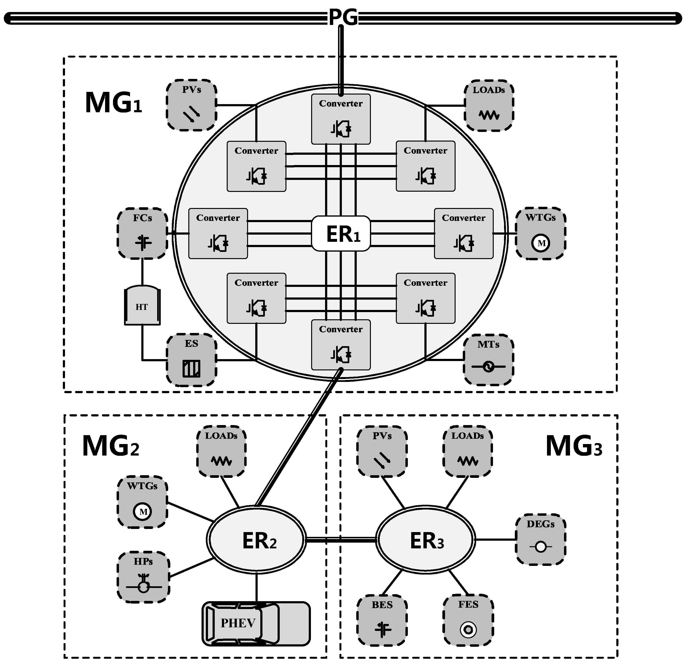
A series-shaped EI is studied in this article. , and are connected successively. In addition, we assume that is connected to PG. All of the ERs are designed to be based on AC bus lines. Figure 1 shows the topology of the studied EI system.
In , PV units, WTGs, loads, FCs, MTs, HTs and ESs are connected to via converters. The main power supply in is assumed to reply on power output by PV units and WTGs. If the power generation by PV units and WTGs is not enough for power consumption in , highly controllable power generators such as MTs and FCs are utilized to fill the power supply-demand gap. Whenever there exists superfluous energy in , ESs are used to covert electric energy into hydrogen, which is stored in HTs. Hydrogen can be used to generate power by FCs. Normal loads such as housings or factories have access to as well. In addition, is designed to have a connection to PG and .
is designed to have access to different components in , except for the requisite local loads. WTGs are utilized as the major power generators in . We assume that, in residential communities and cluster charging stations, large amounts of highly controllable HPs and PHEVs are connected to . When the power generation is larger than consumption in , the access of HPs and PHEVs shall be able to ensure the power balance of . Whenever suffers from a lack of electricity, power can be transmitted from and via and , respectively.
We assume that is only connected with and these two MGs are far away from each other. Thus, the dynamic response of power transmission line is slower than that of local devices in . Assuming that is sensitive to power deviation, responsive energy storage devices such as BES and FES devices are essential to keep its power balance. In addition, another kind of highly controllable power generator, DEGs, have connections with . PV units and loads are also included in .
2.2. Linearized Block Diagram
Power balance equation of , and can be expressed in Equations (1), (2) and (3), respectively:
In this paper, and are approximated by a first order transfer function [32], as is shown in Equations (4) and (5):
Considering the linear power versus frequency droop characteristics, is obtained by Equation (6):
Relative phase angle [rad] between PG and is obtained by Equation (7):
Let us denote as the relative phase angle and as line reactance. Consequently, is given by Equation (8):
We assume that BES and FES devices are equipped with internal controllers and respond to the AC bus frequency deviation [21]. and can be obtained by:
and are obtained by Equations (14) and (15):
Rapid or oversized power deviation may lead to instability of the AC bus frequency oscillation in MGs. With desired control strategies in , and , power balance in these MGs can be achieved, and instability of , and can be avoided. In this paper, PI controllers are utilized on ESs, MTs, HPs, PHEV, DEGs, the transmission line between and , and the transmission line between and . Then, we have:
where
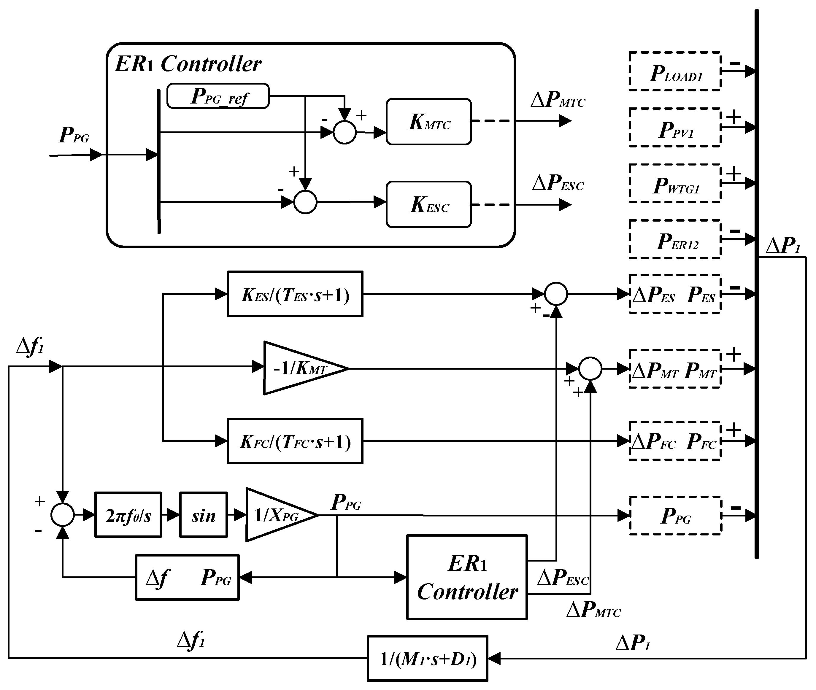
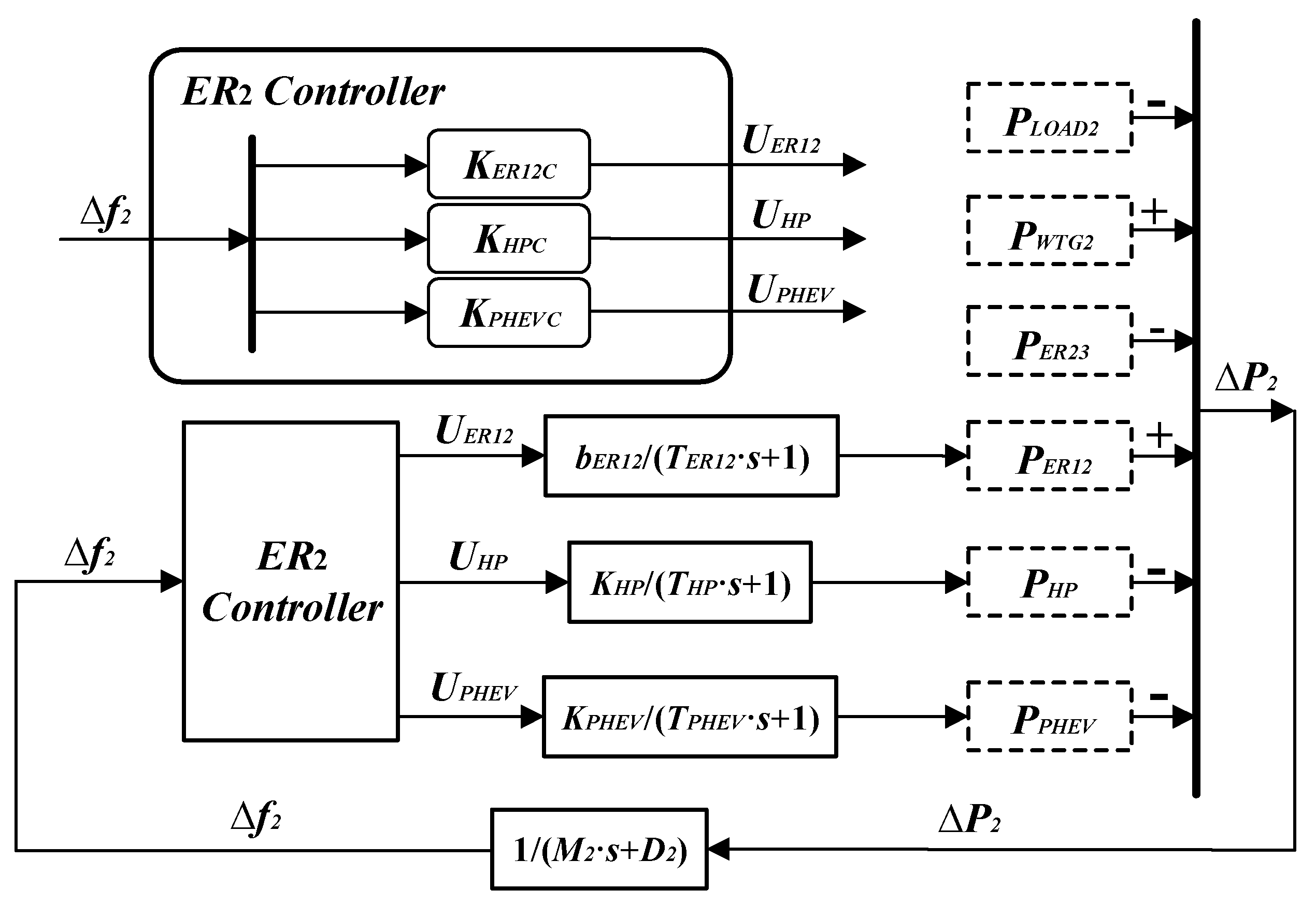
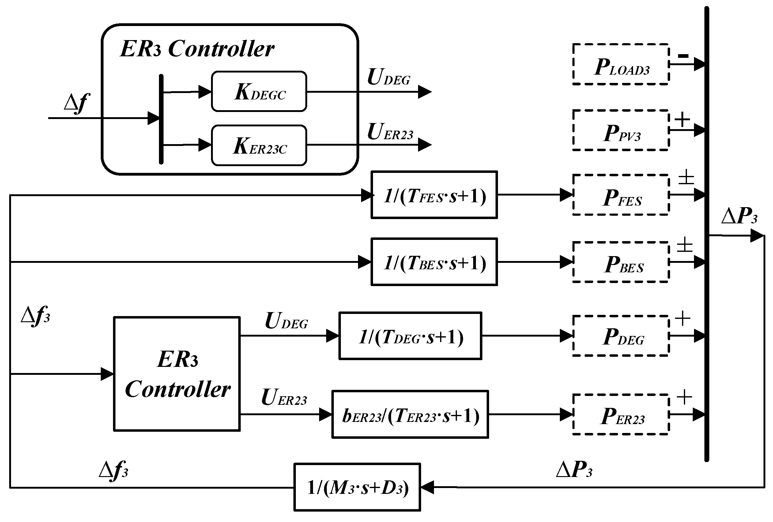
According to Equations (1), (4)–(8) and (16), the linearized block diagram of is illustrated in Figure 2. According to Equations (2), (9)–(11) and (16), the linearized block diagram of is illustrated in Figure 3. According to Equations (3), (12)–(16), the linearized block diagram of is illustrated in Figure 4.
Based on inverse Laplace transformation and the frequency-domain block diagram in Figure 2, Figure 3 and Figure 4, we are able to transform the studied EI system from Equations (1)–(16) into an explicit mathematical control system:
where is state vector, is output vector and is control output, expressed as:
The EI system Equation (16) is a multi-input-multi-output (MIMO) control system with the nominal plant and the controller .
We highlight that various topologies of EI (e.g., series-shaped, annular-shaped, star-shaped, etc.) can be formulated into mathematical systems in the form of Equation (17). Hence, the investigation to series-shaped EI and the obtained results can be extended and applied into generalized EI scenarios.
3. Problem Formulation and Solution.
In this section, the EI system robustness issue is formulated as the structure specified mixed control problem, whereas the operation cost management issue in EI is formulated as a multi-objective optimization problem. We consider such mixed robust and optimal control targets simultaneously, and we solve this control problem via a PSO algorithm [31].
3.1. Robust Control for EI
For a practical system, parameter measurement error and various power oscillation are inevitable, which brings system uncertainties [25,26]. In addition, power generated by PV units depends heavily on the condition of light intensity, and power generated by WTGs depends heavily on the condition of wind power. Moreover, varieties of power consumption devices can change the dissipation of power. Thus, external disturbance to the system shall be taken into consideration when designing robust controllers.
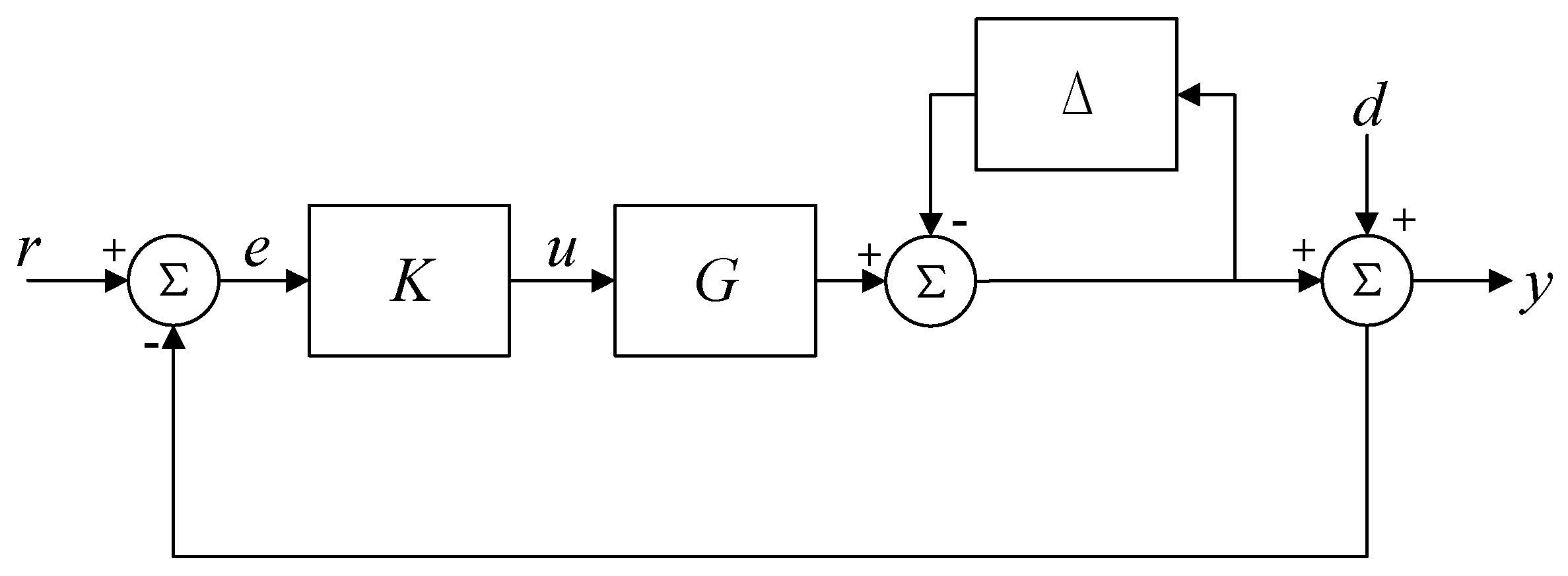
Considering a MIMO control system with external disturbances and system uncertainties, a nominal plant of the studied EI is denoted as , and represents the proposed controller. , , , and stand for reference input, tracking error, control output, external disturbance and system output, respectively. Inverse output multiplicative uncertainty [34], denoted as , is utilized to model system uncertainties. System robustness and tracking performance are formulated as and performance, respectively. The structure specified mixed control system is shown in Figure 5.
Based on the small gain theorem [35], a system with multiplicative uncertainties is stable if and only if Equation (18) holds:
where refers to the usual norm. Thus, we have
Based on Equation (19), the size of the system uncertainties is obtained by , which also implies the robust stability margin against the system uncertainties. Hence, the controlled system’s robust stability is maximized when is minimized. The robust control objective function is formulated as :
In addition to robust stability and disturbance attenuation, tracking performance should be optimized as well [36]. The objective function of tracking error is formulated as the integral of the squared error:
where stands for the usual norm, and is the tracking error, figured out by the inverse Laplace transformation of with and :
Thereby, considering system robustness, the structure specified mixed control objective function is obtained by given as follows:
3.2. Operation Cost Optimization
The operation cost of the studied system includes varieties of aspects among which three objective functions are identified below.
The first objective is to regulate the power transmission between every two connected MGs to a relatively low level. According to the bottom-up principle for EI, the autonomous power balance in each MG shall be achieved preferably. Equivalently, power transmission and are expected to be kept within a relatively small amount. According to the linearized block diagrams of and , the objective function can be formulated as :
The second objective function is focused on reducing the cost involved by power delivery from PG to MG. Within the scope of EI, the autonomous power generation is preferably nominated as the main energy supply source in a MG [10,11]. If a MG relies heavily on power exchange with PG to maintain its operation, it will not only violate the energy management principles of the EI, but also lead to expensive electricity purchasing cost. When economic benefit is concerned, both electricity price and the amount of power transmitted from PG to MG shall be considered. Normally, the electricity price varies over time by hours [37]. In this article, we focus on a time slot no more than one hour during which the electricity price is assumed to be constant. The economic cost involved by power delivery from PG to MG can be formulated as the 2-norm square of the product of electricity price and power transmitted from PG to :
where is the electricity price based on real-time electricity market. Thus, Equation (25) can be viewed as the second objective function.
The third objective function aims at reducing the additional cost involved by all the controllers utilized in the studied EI system. Although a stronger controller may lead to better performance, the probability of over-control is greatly increased. The situation of over-control will trigger additional costs for the operation of EI. The cost function is utilized to estimate the cost involved by the controllers:
where is the set of all the controllers in the studied EI system. According to Section 2, we have . By minimizing , the situation of over-control can be avoided effectively.
Taking three objective Equations (24)–(26) and the preference of the decision maker into consideration, the system operation cost function is formulated by:
where , and are weighting coefficients.
3.3. The Mixed Control Objective
The mixed control target is described by the sum of the structure specified mixed control objective function and the system cost optimization control objective, defined as
In this paper, our control target is to minimize , subject to:
In (29), and . is the set of all the proportion parameters, and . is the set of all the integral parameters, and . and are the minimum and maximum parameters of the proportion part of the controllers; and are the minimum and maximum parameters of the integral part of the controllers.
3.4. Solution to the Studied Control Problem
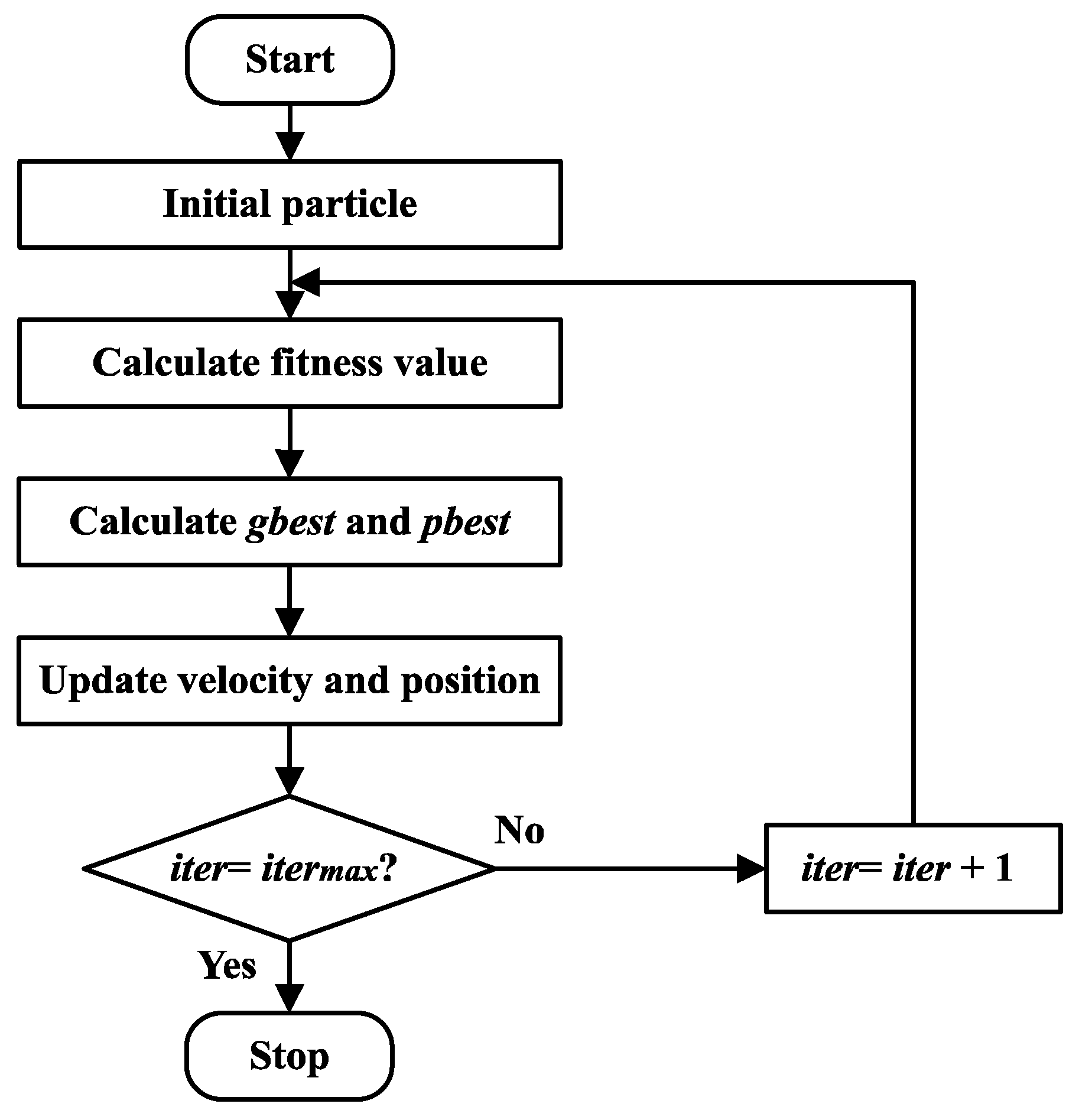
It is notable that the control problem described in Equations (28)–(29) can be solved by the PSO algorithm [31]. The flowchart of the PSO algorithm is shown in Figure 6, and the detailed implementation process is introduced as follows:
- Decide the numbers and the range of movement of the particles. Initialize them with random velocities and positions.
- Calculate the fitness value based on Equation (28) with the help of MATLAB (R2014b, MathWorks, Natick, MA, USA) μ-Analysis and Synthesis Toolbox.
- Calculate the best previously visited position and the global best position .
- Update the velocity and position of particle with the following equations:
- If is arrived, stop the circulation. Otherwise, go to process 2.
The simulation results are demonstrated in the next section.
4. Simulation Results and Analysis
In this section, some simulation results and analysis are given to verify the effectiveness of the proposed controller compared with the conventional ones.
4.1. Simulation Results under the Proposed Controller
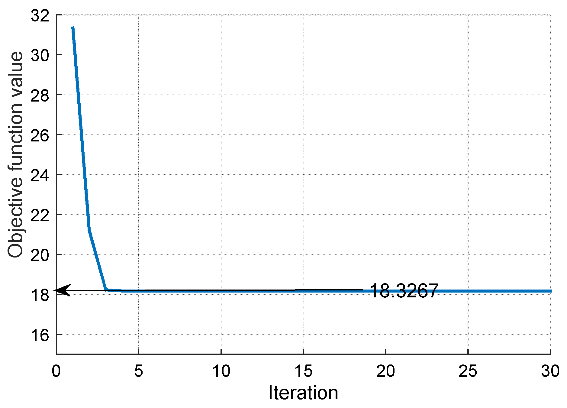
According to data in [21], [32] and [33], system parameters are given in Table 1. We assume that these parameters are valid for one hour only. In the next couple of hours, the values of system parameters shall be different and should be re-estimated. In this sense, our proposed method can be applied to any time period of a day without essential difficulty. For tracking performance, the reference input in Equation (22) is chosen to be . The parameters of PSO algorithm are: swarm size = 50; maximum iteration = 30; = 0.2; = 0.2; = 0.4 and = 0.9. According to the simulation results in Figure 7, the value of the optimized objective function is 18.3267.
The proposed mixed controller is:
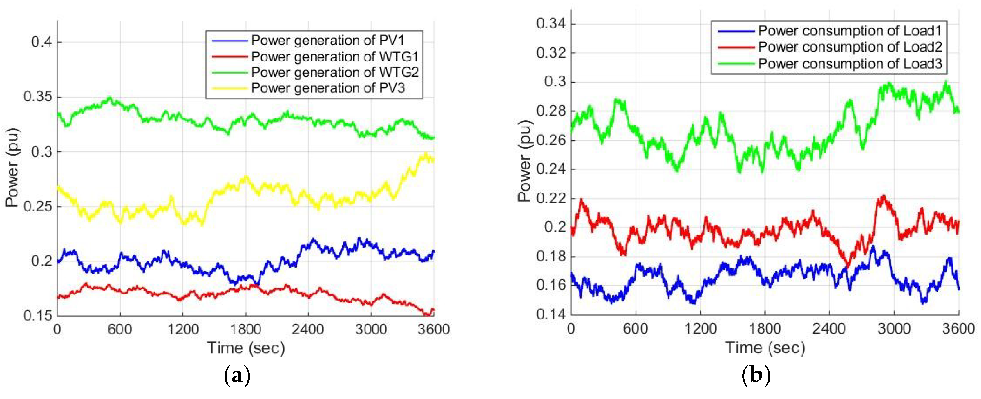
As is shown in Figure 8, the power generation by PV units and WTGs, as well as the power consumption of loads in the studied EI system, are assumed to be random in the investigated time period, simulated by forecasted models in [32].
The effect of the proposed method is compared with that of the conventional ones. Conventional methods include using only robust control, which minimizes in Equation (23) subject to Equation (29) and using only optimal control, which minimizes in Equation (27) subject to Equation (29).
4.2. Comparing the Proposed Controller with the Optimal Controller
Let the conventional method be only using optimal control strategies, which minimizes in Equation (27) subject to Equation (29). In this subsection, the parameter uncertainty is represented by a 50% increase of the original system parameters in Table 1, whereas a sudden increase of load power in three MGs (10% increase of , , ) is implemented as external disturbances.
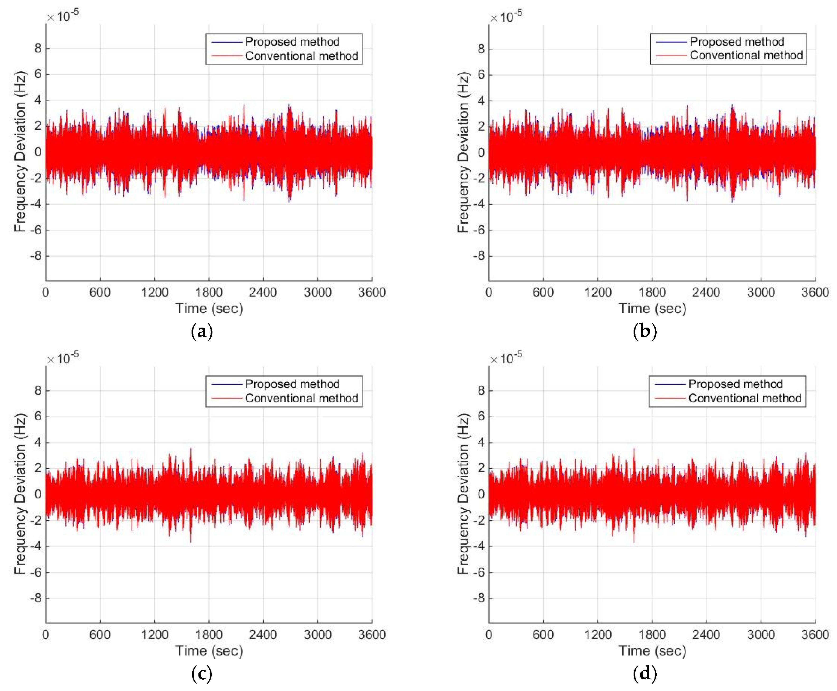
The controlled frequency deviation of obtained by both the proposed method and the conventional method are illustrated in Figure 9 including the following four situations: (a) without external disturbance or system parameter uncertainties; (b) with external disturbance only; (c) with system parameter uncertainties only; and (d) with both external disturbance and system parameter uncertainties. The frequency deviation of is relatively small, and the difference of the control effect of the proposed method and the conventional method is not obvious, which are due to the connection of to PG.
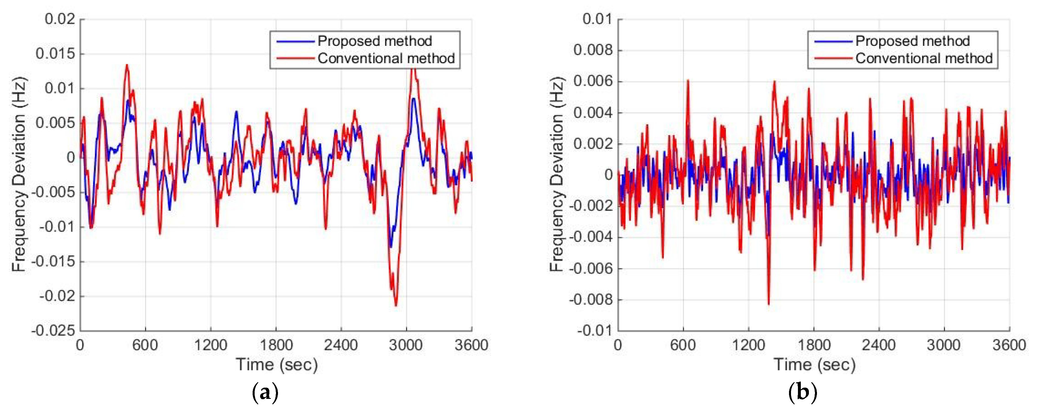
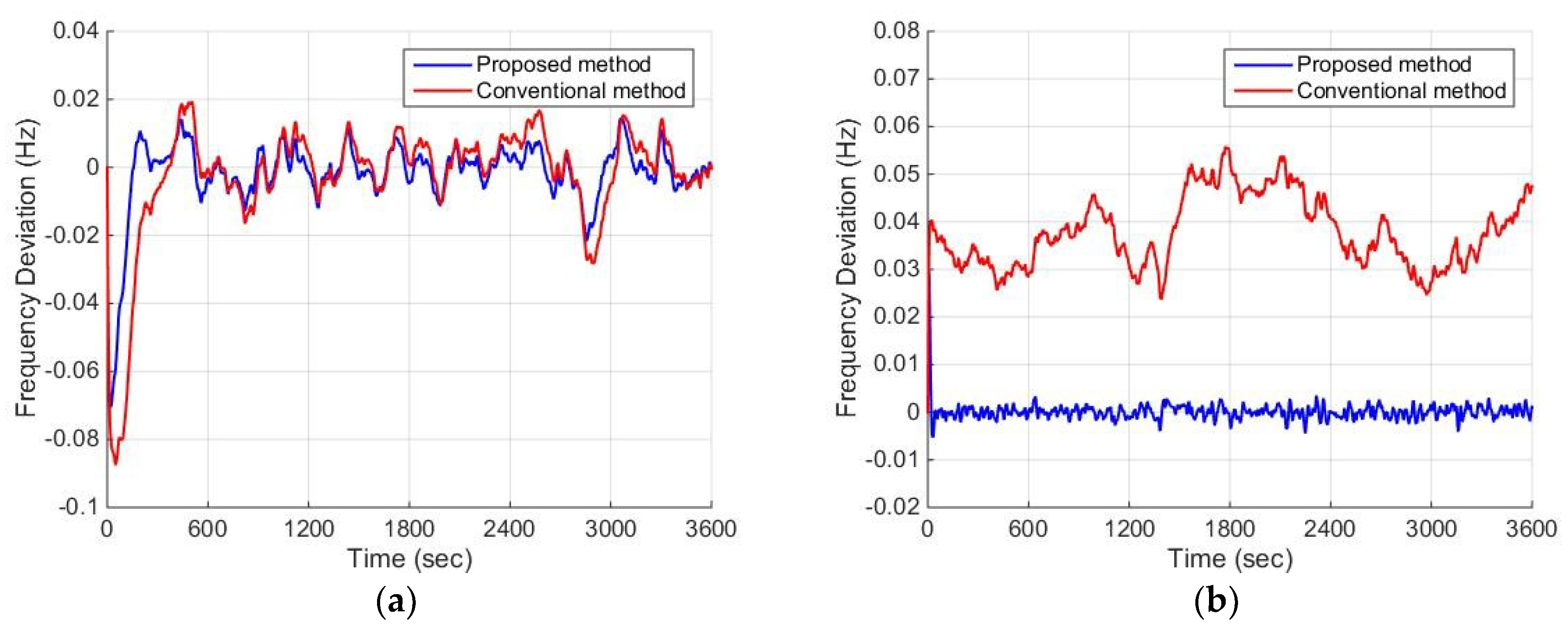
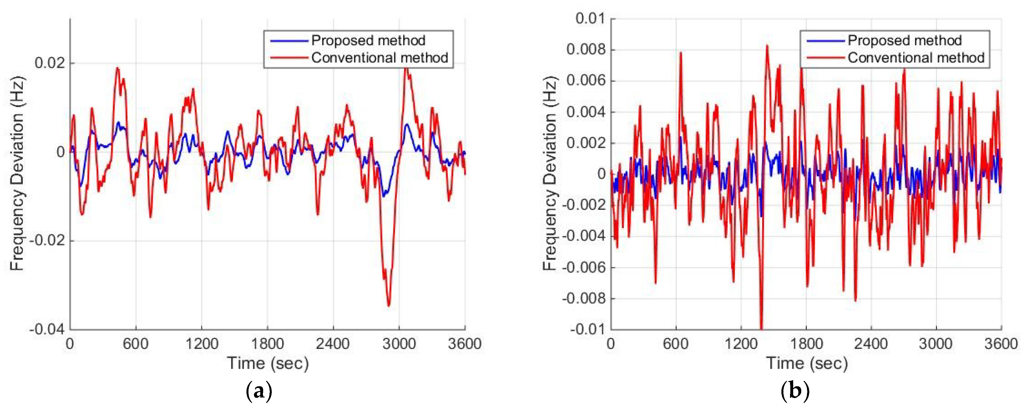
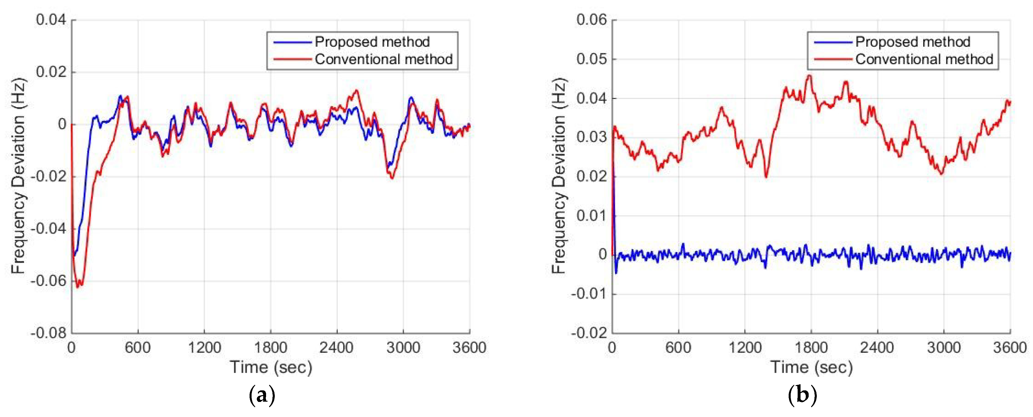
Frequency deviations of and without disturbance or uncertainties are illustrated in Figure 10. Obviously, the proposed method can stabilize the frequency of AC bus in and more efficiently. When only the external disturbance is considered, according to Figure 11, the proposed method has several advantages: the response speed is faster, the overshoot is smaller, and the transition period is shorter than the conventional method. When only system parameter uncertainty is considered, the frequency deviations of and are illustrated in Figure 12. The results show the effectiveness of the proposed controller. Moreover, under both external disturbance and system uncertainties, the studied EI system shows better performance with the proposed method, as is shown in Figure 13.
4.3. Comparing the Proposed Controller with the Robust Controller
Let the conventional method be only using robust control strategies in Equation (23) subject to Equation (29).
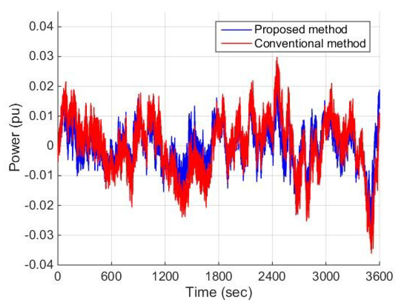
Figure 14 shows the power transmission between two adjacent MGs under the proposed controller and the conventional robust controller. Power transmission between PG and is illustrated in Figure 15. It is obvious that, using the proposed method, the transmission power between two adjacent MGs and that between PG and can be reduced effectively.
4.4. Some More Case Studeis
To show the impact of different weights on the objective function, two more cases are studied. The weight of a certain objective function can reflect the tendency of decision makers.
In Case 1, we assume that the physical distance between the interconnected MGs is long, leading to relatively high power transmission cost between MGs. Thus, the main energy exchange is preferably to be achieved between PG and MGs. In Case 2, decision makers are more inclined to reduce energy exchange with PG and control the whole EI system through the power flow between MGs.
A technique that combines the weighted sum method and the rank order centroid method [37] is utilized to determine the weights. The relative importance of the three objectives is reflected by the values of the weights, given by:
In our considered system, there are three MGs in total. Thus, . Two cases with different weights are studied as follows: in Case 1, we choose = 0.6110, = 0.2778, = 0.1112, whereas, in Case 2, we choose = 0.2778, = 0.6110, = 0.1112.
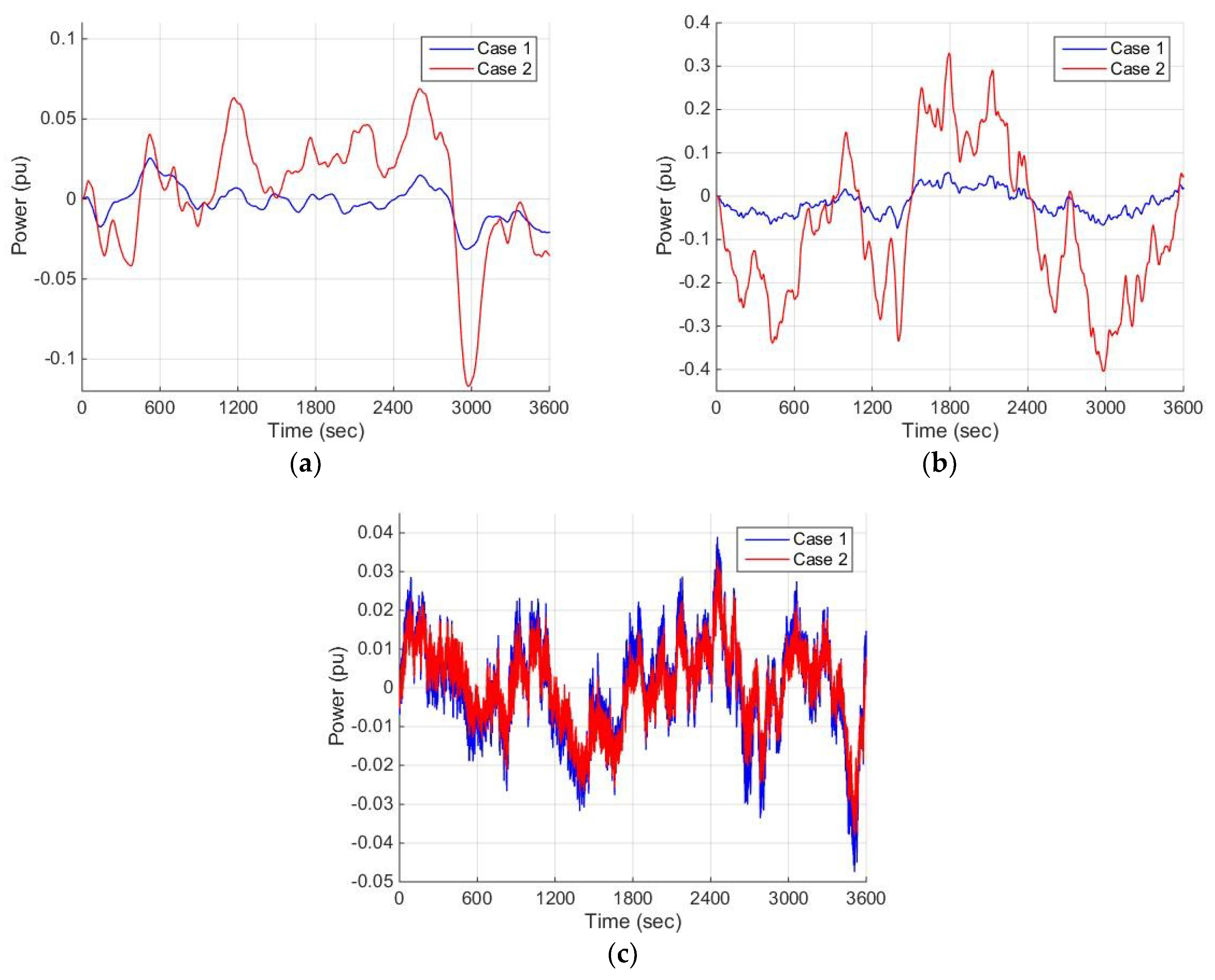
With the proposed method, the simulated results are illustrated in Figure 16.
From Figure 16a,b, it is obvious that power transmission via MGs under Case 1 is less than that under Case 2. From Figure 16c, we see that power transmission between PG and MGs under Case 1 is larger than that under Case 2. The above results show the feasibility of the impact of different weights on the objective function.
5. Conclusions
In this paper, a class of novel robust and optimal controller design for a dynamical series-shaped EI system has been presented. The robustness and operation cost optimization of the EI system are considered simultaneously. A PSO algorithm is applied to optimize the parameters of the proposed controller. Simulations show the effectiveness of the proposed method. For our future research, more authentic and complicated EI scenarios will be the focus, and the system communication time delay will be taken into consideration.
Author Contributions
The work presented here was carried out through the cooperation of all authors. H.H. and J.C. conceived the scope of the paper; C.H. and Y.Q. conceived the analysis and performed the simulations; H.H. and C.H. wrote the paper; J.C. acquired the funding and performed revisions before submission. All authors read and approved the manuscript.
Funding
This work was funded in part by the National Natural Science Foundation of China (Grant No. 61472200) and Beijing Municipal Science and Technology Commission (Grant No. Z161100000416004).
Conflicts of Interest
The authors declare no conflict of interest.
Nomenclature
| BES | Battery energy storage |
| Damping coefficient in | |
| Damping coefficient in | |
| Damping coefficient in | |
| DEG | Diesel engine generator |
| DER | Distributed energy resource |
| EI | Energy Internet |
| ER | Energy router |
| Energy router in | |
| Energy router in | |
| Energy router in | |
| ES | Electrolyzer |
| FC | Fuel cell |
| FES | Flywheel energy storage |
| Frequency deviation of | |
| Frequency deviation of | |
| Frequency deviation of | |
| HP | Heat pump |
| HT | Hydrogen tank |
| PI controllers of DEGs | |
| Gain of ESs | |
| PI controllers of ESs | |
| Gain of FCs | |
| Gain of HPs | |
| PI controllers of HPs | |
| Gain of MTs | |
| PI controllers of MTs | |
| Gain of PHEVs | |
| PI controllers of PHEVs | |
| LFC | Load-frequency control |
| Inertia constant in | |
| Inertia constant in | |
| Inertia constant in | |
| MG | Microgrid |
| The first microgrid | |
| The second microgrid | |
| The third microgrid | |
| MT | Micro-turbine |
| PG | Power grid |
| PHEV | Plug-in hybrid electric vehicle |
| PI | Proportional integral |
| PSO | Particle swarm optimization |
| PV | Photovoltaic |
| Exchange power of BES | |
| Output power of DEGs | |
| Output power of ESs | |
| Output power of FCs | |
| Exchange power of FES | |
| Output power of HPs | |
| Power consumption of load1 | |
| power consumption of load2 | |
| power consumption of load3 | |
| Output power of MTs | |
| Output power of PHEVs | |
| Output power of PV units in | |
| Output power of PV units in | |
| Output power of WTGs in | |
| Output power of WTGs in | |
| Power deviation of | |
| Power deviation of | |
| Power deviation of | |
| Change of | |
| Control outputs of ESs | |
| Change of | |
| Change of | |
| Control outputs of MTs | |
| RES | Renewable energy source |
| Time constants of BES devices | |
| Time constants of DEGs | |
| Time constants of ESs | |
| Time constants of FCs | |
| Time constants of FES devices | |
| Time constants of HPs | |
| Time constants of PHEVs | |
| Control outputs of DEGs | |
| Control outputs of HPs | |
| Control outputs of PHEVs | |
| WTG | Wind turbine generator |
| PI controller of transmission line between and | |
| PI controller of transmission line between and | |
| Power transmission between and | |
| Power transmission between and | |
| Power transmission between PG and | |
| Time constant of transmission line between and | |
| Time constant of transmission line between and | |
| Control output of transmission line between and | |
| Control output of transmission line between and |
References
- Bhattacharya, M.; Paramati, S.R.; Ozturk, I.; Bhattacharya, S. The effect of renewable energy consumption on economic growth: evidence from top 38 countries. Appl. Energy 2016, 162, 733–741. [Google Scholar] [CrossRef]
- Bilgen, S.; Kaygusuz, K.; Sari, A. Renewable energy for a clean and sustainable future. Energy Sources 2004, 26, 1119–1129. [Google Scholar] [CrossRef]
- Venkataramanan, G.; Marnay, C. A larger role for microgrids. IEEE Power Energy Mag. 2008, 6, 78–82. [Google Scholar] [CrossRef]
- Kroposki, B.; Lasseter, R.; Ise, T.; Morozumi, S.; Papathanassiou, S.; Hatziargyriou, N. Making microgrids work. IEEE Power Energy Mag. 2008, 6, 40–53. [Google Scholar] [CrossRef]
- Mathiesen, B.V.; Lund, H.; Connolly, D.; Wenzel, H.; Østergaard, P.A.; Möller, B.; Nielsen, S.; Ridjan, I.; Karnøe, P.; Sperling, K.; et al. Smart energy systems for coherent 100% renewable energy and transport solutions. Appl. Energy 2015, 145, 139–154. [Google Scholar] [CrossRef]
- Sreedharan, P.; Farbes, J.; Cutter, E.; Woo, C.; Wang, J. Microgrid and renewable generation integration: University of California, San Diego. Appl. Energy 2016, 169, 709–720. [Google Scholar] [CrossRef]
- Odun-Ayo, T.; Crow, M.L. Structure-preserved power system transient stability using stochastic energy functions. IEEE Trans. Power Syst. 2012, 27, 1450–1458. [Google Scholar] [CrossRef]
- Olivares, D.; Mehrizi-Sani, A.; Etemadi, A.; Canizares, C.; Iravani, R.; Kazerani, M.; Hajimiragha, H.A.; Gomis-Bellmunt, O.; Saeedifard, M.; Palma-Behnke, R.; et al. Trends in microgrid control. IEEE Trans. Smart Grid 2014, 5, 1905–1919. [Google Scholar] [CrossRef]
- Chakrabortty, A.; Ilić, M.D. Control and Optimization Methods for Electric Smart Grids; Springer: New York, NY, USA, 2012. [Google Scholar]
- Rifkin, J. The Third Industrial Revolution: How Lateral Power Is Transforming Energy, the Economy, and the World; Palgrave Macmillan: New York, NY, USA, 2013; pp. 31–46. [Google Scholar]
- Cao, J.; Yang, M. Energy Internet—Towards smart grid 2.0. In Proceedings of the Fourth International Conference on Networking & Distributed Computing, Los Angeles, CA, USA, 21–24 December 2013; pp. 105–110. [Google Scholar]
- Tsoukalas, L.H.; Gao, R. From smart grids to an energy Internet-assumptions, architectures and requirements. Smart Grid and Renew. Energy 2009, 1, 18–22. [Google Scholar]
- Han, X.; Yang, F.; Bai, C.; Xie, G.; Ren, G.; Hua, H.; Cao, J. An open energy routing network for low-voltage distribution power grid. In Proceedings of the 1st IEEE International Conference on Energy Internet, Beijing, China, 17–21 April 2017; pp. 320–325. [Google Scholar]
- Geidl, M.; Koeppel, G.; Favre-Perrod, P.; Klokl, B. Energy hubs for the futures. IEEE Power Energy Mag. 2007, 5, 24–30. [Google Scholar] [CrossRef]
- Boyd, J. An internet-inspired electricity grid. IEEE Spectr. 2013, 50, 12–14. [Google Scholar] [CrossRef] [Green Version]
- Wu, J.; Guan, X. Coordinated multi-microgrids optimal control algorithm for smart distribution management system. IEEE Trans. Smart Grid 2013, 4, 2174–2181. [Google Scholar] [CrossRef]
- Niknam, T.; Azizipanah-Abarghooee, R.; Narimani, M.R. An efficient scenario-based stochastic programming framework for multi-objective optimal micro-grid operation. Appl. Energy 2012, 99, 455–470. [Google Scholar] [CrossRef]
- Elrayyah, A.; Cingoz, F.; Sozer, Y. Construction of nonlinear droop relations to optimize islanded microgrid operation. IEEE Trans. Ind. Appl. 2015, 51, 3404–3413. [Google Scholar] [CrossRef]
- Zheng, X.; Li, Q.; Li, P.; Ding, D. Cooperative optimal control strategy for microgrid under grid-connected and islanded modes. Int. J. Photoenergy 2014, 2014, 1–11. [Google Scholar] [CrossRef]
- Zhao, J.; Dörfler, F. Distributed control and optimization in DC microgrids. Automatica 2015, 61, 18–26. [Google Scholar] [CrossRef]
- Bevrani, H.; Feizi, M.R.; Ataee, S. Robust frequency control in an islanded microgrid: H∞ and μ-Synthesis approaches. IEEE Trans. Smart Grid 2016, 7, 706–717. [Google Scholar] [CrossRef]
- Baghaee, H.R.; Mirsalim, M.; Gharehpetian, G.B.; Talebi, H.A. A generalized descriptor-system robust H∞ control of autonomous microgrids to improve small and large signal stability considering communication delays and load nonlinearities. Int. J. Electr. Power Energy Syst. 2017, 92, 63–82. [Google Scholar] [CrossRef]
- Hua, H.; Cao, J.; Yang, G.; Ren, G. Voltage control for uncertain stochastic nonlinear system with application to energy Internet: non-fragile robust H∞ approach. J. Math. Anal. Appl. 2018, 463, 93–110. [Google Scholar] [CrossRef]
- Singh, V.P.; Mohanty, S.R.; Kishor, N.; Ray, P.K. Robust H-infinity load frequency control in hybrid distributed generation system. Int. J. Elect. Power Energy Syst. 2013, 46, 294–305. [Google Scholar] [CrossRef]
- Hua, H.; Qin, Y.; Cao, J. A class of optimal and robust controller design for islanded microgrid. In Proceedings of the IEEE 7th International Conference on Power and Energy Systems, Toronto, ON, Canada, 1–3 November 2017; pp. 111–116. [Google Scholar]
- Baghaee, H.R.; Mirsalim, M.; Gharehpetian, G.B.; Talebi, H.A. A decentralized robust mixed H2/H∞ voltage control scheme to improve small/large-signal stability and FRT capability of islanded multi-DER microgrid considering load disturbances. IEEE Syst. J. 2017, 1–12. [Google Scholar]
- Vachirasricirikul, S.; Ngamroo, I. Robust LFC in a smart grid with wind power penetration by coordinated V2G control and frequency controller. IEEE Trans. Smart Grid 2014, 5, 371–380. [Google Scholar] [CrossRef]
- Shayeghi, H.; Jalili, A.; Shayanfar, H.A. A robust mixed H2/H∞ based LFC of a deregulated power system including SMES. Energy Convers. Manag. 2008, 49, 2656–2668. [Google Scholar] [CrossRef]
- Ngamroo, I. Robust coordinated control of electrolyzer and PSS for stabilization of microgrid based on PID-based mixed H2/H∞ control. Renew. Energy 2012, 45, 16–23. [Google Scholar] [CrossRef]
- Farsangi, M.M.; Song, Y.H.; Tan, M. Multi-objective design of damping controllers of FACTS devices via mixed H2/H∞ with regional pole placement. Int. J. Elect. Power Energy Syst. 2003, 25, 339–346. [Google Scholar] [CrossRef]
- Kennedy, J.; Eberhart, R. Particle swarm optimization. In Proceedings of the IEEE International Conference on Neural Networks, Perth, Australia, 27 November–1 December 1995; pp. 1942–1948. [Google Scholar]
- Li, X.; Song, Y.J.; Han, S.B. Study on power quality control in multiple renewable energy hybrid microgrid system. In Proceedings of the 2007 IEEE Lausanne Power Tech, Lausanne, Switzerland, 1–5 July 2007; pp. 2000–2005. [Google Scholar]
- Vachirasricirikul, S.; Ngamroo, I. Robust controller design of heat pump and plug-in hybrid electric vehicle for frequency control in a smart microgrid based on specified-structure mixed H2/H∞ control technique. Appl. Energy 2011, 88, 3860–3868. [Google Scholar] [CrossRef]
- Gu, D.W.; Petkov, P.H.; Konstantinov, M.M. Robust Control Design with MATLAB; Springer: New York, NY, USA, 2005. [Google Scholar]
- Jiang, Z.P.; Teel, A.R.; Praly, L. Small-gain theorem for ISS systems and applications. Math. Control Signals Syst. 1994, 7, 95–120. [Google Scholar] [CrossRef]
- Ho, S.J.; Ho, S.Y.; Hung, M.H.; Shu, L.S.; Huang, H.L. Designing structure-specified mixed H2/H∞ optimal controllers using an intelligent genetic algorithm IGA. IEEE Trans. Control Syst. Technol. 2005, 13, 1119–1124. [Google Scholar]
- Carpinelli, G.; Mottola, F.; Proto, D. A multi-objective approach for microgrid scheduling. IEEE Trans. Smart Grid 2017, 8, 2109–2118. [Google Scholar] [CrossRef]
Figure 1.
The studied series-shaped energy Internet (EI) system.

Figure 2.
The linearized block diagram of the first microgrid ().

Figure 3.
The linearized block diagram of the second microgrid ().

Figure 4.
The linearized block diagram of the third microgrid ().

Figure 5.
The control system of the studied EI with external disturbance and system uncertainties.

Figure 6.
The flowchart of the particle swarm optimization (PSO) algorithm.

Figure 7.
Objective function value.

Figure 8.
Local power generation and consumption; (a) power generation of photovoltaic (PV) units and wind turbine generator (WTGs); (b) power consumption of loads.
Figure 8.
Local power generation and consumption; (a) power generation of photovoltaic (PV) units and wind turbine generator (WTGs); (b) power consumption of loads.

Figure 9.
Frequency deviation of : (a) without disturbance or uncertainties; (b) with external disturbance; (c) with system parameter uncertainties; and (d) with external both disturbance and system parameter uncertainties.
Figure 9.
Frequency deviation of : (a) without disturbance or uncertainties; (b) with external disturbance; (c) with system parameter uncertainties; and (d) with external both disturbance and system parameter uncertainties.

Figure 10.
Frequency deviation without disturbance or uncertainties: (a) ; (b) .

Figure 11.
Frequency deviation with external disturbance: (a) ; (b) .

Figure 12.
Frequency deviation with system parameter uncertainties: (a) ; (b) .

Figure 13.
Frequency deviation with external disturbance and system parameter uncertainties: (a) ; (b) .
Figure 13.
Frequency deviation with external disturbance and system parameter uncertainties: (a) ; (b) .

Figure 14.
Power transmission between two adjacent MGs. (a) power transmission between and ; (b) power transmission between and .
Figure 14.
Power transmission between two adjacent MGs. (a) power transmission between and ; (b) power transmission between and .

Figure 15.
Power transmission between power grid (PG) and .

Figure 16.
Power transmission under Case 1 and Case 2: (a) between and ; (b) between and ; (c) between PG and .
Figure 16.
Power transmission under Case 1 and Case 2: (a) between and ; (b) between and ; (c) between PG and .


Table 1.
System parameters.
| Parameters | Value | Parameters | Value | Parameters | Value |
|---|---|---|---|---|---|
| 10 | 100 | 0.04 | |||
| 1 | 60 | 2 | |||
| 15 | 10 | 10 | |||
| 2 | 1.15 | 1.15 | |||
| 20 | 0.072 | 0.15 | |||
| 1.5 | 50 | 0.12 | |||
| 10 | 10 | - | - | ||
| 0.2 | 0.3 | - | - |
© 2018 by the authors. Licensee MDPI, Basel, Switzerland. This article is an open access article distributed under the terms and conditions of the Creative Commons Attribution (CC BY) license (http://creativecommons.org/licenses/by/4.0/).
Share and Cite
MDPI and ACS Style
Hua, H.; Hao, C.; Qin, Y.; Cao, J. A Class of Control Strategies for Energy Internet Considering System Robustness and Operation Cost Optimization. Energies 2018, 11, 1593. https://doi.org/10.3390/en11061593
AMA Style
Hua H, Hao C, Qin Y, Cao J. A Class of Control Strategies for Energy Internet Considering System Robustness and Operation Cost Optimization. Energies. 2018; 11(6):1593. https://doi.org/10.3390/en11061593
Chicago/Turabian StyleHua, Haochen, Chuantong Hao, Yuchao Qin, and Junwei Cao. 2018. "A Class of Control Strategies for Energy Internet Considering System Robustness and Operation Cost Optimization" Energies 11, no. 6: 1593. https://doi.org/10.3390/en11061593
Note that from the first issue of 2016, this journal uses article numbers instead of page numbers. See further details here.