Wind Farm Blockage and the Consequences of Neglecting Its Impact on Energy Production


1
DNV GL, Group Technology & Research, Power & Renewables, Bristol BS2 0PS, UK
2
DNV GL, Energy, Project Development, Melbourne 3008, Australia
3
DNV GL, Energy, Project Development, Glasgow G1 2PR, UK
*
Author to whom correspondence should be addressed.
Energies 2018, 11(6), 1609; https://doi.org/10.3390/en11061609
Submission received: 22 March 2018
/
Revised: 14 June 2018
/
Accepted: 15 June 2018
/
Published: 20 June 2018
Abstract
:Measurements taken before and after the commissioning of three wind farms reveal that the wind speeds just upstream of each wind farm decrease relative to locations farther away after the turbines are turned on. At a distance of two rotor diameters upstream, the average derived relative slowdown is 3.4%; at seven to ten rotor diameters upstream, the average slowdown is 1.9%. Reynolds-Averaged Navier-Stokes (RANS) simulations point to wind-farm-scale blockage as the primary cause of these slowdowns. Blockage effects also cause front row turbines to produce less energy than they each would operating in isolation. Wind energy prediction procedures in use today ignore this effect, resulting in an overprediction bias that pervades the entire wind farm.

1. Introduction
Fluid dynamic interaction between wind farm turbines changes the power production at each turbine relative to what it would produce in isolation. The effect can be large and therefore must be taken into account when estimating the energy production of a prospective wind farm. Despite all the attention this issue has received [1], energy production assessments (EPAs) continue to use, largely without challenge, an unsubstantiated assumption fundamental to turbine interaction calculations. These calculations assume that a turbine can only affect turbines located downstream—any influence on turbines upstream or laterally is almost always ignored.
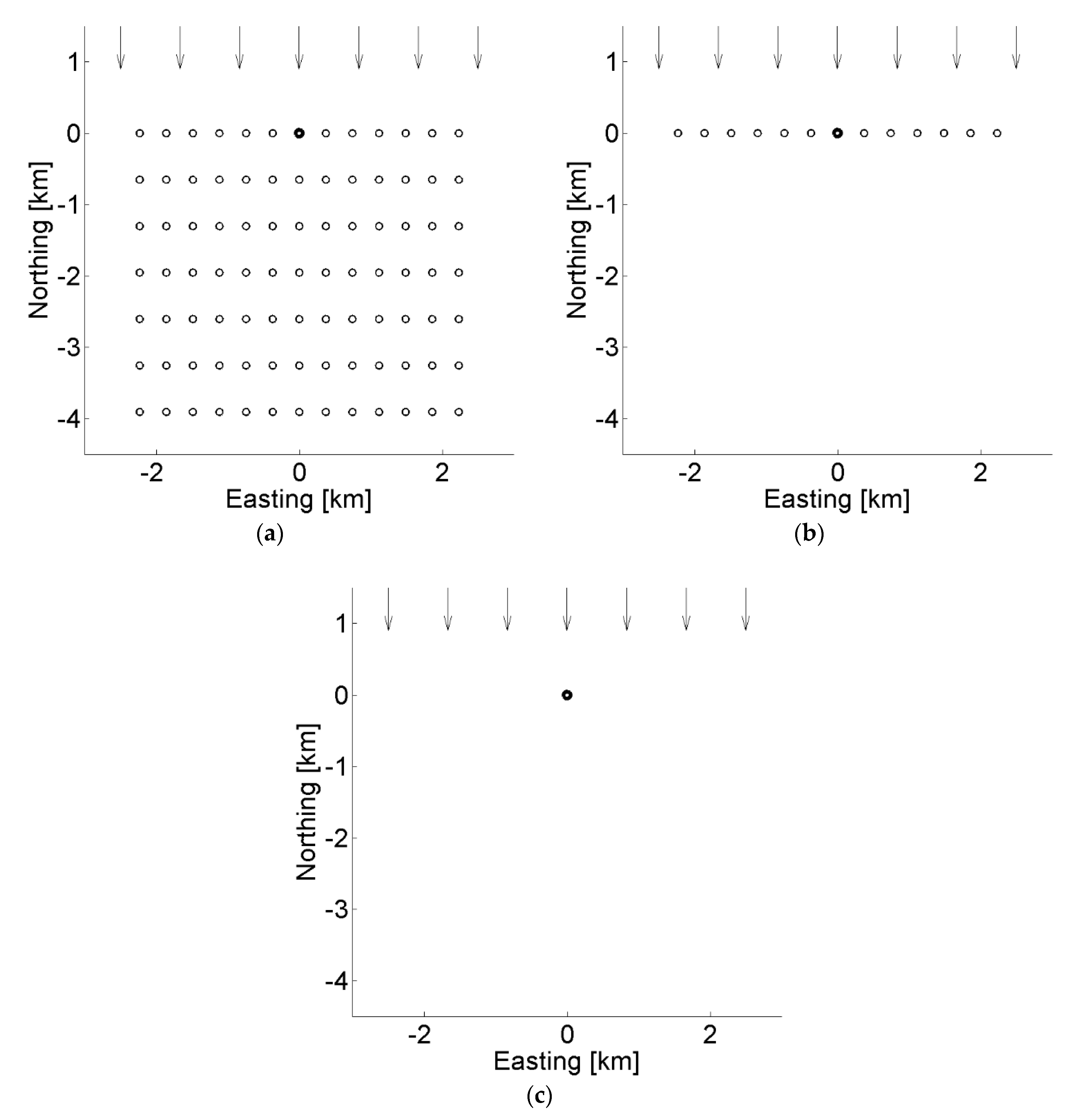
In this approach to calculating turbine interaction effects, a turbine on the upstream edge of a wind farm is impervious to the presence of the other wind farm turbines. In other words, the calculations assume that for northerly wind directions the highlighted wind turbine on the upstream row of the wind farm in Figure 1a will produce the same amount of energy as it would in a single row (Figure 1b), as well as when operating in isolation (Figure 1c). The approach further assumes that the upstream row in Figure 1a will produce at the same level as a single row of turbines in the same location (Figure 1b).
These assumptions define what we call the “wakes-only” approach to turbine interaction. Wake effects and their impact on turbines downstream are the only means of turbine interaction in this widely used approach. Accordingly, energy production changes due to turbine interaction are usually called “wake losses” [2], and models used to predict array efficiency are commonly referred to as “wake models” (Some commonly used wake models include a supplementary model targeting the impact of two-way coupling between the wind farm and atmosphere [3,4,5]. In these supplementary models, turbines still only influence conditions downstream; in turn, each turbine on the upstream edge of a modeled wind farm produces as if operating in isolation. Thus, this type of model also falls within the “wakes-only” category as defined herein).
Consistent with this approach, research on the fluid dynamic interaction between turbines has, until recently, focused almost exclusively on wakes. For example, wakes are the only type of turbine interaction considered in IEA Task 31, an ongoing international research collaboration to produce “best practice guidelines for wind farm flow modeling” [6]. Likewise, array losses are due to wake effects alone in most, if not all, treatments of the subject [7,8,9,10]. Many research articles, in fact, explicitly adopt wakes-only assumptions, with turbines on the upstream edges of wind farms referred to and treated as “free”, “freestream”, and/or “undisturbed” [2,6,9,11].
Yet the literature also includes indications of potential shortcomings in the wakes-only approach. In Ebenhoch [12], wind tunnel measurements and corresponding model predictions revealed a wind speed deficit upstream of a 105-turbine wind farm. The deficit was much larger and more far-reaching than could be attributed to a single turbine. The authors concluded that the observed upstream impact reduced the “amount of kinetic energy available for power extraction” and that the wakes-only “assumption is wrong”. As with many wind tunnel tests, the degree of applicability to full-scale is open to debate. The hub-to-hub distances in the wind tunnel were generally tight compared to modern wind farms (2.66 D laterally and 4 D streamwise, with D = rotor diameters), and there is also risk that the wind tunnel walls could influence the observed blockage. That said, large-eddy simulation results from two recent studies, [13,14], both showed significant wind speed decreases upstream of infinitely wide, full-scale wind farms. Allaerts [13] attributed the upstream flow decelerations to adverse pressure gradients induced by gravity waves. Wu [14] also attributed upstream deficits to gravity waves, but also to cumulative turbine induction, with the balance between the two influences strongly dependent on atmospheric conditions.
Other researchers have looked into whether turbine interaction can increase production from a single row of turbines perpendicular to the flow. Nishino [15], in an extension of earlier work with tidal turbines [16], showed Reynolds-Averaged Navier-Stokes (RANS) predictions of turbines producing up to 5% more energy when operating in a tightly spaced row (hub-to-hub distance of 1.5 D) as compared to when operating in isolation. In McTavish [17], wind tunnel measurements of three scaled-down turbines revealed production increases of a similar magnitude when the hub-to-hub distance was narrowed to 1.5 D. A flow model of the configuration yielded a similar result. Finally, Forsting [18] presented results from RANS simulations indicating that five turbines in a row perpendicular to the flow will outproduce the turbines in isolation by approximately 0.5% when the hub-to-hub spacing is 3.0 D. Unlike the RANS model, a vortex model predicted turbines in this configuration to have a negligible influence on each other for perpendicular flow. For non-perpendicular wind directions, however, both models predicted significant production variation along the row.
Finally, Mitraszewski [19] observed production variation along the unwaked edges of the Horns Rev 1 wind farm. Variation along unwaked perimeter turbines was consistently evident regardless of the wind direction, with turbines at the ends of the edges producing more than the turbines in the middle of those edges. A RANS simulation of a single wind direction at Horns Rev 1 yielded production variation along the unwaked edges resembling the observed variation [20]. Owner-operators of many wind farms have also reported seeing production variation among unwaked perimeter turbines similar to that observed at Horns Rev [21]. The authors of [19] attributed the production variation to Coriolis effects and in turn surmised that the variation represented a redistribution of energy at the wind farm rather than a net loss or gain.
Despite the emerging evidence of extra-wake turbine interaction, the wakes-only approach remains well-entrenched within EPA practices. A shift away from this approach may require more evidence—particularly from real wind farms—and moreover, a consensus understanding of how these interactions affect wind farm energy production.
Assuming turbine interaction is limited to wake effects makes accounting for the interaction more straightforward and less computationally expensive. It lets energy production modelers avoid, or at least greatly simplify, calculations of the two-way coupling that occurs between wind farm and atmosphere. Further, the wakes-only approach has led to the widespread adoption of parabolic wind farm flow models (i.e., wake models) with their concomitant advantages in computation speed. Thus, the wakes-only assumption clearly offers convenience; the empirical and physical justification for its use, however, is less clear. In fact, the authors are not aware of any direct evidence substantiating this long-held assumption.
In the absence of substantiation, there is heightened risk that EPAs are neglecting influences that have a material impact on wind farm energy production. This could potentially lead to bias in energy production estimates and less-efficient wind farm designs. The aim of this research is to investigate the validity of the wakes-only assumption and explore the consequences should the assumption prove to be false. To this end, we focus on wind speed measurements and RANS simulations at three large wind farms. The paper provides the details of these analyses and discusses the results. After highlighting the implications of the findings, we recommend changes to currently accepted practices for estimating wind farm production.
2. Measurements
The three wind farm projects at the center of this investigation are located onshore and consist of modern wind turbines with rotor diameters in excess of 80 m. The projects also share a rare combination of three features that together offer insight into the upstream influence of a wind farm:
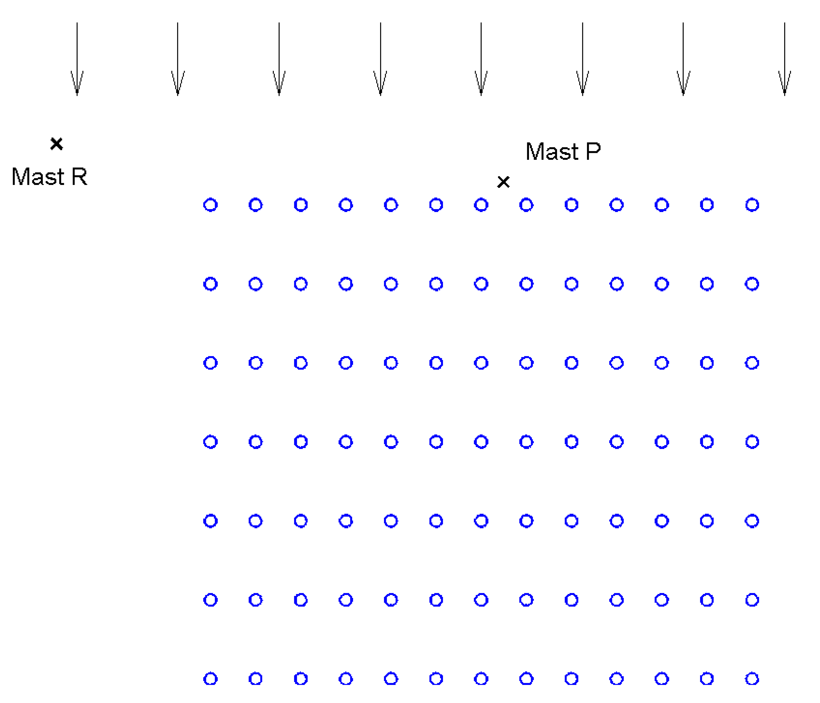
- At least one meteorological mast located just upstream of the wind farm for the prevailing wind direction (e.g., Mast P in Figure 2).
- At least one additional mast located much farther upstream or lateral to the wind farm for the prevailing wind direction (e.g., Mast R in Figure 2).
- The masts have been taking wind speed and direction measurements concurrently before and after the wind farm commercial operation date (COD).
We refer to Mast P in Figure 2 as a “perimeter mast” and Mast R as a “reference mast”. The objective of the data analysis is to determine whether and to what degree the wind speed relationship between the perimeter and reference masts changes after COD for wind directions where the masts are not waked.
The first step is to split each series of 10 min records into a before-COD and an after-COD time series. We then segment the analysis by mast pair, each with one perimeter mast and one reference mast. For each pair we successively apply several filters to the before-COD and after-COD time series:
- Filter for wind direction—Define a 30° wind direction sector where the two masts are not waked. Select records where the mean wind direction at the perimeter mast is within the chosen sector. Remove records for which the perimeter mast record immediately before or after has a mean wind direction outside the sector of interest—this reduces the risk of a turbine wake affecting a mast during any part of a selected 10 min record.
- Filter for wind speed—Select records where the mean wind speed at the perimeter mast is between 5 m/s and 9 m/s, where most of the turbines are expected to operate on the plateau of the turbine’s thrust coefficient (Ct) curve.
- Filter for turbine availability—Select records where at least 90% of the wind farm turbines are available. In addition, remove records where the turbines closest to the perimeter mast are offline. This filter does not apply to the before-COD time series.
- Filter for concurrency—Select records where both the perimeter mast and the reference mast have a valid wind speed value.
From the filtered time series we calculate the following metric:
is the mean of the wind speed time series. is the relative change in the mean wind speed ratio between perimeter mast P and reference mast R after the turbines are turned on. and the analysis behind this metric are designed to gauge the upstream influence of a wind farm. Negative values correspond to the wind farm reducing perimeter mast wind speeds relative to the reference mast; positive values indicate the opposite.
Additional analysis can indicate whether a computed value of reflects a statistically significant change in the wind speed relationship between the perimeter and reference mast. To this end, we conduct a Mann-Whitney U Test [22] on the before and after filtered data (i.e., on the time series of wind speed ratios). A p-value of less than 0.05 provides good evidence that the wind speed relationship between the two masts has changed after COD. The test, of course, says nothing of the cause(s) of the change. And while the presence of the wind farm may be the most salient difference between the before and after time periods, it is not necessarily the only relevant difference. We discuss the potential influences on in the Results section.
3. Modeling
We ran steady-state RANS simulations at each wind farm using STAR-CCM+ [23], a general-purpose physics simulation software package best known for computational fluid dynamics modeling. Within STAR-CCM+, we customized a model for simulating the atmosphere at wind farm scale [24,25]. The model uses standard k-ε for turbulence closure and a shallow Boussinesq formulation to represent buoyancy effects [26]. The domain is six-sided, with a ground boundary, a top boundary, two inflow boundaries, and two outflow boundaries. At the ground, the model uses a standard wall function modified to account for roughness. The top is a slip wall set to a constant potential temperature. The inflow boundary layer profiles of velocity, potential temperature, and turbulence quantities derive from a combination of similarity theories and precursor simulations [24]. The inflow profiles also include a capping inversion with a maximum potential temperature gradient of +10 K/km, starting at approximately 1000 m above ground level. The free atmosphere above is stably stratified with a vertical potential temperature gradient of +3.3 K/km. To represent stability variations within the atmospheric boundary layer, we run and then combine two sets of simulations, one to represent stable conditions near the ground and the other to represent unstable/neutral conditions. The accuracy of this modeling approach, with respect to predicting the freestream (i.e., turbine-free) spatial variation of wind speed over terrain, has been quantified through comparisons with mast measurements at more than a hundred wind farms, including three separate multi-site blind tests, where the RANS model has performed very well relative to other flow models. For this study, we extended this model to also simulate the presence of wind turbines.
We use simple actuator disks to represent the turbines. The disk volumes comprise cubic mesh cells with edge lengths equal to 5% of the rotor diameter (20 cells across the rotor diameter and 5 cells across the disk thickness). The axial and tangential body forces applied to the cells ultimately derive from manufacturer-provided curves for power and thrust coefficient (Ct). These curves are nominally functions of so-called freestream wind speed (), or more specifically, the horizontal component of the hub-height wind speed at the turbine location absent the presence of that turbine. Unlike in most engineering wake models, this quantity cannot readily be determined within a RANS simulation because of the upstream influence of the actuator disks. So, we reformulate the curves to be functions of a different quantity, one that can be determined from within a RANS simulation and, in addition, better represents the influence of the local flow on power and thrust.
Rotor thrust and power are functions of the turbine geometry, the rotor speed, and of course the wind—specifically, the air density and velocity vector distribution across the rotor face. For a given simulated turbine, we represent this velocity distribution with a single value: the average axial velocity over the rotor’s swept area (). When converting power and Ct curves to functions of , we follow a procedure similar to that described in [27]. The procedure involves running a series of single-turbine simulations, each corresponding to a different hub-height wind speed. In these simulations, the values are known, and actuator disk forces are thereby set according to curves specified as functions of . After each simulation finishes, we record . The outcome of this procedure is a set of curves (power, Ct, and rotor speed) specified as functions of .
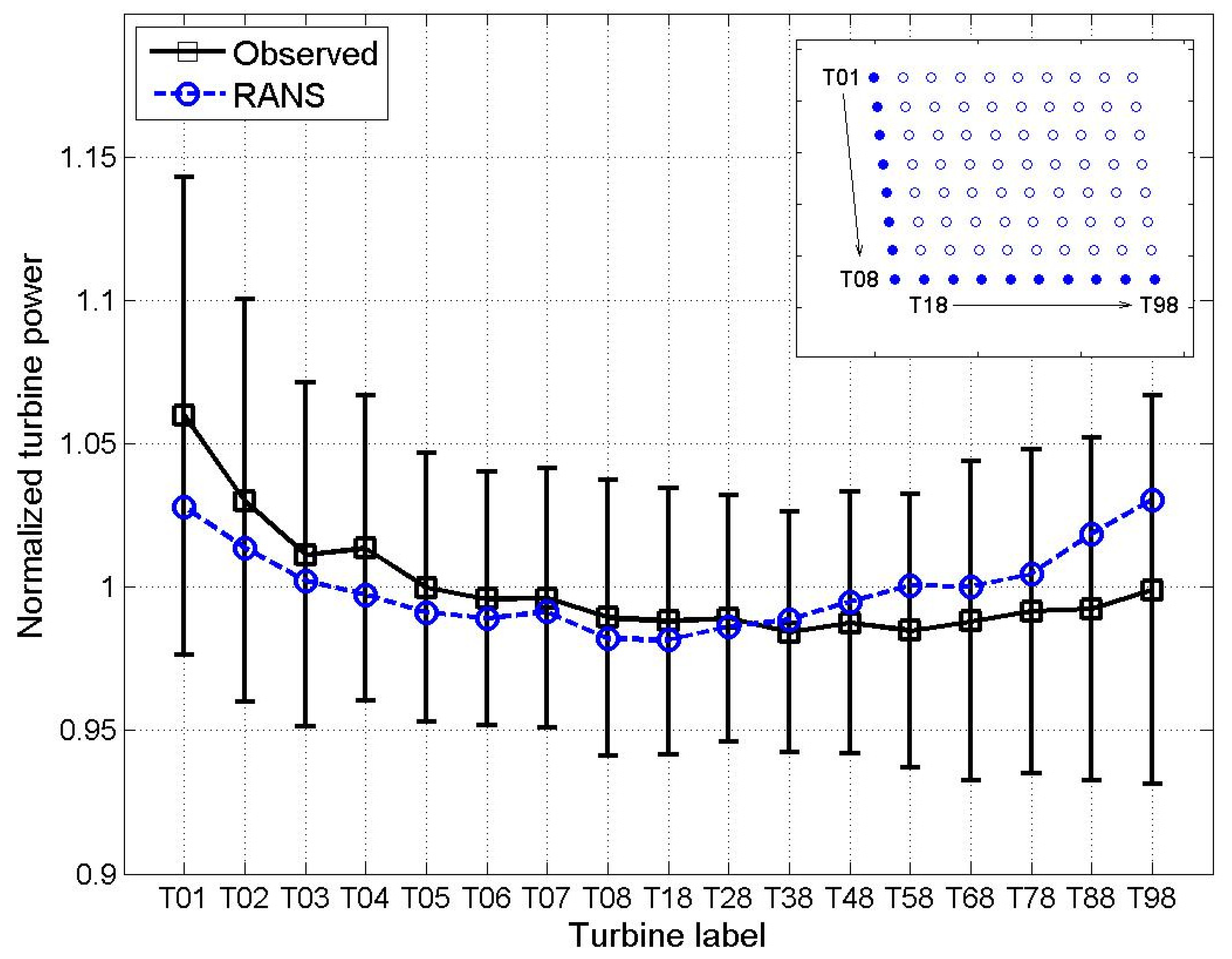
Before applying this model to the three onshore wind farms in this study, we ran a suite of verification and validation calculations focused on wind farm flows; included among these were simulations of the Horns Rev 1 wind farm. Model predictions of the row-by-row production variation at Horns Rev agree reasonably well with observations as shown in Figure 3. The measured results are sensitive to the details of the data filtering, so even though the RANS-predicted normalized powers are consistently 1–3% below the mean observed values, the gap closes considerably when comparing with the observations reported in [28] and reverses when comparing with the observations reported in [2].
We also compared results from the RANS model with observations of the production variation along the unwaked edges of Horns Rev 1 (Figure 4). The turbines at the far corners of the upstream perimeter produce more than those in the middle of the string, according to both observations and the RANS predictions. Unlike the predicted results, however, the observed production pattern has a pronounced skew, with turbines on the northwest end of the string producing more than those on the southeast end. The authors of [19,20] attributed the skew to the Coriolis effect and the related Ekman Spiral. Both effects are included in the RANS model, though the Ekman Spiral prescribed at the inlet of the domain may understate the actual mean direction variation with height at Horns Rev 1 for southwest flows (the modeled wind direction shifts +1.6° from the bottom of the rotor swept area to the top). Looking past the skew, the overall magnitude of the predicted production variation along this string of turbines is generally consistent with the observations.
Blockage effects arise from the two-way interaction that occurs between wind farm and atmosphere—we selected the modeling approach for this investigation accordingly. Of course, the RANS model does not directly simulate all aspects of this interaction. For example, the model bypasses details of the complex interplay between atmospheric turbulence and each three-bladed turbine, representing them instead with two-equation turbulence modeling, actuator disks, and one-dimensional turbine performance curves. The omitted details can have a significant impact on the near wake (within 2D downstream of the turbine), as well as on energy production over short time periods or within narrow wind direction sectors. These details appear to be less important, however, when it comes to predicting the far wake [29] or production over longer temporal and wider directional scales [28]. Their importance to this investigation may be even smaller. Not only do the results correspond to long time periods and wide direction ranges, but they also focus on blockage effects, which are far less turbulence-affected than wakes. Moreover, validation presented herein corroborates the model as a useful full-field complement to the point observations in this study.
The RANS simulations run at the three onshore wind farms targeted wind speeds and directions consistent with the filters used in the measured data analysis. Thus, the simulated turbines generally operated on the plateaus of their respective Ct curves, where a turbine’s influence on wind speeds upstream will be at a maximum.
To further mimic the data analysis, we ran two sets of simulations at each wind farm: one set with actuator disks to represent conditions after COD (wind farm simulations) and one without to represent conditions before COD (freestream simulations). The wind farm and freestream simulations share identical boundary conditions and meshes, so differences between the two sets of predicted flow fields are due to the presence of the modeled turbines alone. Each wind farm is small relative to the simulation domain, with the lateral and top boundaries at least 15 km from any turbine, thus mitigating the risk of any artificially induced blockage effects.
We also selected a few turbines at each wind farm to simulate in isolation. Combining the isolated-turbine and freestream results, we can accurately estimate for each simulated condition the power production of any wind farm turbine were it to be simulated in isolation. We can then quantify how the wind farm changes the energy production of each of its turbines relative to solitary operation.
4. Results
This section presents field observations and RANS simulations for three onshore wind farms. When depicting each wind farm, we rotate the coordinate system to obscure the project’s identity. The wind directions discussed herein are relative to these adjusted coordinate systems. In all three cases, we filtered the measured data to a 30° sector centered on 0°. The simulations ran in 10° wind direction increments, and from the resulting set of solutions we derived averaged quantities for the 30° sector.
Wind-farm-induced mean wind speed changes, as predicted by RANS, have much sharper spatial gradients downstream of the front row turbines than upstream. In turn, predictions at points upstream of the front row are much less sensitive to wind direction as compared to points downstream. Simulating in 10° direction increments, consequently, is more than sufficient to evaluate upstream wind speed changes in this study. In fact, throwing out every other simulation, leaving just a 20° increment, has a negligible impact on the results reported herein. Further, when computing the integrated average of the RANS results over a 30° sector, there is no need for additional weighting to account for wind direction uncertainty. Gaumond [28] showed how the use of additional weighting significantly improved predictions of waked turbine production over 5° wind direction sectors, but the weighting had virtually no effect on the results for a 30° sector—the same is true in this study.
4.1. Wind Farm A
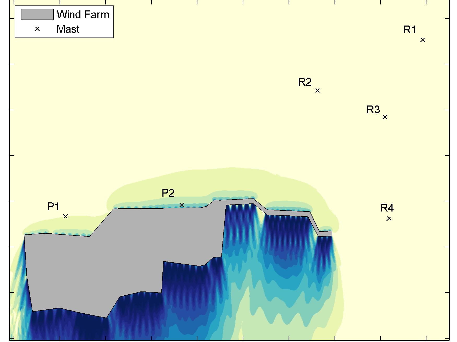
Wind Farm A has 87 turbines organized into east-west rows. The average hub-to-hub distance between neighboring turbines within a row is 3.2 D. The average distance between rows is 20 D. The terrain is simple with turbine base elevations all within 20 m of each other. The land cover consists of short grass, which the model represents with an aerodynamic roughness length () of 0.01 m. Figure 5 depicts the outline of the turbine layout as well as the locations of six masts. Masts P1 and P2 are respectively 10 D and 2 D upstream of the nearest turbine; they are considered perimeter masts in this analysis. The other four masts are much farther away and are considered reference masts. All of the masts have been recording wind data concurrently for just over a year before COD and after COD—with the exception of Mast R2, which only has 8 months of after-COD data.
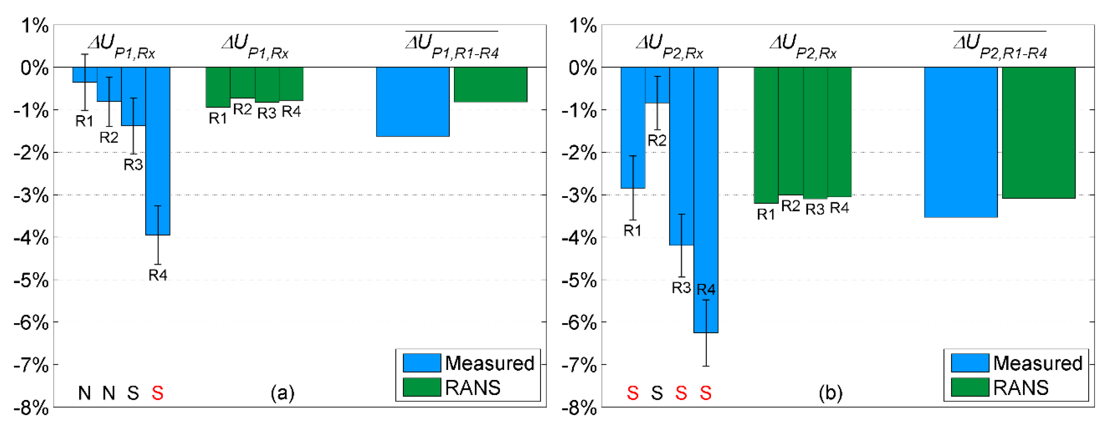
For each of the perimeter-reference mast pairs, both the measurements and RANS results indicate that the perimeter mast wind speeds slow relative to the reference mast wind speeds after the turbines are turned on. As shown in Figure 6, the observed slowdowns at the perimeter masts are sensitive to the choice of reference mast. This sensitivity suggests that additional factors, other than the wind farm, may be influencing measured for individual mast pairs. RANS predicts the impact of the wind farm on the reference mast wind speeds to be small (−0.16% to −0.36% relative to freestream), and thus the predictions vary little with reference mast. On average, RANS underpredicts the observed slowdowns at P1 and P2, but captures the trend between the two masts reasonably well.
The measurement heights above ground level varied from mast to mast in the Wind Farm A analysis: the P2 and R1 measurements were at hub height (H); the rest were at a height of 0.7 H (these masts did not have hub-height sensors). With the exception of Mast R2, the before-COD and after-COD time series are each a year long, reducing the risk of seasonal shear variations affecting the results. Nevertheless, we repeated the data analysis for measurements taken at a common set of heights, i.e., 0.7 H. As expected, the results changed little: decreased slightly to −1.8% and increased a bit to −3.3%. changed by just −0.2%. There was only 4 months of before-COD data for the 0.7 H sensor at Mast P2; this is one of the reasons why we used the hub-height sensors at P2 and R1 for the main analysis.
To further investigate the shorter after-COD time series at Mast R2, we also reran the data analysis using the same range of dates for the before and after time series, offset by one year. The impact of this change across all mast pairs, including those involving Mast R2, was minimal. Therefore, it does not appear as if the shorter after-COD time series at Mast R2 significantly affects the results.
Wind-farm-scale blockage is evident in all the RANS simulations. As can be seen in Figure 5, blockage slows approaching flow over a large area upstream of Wind Farm A; this effect is the result of two-way coupling between the wind turbine array and the atmosphere. A local, turbine-scale blockage effect, more commonly referred to as turbine induction, also contributes to the upstream slowdown, though the impact is largely limited to within a few rotor diameters of each turbine. Thus, while turbine-scale blockage from any individual turbine has little impact on wind speed at Mast P1, its impact on Mast P2 is not insignificant, according to the RANS results. When simulated in isolation, the turbine closest to Mast P2 decreases the predicted P2 wind speed by 1.2% relative to freestream for the sector of interest. When simulating the full wind farm, the predicted wind speed decrease at Mast P2 relative to freestream is 3.4%. Thus, the simulations suggest that wind-farm-scale blockage is the primary contributor to the observed slowdowns at Masts P1 and P2.
4.2. Wind Farm B
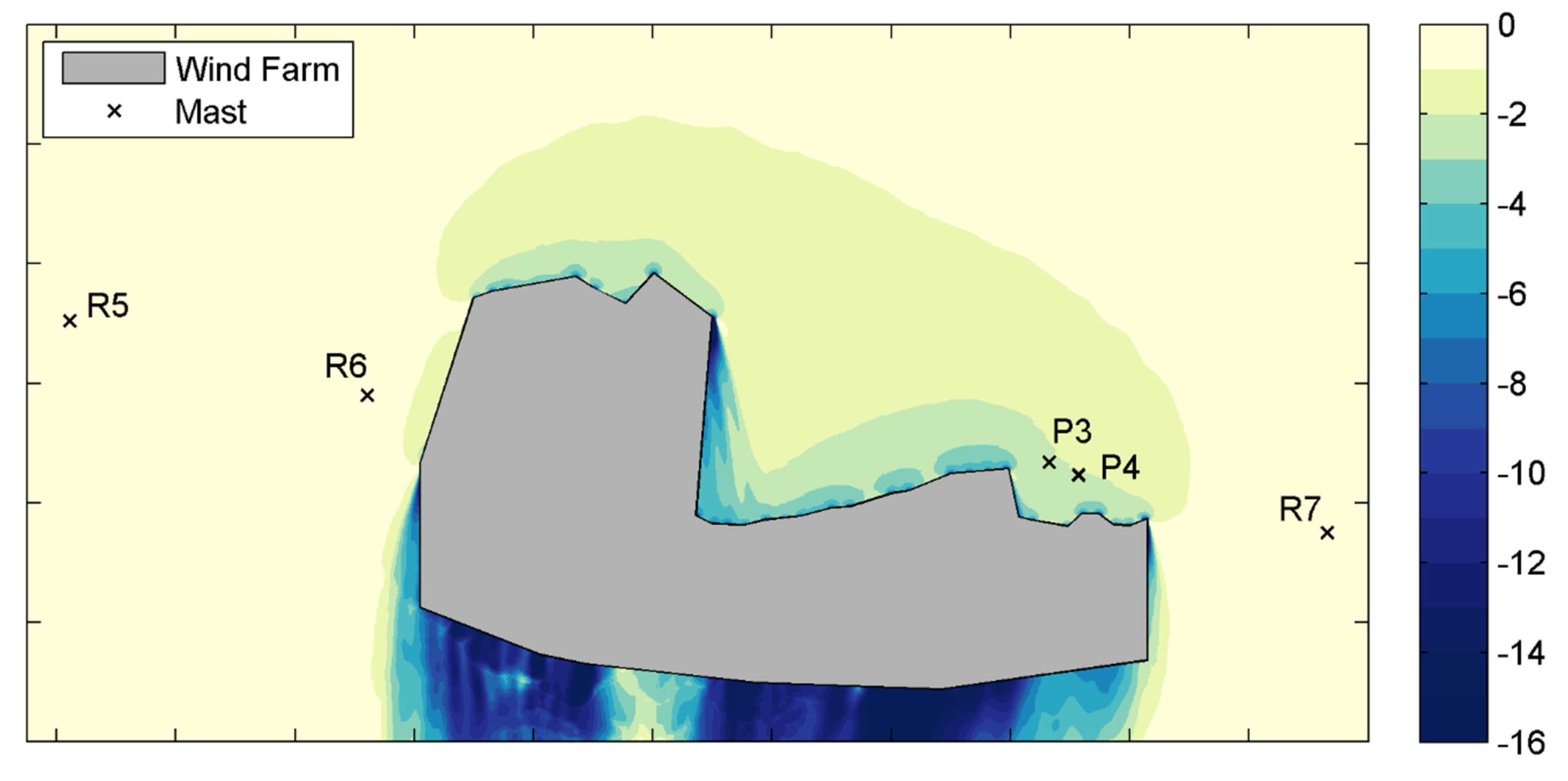
Wind Farm B has more than 80 turbines roughly organized into east-west rows. The average hub-to-hub distance between neighboring turbines is 3 D. Between the rows the average distance is 10 D. The terrain is moderately complex with turbine base elevations varying over a 90 m range and terrain slopes mostly between 0 and 4 degrees. The land cover on site is a mix of cropland and short shrubs, which we represent in the simulations with roughness lengths of 0.05 m and 0.1 m. Figure 7 depicts the outline of the turbine layout as well as the locations of five masts.
Masts P3 and P4 are respectively 10 D and 7 D from the nearest turbine downstream; they are considered perimeter masts in this analysis. The other three masts are farther away and more lateral to the wind farm; these masts are reference masts. All of the masts took hub-height wind measurements concurrently for more than a year before COD and after COD.
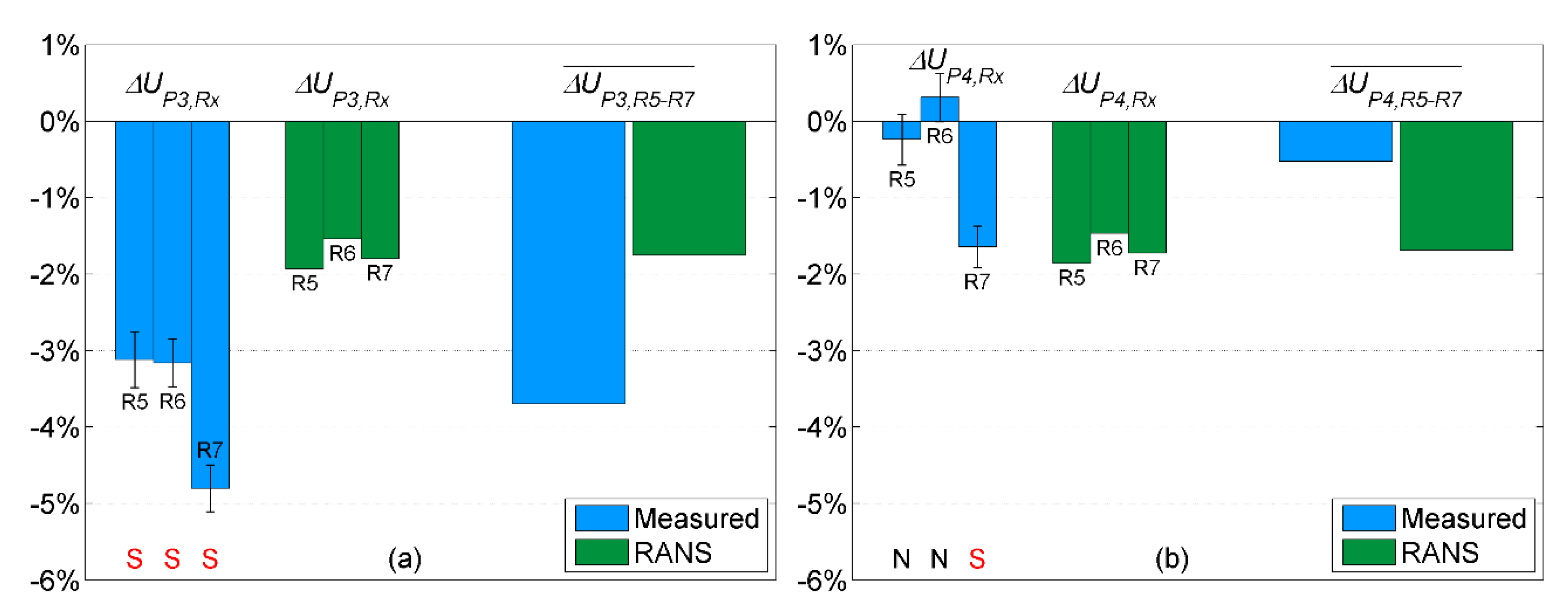
For five of the six perimeter-reference mast pairs, the measured perimeter mast wind speeds decrease relative to the reference mast wind speeds after the turbines are turned on (see Figure 8). RANS predicts such slowdowns for all six mast pairs. The observed slowdowns at the perimeter masts are sensitive to the choice of reference mast. As at Wind Farm A, we suspect that factors other than the wind farm contribute to this sensitivity. RANS predicts the reference mast wind speeds to change just a few tenths of a percent relative to freestream after COD (−0.21% for R5, −0.61% for R6, and −0.35% for R7), and thus the predictions are less sensitive to the choice of reference mast.
The average measured is a lot more negative for Mast P3 (Figure 8a) as compared to Mast P4 (Figure 8b)—despite P3 being farther from the wind farm and only 5 D away from P4. RANS predicts, on average, a much smaller difference between the two perimeter masts, with = −1.8% and = −1.7%. If we average over both the perimeter masts, the predicted wind speed change is closer to the observed change (−1.7% vs. −2.1%, respectively).
Wind-farm-scale blockage is evident in all the RANS simulations. The color contours in Figure 7 depict how, on average, blockage effectively slows approaching flow from the north. Single-turbine simulations indicate that induction from any individual turbine has a negligible impact on the wind speeds at P3 and P4. However, taken together the turbines create a wind-farm-scale blockage that appears to extend far upstream of the wind farm and is responsible for the observed slowdowns at the perimeter masts.
4.3. Wind Farm C
Wind Farm C has 100 turbines roughly organized into east-west rows. The average hub-to-hub distance between neighboring turbines is 3 D. The average distance between rows is 13 D. The terrain is simple with turbine base elevations all within 21 m of each other, and the land cover comprises short grass ( = 0.01 m). Figure 9 depicts the outline of the turbine layout along with the locations of three masts. Masts P5 and P6 are each just 2 D away from the nearest turbine downstream; they are considered perimeter masts in this analysis. Mast R8 is 11 D from the nearest turbine and is considered a reference mast.
The period of concurrent data for these masts is notably smaller than what we have at the other two wind farms. Before COD there are 6 months of concurrent data; after COD there are 5 months. All the measurements used in the analysis were taken at approximately the same height above ground (0.7 H), thus mitigating the potential impact of seasonal shear variation on the results. In addition, the ground is extremely flat in the area around and between the masts, which reduces the risk of meteorological differences between the two time series affecting the results.
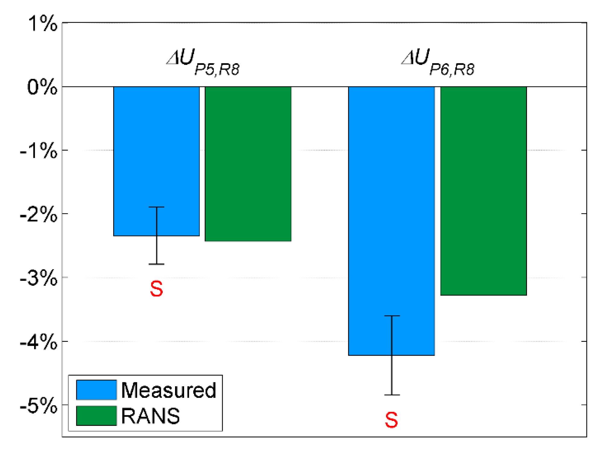
Measured and predicted wind speeds at Mast P5 and Mast P6 decrease relative to Mast R8 wind speeds after the turbines are turned on (see Figure 10). According to the RANS results, the wind farm also causes R8 wind speeds to decrease—by 1.3%. The distance between Mast R8 and the wind farm (11 D upstream) is similar to that of P1 at Wind Farm A (10 D upstream) and P3 at Wind Farm B (10 D upstream), locations where observations and RANS results indicate significant after-COD slowdowns relative to the reference masts. Thus, if Mast R8 were farther from Wind Farm C, the measured values would likely be even more negative than what we see in Figure 10.
Once again, wind-farm-scale blockage is evident in all RANS simulations. In Figure 9, blockage can be seen slowing flow as it approaches Wind Farm C from the north. According to single-turbine simulations, induction from the turbine closest to each perimeter mast decreases the wind speed by 1.2% at Mast P5 and 1.5% at Mast P6 compared to freestream conditions. When simulating the full wind farm, the predicted P5 and P6 after-COD slowdowns relative to freestream are 3.7% and 4.5%, respectively. Thus, the simulations indicate that both turbine-scale and wind-farm-scale blockage contribute to the observed slowdowns at P5 and P6, with wind-farm-scale blockage making the larger contribution.
Across all the perimeter-reference pairs in this study, the average measured for perimeter masts 2 D upstream of a wind farm is −3.4%; for the perimeter masts 7–10 D upstream, the average measured is −1.9%. By comparison, the RANS-predicted values are −3.0% and −1.4%, respectively. If we instead bin the mast pairs by wind farm, the average predicted values are also reasonably consistent with, though somewhat less pronounced than, the averaged measured values: −2.6% measured vs. −2.0% predicted at Wind Farm A; −2.1% vs. −1.7% at B; and −3.3% vs. −2.9% at C.
Factors other than the wind farm could potentially influence measured . Measurement inconsistency is a possible influence. If, for example, a wind speed sensor degraded during the after-COD period, it would affect the related values. We mitigate this risk using EPA best practices for checking and cleaning measured data.
Sampling error could also contribute to differences between the means of the before and after data. This possibility adds uncertainty to the measured values for individual mast pairs, though the level of uncertainty is generally less than the signal we are measuring. A one-tailed Mann-Whitney analysis shows that 12 of the 16 mast pairs have a p-value below 0.05, indicating that the corresponding values reflect a statistically significant after-COD change to the perimeter-reference wind speed relationship. The four p-values above 0.05 correspond to values close to 0%, including the one mast pair with a positive . We cannot statistically rule out the possibility that the perimeter-reference wind speed relationship stays the same after COD for these four mast pairs. Of the 12 statistically significant results, 10 of them had p-values below 2 × 10⁻⁶, indicating extremely high confidence that the perimeter-reference wind speed relationship changed after COD—this set of 10 mast pairs includes all six of the perimeter masts in this study. Thus, the statistical analysis, in conjunction with the consistently negative values, offers strong evidence that during the measurement periods the wind speeds at the perimeter masts decrease relative to wind speeds farther away after the turbines are turned on.
Meteorological differences between the before and after data periods are another potential influence on . The wind speed relationship between two mast locations can be sensitive to the background meteorological conditions—to stable vs. unstable flows, for example [24]. Thus, if the overlying meteorology is significantly different between the before-COD and after-COD periods, it could cause to deviate from 0.0%, even if the turbines are never turned on. Using multiple reference masts in varied locations can help mitigate this risk—as can using long before and after time series. We do both in this study. Of the 16 mast pairs, 12 have one year of concurrent wind speed measurements before COD as well as after COD. For the reasons discussed earlier in this section, the shorter time series at the other four mast pairs are unlikely to make the corresponding results significantly more vulnerable to before vs. after meteorological differences.
To better understand the remaining risk of non-wind-farm-related factors affecting , we conducted an additional analysis designed to further mitigate unsought influences. In this analysis, instead of , we calculate , replacing the reference mast data with semi-synthetic data at the perimeter mast. The before-COD PssR data are real perimeter mast measurements; the after-COD PssR wind speed data are synthetic, meaning the records derive from measurements taken at other places and times. In this case, we scale the after-COD reference mast data using linear coefficients derived from before-COD data binned by wind direction and time of day—with daytime and night-time used roughly to differentiate unstable vs. stable surface conditions (at these inland sites, which are far from any large bodies of water, daytime records mostly correspond to unstable surface conditions, and night-time records mostly correspond to stable surface conditions). The new synthetic wind speed data represent a rough estimate of what the perimeter mast data would be if the wind farm was not built. The values derived from these data are more negative on average than the values (−3.3% vs. −2.5%, respectively), and once again, 15 out of the 16 values are negative ( is the outlier). Of course, using synthetic data carries its own set of uncertainties, and we cannot reasonably claim that the approach fully controls for unsought influences. Nevertheless, the results are reasonably consistent with and do not uncover any red flags in the primary data analysis.
Notwithstanding all the mitigating steps and extra analysis, we cannot rule out that some of these factors (statistical uncertainty, measurement inconsistency, year over year meteorological differences) could still potentially affect the result for an individual mast pair. We actually suspect that they do—given, for example, the sensitivity of the results to reference mast in Figure 6. These factors, however, are very unlikely to produce a persistent negative bias across multiple wind farms and a large set of mast pairs. Measured is negative for 15 of the 16 mast pairs (20 of 21 if we include the additional measurement heights at Wind Farm A). We have no reason to believe any of these factors could so consistently reduce perimeter mast wind speeds relative to reference mast wind speeds, after the wind farms begin operation. We do, however, have reason to believe that the wind farms could cause such consistently observed slowdowns. Separate wind tunnel and LES studies have shown such an effect [12,13,14], and the RANS results herein, which absolutely isolate wind farm impact, include upstream slowdowns that are reasonably consistent with average measured , whether binned by distance upstream or by wind farm. We therefore conclude that the presence of the wind farms is very likely the primary cause behind the significant wind speed reductions observed at the perimeter masts after COD. We are not aware of any other plausible explanation for the results.
5. Implications
These findings have several implications, which build upon each other towards the main conclusion of this paper: Widely used procedures for estimating wind farm energy production likely contain significant overprediction bias. We briefly list the implications here and then follow with the details and reasoning behind each:
- Wind speeds at upstream perimeter masts are lower than freestream
- Lower mast wind speeds mean the individual turbines just downstream produce less energy than current EPA practices would estimate
- The group of turbines on the upstream perimeter of a wind farm also produce less than EPA practices would estimate
- Prediction bias on the upstream perimeter pervades the wind farm
- The magnitude of the overprediction bias in the wakes-only approach to turbine interaction can be significant
- Power curves are probably an additional source of bias
5.1. Perimeter Mast Wind Speeds Are Lower than Freestream
The measurements show that wind speeds near the upstream perimeter of a wind farm decrease relative to locations farther away after the turbines are turned on. Understanding how these wind speeds change relative to freestream conditions requires additional considerations. It is very unlikely that the wind farm causes perimeter mast wind speeds to increase relative to freestream. To be consistent with observations, this would mean larger increases at the reference masts and imply that the wind farm’s influence intensifies with distance from the wind farm—an implausible set of circumstances. Much more likely, the wind farm causes wind speeds at the perimeter masts to decrease relative to freestream conditions. This conclusion has a credible physical explanation (i.e., blockage effects) and is consistent with the RANS results, which predict near-perimeter slowdowns relative to freestream well in excess of what can be attributed to individual turbine induction.
5.2. Lower Mast Wind Speeds Mean Nearby Turbines Will Underproduce Compared to Expectations
If one were to place a wind turbine at any of the perimeter mast locations, it would produce less than it would if the wind farm downstream was not present. The observed and predicted slowdowns also have implications for the energy production of the wind farm itself. The slowdowns induced 7–10 D upstream of the wind farms (masts P1, P3, and P4) imply that the turbines downstream of the front row of a wind farm may have a similar impact on wind conditions at the front row—as the distance between these two sets of turbines is often around 7–10 D. This would cause the front row turbines to produce less than they would if the turbines downstream were not there. We can draw stronger conclusions from slowdowns observed closer to the wind farms.
Single-turbine RANS simulations run back-to-back with full wind farm simulations (same wind conditions, domain, and mesh) indicate that the turbines a few rotor diameters downstream of masts P2, P5, and P6 will produce less energy than they would operating in isolation. It is not possible to confirm this finding with a similar experiment in the field; however, the presented observations are sufficient to conclude that current EPA practices will overestimate the production of these turbines. We know this because of the way that turbine power performance is measured. The measurement campaign typically involves a turbine on the perimeter of a wind farm and a hub-height mast 2–4 D upstream of the turbine in the prevailing wind direction [30]. Wind speed and power measurements are taken concurrently and processed to create a power curve, with turbine power a tabular function of wind speed. The wind industry has obtained measured power curves from the perimeters of hundreds of wind farms, including Wind Farms A and C where masts P2, P5, and P6 supplied wind speed data to power performance tests (PPTs).
When estimating the energy production of an unwaked turbine, a typical EPA will take the freestream wind resource (i.e., the horizontal wind speed distribution at hub height absent the presence of the wind farm) and apply it to the turbine power curve. If we were to follow the same approach and apply the P2 freestream resource for northerly flows to the tested turbine’s measured power curve, we would likely overestimate the energy production—because, as we have shown, Mast P2 wind speeds are lower than freestream for northerly flows when the wind farm is operating. Studies indicate that power curves used in EPAs are on average generally consistent with, and no less energetic than, measured curves [31,32,33,34,35]. Thus, slowdowns evident 2–4 D upstream of a wind farm translate to an overprediction bias in the energy estimate for nearby turbines.
5.3. The Group of Turbines on the Upstream Perimeter Will Underproduce Compared to Expectations
These wind-farm-induced slowdowns are not limited to the perimeter masts, nor is the associated overprediction bias limited discontinuously to one or two nearby turbines. The observed production pattern at Horns Rev 1 reveals a coherent and generally continuous variation in energy production along the upstream edges of the project (Figure 4), a pattern consistent with observations at many other wind farms [21]. RANS simulations indicate that wind-farm-scale blockage diverts flow away from the central turbines on the upstream edge(s) of a wind farm. Some of this flow travels laterally towards turbines closer to the sides of the wind farm, accounting for at least some of the observed production variation. The rest of the diverted flow, however, passes over and around the simulated wind farm, resulting in a net production loss ([36] and [37] contain observational trends consistent with this finding). In fact, the RANS results indicate that nearly every turbine along the upstream rows of Wind Farms A–C and Horns Rev 1 produces less energy than it would in isolation. The wakes-only approach, in contrast, assumes that front row turbines, collectively and individually, produce the same amount of energy as they would operating in isolation. Therefore, current EPA practices overestimate energy production for the group of turbines on the upstream perimeter of a wind farm.
5.4. Prediction Bias on the Upstream Perimeter Pervades the Wind Farm
Because of the way turbine interaction models are designed and validated, prediction bias for upstream perimeter turbines extends to the entire wind farm. The wind energy community validates these models against, and tunes them to, observations like those presented in Figure 3, where energy production is normalized by an upstream perimeter row or turbine. Validation across many wind farms indicate that, on average, the most commonly used models predict the row-by-row production variation with reasonable accuracy and, critical to this discussion, without bias relative to the upstream row [2,5,38]. Thus, if wind-farm-scale blockage causes an upstream row of turbines to underproduce isolated operation by 1%, then EPA approaches that ignore blockage—that is, nearly all of them—will on average overpredict energy production for the entire wind farm by the same 1%.
5.5. The Wakes-Only Prediction Bias Can Be Large
The RANS results indicate this bias can be much greater than 1%. To estimate the bias, we adjust the RANS-predicted power at each wind farm turbine to represent the power that would be predicted using the wakes-only approach. The adjustments increase predicted wind farm power production, but maintain the pattern of production in such a way that, for example, the predicted row-by-row variation in Figure 3 would stay the same. The details of the adjustment procedure are as follows:
- For each unwaked turbine, replace the RANS-predicted turbine power from the wind farm simulation () with the turbine power corresponding to its simulation in isolation ().
- Calculate a scaling factor equal to the factor by which Step 1 increases the total predicted power of the unwaked, waking turbines. Unwaked, non-waking turbines, such as those on the eastern end of Wind Farm A (Figure 5), are not included in the calculation of this factor.
- For each waked turbine, apply the scaling factor to the RANS-predicted power, , in order to preserve the original power relationship between the waked turbines and the unwaked turbines waking them.
The outcome of this procedure is a new set of power values, , representing an estimate of what a wakes-only-type model would predict for each wind farm turbine. We can then calculate the wakes-only prediction bias using the following formula:
where is the sum of the RANS-predicted power for each wind farm turbine, and is the sum of the turbine powers converted to represent wakes-only predictions. Using similar concepts, we can also calculate the neglected loss as a fraction of ideal power generation and compare with the total turbine interaction loss, :
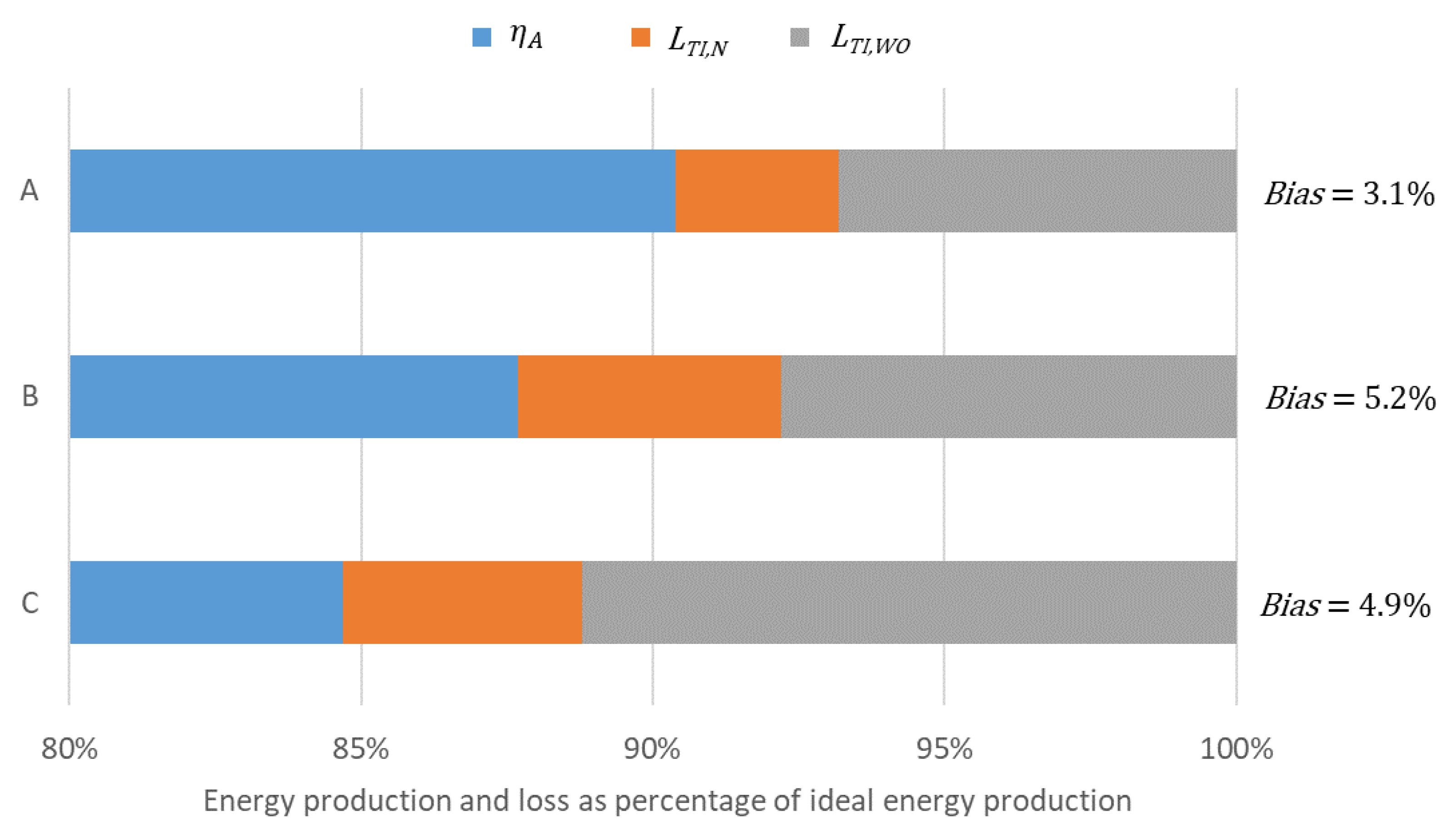
where is ideal power generation for the wind farm (i.e., the sum of each turbine producing as if operating in isolation). is the wind farm turbine interaction loss as would be calculated using a wakes-only model, and is the portion of the turbine interaction loss neglected by such a model. The array efficiency, , is 1 − .
Although related to the neglect of blockage effects, should not be confused with blockage loss. In general, it is difficult, if not impossible, to precisely divide the energy reduction due to turbine interaction into blockage loss and wake loss. Both wakes and blockage change the wind speed at the rotor face of an interior turbine and parsing their respective impacts is not straightforward. Even a well-validated wakes-only model cannot reliably isolate the wake loss. This is because, as indicated above, wakes-only models are tuned and validated to accurately predict the row-by-row variation of power production, and since part of the observed variation is due to row-by-row variation in the blockage loss, wakes-only flow models indirectly account for some of the impact of blockage. Of course, these models still completely neglect the impact of blockage on front row turbines and thereby underestimate the overall power production level.
Figure 11 summarizes the RANS-predicted turbine interaction losses at the three onshore wind farms while highlighting the portion neglected by the wakes-only approach; it also reports the related energy production prediction bias. The blue bars ( represent the RANS-predicted array efficiency; blue plus red (, or ) is the array efficiency as would be predicted by a wakes-only model.
According to the RANS results, the wakes-only approach can neglect a significant fraction of the turbine interaction loss, resulting in a substantial energy prediction bias. That said, the loss and bias levels shown in Figure 11 correspond to the simulated conditions only. The simulated wind speeds generally put each turbine on the plateau of the Ct curve and below the knee of the power curve, where the impact of blockage on wind speed is at a high and power is most sensitive to wind speed. Bias related to blockage will be lower at higher wind speeds; it will also likely vary with wind direction. Wake losses are similarly sensitive to wind speed, but integrated over all conditions, they have a material impact on the production of most wind farms and must be accounted for in EPAs—as they routinely are. Likewise, extra-wake turbine interaction probably impacts overall energy production to a material degree at many wind farms, if not most of them, and therefore, these effects must also be accounted for.
5.6. Bias in Power Curves
For a given freestream wind resource, accurate prediction of a turbine’s energy production requires: (1) a power curve that faithfully represents the turbine’s production when operating in isolation and (2) an accurate estimate of how that production changes when the other wind farm turbines are present. This paper focuses on the second requirement; however, blockage may also represent a bias in the first. Power curves used in EPAs are invariably assumed to be functions of freestream wind speed, but to the extent that these curves are influenced by and are consistent with PPT curves, this assumption is very likely false. The results from Wind Farms A and C, as well as lidar measurements from eight offshore wind farms reported in [39], clearly show that the wind speeds at a PPT mast are lower than freestream. The measured curves should be corrected to account for the impact of local blockage from the tested turbine on the PPT mast, as well as for any influence of the wind farm on the wind speed relationship between the PPT mast and the rotor face. The objective is a curve that can accurately predict the production of an isolated turbine operating in a known set of freestream conditions. The power curves currently used in EPAs will likely on average overpredict this production, as these curves are clearly connected to measured curves [31,32,33,34,35], which currently do not include the above-recommended corrections [30].
6. Conclusions
Field observations at three wind farms reveal significant wind speed reductions upstream of each project. The primary cause behind these reductions is very likely the presence of the wind farms themselves. Correspondingly, RANS solutions, which are in reasonable agreement with measurements, consistently exhibit wind-farm-scale and turbine-scale blockage slowing upstream flow as it approaches each wind farm. The magnitude and spatial reach of the measured and simulated slowdowns call into question widely used assumptions regarding the upstream influence of wind turbines. These findings, in turn, indicate that energy assessment procedures used throughout the wind energy community likely contain a material overprediction bias.
The results point to two sources of bias: power curves and turbine interaction models. This paper focuses on bias in the wakes-only approach to turbine interaction, which assumes that the turbines on the upstream row of a wind farm produce energy as if each one is operating in isolation. In actuality, these turbines, as a group, very likely underproduce isolated operation—and the related prediction bias extends to the entire wind farm. An analysis of numerical simulation results indicates that the wakes-only approach can neglect a substantial fraction of the total turbine interaction loss—over a quarter of the loss in the cases presented herein. As a result, wakes-only-type models will generally overpredict wind farm energy production.
Wind-farm-scale blockage is at the root of this bias. Compared with wakes, these blockage effects, and the gradual wind speed changes associated with them, resist direct observation. Nevertheless, a growing collection of evidence—wind tunnel measurements, patterns of turbine production, and now the results herein—points to the pronounced influence of these effects.
When new findings challenge the status quo, the strength of evidence behind the existing approach must be considered before making a change. In the case of the wakes-only approach to turbine interaction, we do not have supporting evidence. Some may yet be found: There remain large gaps in the available empirical record, and as future studies fill these gaps, the suitability of the wakes-only approach will no doubt become more clear. In the meantime, however, the balance between the evidence contravening this approach (strong) and the evidence supporting it (weak, if any) is now so one-sided that its continued use is difficult to justify. The wakes-only approach likely neglects important influences on wind farm energy production and should be replaced. A switch to a more complete approach—supported with well-validated prediction methods—will reduce bias and uncertainty in energy production assessments and likely lead to more efficient wind farm designs.
Author Contributions
Conceptualization, J.B.; Data curation, M.P., R.R. and E.T.; Formal analysis, J.B., M.P., R.R. and E.T.; Investigation, J.B., M.P., R.R. and E.T.; Methodology, J.B.; Project administration, J.B.; Software, J.B. and R.R.; Supervision, J.B.; Validation, J.B., M.P., R.R. and E.T.; Visualization, J.B.; Writing-original draft, J.B.; Writing-review & editing, J.B.
Funding
This research was funded by Innovate UK, Project 102239.
Acknowledgments
Additional funding came from DNV GL. Field observations were provided by EDF Energy Renewables and Ørsted. We also wish to thank and acknowledge the many individuals who assisted with this work: Stefanie Bourne, Jean-François Corbett, Marie-Ann Cowen, Dnyanesh Digraskar, Melissa Elkinton, Taylor Geer, Trenton Gilbert, Paul Housley, Heather Hurree, Cory Jog, Lars Landberg, Christiane Montavon, Nicolai Gayle Nygaard, Jack Orrell, Carl Ostridge, Christian Peake, Chris Rodaway, and Jon Woodcock.
Conflicts of Interest
The authors declare no conflict of interest.
References
- Sanderse, B. Aerodynamics of Wind Turbine Wakes—Literature Review; Report ECN-E-09-016; Energy Research Center of the Netherlands: Petten, The Netherlands, 2009. [Google Scholar]
- Walker, K.; Adams, N.; Gribben, B.; Gellatly, B.; Nygaard, N.G.; Henderson, A.; Jiménez, M.M.; Schmidt, S.R.; Ruiz, J.R.; Paredes, D.; et al. An evaluation of the predictive accuracy of wake effects models for offshore wind farms. Wind Energy 2015. [Google Scholar] [CrossRef]
- Frandsen, S.; Barthelmie, R.; Pryor, S.; Rathmann, O.; Larsen, S.; Højstrup, J. Analytical modelling of wind speed deficit in large offshore wind farms. Wind Energy 2006, 9, 39–53. [Google Scholar] [CrossRef]
- DNV GL. WindFarmer Theory Manual; Version 5.3; DNV GL: Bristol, UK, 2014; pp. 14–20. [Google Scholar]
- Brower, M.C.; Robinson, N.M. The OpenWind Deep-Array Wake Model; AWS Truepower: Albany, NY, USA, 2012. [Google Scholar]
- Rodrigo, J.S.; Moriarty, P.; Nouqueret, E.C.; Arroyo, R.A.C.; Churchfield, M.; Hansen, K.S. WAKEBENCH Best Practice Guidelines for Wind Farm Flow Models, 1st ed.; IEA-Wind Task 31; International Energy Agency: Paris, France, 2015. [Google Scholar]
- Clifton, A.; Smith, A.; Fields, M. Wind Plant Preconstruction Energy Estimates: Current Practice and Opportunities; Report NREL/TP-5000-64735; National Renewal Energy Laboratory: Golden, CO, USA, 2016. [Google Scholar]
- Manwell, J.F.; McGowan, J.G.; Rogers, A.L. Wind Energy Explained: Theory, Design and Application, 2nd ed.; Wiley: Hoboken, NJ, USA, 2010; pp. 423–427. [Google Scholar]
- Barthelmie, R.J.; Jensen, L.E. Evaluation of wind farm efficiency and wind turbine wakes at the Nysted offshore wind farm. Wind Energy 2010, 13, 573–586. [Google Scholar] [CrossRef]
- Farris, S.; Henderson, A.; Whiting, R.; Fields, J.; Sherwin, B. IEC 61400-15 Assessment of Wind Resource, Energy Yield and Site Suitability Input Conditions for Wind Power Plants; Offshore Wind Energy: London, UK, 2017. [Google Scholar]
- Barthelmie, R.J.; Hansen, K.; Fransen, S.; Rathmann, O.; Schepers, J.G.; Schlez, W.; Phillips, J.; Rados, K.; Zervos, A.; Politis, E.S.; et al. Modelling and measuring flow and wind turbine wakes in large wind farms offshore. Wind Energy 2009, 12, 431–444. [Google Scholar] [CrossRef]
- Ebenhoch, R.; Muro, B.; Dahlberg, J.A.; Hägglund, P.B.; Segalini, A. A linearized numerical model of wind-farm flows. Wind Energy 2016. [Google Scholar] [CrossRef]
- Allaerts, D.; Meyers, J. Gravity waves and wind-farm efficiency in neutral and stable conditions. Bound.-Layer Meteorol. 2017, 166, 269–299. [Google Scholar] [CrossRef]
- Wu, K.L.; Porté-Agel, F. Flow adjustment inside and around large finite-size wind farms. Energies 2017, 10. [Google Scholar] [CrossRef]
- Nishino, T.; Draper, S. Local blockage effect for wind turbines. J. Phys. Conf. Ser. 2015, 625. [Google Scholar] [CrossRef]
- Nishino, T.; Willden, R.H.J. The efficiency of an array of tidal turbines partially blocking a wide channel. J. Fluid Mech. 2012, 708, 596–606. [Google Scholar] [CrossRef]
- McTavish, S.; Rodrigue, S.; Feszty, D.; Nitzsche, F. An investigation of in-field blockage effects in closely spaced lateral wind farm configurations. Wind Energy 2015, 18, 1989–2011. [Google Scholar] [CrossRef]
- Forsting, A.R.M.; Troldborg, N.; Gaunaa, M. The flow upstream of a row of aligned wind turbine rotors and its effect on power production. Wind Energy 2017, 20, 63–77. [Google Scholar] [CrossRef]
- Mitraszewski, K.; Hansen, K.S.; Nygaard, N.G.; Rethoré, P.E. Wall Effects in Offshore Wind Farms. In Proceedings of the Torque Conference, Oldenburg, Germany, 9–11 October 2012. [Google Scholar]
- Seshadhri, S.; Montavon, C.; Jones, I. Coriolis Effects in the Simulation of Large Array Losses: Preliminary Results on ‘Wall Effect’ and Wake Asymmetry. In Proceedings of the EWEA Offshore, Copenhagen, Denmark, 4–7 February 2013. [Google Scholar]
- Jog, C.; (EDF Energy Renewables, Portland, OR, USA); Nygaard, N.G.; (Ørsted, Copenhagen, Denmark). Personal communications, 2017.
- Mann, H.B.; Whitney, D.R. On a test of whether one or two random variables is stochastically larger than the other. Ann. Math. Stat. 1947, 18, 50–60. [Google Scholar] [CrossRef]
- Siemens PLM Software. User Guide for STAR-CCM+; Version 12; Siemens PLM Software: Plano, TX, USA, 2017. [Google Scholar]
- Bleeg, J.; Digraskar, D.; Woodcock, J.; Corbett, J.F. Modeling stable thermal stratification and its impact on wind flow over topography. Wind Energy 2014. [Google Scholar] [CrossRef]
- Bleeg, J.; Digraskar, D.; Horn, U.; Corbett, J.F. Modelling Stability at Microscale, Both Within and Above the Atmospheric Boundary Layer, Substantially Improves Wind Speed Predictions. In Proceedings of the EWEA Conference, Paris, France, 17–20 November 2015. [Google Scholar]
- Thunis, P.; Bornstein, R. Hierarchy of Mesoscale Flow Assumptions and Equations. J. Atmos. Sci. 1995, 53, 380–397. [Google Scholar] [CrossRef]
- Van der Laan, M.; Sørensen, N.N.; Réthoré, P.E.; Mann, J.; Kelly, M.C. The k-ε-fp model applied to double wind turbine wakes using different actuator disk force methods. Wind Energy 2014. [Google Scholar] [CrossRef] [Green Version]
- Gaumond, M.; Réthoré, P.E.; Ott, S.; Peña, A.; Bechmann, A.; Hansen, K.S. Evaluation of the wind direction uncertainty and its impact on wake modeling at the Horns Rev offshore wind farm. Wind Energy 2014, 17, 1169–1178. [Google Scholar] [CrossRef] [Green Version]
- Troldborg, N.; Zahle, F.; Réthoré, P.E.; Sørensen, N.N. Comparison of wind turbine wake properties in non-sheared inflow predicted by different computational fluid dynamics rotor models. Wind Energy 2015, 18, 1239–1250. [Google Scholar] [CrossRef]
- International Electrotechnical Commission. IEC 61400-12-1:2017, Wind Energy Generation Systems–Part. 12-1: Power Performance Measurements of Electricity Producing Wind Turbines; International Electrotechnical Commission: Geneva, Switzerland, 2017. [Google Scholar]
- Brower, M. Wind Turbine Performance: Issues and Evidence. Presented at the EWEA Conference, Lyon, France, 2–3 July 2012. [Google Scholar]
- Harman, K. How Does the Real World Performance of Wind Turbines Compare with Sales Power Curves. Presented at the EWEA Conference, Lyon, France, 2–3 July 2012. [Google Scholar]
- Young, M. Power Curve Measurement Experiences and New Approaches. Presented at the EWEA Resource Assessment Workshop, Dublin, Ireland, 21 November 2013. [Google Scholar]
- Ostridge, O. Understand & Predicting Turbine Performance. Presented at the AWEA Wind Resource & Project Energy Assessment Seminar, Orlando, FL, USA, 2–3 December 2014. [Google Scholar]
- Bernadett, D. Power Curve Loss Adjustments at AWS Truepower. Presented at the 20th meeting of the Power Curve Working Group, Minneapolis, MN, USA, 29 September 2016. [Google Scholar]
- Nygaard, N.G.; Hansen, S.D. Wake effects between two neighbouring wind farms. J. Phys Conf. Ser. 2016, 625. [Google Scholar] [CrossRef]
- Hägglund, P.B. An Experimental Study on Global Turbine Array Effects in Large Wind Turbine Clusters. Master’s Thesis, KTH Royal Institute of Technology, Stockholm, Sweden, 2013. [Google Scholar]
- Geer, T. Improving Confidence in Wake Predictions through Operational Validations. Presented at Wind Europe Offshore, London, UK, 6–8 June 2017. [Google Scholar]
- Nygaard, N.G.; Brink, F.E. Measurements of the Wind Turbine Induction Zone. Presented at the Wind Energy Science Conference, Lyngby, Denmark, 26–29 June 2017. [Google Scholar]
Figure 1.
Top view schematic of three wind farm/turbine configurations: (a) multi-row wind farm; (b) single turbine row; and (c) isolated wind turbine. The symbol sizes represent rotor size. Arrows indicate the wind direction. A single wind turbine location, highlighted in bold, is in all three configurations.

Figure 2.
Schematic of a generic wind farm, with circles representing turbines and x-marks representing meteorological masts. Arrows indicate the prevailing wind direction.
Figure 2.
Schematic of a generic wind farm, with circles representing turbines and x-marks representing meteorological masts. Arrows indicate the prevailing wind direction.

Figure 3.
Row-by-row energy production at the Horns Rev 1 wind farm normalized by the energy production of the westernmost north-south row (Row 1). The values correspond to wind directions between 255° and 285° (westerly flow). The observations were filtered to a nominal freestream wind speed range of 7.5–8.5 m/s as inferred from the unwaked wind turbines. The RANS-simulations corresponded to a freestream wind speed of 8.3 m/s. The error bars represent standard deviations.
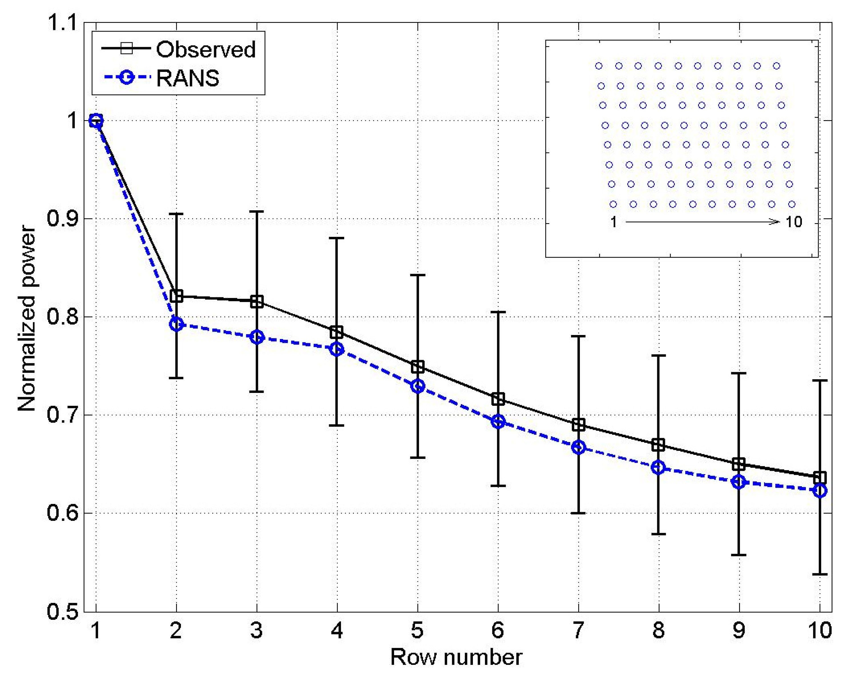
Figure 4.
Observed and RANS-predicted power production pattern at the Horns Rev 1 wind farm normalized by the mean of the distribution. The values correspond to the 10° wind direction sector centered on 208° (southwesterly flow). The observations were filtered to a nominal freestream wind speed range of 4–12.5 m/s as inferred from the unwaked wind turbines. The RANS-simulations corresponded to a freestream wind speed of 8.3 m/s. The error bars represent standard deviations.

Figure 5.
Wind Farm A and its influence on nearby flow at turbine hub height. The colors represent the predicted percent change in wind speed relative to freestream conditions for the 30° wind direction sector centered on 0° (northerly flow). Each color level corresponds to a range of 1.0%. The tick marks on the border of the plot correspond to a distance increment of 2 km.
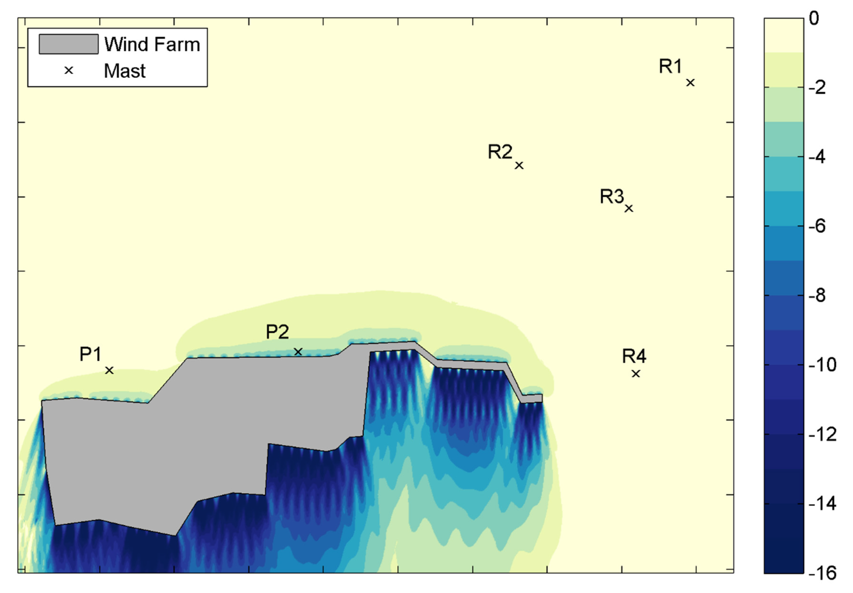
Figure 6.
Measured and predicted values at Wind Farm A. The left plot (a) shows results from Mast P1, and the right plot (b) shows results for Mast P2. The narrow bars on each plot correspond to individual perimeter-reference mast pairs. The wide bars are averages over the four reference masts. The “S” or “N” below each measured result denotes whether or not (S or N) reflects a statistically significant change in the wind speed relationship between masts Px and Rx. A red “S” denotes a p-value below 2 × 10⁻⁶. The black error bars represent the standard error of measured .

Figure 7.
Wind Farm B and its influence on nearby flow at turbine hub height. The colors represent the predicted percent change in wind speed relative to freestream conditions for the 30° wind direction sector centered on 0° (northerly flow). Each color level corresponds to a range of 1.0%. The tick marks on the border of the plot correspond to a distance increment of 2 km.

Figure 8.
Measured and predicted
values at Wind Farm B. The left plot (a) shows results from Mast P3, and the right plot (b) shows results for Mast P4. The narrow bars on each plot correspond to individual perimeter-reference mast pairs. The wide bars are averages over the three reference masts. The “S” or “N” below each measured result denotes whether or not (S or N) reflects a statistically significant change in the wind speed relationship between masts Px and Rx. A red “S” denotes a p-value below 2 × 10⁻⁶. The black error bars represent the standard error of measured .

Figure 9.
Wind Farm C and its influence on nearby flow at turbine hub height. The colors represent the predicted percent change in wind speed relative to freestream conditions for the 30° wind direction sector centered on 0° (northerly flow). Each color level corresponds to a range of 1.0%. The tick marks on the border of the plot correspond to a distance increment of 2 km.
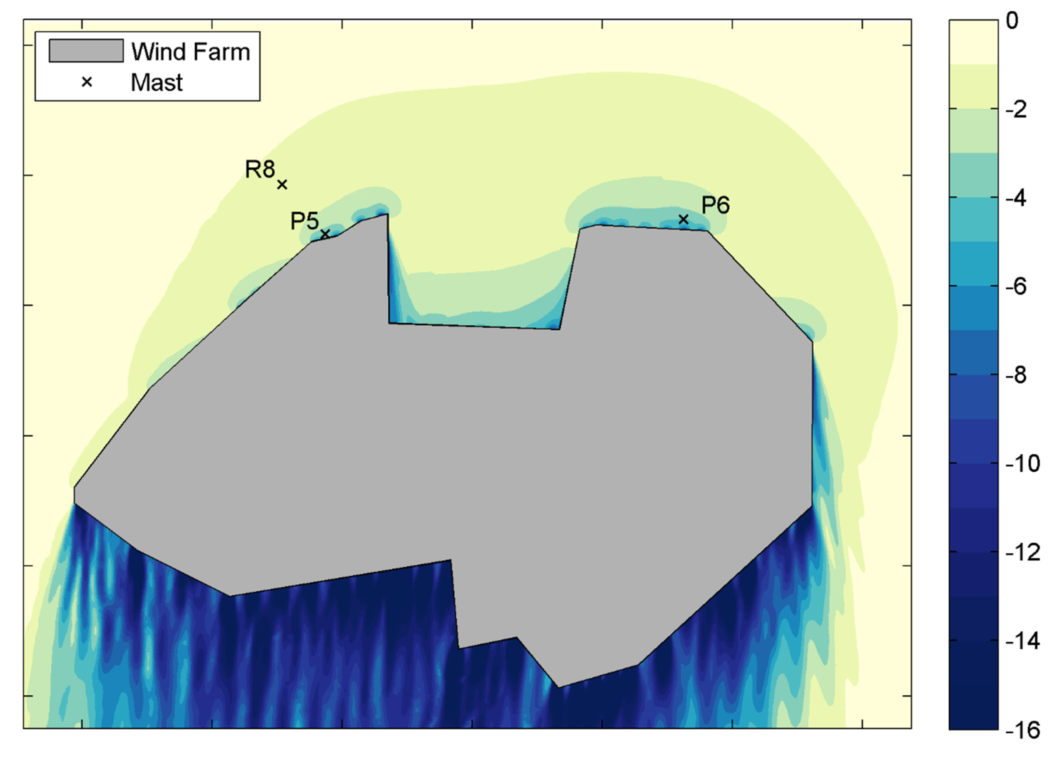
Figure 10.
Measured and predicted values for each perimeter-reference mast pair at Wind Farm C. The red “S” below each measured result denotes that reflects a statistically significant change in the wind speed relationship between Px and R8—with a p-value below 2 × 10⁻⁶. The black error bars represent the standard error of measured .

Figure 11.
Turbine interaction loss and wakes-only prediction bias at three onshore wind farms (A, B, and C) as derived from RANS simulations of the 30° sector centered on 0°. is the turbine interaction loss as would be predicted using the wakes-only approach. is the neglected portion of the total turbine interaction loss, and is the resulting energy prediction bias. The values correspond to the wind farm turbines operating on the plateaus of their respective Ct curves.

© 2018 by the authors. Licensee MDPI, Basel, Switzerland. This article is an open access article distributed under the terms and conditions of the Creative Commons Attribution (CC BY) license (http://creativecommons.org/licenses/by/4.0/).
Share and Cite
MDPI and ACS Style
Bleeg, J.; Purcell, M.; Ruisi, R.; Traiger, E. Wind Farm Blockage and the Consequences of Neglecting Its Impact on Energy Production. Energies 2018, 11, 1609. https://doi.org/10.3390/en11061609
AMA Style
Bleeg J, Purcell M, Ruisi R, Traiger E. Wind Farm Blockage and the Consequences of Neglecting Its Impact on Energy Production. Energies. 2018; 11(6):1609. https://doi.org/10.3390/en11061609
Chicago/Turabian StyleBleeg, James, Mark Purcell, Renzo Ruisi, and Elizabeth Traiger. 2018. "Wind Farm Blockage and the Consequences of Neglecting Its Impact on Energy Production" Energies 11, no. 6: 1609. https://doi.org/10.3390/en11061609
Note that from the first issue of 2016, this journal uses article numbers instead of page numbers. See further details here.