Real-Time Decision Making in First Mile and Last Mile Logistics: How Smart Scheduling Affects Energy Efficiency of Hyperconnected Supply Chain Solutions


Institute of Logistics, University of Miskolc, 3515 Miskolc, Hungary
Energies 2018, 11(7), 1833; https://doi.org/10.3390/en11071833
Submission received: 15 June 2018
/
Revised: 3 July 2018
/
Accepted: 8 July 2018
/
Published: 12 July 2018
(This article belongs to the Special Issue Energy Efficiency in the Supply Chains and Logistics)
Abstract
:Energy efficiency and environmental issues have been largely neglected in logistics. In a traditional supply chain, the objective of improving energy efficiency is targeted at the level of single parts of the value making chain. Industry 4.0 technologies make it possible to build hyperconnected logistic solutions, where the objective of decreasing energy consumption and economic footprint is targeted at the global level. The problems of energy efficiency are especially relevant in first mile and last mile delivery logistics, where deliveries are composed of individual orders and each order must be picked up and delivered at different locations. Within the frame of this paper, the author describes a real-time scheduling optimization model focusing on energy efficiency of the operation. After a systematic literature review, this paper introduces a mathematical model of last mile delivery problems including scheduling and assignment problems. The objective of the model is to determine the optimal assignment and scheduling for each order so as to minimize energy consumption, which allows to improve energy efficiency. Next, a black hole optimization-based heuristic is described, whose performance is validated with different benchmark functions. The scenario analysis validates the model and evaluates its performance to increase energy efficiency in last mile logistics.
1. Introduction
Energy efficiency has become a primary energy policy goal in the world and the research of energy efficiency of supply chain has a great scientific potential [1]. Energy efficiency is an inherent part of Industry 4.0. Power management means that for production and service networks more than energy efficiency, costs, and quality. Energy efficiency is the key factor for economic and social development, ranging from the entities which develop energy efficient measures to everyone in society [2]. The increased intensity of cooperation among supply chain members based on Industry 4.0 technologies offers an enormous potential. In networking, particularly hyperconnected supply chains, in addition to the traditional coordination of the operations, the members may also share their information, financial, and technical resources [3]. As Kevin Morin said in an interview: “Over time, as energy becomes an increasingly digital given with sensors, while also becoming more decentralized with energy coming from a local solar photovoltaic, wind or microgrid system, users will have even more control and ability to manage their energy usage” [4]. It means that today the design and operation of supply chain solutions, external systems, and in-plant processes are more complicated than in the future of Industry 4.0, when digitalized energy will make it possible to control and optimize energy consuming resources.
First mile logistics is the first stage and last mile logistics is the last stage of the supply chain and comprises a significant part of the total delivery cost and energy consumption. Industry 4.0 technologies make it possible to reduce order fulfillment time through real-time processing of open task in a network of package delivery service providers. Therefore, the improvement of first mile and last mile logistics and a significant externalities reduction are very important challenges for researchers [5]. Based on the importance of the energy efficiency of first mile and last mile services represented by package delivery service providers, it can be concluded that the research topic is quite relevant. The increasing importance of cost, resource and energy efficiency in supply chain solutions and the intention to find design and operation strategies supported by real-time decisions were a motivation for writing this paper. After this introduction, the remaining parts of the paper are divided into five sections. Section 2 presents a systematical literature review to summarize the research background. Section 3 presents the model framework and mathematical model of first mile and last mile supply chain including real-time decision of scheduling and assignment to increase energy efficiency. Section 4 presents an enhanced version of black hole heuristics. This section describes new operators for the heuristics and their increased performance is validated using benchmarking functions. Section 5 presents the numerical analysis of real-time decision making in first mile and last mile logistics focusing on the energy efficiency. Conclusions and future research directions are discussed in the last section.
2. Literature Review
Within the frame of this chapter the following questions are answered with a systematic literature review: Who is doing what? Who first did it or published it? What are research gaps?
2.1. Conceptual Framework and Review Methodology
Our used methodology of systematic literature review includes the following aspects [6]:
- formulate of research questions;
- select sources to the literature, like Scopus, Science Direct, Web of Science ResearchGate, or Google Scholar;
- reduce the number of articles by reading them and identify the main topic;
- define a methodology to analyze the chosen articles;
- describe the main scientific results;
- identify the scientific gaps and bottlenecks.
Firstly, the relevant terms were defined. It is a crucial phase of the review because there are excellent review articles in the field of supply chain management and we didn’t want to produce an almost similar review. We used the following keywords to search in the Scopus database: “energy efficiency” AND “logistics”. Initially, 466 articles were identified. This list was reduced to 231 articles selecting journal articles only. Our search was conducted in May 2018; therefore, new articles may have been published since then.
2.2. Descriptive Analysis
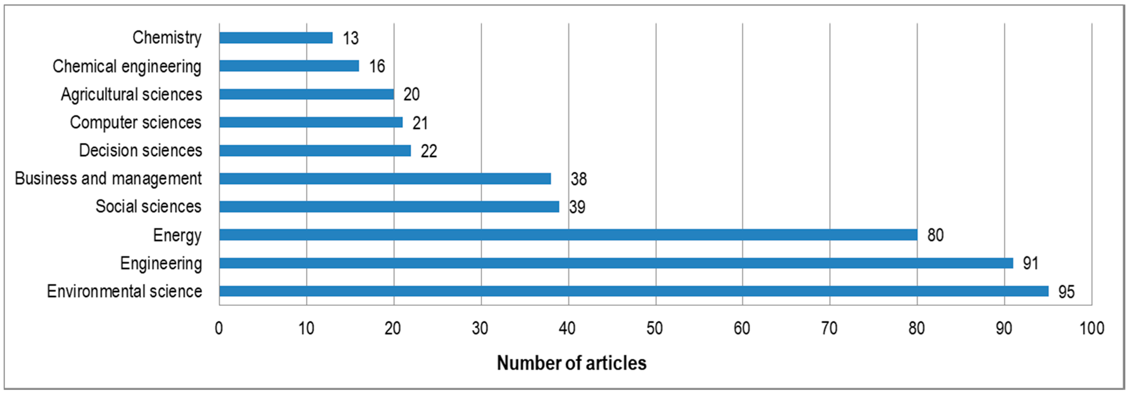
The reduced articles can be classified depending on the subject area. Figure 1 shows the classification of these 231 articles considering 10 subject areas. This classification shows the majority of environmental sciences, engineering, and energy, and defines the importance of computational methods related to decision sciences.
As Figure 2 demonstrates, the energy efficiency in logistics and supply chain has been researched in the past 20 years. The first article in this field was published in 1998 in the field of energy efficiency in passenger transportation [7] and it was focusing on the proportion of different transportation method. The number of published papers increased in the last eight years; this shows the importance of this research field.
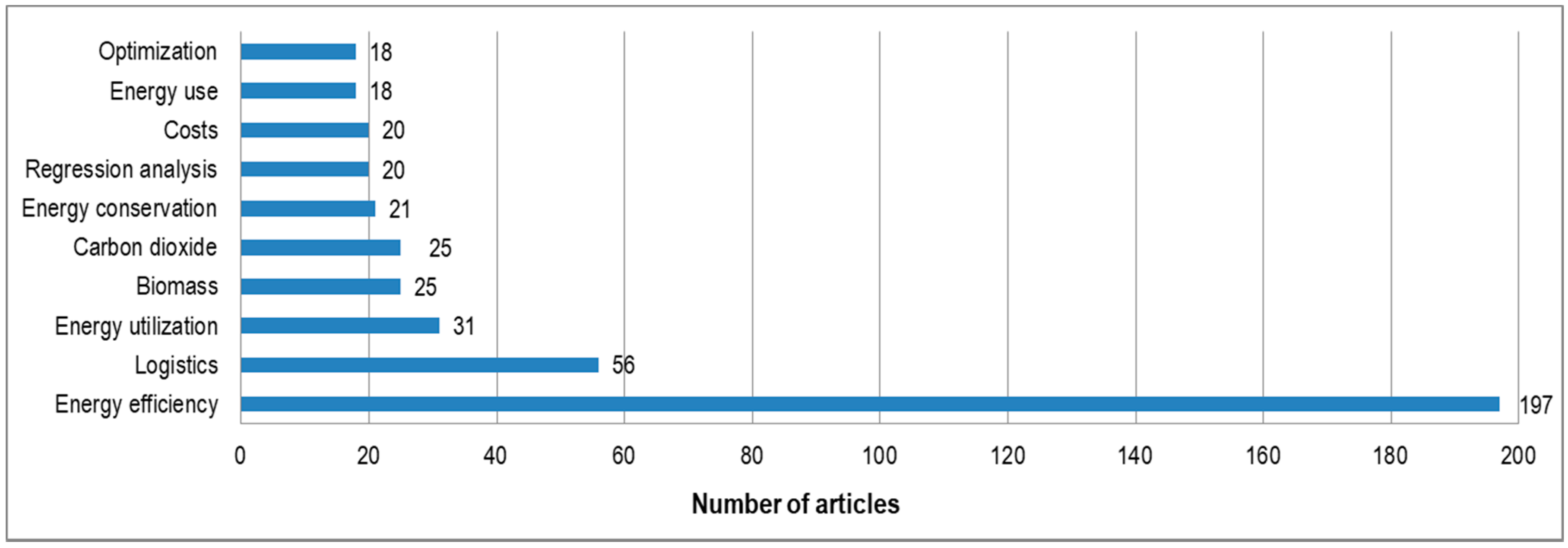
The distribution of the most frequently used keywords is depicted in Figure 3. As the keywords show, the design of energy efficiency of supply chain solutions is based on optimization methods and cost is the most important constraints.
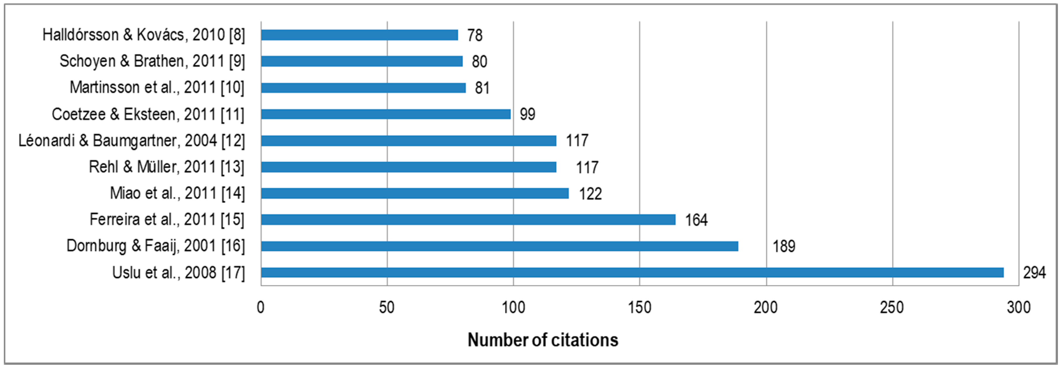
Articles were analyzed from scientific impact point of view. The most usual form to evaluate articles from scientific impact point of view is the citation. Figure 4 shows the 10 most cited articles with their number of citations [8,9,10,11,12,13,14,15,16,17].
In the following step, the 231 articles were reduced after reading the abstracts. We excluded articles whose topic did not match our interest and cannot be addressed to the energy efficiency of supply chain solutions. After this reduction, we got 45 articles.
2.3. Content Analysis
The literature introduces a wide range of methods used to solve problems of energy efficiency in supply chain domain, like decision support systems, heuristic optimization, statistical approaches, measurement, aggregate methods, or empirical studies. Hierarchical linear models were used to validate that greater urbanization, transport-related energy consumption, and transportation-sector greenhouse gas emissions have a great impact on each other [18]. Decision support tools, like the Synchromodal Supply Chain Energy Analysis (SSCEA) tool [19], make it possible to analyze and customize supply chain model and analyze their environmental and economic effects. Comparing and measuring logistic systems and processes against others is a good way to gain insights into measures, performance, and practices in a way that can rapidly improve the energy efficiency [20]. Statistical approaches using augmented Dickey–Fuller test, Johansen co-integration test, or impulse response can help to validate that energy efficiency, energy structure, and product remanufacturing rate are more capable of inhibiting reverse logistics carbon footprint [21]. Studies validate the usability of aggregated methods to improve operational energy efficiency in short sea container shipping, where appropriate vessel sailing speed, port time/sailing time ratio, and cargo capacity utilization need to be taken into account [9]. In the case of real supply chain solutions, empirical analysis can also be used. Researchers analyzed the impact of energy management systems on carbon and corporate performance with data from German automotive suppliers using empirical analysis [22]. The optimization is a very powerful tool in the case of both external logistic systems, supply chains, and intralogistics systems [23]. Another approach is the measuring. On the basis of measuring environmental performance across a green supply chain, researchers validated different regression models for resource conservation, reduction of hazardous waste, and reduction of emission of greenhouse gases [24]. The value-stream mapping method has proven itself to be the best practice tool to generate energy value-streams in production and logistics in respect to time- and energy-consumption [25]. Supply chain coordination enables additional opportunities that the individual approach hinders. For instance, an alternative supply method for raw material in manufacturing led to greening supply chain [26].
The measurement of supply chain and logistics solutions is performed allowing to quantify availability, flexibility, efficiency, and plasticity indicators [27]. Several scenarios related with energy efficiency of supply chain solutions were assessed and evaluated in order to compare the effects of technology, organization, infrastructure, policy, and finance. Case studies show that energy efficiency is a crucial problem in all areas of economy. A Stockholm pilot study shows that night-time deliveries increase the energy efficiency of urban goods delivery [28]. A South Korean case study describes that urban planning for optimal city size and characteristics with sufficient financing can lead to reduced logistics-related energy consumption [18]. The results of a study including 27 European countries over a period of 2007–2014 show that logistics performance index significantly increases GDP per unit of energy use, health expenditures, and renewable energy source, and decreases carbon emissions [29]. Based on data from 108 German automotive suppliers, a study described that the implementation of an Energy Management System has a (positive) effects on their practices and performances [22]. Measuring and improving operational energy efficiency is important in all supply chain solutions, like road, rail, water [9], and air. A Beijing pilot study examines the role of bicycles and tricycles for package delivery, food and beverage distribution, and waste and recycling services. The study shows that motorized alternatives to the tricycle are uncompetitive in terms of energy efficiency [30]. Intermediate and flexible transport, logistics, and supply chain schemes, operated by eco-friendly vehicles support the achievement of high standards of energy efficiency and environmental quality [31]. The extension of the green corridor system to all nodes of the shipping line and other transport modes in the case of a port in Spain led in the long run to a carbon-neutral green corridor [32].
The objective functions and indicators of design of supply chains from energy efficiency point of view can include a wide range of aspects, like capacity utilization, CO2 emission, fuel replacing, cooperation with stakeholders, taxes, or policies. Research results suggest that energy efficiency of supply chain solutions can be increased by enhanced utilization of capacity [33]. Studies show that unmanned aerial vehicles have potential effectiveness to reduce CO2 emissions compared to conventional transportation solutions [34]. Policies have a great impact on the performance. Policies that shift deliveries from peak hours to off-peak hours have the potential to increase the scheduling flexibility, delivery reliability and energy efficiency of carriers and recipients through the introduction of additional off-peak hours [28]. Replacing the heavy fuel oil by low sulfur fuel oil and shore power can lead to increased energy efficiency as shown in a study focusing on a case study of the port of Shenzhen. The proposed approach can be generalized for other ports [35]. Investigations have pointed out that logistic organizations and supply chain networks can achieve environmental goals. Therefore, it is necessary that companies develop a concrete environment-friendly orientation, based on the respect of market’s requests and environmental regulations and cooperate with their stakeholders [36]. A logistic-induced energy economic hybrid model combining top-down and bottom-up modeling and introducing revised logistic curves for enriching technical details validated that optimal carbon taxes can help to achieve the voluntary goal of reducing carbon intensity [37]. Examples show that in order to affect transport demand and total energy consumption, the focus should be shifted from single shipments to the analysis of complete supply chain solutions, including purchasing, in-plant supply, distribution, and inverse processes [38]. The energy efficiency of supply chain solutions can be influenced in three levels: operational, tactical, and strategic (conceptual) level [8]. Developed Geographic Information System (GIS)-based decision support program can be a unique tool assisting suppliers in making comprehensive decisions on organizational options for the most suitable, most energy efficient transportation [39].
The energy efficiency research of supply chain solutions and logistic systems covers a wide range of production and service processes as follows: city logistics [40,41,42], competing supply chains [43], container shipping [9,44], conveyor systems [45,46], intralogistics [47,48,49,50,51,52], last mile logistics [53], logistic centres [54], manufacturing plants [55], port logistics [35,36,56], regional distribution [57], reverse logistics [21], synchromodal supply chain [19], urban mobility [41], vaccine supply chain [58], and vehicle fleet management [59]. Figure 5 gives an overview of popular approaches used in design of supply chains and logistic systems focusing on energy efficiency, including models, research fields, and case studies and scenarios [60].
More than 50% of the articles were published in the last five years. This result indicates the scientific potential of the research on energy efficiency of supply chain. The articles that addressed the optimization of supply chain and logistics systems from energy efficiency and energy utilization point of view are focusing on conventional supply chain solutions, but few of the articles have aimed to research the design and operation of first mile and last mile supply chain solutions.
Therefore, first mile and last mile supply still needs more attention and research. It was found that heuristic and metaheuristic algorithms are important tools for design and operation of complex supply chain solutions since a wide range of models determines an NP-hard (non-deterministic polynomial-time hardness) optimization problem. According to that, the main focus of this research is the modelling and optimization of first mile and last mile supply chain solutions focusing on energy efficiency, also taking into account the real-time scheduling possibilities based on Industry 4.0 technologies.
The main contribution of this article includes: (1) the model of real-time operation of first mile and last mile supply chain solutions that include scheduling and assignment problems; (2) black hole algorithm based heuristic algorithm to solve real-time decision making problem of first mile last mile supply chain from energy efficiency point of view; (3) analysis of new operators for standard black hole optimization to increase the performance of the algorithm from speed of convergence point of view; and (4) computational results of the real-time decision making models with different datasets.
3. Model of Real-Time Decision Making in Last Mile Logistics to Increase Energy Efficiency
In traditional parcel delivery services (PDS), the first mile and last mile operations are separated: delivery of packages is performed in the morning while the pickup operations of new packages are scheduled in the afternoon. It means that the first mile and last mile operations are sequenced. The model framework of the real-time decision making of parcel delivery services makes it possible to analyze the performance of logistics of deliveries and pickup operations in order to increase the energy efficiency of transportation and other material handling operations. Table 1 shows the units of measures used in the model.
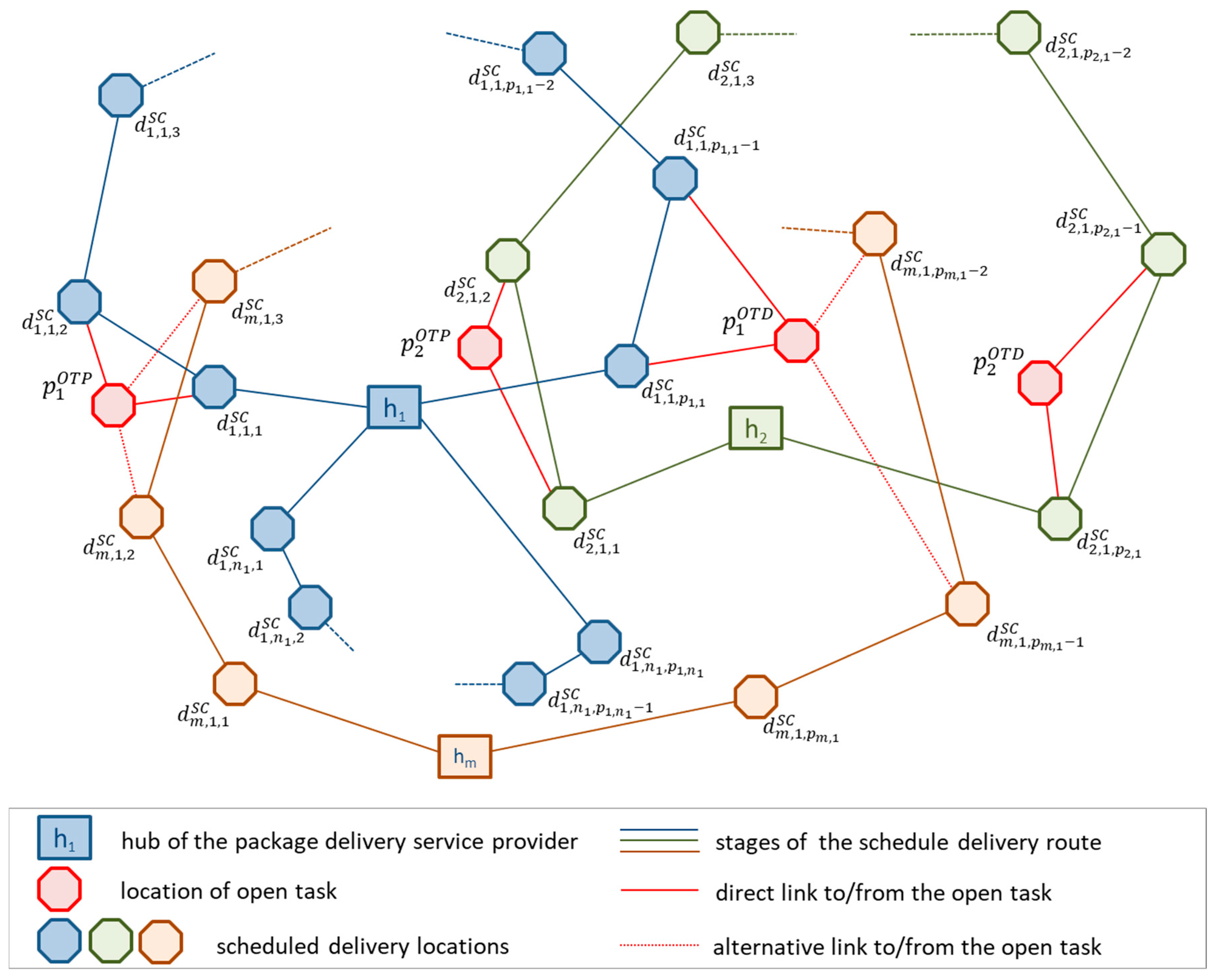
The model shown in Figure 6 includes three different types of deliveries: (1) scheduled deliveries, which are scheduled and assigned to delivery trucks; (2) open tasks with known delivery destinations, which are not scheduled and assigned to delivery trucks and routes; (3) open tasks with unknown open delivery destination, which are not scheduled and assigned to delivery trucks and routes. The supply chain model includes m parcel delivery services with scheduled routes and delivery locations, where i is the PDS ID and j is the route ID. There are open tasks which have to be picked up and if possible delivered to the known destination. The supply chain of a parcel delivery service system includes hubs and spokes represented by parcel delivery centers, where picked up packages can be stored if the delivery with point-to-point transport is not possible or the destination is unknown while picking up. The decision variables of this model are the following: assignment of open tasks (new packages) to delivery service provider and delivery route, scheduling of pickup, and delivery operations of new tasks. The integration of assignment and scheduling problem represents an NP-hard optimization problem.
With this in mind, we define the following parameters describing the layout of the hyperconnected first-mile/last-mile supply chain:
- is the position of the delivery point k of the scheduled delivery route j of parcel delivery service provider (PDSP) i where , and ;
- is the hub’s position of PDSP i;
- is the position of the pickup point of the open task f, where ;
- is the position of the destination of the open task f.
The objective function of the problem describes the minimization of energy use of the whole delivery process:
where is the energy usage of delivery of scheduled deliveries without any assigned open task, is the energy usage from the hub to the first destination and from the last destination to the hub, is the energy usage of pickup operations of open tasks and is the energy usage of delivery operations of open tasks.
The first part of the energy usage function (1) includes the sum of energy usage of scheduled delivery routes without assignment of open tasks, where the energy usage is a function of loading of package delivery trucks and the length of routes depending on the location of delivery points:
where is the specific energy usage of package delivery truck of PDSP i through scheduled delivery route j, is the load of the delivery truck of PDSP i through scheduled delivery route j passing delivery point k, is the length of the transportation route of PDSP i through scheduled delivery route j between destination k and destination k + 1.
The second part of the energy usage function (1) includes the energy usage from the hub to the first destination and from the last destination to the hub:
The third part of the energy usage function (1) includes the energy usage of pickup operations of assigned open tasks as a sum of the energy usage among delivery point k, pickup point of the open task f and delivery point k + 1:
where
and
where is the number of assigned open tasks to the delivery route j of PDSP i, is the assignment matrix of pickup operations of open tasks to scheduled delivery routes as a decision variable, is the transportation length between the scheduled destination k and the pickup destination of the open task f.
The fourth part of the energy usage function (1) includes the energy usage of delivery operations of assigned open tasks as a sum of the energy usage among delivery point k, delivery location of the open task f and delivery point k + 1:
where
and
where is the assignment matrix of delivery operations of open tasks to scheduled delivery routes as decision variable. If the pickup of open task f is assigned to delivery route j of PDSP i passing delivery point k, then . If the delivery of open task f is assigned to delivery route j of PDSP i passing delivery point k, then .
The solutions of the above described integrated scheduling and assignment problem are limited by the following three constraints related to time window and capacity of package delivery trucks:
Constraints 1: We can define a timeframe for each scheduled delivery operation and it is not allowed to exceed the upper and lower limit of this timeframe.
where is the scheduled pickup/delivery time at delivery point k of route j of PDSP i without added open tasks, is the lower limit of pickup/delivery time at delivery point k of route j of PDSP i, is the upper limit of pickup/delivery time at delivery point k of route j of PDSP i, is the traveling time between delivery point k of route j of PDSP i and pickup location of the open task f, is the traveling time between the assigned open task f and the succeeding delivery point k of route j of PDSP i.
Constraints 2: We can define a timeframe for each open task and it is not allowed to exceed the upper and lower limit of pickup and delivery operation time:
where is the lower limit of pickup time of the assigned open task f, is the upper limit of pickup time of the assigned open task f, is the lower limit of delivery time of the assigned open task f, is the upper limit of delivery time of the assigned open task f.
Constraints 3: The capacity of package delivery trucks is limited, so it is not allowed to exceed its loading capacity. The actual loading capacity at the scheduled destination k of package delivery truck assigned to delivery route j of PDSP i can be calculated as follows:
where is the maximum capacity of package delivery truck assigned to delivery route j of PDSP i. If there is a difference between the value of open task at the pickup point and the destination, then this constraint can be written as follows:
The decision variables have two different types: the decision variable of the assignment problem is a binary matrix, while the decision variable of the scheduling problem is a matrix with real values. The assignment matrix (15) defines the scheduling of open tasks, so we have one real decision variable, while the scheduling matrix is a virtual decision variable.
4. Black Hole Algorithm-Based Optimization
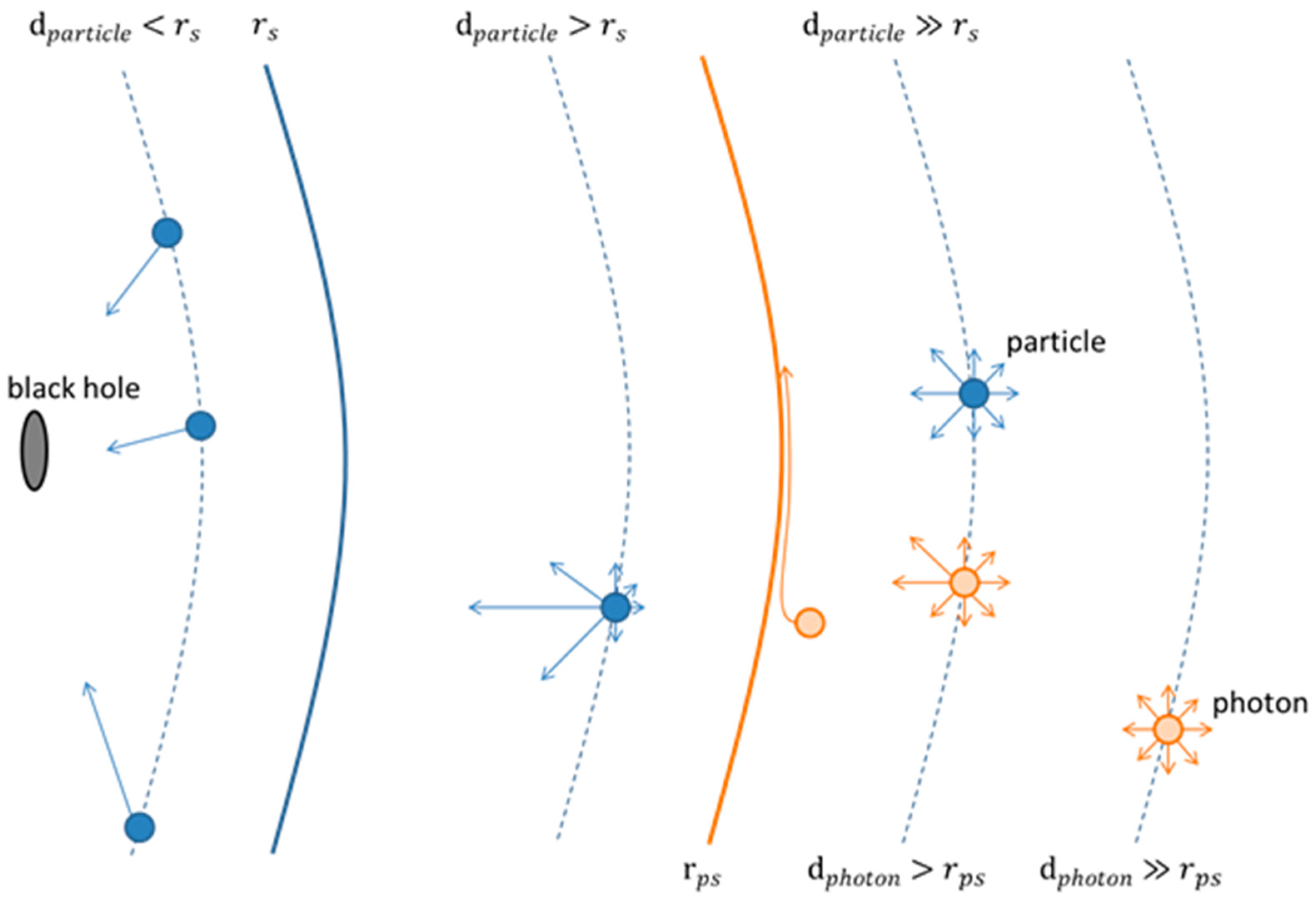
The idea of black holes was established in the 18th century by John Michel and Pierre Simon de Laplace, and the first black hole was recognized by John Wheeler in 1967 [61,62]. A common type of black hole is created by dying stars with very large masses, when the gravity force won against pressure. There are three types of black holes depending on their mass: stellar black holes, supermassive black holes, and miniature black holes. In a black hole, gravity force pulls so much that nothing, not even particles, light or radiation can escape from it. But black holes are not giant cosmic vacuum cleaners, because the gravity force of a black hole is extremely high if a particle is extremely close. This boundary is the so-called event horizon. The radius of the event horizon is the Schwarzschild radius, which can be calculated as follows:
where g is Newton’s gravitational constant, M is the mass of the object and c is the speed of light. Inside the event horizon, the gravity force drags all particles back and prevents it from escaping. There is another special sphere around non-spinning black holes. The photon sphere is a spherical region; photons reaching this region are forced to travel in orbits. The radius of photon sphere can be calculated as follows:
The environment of black holes can be analyzed, but the black holes are invisible, because light cannot escape. If the distance between a particle (star, proton, electron, photon, etc.) is much higher than the Schwarzschild radius, then the particle can move in any directions. If this distance is larger than the Schwarzschild radius, but this difference is not too much, the space-time is deformed, and more particles are moving towards the center of the black hole than in other directions. If a particle reaches the Schwarzschild radius, then it can move only towards the center of the black hole (Figure 7). The black hole optimization is based on this phenomenon of black holes [63].
Black hole algorithm (BHA) is inspired by this phenomenon and belongs to the swarm intelligence paradigm using adaptive strategies to search and optimize. Black hole algorithm can be defined as a sub-field of particle swarm optimization and they are inspired by physical laws, like gravitation search [64], intelligent water drop [65], or simulated annealing [66]. Other types of heuristic optimization algorithms are inspired by living bodies, like bacterial algorithm [67], bat algorithm [68], artificial bee colony algorithm [69], firefly algorithm [70], and ant colony algorithm [71].
Black hole optimization (BHO) can be used to solve binary [72,73], hybrid binary [74], discrete [75], and real problems [63]. The black hole algorithms can solve different NP-hard optimization problems related to electric power systems [76], scheduling in automotive industry [77], pattern synthesis ion radio science [78], earth sciences [79] logistics and supply chain [80], nondestructive testing of wiring networks [81], and electrochemical machining [82].
The first phase of the black hole optimization is the so called big-bang, which is the initialization phase of location and velocity of stars in the search space. Each star represents a possible solution of the optimization problem, where location in the n-dimensional search space represents the value of the decision variables. The generated stars have to be inside the boundaries of the search space.
The second phase of the algorithm is the evaluation of the stars representing potential solutions. The stars are evaluated with the value of the objective functions after moving towards the black hole.
The third phase of the algorithm is to choose the heaviest star with the best value of objective function to represent the black hole. This star with the highest gravity force is the center of the movement of stars.
The fourth phase of the algorithm is the moving (swarming) of stars towards the black hole. We can define two different types of movement: in the first case, only the gravity force between star and black hole has impact on the movement of the star, while in the second case, the gravity force among all stars are taken into consideration. The second case is performed through the gravity search algorithm.
The movement process has to be performed so that the new location of the star after the movement is inside the search space, because limitations of decision variables have to be taken into consideration. Stars reaching the event horizon are absorbed and a new star is generated in the search space. It is important to schedule the evaluation of stars reaching the event horizon. If the candidate solution represented by the star reaching the event horizon is not evaluated before absorbed, then it could happen that we lost a better solution than the solution represented by the black hole, especially in the case if the global optimum of the problem is inside the event horizon of the current black hole. If we evaluate stars reaching the event horizon, the evaluated star can become the new black hole and the best solution among the candidate stars get nearer to the global optimum (Figure 8).
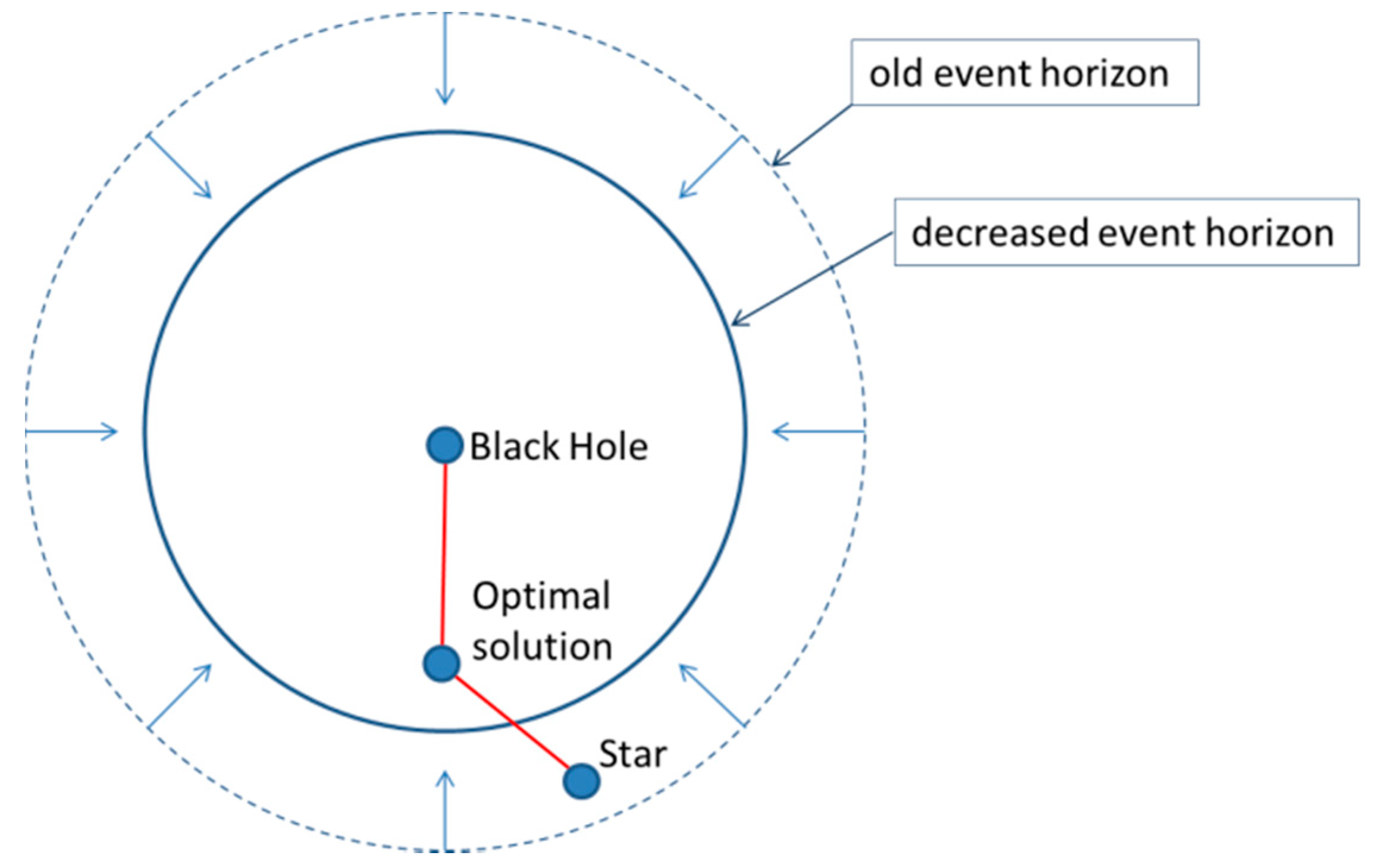
The Schwarzschild radius can be taken into consideration either as a constant value or as a permanently decreased value. If we take into consideration the Hawking radiation, then the black hole lost weight and the radius of the event horizon get smaller and smaller. The permanently decreased event horizon makes it possible to prevent the absorption of stars near the optimum of the objective function (Figure 9). The Schwarzschild radius can be calculated depending on the gravity force of the black hole, stars, and the current iteration step as follows:
where is the number of the current iteration step.
The application of Hawking radiation is another possible way to reach optimal solution near the black hole, inside the event horizon. Hawking verified that object can escape from a black hole and black holes mass can reduce [83]. This mass reduction has an impact on the gravity force of the black hole. Using this idea, it is possible to change the position of the black hole in the search space using the following calculation:
where influences the possible shift of the black hole. In the big-bang phase, the best option is to use uniform distribution to generate stars. After absorption of a star inside the event horizon, there are different ways to generate new stars. We can generate the new stars either uniformly or using a special, discrete, or continuous distribution function [84]. Figure 10 shows an example of performing generation of new stars with a discrete distribution. In this case .
The stars in the 1st sphere are called lucky stars. It is important that
where the possibility of uniformly generation of a new star instead of the absorbed one is
As termination criteria we can define either the upper limit of the number of iteration steps or the value of expected changes in the gravity force after the next iteration step.
On the basis of the abovementioned aspects of the black hole algorithm, it is possible to perform the optimization with different variations of the standard algorithm:
- standard BHA;
- BHA with permanently decreasing Schwarzschild radius;
- BHA with Hawking radiation;
- BHA with Lucky stars;
- BHA with permanently decreasing Schwarzschild radius and Hawking radiation;
- BHA with permanently decreasing Schwarzschild radius and lucky stars;
- BHA with Lucky stars and Hawking radiation;
- BHA with permanently decreasing Schwarzschild radius, Hawking radiation, and lucky star.
The results of the evaluation of the performance of different BHA is demonstrated in Table 2.
As Table 2 shows, the decreased Schwarzschild radius, the Hawking radiation, and the lucky star options increase the performance of the standard black hole algorithm, so the DSR/LS/HR version of the BHA is used in the next chapter to optimize the real-time decision making problem in last mile logistics to increase the energy efficiency.
5. Scenario Analysis of Real-Time Decision Making in Last Mile Logistics Focusing on Energy Efficiency
Within the frame of this chapter, the performance of the abovementioned black hole algorithm-based heuristics is validated through the optimization of real-time decision making problem of last mile logistics focusing on energy efficiency. The model has two package delivery service providers, 17 scheduled destinations for three scheduled routes (Table 3), and two open tasks (Table 4) to be picked up and delivered.
Within the frame of scenarios, the fuel consumption depending on the weight of the loading is calculated as follows:
where is the specific additional fuel consumption depending on the loading weight. The unit of measure of the energy consumption is L/100 km. Within the frame of these scenarios the linear fuel consumption function was used with a fuel consumption of 9 L/100 km for empty package delivery trucks and 13 L/100 km for full package delivery trucks. The fuel consumption was measured with the used fuel quantity.
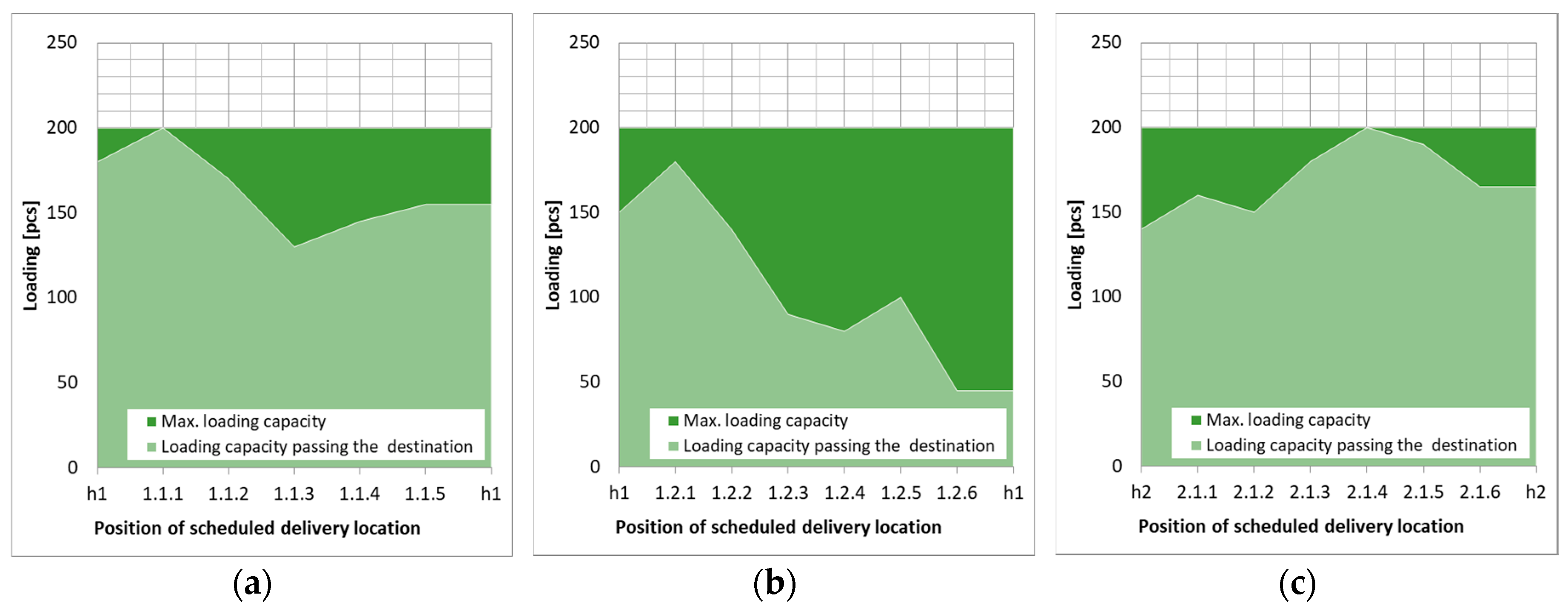
Figure 11 demonstrates the loading capacity of delivery routes of PDSPs. As the figures show, it is not allowed to exceed the loading capacity of delivery trucks without and with assigned open tasks. The loading capacity of delivery trucks is measured with pcs of standard postal boxes.
5.1. Scenario 1 with Non-Cooperating PDSPs, without Time Frame and Real-Time Scheduling
In the case of the first scenario, the time frame for pickup and delivery operations is not taken into consideration and open tasks are not scheduled real-time. The pickup and delivery operations of open tasks are performed by shuttle services of the PDSPs receiving the open task, because it is not possible to modify the scheduled routes (Figure 12a). In this case the total energy consumption is 38.246 L including 28.375 L energy consumption of the scheduled routes and 9.871 L energy consumption of shuttle services.
5.2. Scenario 2 with Cooperative PDSPs, without Time Frame and without Real-Time Scheduling
In the case of the second scenario, the time frame for pickup and delivery operations is not taken into consideration and open tasks are not scheduled real-time. The cooperation among PDSPs makes it possible to decrease the energy consumption, because pickup and delivery operations of open tasks are not performed by shuttle services receiving the open task. In this case, the total energy consumption is 35.265 L including 28.375 L energy consumption of the scheduled routes and 6.890 L energy consumption of shuttle services (Figure 12b).
5.3. Scenario 3 with Cooperative Partners, without Time Frame, without Loading Capacity Limit, and with Real-Time Scheduling
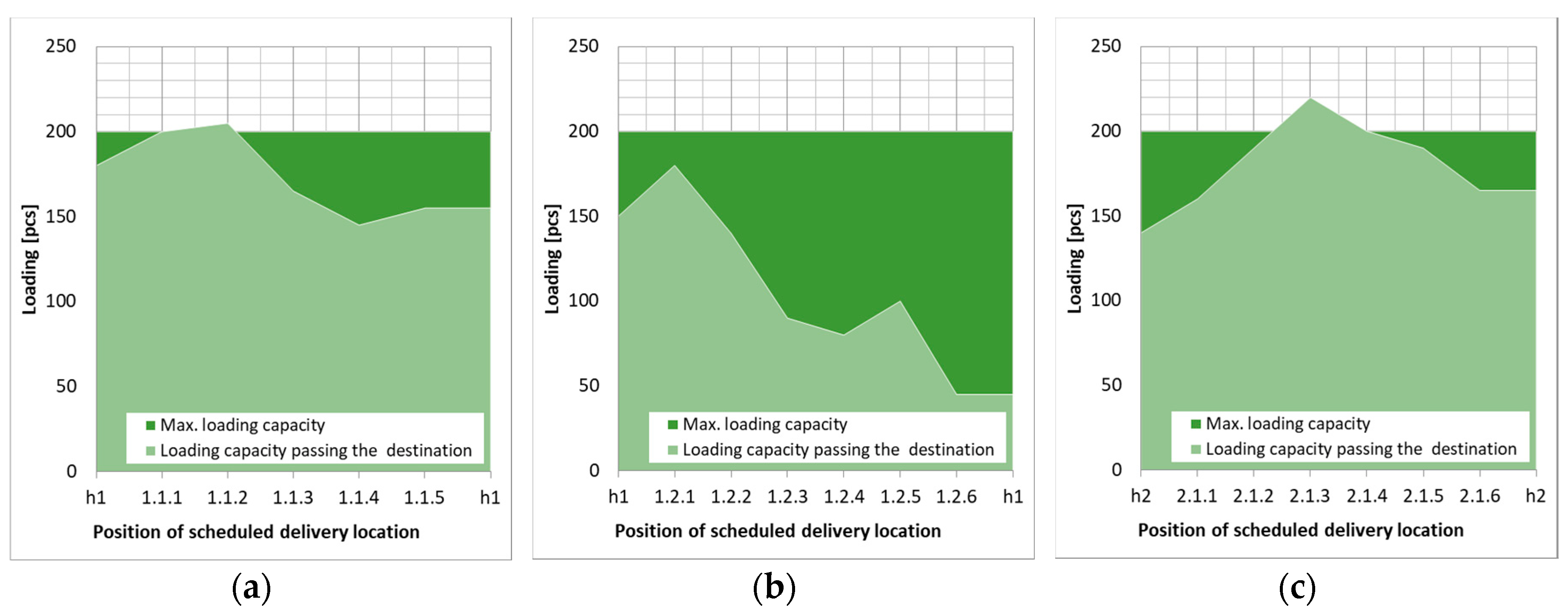
In the case of the third scenario, the time frame for pickup and delivery operations is not taken into consideration but open tasks are assigned to the scheduled routes. In this scenario, the loading capacity of trucks is not taken into consideration. In this case, the loading capacity of delivery trucks assigned to route 1 and 3 is exceeded, as Figure 13 shows. In this case the total energy consumption is 28.979 L including 22.658 L energy consumption of the scheduled routes and 6.321 L energy consumption of added routes for pickup and delivery of open tasks (Figure 14a).
5.4. Scenario 4 with Cooperative Partners, without Time Frame, with Limited Loading Capacity and Real-Time Scheduling
In the case of the fourth scenario, the time frame for pickup and delivery operations is not taken into consideration but it is not allowed to exceed the loading capacities of delivery trucks. In this case the open tasks are rescheduled (Figure 14b). As Figure 14 shows, the loading capacity of the delivery trucks is not exceeded after rescheduling pickup and loading operations of open tasks. In this case the total energy consumption is 30.97 L including 22.906 L energy consumption of the scheduled routes and 8.064 L energy consumption of added routes for pickup and delivery of open tasks.
5.5. Scenario 5 with Cooperative Partners, Time Frame, Limited Loading Capacity, and Real-Time Scheduling
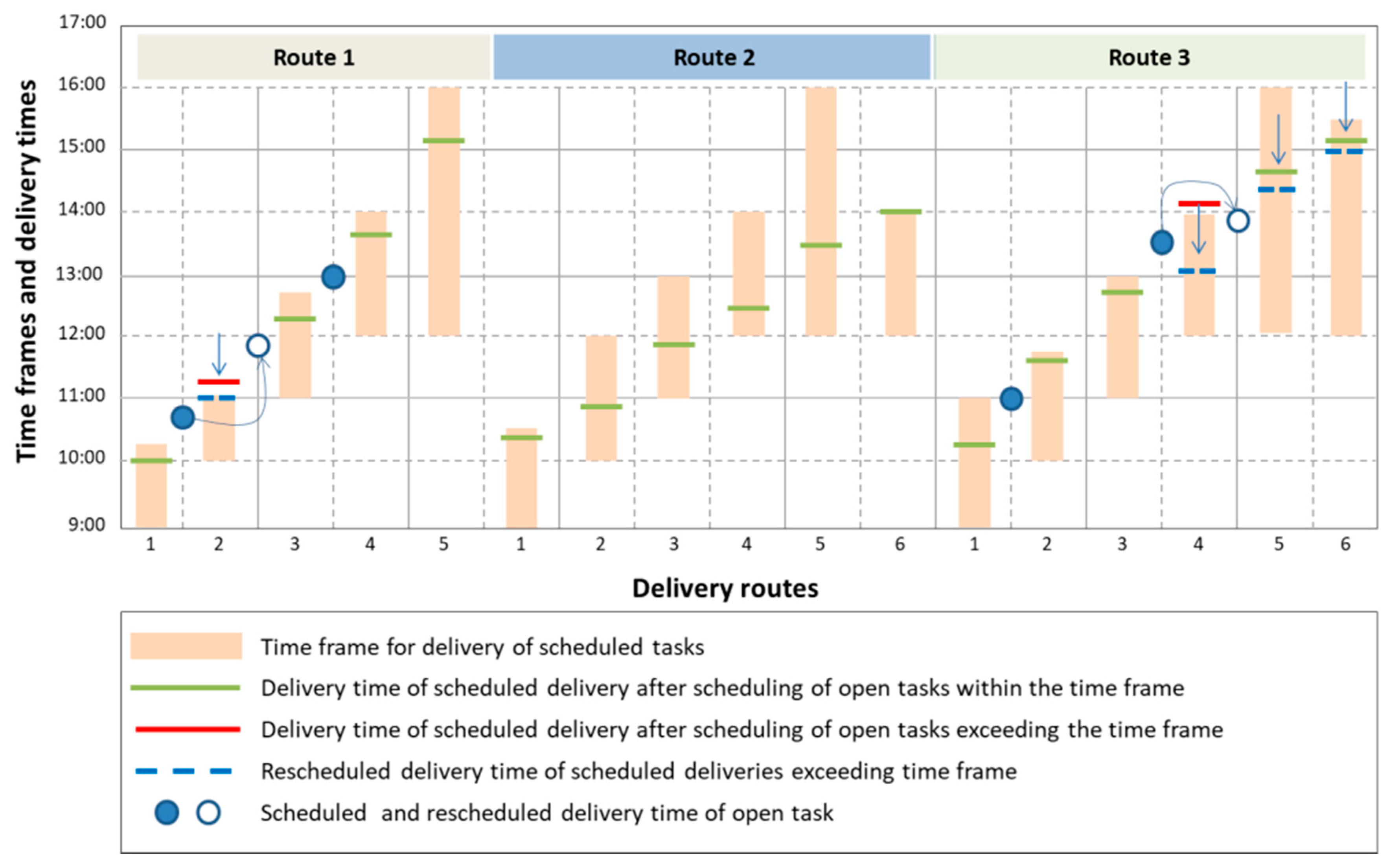
In the case of the fifth scenario, the time frame for pickup and delivery operations is taken into consideration and open tasks are assigned to the scheduled routes. The black hole algorithm-based heuristics resulted two different solutions, and loading capacity were not exceeded (Figure 15). The first solution represents the model, where time frames are not taken into consideration (Figure 16a), while the second solution includes the constrained time frame (Figure 16b). Taking into account the time frame, the total energy consumption is 28.979 L including 22.658 L energy consumption of the scheduled routes and 6.754 L energy consumption of added routes for pickup and delivery of open tasks. Figure 17 demonstrates the results of real-time scheduling.
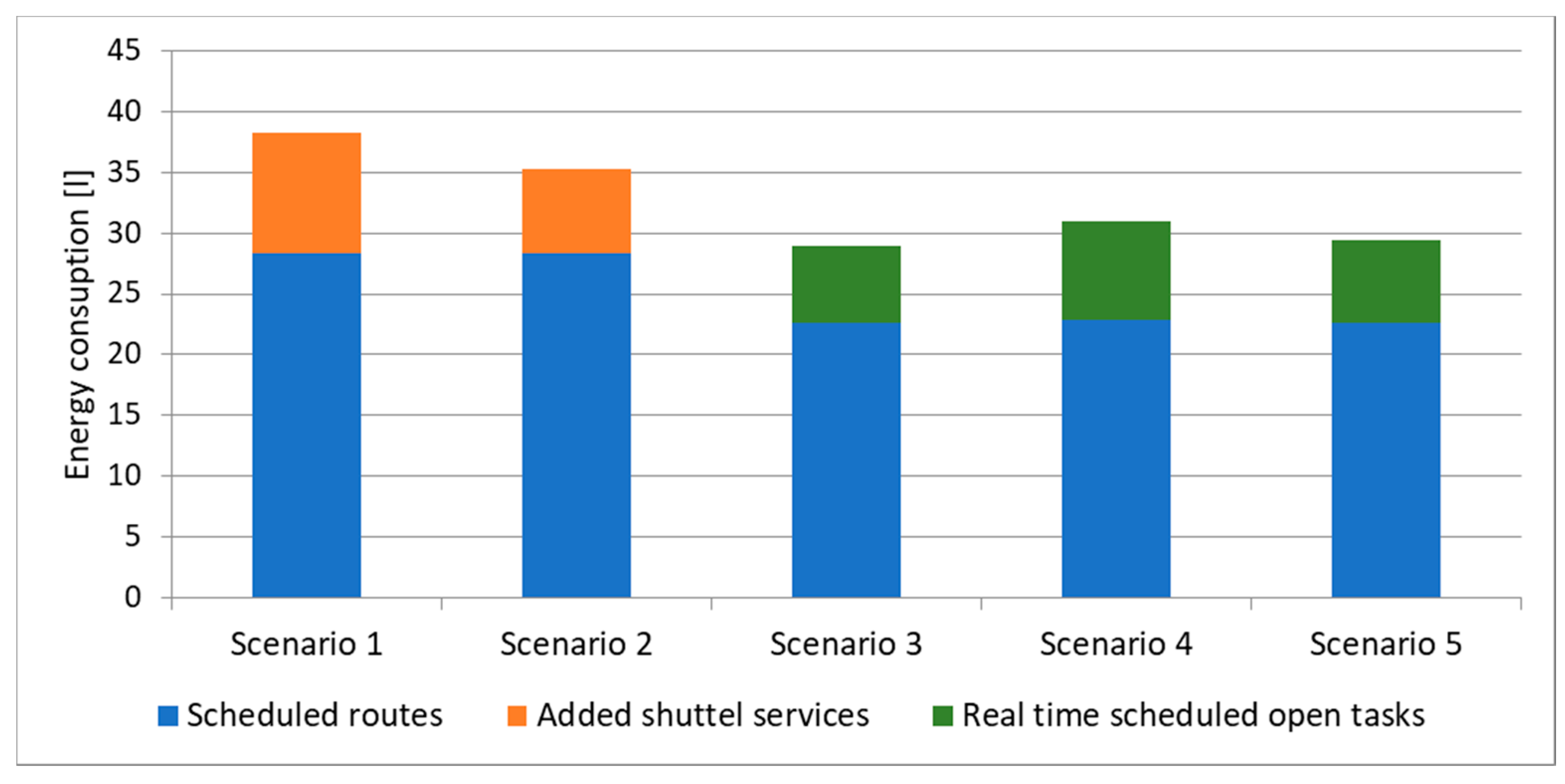
Figure 18 demonstrates the comparison of fuel consumption of the different assignment and scheduling solutions of the above described scenarios. However, scenario 3 has the lowest energy consumption, but in this scenario the pickup and delivery operations cannot be performed within the predefined timeframe. As the optimal solution, the results of scenario 4 have to be taken into consideration, because in this case the pickup and delivery operations can be performed within the time frame given by the customers.
6. Conclusions
It is common in logistics and supply chain that the objective of decreasing fuel consumption and increasing the energy efficiency is targeted at the level of operation of the supply chain’s members. The importance of cooperation has not been fully explored, but Industry 4.0 technologies and the Internet of Things paradigm led to the improvement of hyperconnected logistics and the abovementioned objective is targeted at strategic level. Energy efficiency is not extensively researched in the case of cooperative supply chain solutions. To try to fill this gap, this work has developed a methodology based on heuristic optimization of real-time scheduling of last mile logistics to minimize energy consumption, which allows to improve energy efficiency.
The model of first mile and last mile logistics focuses on the energy efficiency of cooperative package service providers. The described model represents an integrated optimization problem including assignment of open tasks to scheduled routes, scheduling of open tasks and rescheduling of existing delivery routes. The optimization problem, which is described by an objective function representing the minimization of energy consumption and constraints including loading capacity limits and time frame, is an NP-hard problem. For the solution of this problem, a black hole optimization-based heuristics was developed. The developed heuristic is an improved version of the standard black hole optimization; its increased performance is validated with benchmarking functions. The integrated optimization model of real-time scheduling of last mile logistics problem is solved with this heuristics. As the scenarios showed, cooperation makes it possible to increase energy efficiency through minimization of energy consumption.
Depending on the different constraints, different energy savings can be achieved. In the case of package delivery service providers, the time frame and the loading capacity of the package delivery trucks are important constraints, as the mentioned scenarios show, and they are influencing their reliability, availability, flexibility, and economic footprints.
The described model framework and the optimization approach makes it possible to support managerial decisions; not only the operation strategy of the running trucks but also the cooperation strategy of different package delivery service providers is influenced by the results of the above described contribution. Some recommendations for possible future studies are as follows: it would be helpful to develop approaches that beyond analyzing scheduling and assignment possibilities also consider other areas of interest, like human resource strategies, delivery truck sizing, or outsourcing possibilities. Another research direction is the analysis of stochastic models and the development of new heuristic methods to decrease the computation time of the algorithm for large-scale systems.
Funding
This research received no external funding.
Conflicts of Interest
The author declares no conflict of interest.
References
- Llorca, M.; Jamasb, T. Energy efficiency and rebound effect in European road freight transport. Transp. Res. Part A Policy Pract. 2017, 101, 98–110. [Google Scholar] [CrossRef]
- Marchi, B.; Zanoni, S. Supply Chain Management for Improved Energy Efficiency: Review and Opportunities. Energies 2017, 10, 1618. [Google Scholar] [CrossRef]
- Marchi, B.; Zanoni, S.; Ferretti, I.; Zavanella, L.E. Stimulating Investments in Energy Efficiency through Supply Chain Integration. Energies 2018, 11, 858. [Google Scholar] [CrossRef]
- Energy Efficiency as a Core Component of Industry 4.0—The Building Perspective. Available online: https://www.i-scoop.eu/industry-4-0/energy-efficiency-industry-4-0/ (accessed on 8 June 2018).
- Ranieri, L.; Digiesi, S.; Silvestri, B.; Roccotelli, M. A Review of Last Mile Logistics Innovations in an Externalities Cost Reduction Vision. Sustainability 2018, 10, 782. [Google Scholar] [CrossRef]
- Cronin, P.; Ryan, F.; Coughlan, M. Undertaking a literature review: A step-by-step approach. Brit. J. Nurs. 2008, 17, 38–43. [Google Scholar] [CrossRef] [PubMed]
- Ramanathan, R. Development of Indian passenger transport. Energy 1998, 23, 429–430. [Google Scholar] [CrossRef]
- Halldórsson, Á.; Kovács, G. The sustainable agenda and energy efficiency: Logistics solutions and supply chains in times of climate change. Int. J. Phys. Distrib. Logist. Manag. 2010, 40, 5–13. [Google Scholar] [CrossRef]
- Schøyen, H.; Bråthen, S. The Northern Sea Route versus the Suez Canal: cases from bulk shipping. J. Transp. Geogr. 2011, 19, 977–983. [Google Scholar] [CrossRef]
- Martinsson, J.; Lundqvist, L.J.; Sundström, A. Energy saving in Swedish households. The (relative) importance of environmental attitudes. Energy Policy 2011, 39, 5182–5191. [Google Scholar] [CrossRef]
- Coetze, L.; Eksteen, J. The internet of things—Promise for the future? An introduction. In Proceedings of the IST-Africa Conference, Gaborone, Botswana, 11–13 May 2011. [Google Scholar]
- Léonardi, J.; Baumgartner, M. CO2 efficiency in road freight transportation: Status quo, measures and potential. Transp. Res. Part D Transp. Environ. 2004, 9, 451–464. [Google Scholar] [CrossRef]
- Rehl, T.; Müller, J. Life cycle assessment of biogas digestate processing technologies. Resour. Conserv. Recy. 2011, 56, 92–104. [Google Scholar] [CrossRef]
- Miao, Z.; Grift, T.E.; Hansen, A.C.; Ting, K.C. Energy requirement for comminution of biomass in relation to particle physical properties. Ind. Crop. Prod. 2011, 33, 504–513. [Google Scholar] [CrossRef]
- Ferreira, J.G.; Andersen, J.H.; Borja, A.; Bricker, S.B.; Camp, J.; Cardoso da Silva, M.; Garcés, E.; Heiskanen, A.-S.; Humborg, C.; Ignatiades, L.; et al. Overview of eutrophication indicators to assess environmental status within the European Marine Strategy Framework Directive. Estuar. Coast. Shelf. Sci. 2011, 93, 117–131. [Google Scholar] [CrossRef]
- Dornburg, V.; Faaij, A.P.C. Efficiency and economy of wood-fired biomass energy systems in relation to scale regarding heat and power generation using combustion and gasification technologies. Biomass Bioenergy 2001, 21, 91–108. [Google Scholar] [CrossRef]
- Uslu, A.; Faaij, A.P.C.; Bergman, P.C.A. Pre-treatment technologies, and their effect on international bioenergy supply chain logistics. Techno-economic evaluation of torrefaction, fast pyrolysis and pelletisation. Energy 2008, 33, 1206–1223. [Google Scholar] [CrossRef]
- Lee, J.H.; Lim, S. The selection of compact city policy instruments and their effects on energy consumption and greenhouse gas emissions in the transportation sector: The case of South Korea. Sustain. Cities Soc. 2018, 37, 116–124. [Google Scholar] [CrossRef]
- Farahani, N.Z.; Noble, J.S.; Klein, C.M.; Enayati, M. A decision support tool for energy efficient synchromodal supply chains. J. Clean. Prod. 2018, 186, 682–702. [Google Scholar] [CrossRef]
- Stöhr, T.; Schadler, M.; Hafner, N. Benchmarking the energy efficiency of diverse automated storage and retrieval systems. FME Trans. 2018, 46, 330–335. [Google Scholar] [CrossRef]
- Sun, Q. Research on the influencing factors of reverse logistics carbon footprint under sustainable development. Environ. Sci. Pollut. Res. 2017, 24, 22790–22798. [Google Scholar] [CrossRef] [PubMed]
- Böttcher, C.; Müller, M. Insights on the impact of energy management systems on carbon and corporate performance. An empirical analysis with data from German automotive suppliers. J. Clean. Prod. 2016, 137, 1449–1457. [Google Scholar] [CrossRef]
- Hafner, N.; Lottersberger, F. Intralogistics systems - optimization of energy efficiency. FME Trans. 2016, 44, 256–262. [Google Scholar]
- Rao, P.H. Measuring Environmental Performance across a Green Supply Chain: A Managerial Overview of Environmental Indicators. Vikalpa 2014, 39, 57–74. [Google Scholar] [CrossRef] [Green Version]
- Müller, E.; Stock, T.; Schillig, R. A method to generate energy value-streams in production and logistics in respect of time- and energy-consumption. Prod. Eng. 2014, 8, 243–251. [Google Scholar] [CrossRef]
- Ferretti, I.; Zanoni, S.; Zavanella, L.; Diana, A. Greening the aluminium supply chain. Int. J. Prod. Econ. 2007, 108, 236–245. [Google Scholar] [CrossRef]
- Tamás, P. Innovative business model for realization of sustainable supply chain at the outsourcing examination of logistics services. Sustainability 2018, 10, 210. [Google Scholar]
- Fu, J.; Jenelius, E. Transport efficiency of off-peak urban goods deliveries: A Stockholm pilot study. Case Stud. Transp. Policy 2018, 6, 156–166. [Google Scholar] [CrossRef]
- Zaman, K.; Shamsuddin, S. Green logistics and national scale economic indicators: Evidence from a panel of selected European countries. J. Clean. Prod. 2017, 143, 51–63. [Google Scholar] [CrossRef]
- Zacharias, J.; Zhang, B. Local distribution and collection for environmental and social sustainability—Tricycles in central Beijing. J. Transp. Geogr. 2015, 49, 9–15. [Google Scholar] [CrossRef]
- Mancuso, P.; Costagli, G.; Casella, C. The “ELBA” project—Eco-friendly mobility services for people and goods in small Islands. WIT Trans. Ecol. Environ. 2013, 179, 1079–1090. [Google Scholar]
- Carballo-Penela, A.; Mateo-Mantecón, I.; Doménech, J.L.; Coto-Millán, P. From the motorways of the sea to the green corridors’ carbon footprint: The case of a port in Spain. J. Environ. Plan. Manag. 2012, 55, 765–782. [Google Scholar] [CrossRef]
- Wehner, J. Energy efficiency in logistics: An interactive approach to capacity utilization. Sustainability 2018, 10, 1727. [Google Scholar] [CrossRef]
- Figliozzi, M.A. Lifecycle modeling and assessment of unmanned aerial vehicles (Drones) CO2e emissions. Transp. Res. Part D Transp. Environ. 2017, 57, 251–261. [Google Scholar] [CrossRef]
- Yang, L.; Cai, Y.; Zhong, X.; Shi, Y.; Zhang, Z. A carbon emission evaluation for an integrated logistics system-a case study of the port of Shenzhen. Sustainability 2017, 9, 462. [Google Scholar] [CrossRef]
- Cosimato, S.; Troisi, O. Green supply chain management: Practices and tools for logistics competitiveness and sustainability. The DHL case study. TQM J. 2015, 27, 256–276. [Google Scholar] [CrossRef]
- Duan, H.-B.; Zhu, L.; Fan, Y. Optimal carbon taxes in carbon-constrained China: A logistic-induced energy economic hybrid model. Energy 2014, 69, 345–356. [Google Scholar] [CrossRef]
- Kalenoja, H.; Kallionpää, E.; Rantala, J. Indicators of energy efficiency of supply chains. Int. J. Logist. Res. Appl. 2011, 14, 77–95. [Google Scholar] [CrossRef]
- Gerasimov, Y.Y.; Sokolov, A.; Karjalainen, T. GIS-based decision-support program for planning and analyzing short-wood transport in Russia. Croat. J. For. Eng. 2008, 29, 163–175. [Google Scholar]
- Melo, S.; Baptista, P. Evaluating the impacts of using cargo cycles on urban logistics: Integrating traffic, environmental and operational boundaries. Eur. Transp. Res. Rev. 2017, 9, 30. [Google Scholar] [CrossRef]
- Morfoulaki, M.; Kotoula, K.; Mirovali, G.; Chrysostomou, K.; Stathacopoulos, A.; Batsoulis, A. Investigating the implementation of potential strategies for enhancing urban mobility and a city logistics system on the island of Corfu. WIT Trans. Ecol. Environ. 2014, 191, 15–26. [Google Scholar]
- Melo, S.; Baptista, P.; Costa, Á. The cost and effectiveness of sustainable city logistics policies using small electric vehicles. In Sustainable Logistics (Transport and Sustainability); Emerald Group Publishing Limited: Bingley, UK, 2014; Volume 6, pp. 295–314. [Google Scholar]
- Rizet, C.; Browne, M.; Cornelis, E.; Leonardi, J. Assessing carbon footprint and energy efficiency in competing supply chains: Review—Case studies and benchmarking. Transp. Res. Part D Transp. Environ. 2012, 17, 293–300. [Google Scholar] [CrossRef]
- Buitelaar, H. Clean shipping is a crew achievement. Marit. Holl. 2014, 63, 26–28. [Google Scholar]
- Nendel, K.; Lüdemann, L.; Weise, S. Energy efficiency considerations of logistics systems. Logist. J. 2013, 10, 1–17. [Google Scholar]
- Hoppe, A.; Wehking, K.-H. Enhancing the energy efficiency of material handling resources using the example of chain conveyor technology. Logist. J. 2012, 1, 1–9. [Google Scholar]
- Ertl, R.; Günthner, W.A. Meta-model for calculating the mean energy demand of automated storage and retrieval systems. Logist. J. 2016, 2, 1–11. [Google Scholar]
- Meneghetti, A.; Dal Borgo, E.; Monti, L. Rack shape and energy efficient operations in automated storage and retrieval systems. Int. J. Prod. Res. 2015, 53, 7090–7103. [Google Scholar] [CrossRef]
- Habenicht, S.; Ertl, R.; Günthner, W.A. Analytical determination of the energy demand of intra-logistics systems in the planning phase. Logist. J. 2013. [Google Scholar] [CrossRef]
- Sommer, T.; Wehking, K.-H. Energy efficient storage location assignment in automated storage and retrieval systems (AS/RS). Logist J 2013, 10. [Google Scholar] [CrossRef]
- Tippayawong, K.Y.; Piriyageera-Anan, P.; Chaichak, T. Reduction in energy consumption and operating cost in a dried corn warehouse using logistics techniques. Maejo Int. J. Sci. Technol. 2013, 7, 258–267. [Google Scholar]
- Braun, M.; Linsel, P.; Schönung, F.; Furmans, K. Energy efficiency in the storage and retrieval process. Logist. J. 2012, 1, 1–8. [Google Scholar]
- Faccio, M.; Gamberi, M. New city logistics paradigm: From the “Last Mile” to the “Last 50 Miles” sustainable distribution. Sustainability 2015, 7, 14873–14894. [Google Scholar] [CrossRef]
- Freis, J.; Vohlidka, P.; Günthner, W.A. Low-Carbon warehousing: Examining impacts of building and intra-logistics design options on energy demand and the CO2 emissions of logistics centers. Sustainability 2016, 8, 448. [Google Scholar] [CrossRef]
- Micieta, B.; Markovic, J.; Binasova, V. Advances in sustainable energy efficient manufacturing system. MM Sci. 2016, 6, 918–926. [Google Scholar] [CrossRef]
- Franke, K.-P. Contribution to the energy efficiency and environmental compatibility of cranes for inland waterway feeder ship handling. Logist. J. 2014, 2014, 8. [Google Scholar]
- Xiao, F.; Hu, Z.-H.; Wang, K.-X.; Fu, P.-H. Spatial distribution of energy consumption and carbon emission of regional logistics. Sustainability 2015, 7, 9140–9159. [Google Scholar] [CrossRef]
- Lloyd, J.; McCarney, S.; Ouhichi, R.; Lydon, P.; Zaffran, M. Optimizing energy for a ‘green’ vaccine supply chain. Vaccine 2015, 33, 908–913. [Google Scholar] [CrossRef] [PubMed]
- Vujanović, D.; Mijailović, R.; Momčilović, V.; Papić, V. Energy efficiency as a criterion in the vehicle fleet management process. Therm. Sci. 2010, 14, 865–878. [Google Scholar] [CrossRef]
- Glock, C.H.; Grosse, E.H.; Ries, J.M. Decision support models for supplier development: Systematic literature review and research agenda. Int. J. Prod. Econ. 2017, 193, 798–812. [Google Scholar] [CrossRef]
- Kumar, S.; Datta, D.; Singh, S.K. Black Hole Algorithm and Its Applications. In Computational Intelligence Applications in Modeling and Control. Studies in Computational Intelligence, 1st ed.; Azar, A., Vaidyanathan, S., Eds.; Springer: Cham, Switzerland, 2015; Volume 575, pp. 147–170. ISBN 978-3-319-11016-5. [Google Scholar]
- Talbi, E.-G. Metaheuristics: From Design to Implementation, 1st ed.; John Wiley & Sons: Hoboken, NJ, USA, 2009; pp. 1–593. ISBN 978-0-470-27858-1. [Google Scholar]
- Bányai, Á.; Bányai, T.; Illés, B. Optimization of consignment-store-based supply chain with black hole algorithm. Complexity 2017, 2017, 6038973. [Google Scholar] [CrossRef]
- Albatran, S.; Alomoush, M.I.; Koran, A.M. Gravitational-search algorithm for optimal controllers design of doubly-fed induction generator. Int. J. Electr. Comput. Eng. 2018, 8, 780–792. [Google Scholar] [CrossRef]
- Alijla, B.O.; Lim, C.P.; Wong, L.-P.; Khader, A.T.; Al-Betar, M.A. An ensemble of intelligent water drop algorithm for feature selection optimization problem. Appl. Soft Comput. 2018, 65, 531–541. [Google Scholar] [CrossRef]
- Haznedar, B.; Kalinli, A. Training ANFIS structure using simulated annealing algorithm for dynamic systems identification. Neurocomputing 2018, 302, 66–74. [Google Scholar] [CrossRef]
- Wang, H.; Jing, X.; Niu, B. A discrete bacterial algorithm for feature selection in classification of microarray gene expression cancer data. Knowl.-Based Syst. 2017, 126, 8–19. [Google Scholar] [CrossRef]
- Zineddine, M. Optimizing security and quality of service in a real-time operating system using multi-objective Bat algorithm. Future Gener. Comput. Syst. 2018, 87, 102–114. [Google Scholar] [CrossRef]
- Metlická, M.; Davendra, D. Scheduling the flowshop with zero intermediate storage using chaotic discrete artificial bee algorithm. Adv. Intell. Syst. 2014, 289, 141–152. [Google Scholar]
- Kota, L.; Jármai, K. Efficient algorithms for optimization of objects and systems. Pollack Period. 2014, 9, 121–132. [Google Scholar] [CrossRef]
- Lachhab, M.; Béler, C.; Coudert, T. A risk-based approach applied to system engineering projects: A new learning based multi-criteria decision support tool based on an Ant Colony Algorithm. Eng. Appl. Artif. Intell. 2018, 72, 310–326. [Google Scholar] [CrossRef]
- Pashaei, E.; Aydin, N. Binary black hole algorithm for feature selection and classification on biological data. Appl. Soft Comput. 2017, 56, 94–106. [Google Scholar] [CrossRef]
- Ramos, C.C.O.; Rodrigues, D.; De Souza, A.N.; Papa, J.P. On the study of commercial losses in Brazil: A binary black hole algorithm for theft characterization. IEEE Trans. Smart Grid 2018, 9, 676–683. [Google Scholar] [CrossRef]
- Pashaei, E.; Pashaei, E.; Aydin, N. Gene selection using hybrid binary black hole algorithm and modified binary particle swarm optimization. Genomics 2018, in press. [Google Scholar] [CrossRef] [PubMed]
- Hatamlou, A. Solving travelling salesman problem using black hole algorithm. Soft Comput. 2017, in press. [Google Scholar] [CrossRef]
- Azizipanah-Abarghooee, R.; Niknam, T.; Bavafa, F.; Zare, M. Short-term scheduling of thermal power systems using hybrid gradient based modified teaching-learning optimizer with black hole algorithm. Electr. Pow. Syst. Res. 2014, 108, 16–34. [Google Scholar] [CrossRef]
- Jeet, K.; Dhir, R.; Singh, P. Hybrid black hole algorithm for bi-criteria job scheduling on parallel machines. Int. J. Intell. Syst. Appl. 2016, 8, 1–17. [Google Scholar] [CrossRef]
- Dong, J.; Qian, T.; Shi, R. Pattern synthesis of antenna array based on a modified black hole algorithm. Chin. J. Radio Sci. 2016, 31, 236–242, 261. [Google Scholar]
- Gao, W.; Wang, X.; Dai, S.; Chen, D. Study on stability of high embankment slope based on black hole algorithm. Environ. Earth. Sci. 2016, 75, 1381. [Google Scholar] [CrossRef]
- Veres, P.; Bányai, T.; Illés, B. Optimization of in-plant production supply with black hole algorithm. Sol. State Phenom. 2017, 261, 503–508. [Google Scholar] [CrossRef]
- Smail, M.K.; Bouchekara, H.R.E.H.; Pichon, L.; Boudjefdjouf, H.; Amloune, A.; Lacheheb, Z. Non-destructive diagnosis of wiring networks using time domain reflectometry and an improved black hole algorithm. Nondestruct. Test. Eval. 2017, 32, 286–300. [Google Scholar] [CrossRef]
- Singh, D.; Shukla, R. Parameter optimization of electrochemical machining process using black hole algorithm. IOP Conf. Ser. Mat. Sci. Eng. 2017, 282, 012006. [Google Scholar] [CrossRef] [Green Version]
- Stephen Hawking’s Most Mind-Blowing Discovery: Black Holes Can Shrink. Available online: https://www.vox.com/science-and-health/2018/3/14/17119320/stephen-hawking-hawking-radiation-explained (accessed on 06 May 2018).
- Marini, F.; Walczak, B. Particle swarm optimization (PSO). A tutorial. Chemom. Intell. Lab. Syst. 2015, 149, 153–165. [Google Scholar] [CrossRef]
Figure 1.
Classification of articles considering subject areas based on search in Scopus database using “energy efficiency” AND “logistics” keywords.
Figure 1.
Classification of articles considering subject areas based on search in Scopus database using “energy efficiency” AND “logistics” keywords.

Figure 2.
Classification of articles by year of publication.
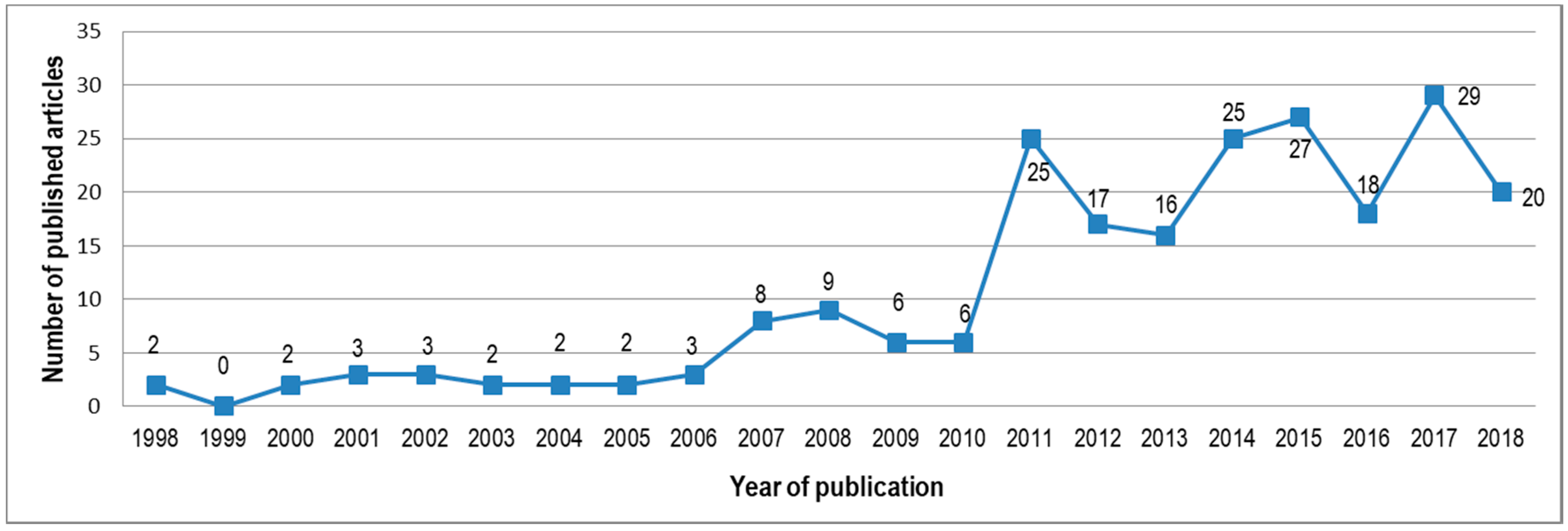
Figure 3.
Classification of articles considering the used keywords.

Figure 4.
The 10 most cited articles based on search in Scopus database.

Figure 5.
Conceptual framework for modelling categories of energy efficiency in supply chain solutions and logistics systems.
Figure 5.
Conceptual framework for modelling categories of energy efficiency in supply chain solutions and logistics systems.
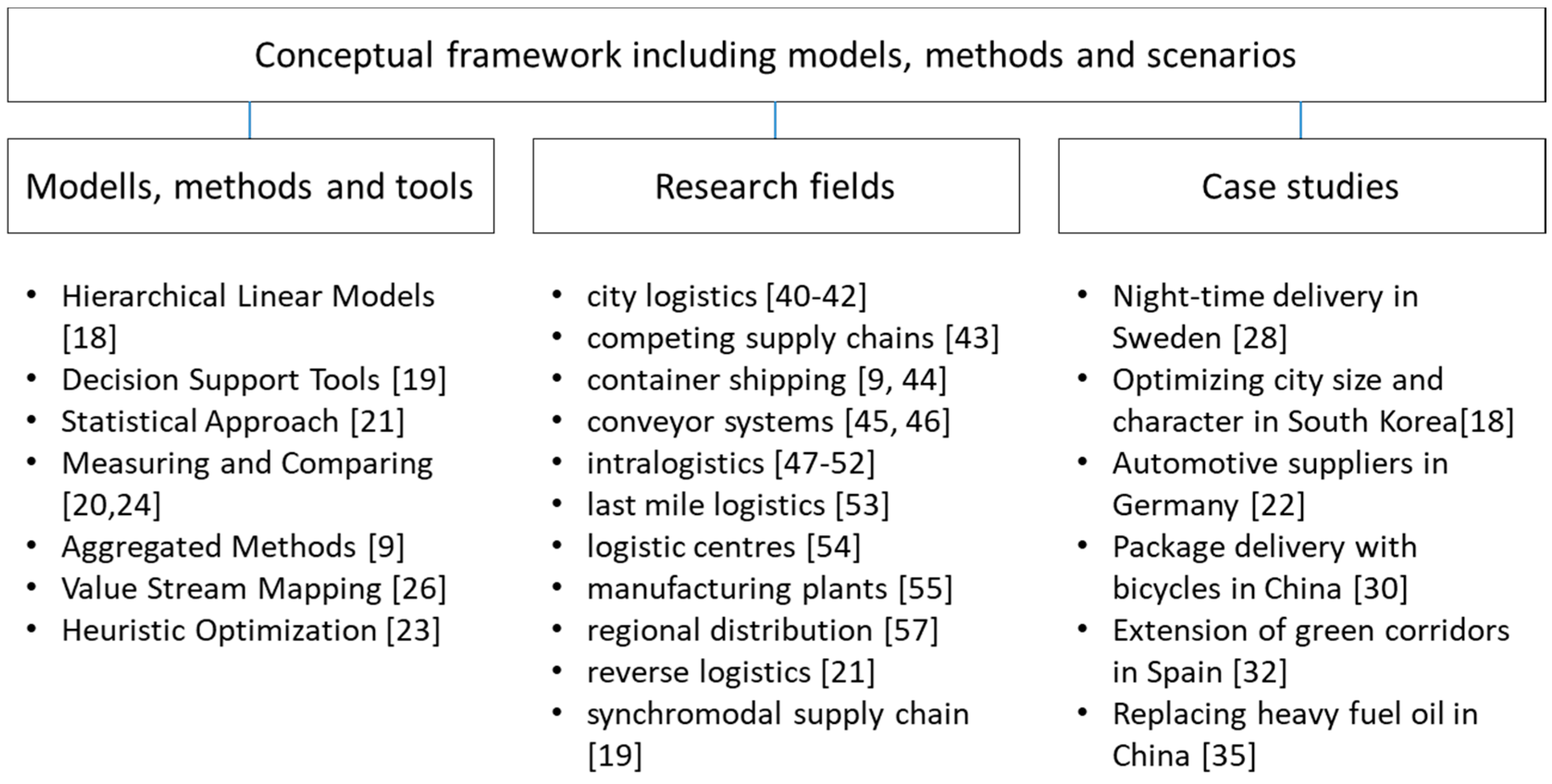
Figure 6.
The model of real-time decision making in last mile logistics to optimize energy efficiency.
Figure 6.
The model of real-time decision making in last mile logistics to optimize energy efficiency.

Figure 7.
The moving behaviour of different particles depending on the distance between particle, event horizon, and photon sphere.
Figure 7.
The moving behaviour of different particles depending on the distance between particle, event horizon, and photon sphere.

Figure 8.
The scheduling of the evaluation of stars inside the Schwarzschild radius influences the convergence speed of the algorithm: (a) If the stars inside the event horizon are not evaluated before absorbed, then the distance between optimal solution inside the event horizon and the black hole should be higher than the distance between the optimal solution and the star; (b) If the star inside the event horizon is evaluated, then the star with a better value of objective function could become the new black hole, while the old black hole becomes a star.
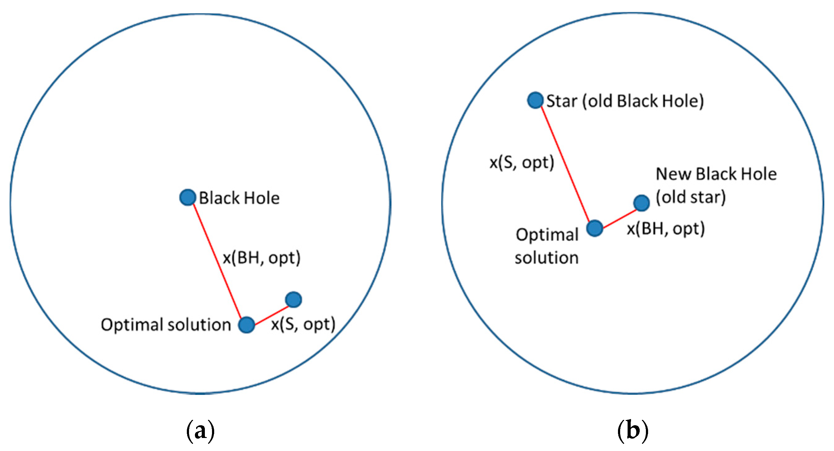
Figure 9.
The permanently decreased Schwarzschild radius prevents the absorption of stars near the event horizon.
Figure 9.
The permanently decreased Schwarzschild radius prevents the absorption of stars near the event horizon.

Figure 10.
After each absorption, a new star is generated around the black hole. The different zones outside the event horizon are represented with different probabilities for the appearance of a new star.
Figure 10.
After each absorption, a new star is generated around the black hole. The different zones outside the event horizon are represented with different probabilities for the appearance of a new star.
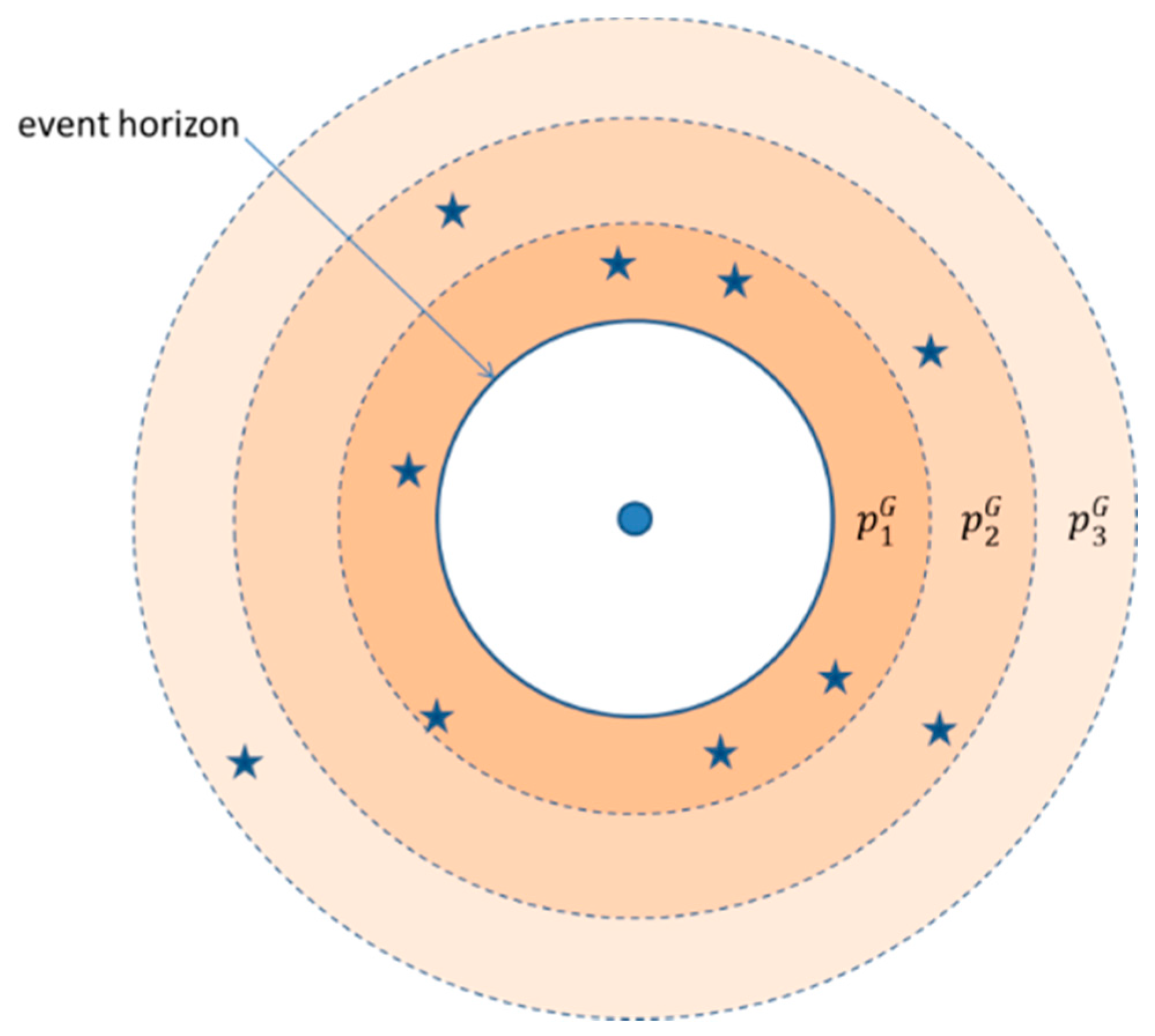
Figure 11.
Loading of delivery trucks with scheduled deliveries. The initial loadings are the loading volumes in the h1 and h2 hubs: 170 pcs, 150 pcs, and 140 pcs. (a) Loading of delivery truck assigned to route 1; (b) Loading of delivery truck assigned to route 2; (c) Loading of delivery truck assigned to route 3.

Figure 12.
Scheduled routes and shuttle services in Scenario 1 and 2: (a) The open tasks are assigned to the parcel delivery service provider (PDSP) receiving the task; (b) The open tasks are assigned to the optimal PDSP.
Figure 12.
Scheduled routes and shuttle services in Scenario 1 and 2: (a) The open tasks are assigned to the parcel delivery service provider (PDSP) receiving the task; (b) The open tasks are assigned to the optimal PDSP.
Figure 13.
Loading of delivery trucks with scheduled deliveries. The initial loadings are the loading volumes in the h1 and h2 hubs: 170 pcs, 150 pcs, and 140 pcs. (a) Loading capacity of delivery truck assigned to route 1 is exceeded after picking up open task 1; (b) Loading of delivery truck assigned to route 2; (c) Loading capacity of delivery truck assigned to route 3 is exceeded after picking up open task 2.

Figure 14.
Scheduled routes and shuttle services in Scenario 3 and 4: (a) The open tasks are assigned to the scheduled routes real-time, time frame constraints are not taken into consideration; (b) The open tasks are assigned to the scheduled routes real-time with time frame constraints.
Figure 14.
Scheduled routes and shuttle services in Scenario 3 and 4: (a) The open tasks are assigned to the scheduled routes real-time, time frame constraints are not taken into consideration; (b) The open tasks are assigned to the scheduled routes real-time with time frame constraints.
Figure 15.
Loading capacities of delivery trucks after rescheduling. The initial loadings are the loading volumes in the h1 and h2 hubs: 170 pcs; 150 pcs; and 140 pcs. (a) Loading capacity of delivery truck assigned to route 1 after rescheduling; (b) Loading of delivery truck assigned to route 2 after rescheduling; (c) Loading capacity of delivery truck assigned to route 3 after rescheduling.
Figure 16.
Scheduled routes without and with constrained time frame in Scenario 5: (a) The open tasks are assigned to the scheduled routes real-time, time frame constraints are not taken into consideration; (b) The open tasks are assigned to the scheduled routes real-time with time frame constraints.

Figure 17.
Results of rescheduling of open tasks not to exceed constrained time frames.

Figure 18.
Comparison of energy consumption of the solutions in scenarios.


Table 1.
Units of measures used in the model.
| Measure Type | Unit |
|---|---|
| Positions of hubs, delivery points, and open tasks | GPS coordinates |
| Energy usage of package delivery trucks | litre/delivery of all packages |
| Specific energy usage of package delivery trucks | litre/100 km |
| Loading capacity of package delivery trucks | pcs of standard postal boxes |
| Lengths of delivery routes | km |
| Assignment matrices | [0, 1] |
Table 2.
Performance evaluation of different BHA solutions with benchmarking functions.
| Benchmarking Function | BHA | BHA/DSR 1 | BHA/HR 2 | BHA/LS 3 |
| 4.24 × 10−04 | 1.48 × 10−05 | 6.80 × 10−04 | 7.06 × 10−04 | |
| 3.24 × 10−02 | 3.24 × 10−02 | 3.24 × 10−02 | 3.24 × 10−03 | |
| 3.56 × 10−09 | 3.56 × 10−03 | 3.56 × 10−03 | 3.56 × 10−04 | |
| 8.96 × 10−09 | 7.01 × 10−09 | 1.41 × 10−07 | 4.61 × 10−09 | |
| Benchmarking Function | DSR/HR | DSR/LS | LS/HR | DSR/LS/HR |
| 3.59 × 10−05 | 2.54 × 10−04 | 2.54 × 10−04 | 3.70 × 10−05 | |
| 3.24 × 10−02 | 3.24 × 10−02 | 3.24 × 10−02 | 3.24 × 10−02 | |
| 3.56 × 10−03 | 3.56 × 10−03 | 3.56 × 10−03 | 3.56 × 10−04 | |
| 4.45 × 10−09 | 8.18 × 10−09 | 1.55 × 10−08 | 5.52 × 10⁻¹⁰ |
1 Decreased Schwarzschild radius, 2 Hawking radiation, 3 Lucky star.
Table 3.
Time frame parameters and package volumes of scheduled deliveries of the scenarios.
| PDSP 1/Route/Destination | Scheduled Delivery | Lower Limit of Delivery Time | Upper Limit of Delivery Time | Loading 2 |
|---|---|---|---|---|
| 1.1.1 | 10:00 | 9:00 | 10:10 | 20 |
| 1.1.2 | 11:00 | 11:00 | 11:05 | −30 |
| 1.1.3 | 12:00 | 11:00 | 12:45 | −40 |
| 1.1.4 | 12:30 | 12:00 | 14:00 | 15 |
| 1.1.5 | 14:00 | 12:00 | 16:00 | 10 |
| 1.2.1 | 10:20 | 9:00 | 10:30 | 30 |
| 1.2.2 | 10:45 | 10:00 | 12:00 | −40 |
| 1.2.3 | 11:50 | 11:00 | 13:00 | −50 |
| 1.2.4 | 12:30 | 12:00 | 14:00 | −10 |
| 1.2.5 | 13:30 | 12:00 | 16:00 | 20 |
| 1.2.6 | 14:00 | 12:00 | 14:00 | −55 |
| 2.1.1 | 10:20 | 9:00 | 11:00 | 20 |
| 2.1.2 | 10:45 | 10:00 | 11:40 | −10 |
| 2.1.3 | 11:50 | 11:00 | 12:55 | 30 |
| 2.1.4 | 12:10 | 12:00 | 14:00 | 20 |
| 2.1.5 | 12:40 | 12:00 | 16:00 | −10 |
| 2.1.6 | 13:15 | 12:00 | 15:30 | −25 |
1 Package Delivery Service Provider, 2 Positive loading refers to pickup, while negative loading to delivery.
Table 4.
Time frame parameters and package volumes of open tasks of the scenarios.
| Open Task | PDSP Receiving the Open Task Assignment | Loading | Pickup Time | Delivery Time | ||
|---|---|---|---|---|---|---|
| Lower Limit | Upper Limit | Lower Limit | Upper Limit | |||
| 1 | 2 | 35 | 10:00 | 12:00 | 12:00 | 14:00 |
| 2 | 1 | 40 | 9:00 | 11:00 | 13:00 | 14:15 |
© 2018 by the author. Licensee MDPI, Basel, Switzerland. This article is an open access article distributed under the terms and conditions of the Creative Commons Attribution (CC BY) license (http://creativecommons.org/licenses/by/4.0/).
Share and Cite
MDPI and ACS Style
Bányai, T. Real-Time Decision Making in First Mile and Last Mile Logistics: How Smart Scheduling Affects Energy Efficiency of Hyperconnected Supply Chain Solutions. Energies 2018, 11, 1833. https://doi.org/10.3390/en11071833
AMA Style
Bányai T. Real-Time Decision Making in First Mile and Last Mile Logistics: How Smart Scheduling Affects Energy Efficiency of Hyperconnected Supply Chain Solutions. Energies. 2018; 11(7):1833. https://doi.org/10.3390/en11071833
Chicago/Turabian StyleBányai, Tamás. 2018. "Real-Time Decision Making in First Mile and Last Mile Logistics: How Smart Scheduling Affects Energy Efficiency of Hyperconnected Supply Chain Solutions" Energies 11, no. 7: 1833. https://doi.org/10.3390/en11071833
Note that from the first issue of 2016, this journal uses article numbers instead of page numbers. See further details here.