A Novel Hierarchical Control Strategy for Low-Voltage Islanded Microgrids Based on the Concept of Cyber Physical System


Institute of Electrical Engineering, Yanshan University, Qinhuangdao 066004, China
*
Authors to whom correspondence should be addressed.
Energies 2018, 11(7), 1835; https://doi.org/10.3390/en11071835
Submission received: 24 May 2018
/
Revised: 6 July 2018
/
Accepted: 10 July 2018
/
Published: 12 July 2018
(This article belongs to the Section F: Electrical Engineering)
Abstract
:Based on the concept of cyber physical system (CPS), a novel hierarchical control strategy for islanded microgrids is proposed in this paper. The control structure consists of physical and cyber layers. It’s used to improve the control effect on the output voltages and frequency by droop control of distributed energy resources (DERs), share the reactive power among DERs more reasonably and solve the problem of circumfluence in microgrids. The specific designs are as follows: to improve the control effect on voltages and frequency of DERs, an event-trigger mechanism is designed in the physical layer. When the trigger conditions in the mechanism aren’t met, only the droop control (i.e., primary control) is used in the controlled system. Otherwise, a virtual leader-following consensus control method is used in the cyber layer to accomplish the secondary control on DERs; to share the reactive power reasonably, a method of double virtual impedance is designed in the physical layer to adjust the output reactive power of DERs; to suppress circumfluence, a method combined with consensus control without leader and sliding mode control (SMC) is used in the cyber layer. Finally, the effectiveness of the proposed hierarchical control strategy is confirmed by simulation results.
1. Introduction
With the deterioration of the global environment and the shortage of energy, the distributed generation technologies using clean and renewable energy in power system have been used widely [1,2]. Currently, the distributed energy resources (DERs) include photovoltaic, wind turbine, micro turbines, fuel cells, etc. In general, these energy resources can provide energy for the normal operation of the load. However, after these sources are connected to the main grid, DERs acquire quasi-load characteristics. IEEE 1547 has set rules of the connection standard between DERs and large power systems. It requires operation withdrawal of each DER when a fault occurs in the large power system. This has greatly limited of full deployment of DERs. For the sake of coordinating the conflict between the main grid and DERs, fully exploiting the potential of DERs and promoting larger scale of application of DER technology, the notion of “micro-grid” has been advocated [3,4]. There are two kinds of operation modes that can be applied in a micro-grid. These modes include the grid-connected mode and the islanded mode [5,6]. In grid-connected mode, the micro-grid can absorb (inject) power from (into) the main-grid. Meanwhile, the voltages and the frequency of DERs are determined by the main grid. When the main grid fails, the microgrid will be disconnected from the main grid. At this time, the microgrid will be turned into the islanded operation mode. In this mode, the microgrid needs to maintain the stability of voltage and frequency through its own corresponding control, and to support a stable energy for the load. Therefore, the efficient strategies must be studied to control the DERs in islanded microgrid.
Recently, a majority of DERs are connected to micro-grids through inverters, so the control strategies of inverters are of great importance. In islanded mode, the droop control strategy is generally used to control the DER inverters. However, this control strategy is obtained by approximation, so the output voltages and frequencies of the controlled DERs cannot reach the reference values. Moreover, each source corresponds to different transmission line impedance, so the reactive power cannot be allocated properly. Therefore, studies on improved control methods for inverters have received extensive attention, such as a decentralized controller proposed in [7] to coordinate the reactive power injections of photovoltaic (PV) generators in order to accomplish the voltage regulation in distribution networks. This method reduces the computational burden of centralized voltage controller, making the research of great practical significance. However, a decentralized control strategy can’t coordinate all DERs within the microgrid in an optimal way due to lack of broader available communication data. An improved self-adaptive droop control method was proposed in [8]. To deal with different external disturbances, the voltage and frequency in this method could be adjusted automatically. Based on the design of virtual impedance and virtual power source, a novel droop control method was designed in [9]. This method can achieve power decoupling and enable droop control to be used. But it is not convenient to use this method in the practical power system. An improved droop control strategy by using the virtual power was proposed in [10], the power decoupling could be also achieved by this strategy. However, there are still errors between the controlled values and the reference values by using the control methods proposed in [8,9,10].
Reactive power control is also a key issue in microgrid research. At present, a lot of literature has studied the reactive power control of DER in distribution networks, such as a centralized nonlinear auto-adaptive controller proposed in [11] to adjust the voltage in controlled system by adjusting the reactive power supplied by photovoltaic. A decentralized nonlinear auto-adaptive controller is proposed in [12] for reducing system losses by the optimal management of the reactive power supplied by the inverters of PV units. However, these two papers do not solve the power allocation problem in DERs. In order to solve this problem, many scholars put forward the corresponding improved control method. For example, a networked-based distributed power sharing method is proposed in [13] to realize the proportional distribution of load in islanded microgrids. However, the problem of communication disturbance had not been solved in this article. In [14], a distributed control strategy was proposed, which could improve the voltage control effect and ensured the reasonable distribution of power in the low-voltage microgrid at the same time. However, the proposed method is difficult to implement at present.
The problem of circumfluence is also a key issue in the study of how to keep the microgrid stable. Circumfluence often occurs at the common nodes of parallel DERs. The problem is caused by the voltage differences of parallel DERs and/or the differences of transmission line impedances. The appearance of circumfluence reduces the performance of the parallel system, which will cause the inverter to stop working and may result in serious consequences. Certainly, there are some studies aimed at solving this problem: In [15], an inverter control method which can suppress harmonic and circumfluence is designed in an islanded microgrid, but the design process is complicated. There are few literatures using communication data to suppress the circumfluence.
With the concept of cyber physical system (CPS) and “smart grid” has been put forward, the concept of CPS is more and more extensive used in power system [16,17]. Because the micro-grid is an important component of “smart grid”, the application of CPS in micro-grid has been also studied in recent years. Meanwhile, the concept of hierarchical control by using communication data to solve physical problems has been also proposed. The control strategies of inverters can be mainly divided into centralized control and decentralized control methods [18]. In the centralized control, all controllers are under unified management by a central controller, so this method is dependent on the reliable communication. Nevertheless, it is difficult to guarantee the stability of the complex CPS. The decentralized control method can achieve the “plug-and-play” for DERs. Under this method, each DER is controlled by local controller without a communication network. However, the system voltage may not be ensured effectively due to the lack of coordination among DERs. Therefore, the strategy of distributed secondary control based on the principle of consensus control is generally used to improve the control effect on DERs. There are some typical related studies. By using the consensus algorithm and communication data, improved control strategies for the frequencies of DERs were proposed in [19,20]. Based on the consensus theory and the communication network, a secondary control strategy was proposed in [21,22,23]. The control effect on voltages and frequencies of DERs had been all improved by using the secondary controller. However, the parameters of the controllers proposed in [19,23] are complicated to select, so it’s not convenient to design the proposed secondary controllers as described in these two papers. Furthermore, with the added secondary control in the microgrid, the cost of using a communication network is also increased. How to use the communication network more reasonably to design the secondary controller is a practical problem.
In order to improve the control effect of DERs and suppress the circumfluence, a novel hierarchical control strategy is proposed in this paper. Based on the concept of CPS, the hierarchical control is divided into the cyber layer and the physical layer. The original contributions of the proposed control method are given as follows:
- (1)
- Design an event-triggered secondary control strategy to control the output voltage and frequency of each DER. The event-trigger mechanism is designed in physical layer at first. When the trigger conditions in mechanism are not met, only the droop control (i.e., the primary control) is used to control the voltage and frequency. Otherwise, a virtual leader-following consensus control method will be designed in cyber layer to accomplish the secondary control on DERs.
- (2)
- Design the method of double virtual impedance in physical layer to decouple the system and share the reactive power among DERs reasonably (i.e., share the reactive power among DERs according to the capacity ration of DERs). The first virtual impedance is used to ensure the output voltage which through the DER’s output impedance and the first virtual impedance to be the same value. The second virtual impedance is used to decouple the control system in dq coordinate system (to make sure the droop control can be applied in a low-voltage microgrid) and share the reactive power of DERs proportionally.
- (3)
- Design the method combined with sliding mode control (SMC) and the consensus control without leader to suppress circumfluence. The specific design process is as below: first, Kirchhoff’s voltage law and Kirchhoff’s current law are used to construct the model of the physical layer. Then, the SMC is used to eliminate the disturbance caused by double virtual impedance and parameter perturbation. Afterwards, the consensus control method is used to design the coordinate controller. Finally, the effectiveness of the proposed controller is proved by using Lyapunov theory, and the circumfluence can be suppressed by using this controller.
This paper is organized as follows: the novel hierarchical control structure of micro-grid is established in Section 2. In Section 3, the secondary control strategy of DER is proposed in detail. In Section 4, the double virtual impedance for DERs is designed. In Section 5, the SMC and coordinated controller is designed to suppress circumfluence. The corresponding simulation studies are provided in Section 6. The overall conclusions of the paper are collected in Section 7.
2. The Design of the Hierarchical Control Strategy
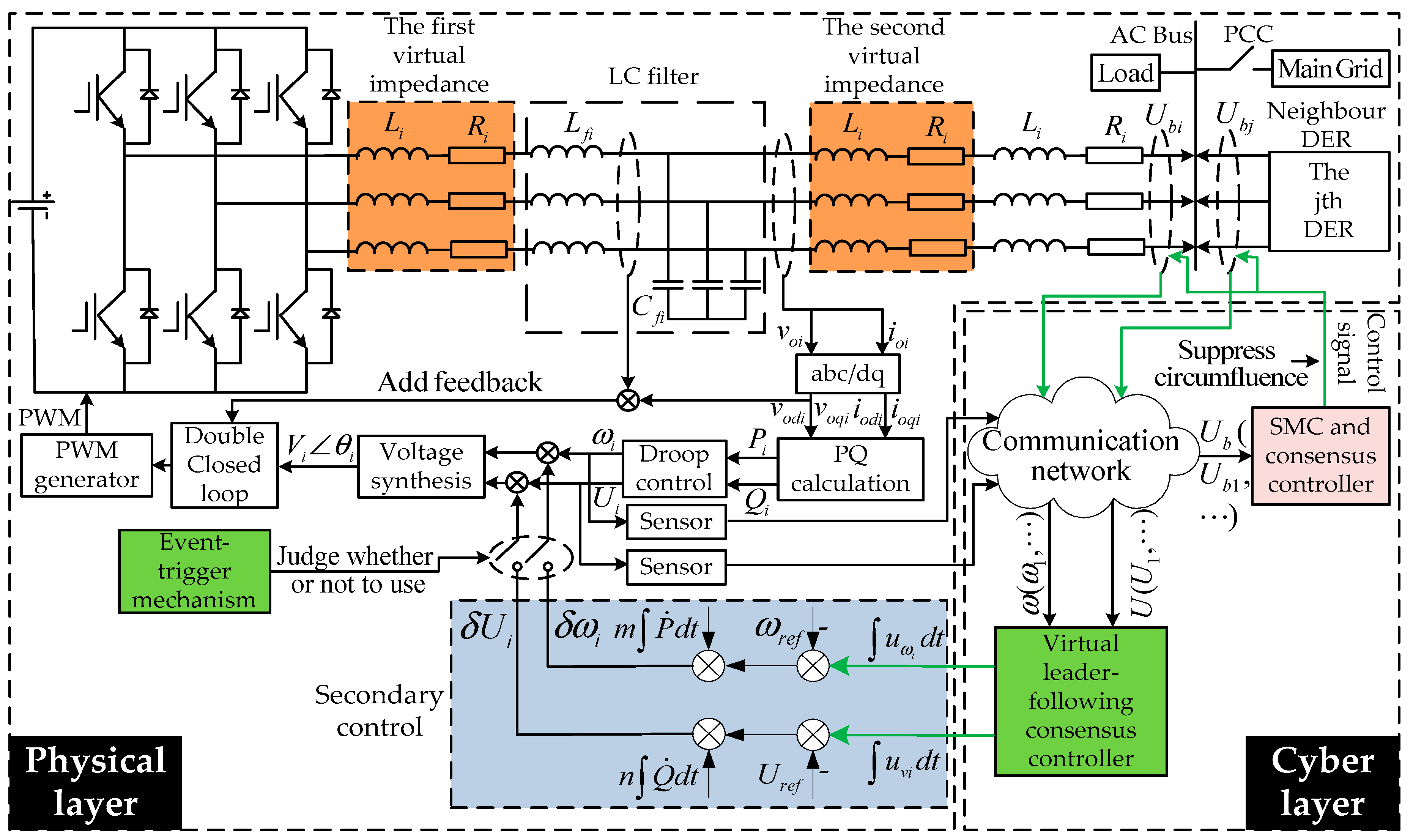
In the past, hierarchical control often refers to two levels of control: secondary control and primary control, but in this paper, according to the concept of CPS (the CPS consists of the communication system and the physical system. It is a complex system which includes the computing part, communication network and physical entities [24]), the hierarchical control refers to the cyber layer and physical layer. The communication data in the cyber layer is not only used to accomplish the secondary control, but also to suppress the circulation. It is our innovation to combine the concepts of CPS and hierarchical control into the control structure of an islanded microgrid at the same time. In this paper, the related data of neighbor DERs is needed to design the distributed coordinated secondary controller for each DER. This caters to the concept of CPS. Meanwhile, if the secondary control is designed without the relevant data of neighbor DER, the effect of cooperative control cannot be accomplished. This will lead to the control process of each DER being out of sync, so based on the concept of CPS, the hierarchical control structure of the i-th DER is constructed as shown in Figure 1.
The control structure of each DER consists of the physical layer and the cyber layer. In the physical layer, all DERs in the microgrid are connected by an AC-bus (alternating current bus). Through the bus, the DERs can be connected to drive the load operation. In Figure 1, many parts (e.g., inverter and double impedances, etc.) of the neighbor DER have been omitted. The specific structures of the omitted parts are similar to that of the corresponding parts of the i-th DER. In the cyber layer, each DER is connected to the neighbour DERs by sensors. All the DERs and sensors constitute the communications network. For the i-th DER, the output voltage and frequency of the neighbour DER will be transmitted to the i-th consensus controller through the sensor at first. Then, the consensus control will be accomplished by using the consensus controller.
There is a consensus controller, virtual leader-following consensus controller and communication network in the cyber layer. In the physical layer, there are a PQ (active power and reactive power) calculation part, droop controller, voltage synthesis part, secondary control part, event-trigger mechanism, double virtual impedance and double closed loop (including voltage loop and current loop), etc. Each DER can be regarded as an agent which has two functions: “consistency calculation” and “data communication”, so the secondary control can be accomplished by using the communication data in the cyber layer. The roles of the components and the control process of secondary control are explained as follows: At first, the output data (e.g., voltage) of the i-th DER and the neighbour DERs are controlled by droop control (primary control). Then, the output voltage data and frequency data of the droop control will be transmitted to the communication network as the communication data. Each controlled DER has a virtual leader-following consensus controller. The consensus controller is used to accomplish the virtual leader-following consensus control. Meanwhile, the secondary control on voltage and frequency will be accomplished by adding feedback values. The feedback values are obtained by using the virtual leader-following consensus control. Afterwards, the obtained voltage and frequency will be transmitted to the voltage synthesis part. The voltage synthesized by this part will be transmitted to the double closed loop. In this double closed loop, the output of the voltage loop will be set as the reference values of the current loop. At last, the output of the current loop will be used to generate the pulse-width modulation (PWM) signal to control the operation of DER through the inverter. The direct current (DC)-link output from the DER will be converted into AC-link through inverter. The output AC-link of the inverter will flow through the double virtual impedance and line impedance, thus driving the load operation.
In the control process, “consistency calculation” refers to the ability to accomplish the corresponding consensus control by designing the consensus controller. Consistency control is accomplished by iterative computation, so the corresponding ability is called as “consistent calculation”; “voltage synthesis” refers to the synthesis of a voltage vector by voltage amplitude and phase angle output from droop control and secondary control; “PQ calculation” refers to calculating the output active and reactive power of DER by using voltage and current of line impedance; voltage and current double closed loop is a kind of control strategy in PWM rectifier, the purpose of the double closed loop is to realize constant voltage control and constant current control.
In order to suppress the circumfluence among DERs, a method combined with consensus control without leader and SMC is proposed in this paper. The SMC is used to eliminate disturbance at first, and then the consensus controller is used to adjust the output node injection voltage from each DER to the same value. The control signals can be obtained by using the error between the voltage of the controlled DER and its neighbour DER.
3. The Design of the Secondary Controller
3.1. The Design of the Event-Trigger Mechanism on Voltage
In the past, the secondary control is directly added to the islanded microgrid system, which will cause communication loss, but actually, droop control has a certain control effect. The data obtained from droop control can be directly used in the voltage synthesis part to a certain extent, and then accomplish the subsequent control. Therefore, in order to make better use of the secondary control method, an event-triggered secondary control strategy is proposed in this paper. Only when the effectiveness of droop control is not ideal (meet the trigger conditions), the secondary control is adopted. This can effectively reduce the loss of the communication network. The specific design process is as the follows. For the i-th DER, the equation of droop control is shown as below:
where and are the active power and reactive power respectively; and are the droop coefficients; and are the frequency reference value and the voltage reference value respectively. Meanwhile, it can be found that droop control produces errors between the output values and the reference values.
First of all, a voltage deviation index must be constructed in this mechanism to evaluate whether the secondary controller is operating. In this paper, this index is constructed based on the deviation between the actual output reactive power and the ideal output value (the so-called “ideal output value” refers to the allocated value according to the output power capacity ratio of each controlled DER) of the DER. The specific design process is as follows: how much reactive power of each DER needs to output is determined by the total reactive power demand and the proportion of this DER in it. Define there are n DERs, and the output reactive power of the i-th DER can be expressed as below:
where (), and are the coefficients; is the demand for total reactive power; is the ideal output reactive power.
For the i-th DER, it is defined that the deviation between the actual output reactive power and the ideal output value should not exceed the percent of the maximum reactive power. For the i-th DER, the floating range of output power allowed by the system is:
where and are the reactive power of actual output and maximum reactive power of allowable output of the i-th DER, respectively.
Take Equations (2) and (3) into Equation (1), and the allowable range of output voltage for the i-th DER is as below:
and there are:
where and are the upper and lower bounds of the allowable range.
The specific event-trigger mechanism is shown in Figure 2.
As shown in Figure 2, the primary control strategy (droop control) is used to control the output voltage of the i-th DER when the change of voltage is within the allowable range. When the floating range of the output voltage exceeds the allowable range, the secondary control strategy will be implemented to maintain the stability of the output voltage.
It’s similar to the design process of event-trigger mechanism on voltage, the event-trigger mechanism on frequency can be also obtained (omit it in this paper to avoid repeating). And the range which is from to is marked as the scope of the allowable range for frequency deviation.
3.2. The Design of the Secondary Control on Voltage
Based on the Equation (1), the amplitude of the output voltage can be expressed in the dq coordinate system as below:
Therefore, the droop control on voltage can also be written as the following equation:
The goal of secondary control on voltage is to design the appropriate control method to adjust to . Based on the differential of Equation (8) and set as an auxiliary variable, there is:
In fact, each DER in the microgrid system can be regarded as an agent. Each one can transmit its state to other DERs and receive the state of others. If each DER is treated as a follower and the corresponding state of leader is set to a reference value, the secondary control can be achieved through the leader-following consensus theory (see Appendix A). The corresponding consensus controller can be designed as below:
where and represent the voltage of the i-th DER and the j-th DER respectively; is the voltage of the virtual leader; is the gain in the protocol. The feedback on voltage is as below:
Based on the differential of Equation (1) and set an auxiliary variable in this subsection, there is:
Similar to the consensus controller on voltage, the consensus controller on frequency can be designed as below:
where and are the frequency of the i-th DER and the j-th DER respectively; is the voltage of the virtual leader; is the gain in the protocol. The feedback on frequency can be designed as below:
Remark 1.
The premise of leader-following consensus control is to ensure the existence of a directed spanning tree in the communication network. In the directed tree, to make the leader as the source node and contain the entire controlled DER, it is necessary to ensure that the leader can deliver the data to the controlled DER (i.e., keep contact to any controlled DER). But in the actual power system, it’s not convenient to select a leader in the power system. So, a virtual leader is used in this paper. The so-called “virtual leader” means that the values of and are set in advance (fixed value) in the consensus controller corresponding to each DER. This ensures the completion of the leader-following consensus control. But there is no real leader, so it’s called “virtual leader”. In this strategy, the state of each controlled DER in the network will be consistent to the corresponding state of virtual leader eventually.
4. The Design of the Method of Double Virtual Impedance
The structure in Figure 3 is set as the example to explain the method of designing the double virtual impedance.
In the figure above: and are the output voltages of the i-th DER and the j-th DER, respectively; and are the output voltages through the DER’s equivalent output impedance and the first virtual impedance; and are the currents of the i-th DER and the j-th DER, respectively; is the voltage of the load; and are the outputs impedance voltages of the i-th DER and the j-th DER respectively; and are the first virtual impedance designed; and are the designed second virtual impedance; and are line impedance; is the load impedance.
1. The design of the first virtual impedance:
The first virtual impedance is used to ensure that and can be modified as the same value. Take the structure in Figure 3 as the example, there are:
so, the first virtual impedance can be obtained by solving the solution of the Equation (15).
2. The design of the second virtual impedance:
In this paper, the control system in dq coordinate system can be decoupled by adding the second virtual impedance. In addition, the reactive power of each DER can also be shared proportionally by using this virtual impedance.
The droop control of the i-th DER is shown as Equation (1). It is only applicable to the case of high inductance of the line impedance, but in fact, the microgrid is usually as the low-voltage power grid, so the lines of microgrids usually have a large resistance. To solve this problem, the second virtual impedance is designed as a negative value. By using the negative virtual reactance to counteract with the line reactance, thus achieving the purpose of power decoupling [8], so there is:
Meanwhile, for the i-th DER, the drop of voltage on this virtual impedance and line impedance can be expressed as below [25]:
As the structure shown in Figure 3, there is:
Remark 2.
When is small, it can be considered that .
Taking Equation (19) into Equation (1), there is the following equation can be obtained:
To share the reactive power among DERs according to the capacity ration of DERs, the second virtual inductor must meet the following condition:
If Equation (21) is met, the output voltage from droop control of the two DERs can be adjusted to the same value. We have:
Based on the above analysis, the Equations (15), (16) and (21) must be met for designing the double virtual impedance.
5. The Design of the Coordinated Controller to Suppress Circumfluence
The circumfluence usually exists in the common connected node of the parallel DERs and it will affect the stable operation of the microgrid. The circumfluence refers to the phenomenon that the current flows from the high voltage source to the low voltage source because the injected node voltage by each DER is not equal, so the problem of suppressing circumfluence can be viewed as a synchronization problem of node injection voltage. In this subsection, if the node-injected voltage is set as the communication data in this section, the consensus control method without leader can be used to design the coordinated controller, so the control signals can be calculated by using the error between the node-injected voltage of the local DER and the neighbor DER.
5.1. Construct the Circuit Model of Connected Distributed Energy Resources (DERs)
Without losing of generality, the structure in Figure 4 is taken as the example to construct the circuit model of connected DERs. The load in Figure 4 includes resistive load, inductive load and capacitive load.
After applying Kirchhoff’s voltage law and Kirchhoff’s current law to the electrical structure in Figure 4, we have:
where and represent the output voltage of the two DERs through the inverters, respectively; and represent the output connected node voltage of the two DERs respectively. The subscript represent the d-axis or the q-axis components, and the definitions of other variables are similar to that; , and are line impedance; and represent the current flowing through the line impedance; and are resistive loads; and are inductive loads; and are capacitive loads.
The system model can be described as below:
where is the matrix of state variables, is the input matrix, is the output matrix of the system. All matrices in Equation (27) are given in the following matrices.
5.2. The Design of Suppressing the Circumfluence
5.2.1. The Design of Sliding Mode Control (SMC)
Due to the parameter perturbation and the addition of double virtual impedance, disturbance data will appear in Equation (24). At present, there are many methods to maintain the stability of the system, such as robust control and SMC. Among them, the SMC has a strong robustness. It is composed of a sliding mode surface and a sliding mode controller. The function of the sliding mode controller is to make the controlled object reach the sliding mode surface and make it stable along the sliding mode surface. Once the controlled object reaches the sliding mode surface, the controlled system will no longer be affected by the external disturbance [26], so the appropriate sliding mode controller is used in this paper to eliminate the disturbance.
The situation that external disturbance occurs in of Equation (24) is set as an example to explain the method of designing SMC. And the disturbance model can be expressed as below:
where is the obtained disturbance data; are parameter perturbations.
For the DER1, the sliding mode controller can be designed as below:
where is the sliding mode controller; and are the components.
And then add Equation (26) into Equation (25), it can be obtained that: .
The sliding mode surface can be designed as below:
where are the coefficients of the sliding mode surface. And there are:
At this point, solve at first. Thus, make , there are:
Afterwards, solve . According to the properties of the sliding mode surface, it is necessary to make . After making and substitute Equation (29) into , there is:
where is a positive constant value. Meanwhile, the control process can be accomplished in the finite time by selecting the approximate parameters. And the time in control process consists two parts: reaching time and sliding time. The reaching time is the required time to make the controlled object reach the sliding surface. Sliding time is the required time for the controlled object to reach stability after reaching the sliding mode surface. The analysis of the two periods of time is as the follows:
Reaching Time
Set a Lyapunov function as , and . The reaching time is set as . After substituting into , there are:
If , there are:
else if , there are:
So, in order to make the controlled system satisfy Lyapunov stability, needs to satisfy .
Sliding Time
The sliding time is set as (, ). And in this stage, there is . When the disturbance is positive, there are:
so, the parameters in the sliding mode surface can be obtained by solving the following optimization problem:
In the same way, the corresponding equations can be obtained when the perturbation is negative.
5.2.2. The Design of Coordinated Controller
The problem of suppressing the circumfluence can be classified as a consistency problem, i.e., the output node injection voltage (controlled state) of each DER is needed to be modified as the same value. The corresponding state error between the i-th DER and the j-th DER is defined as:
where and are the states of the i-th DER and the i-jth DER, respectively. In this paper, the two elements are node injection voltages.
The overall neighbour error is equal to , where , . Set , where is the feedback gain; is the feedback matrix. We have:
so, the dynamic model of the overall controlled system can be shown as below:
Theorem 1.
The system (38) is asymptotically stable, if and only if exists matrix and satisfying the following conditions:
where , represents the maximal singular values, denotes the minimal nonzero singular value. The proof of the theory and the selection of related parameters are given in Appendix B.
6. Simulation Study
In this subsection, the microgrid system shown in Figure 5 is used as the example to carry out the simulation experiment.
In this experimental case, the following settings are used: the three DERs are parallel; the microgrid system is set to operate in the islanded mode; the power capacity ratio of four DERs is set as 4:3:2:1; The original load (Load1) is set as 6 kW/3 kvar. The other specific parameters are shown in Table 1.
6.1. Case1: Verify the Control Effect by the Event-Triggered Secondary Control
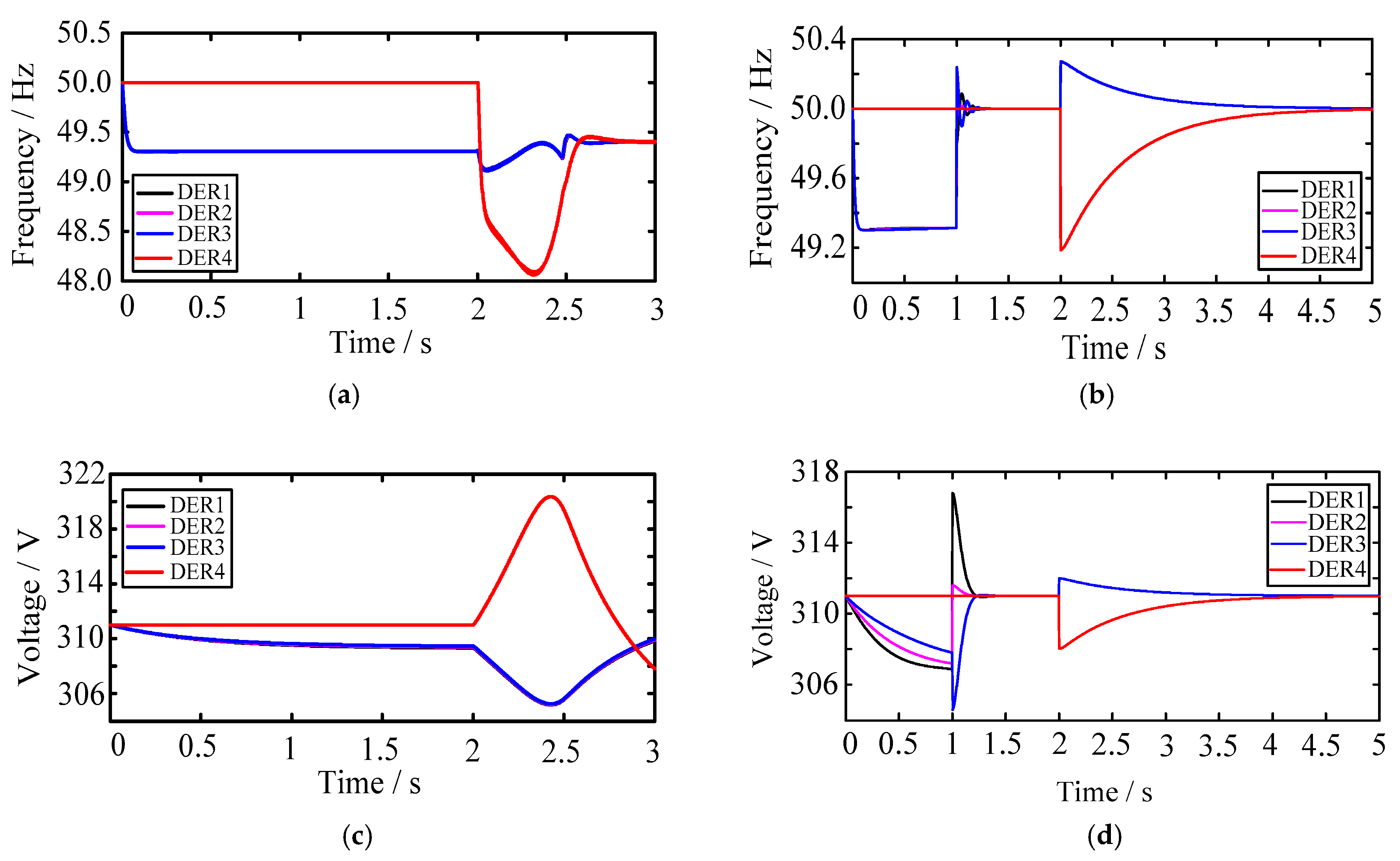
In this experiment, to better reflect the effectiveness of secondary control, the droop control is used as a comparison. Furthermore, to verify the effect of the event-trigger mechanism, there are: In the begin, the range from to is designed from 310 V to 312 V; At t = 1 s, the range from to is designed from 49.5 Hz to 50.5 Hz, so the variation of voltage and frequency should not exceed 1 V and 0.5 Hz, respectively. At the same time, in order to better illustrate the effectiveness of the secondary control strategy, we design four kinds of external disturbances in the control process: (1) Load1 is always running on the system, and the Load2 is added to the system at t = 2 s; (2) The Load1 and Load2 are working at begin. Then, the Load2 is cut off at t = 2 s; (3) The DER4 is added to the system at t = 2 s; (4) The DER4 is working in the system at the beginning. Then, it’s cut off at t = 2 s. The corresponding simulation results are as Figure 6 and Figure 7.
The analysis is as below: As shown in Figure 6a,c, the voltage of the three DERs are among 309.3–309.6 V. After adding Load2 at t = 2 s, the voltage of each DER has dropped. There are errors between the voltages and the corresponding reference value (). The droop control adjusts the frequency to 49.3 Hz. After adding Load2 at t = 2 s, the frequency of each DERs will decline to 49.25 Hz. There are errors between the frequency and the corresponding reference value (). Take the deviation in frequency as the example, the cause of deviation can be explained as follows: The formula for frequency droop control is , so the formula shows that the deviation between and is . Due to and have the following relation: , so will be not equal to , and the deviation is . As shown in Figure 6b,d, the event-trigger mechanism is triggered at t = 1 s. Meanwhile, the secondary control method is also used in the system. At last, the voltage and frequency of every DER are adjusted their respective reference values.
As shown in Figure 7a,c, the voltages of all DERs are among 309.2–309.4 V. When the Load2 is cut off at t = 2 s, the voltages of DERs will be raised. It has errors between the voltages and the corresponding reference value (). The output frequency by droop control is 49.25 Hz. When the Load2 is cut off at t = 2 s, the frequency of DER will be raised to almost 49.3 Hz. There are also errors between the actual value and . By analyzing the variations in Figure 7b,d, it has been found that the controlled values of each DER can be adjusted to their respective reference values by using the secondary control (the trigger conditions are met at t = 1 s). After comparing, it can be found that the control effect of voltages and frequency can be effectively enhanced by the event-triggered secondary control method. In the case of DER changes, the corresponding simulation results are as Figure 8 and Figure 9.
The analysis is as below: In Figure 8a, the droop control adjusts the frequency of DERs to almost 49.3 Hz in steady state. The frequency of DER4 is 50 Hz before it is added in the system. After adding DER4 at t = 2 s, there is a transition between t = 2 s and t = 2.65 s in the control process. Finally, the frequency of the four DERs has been controlled to almost 49.4 Hz. There are errors between the output actual value and . In Figure 8b, the secondary control method is used at t = 1 s. The frequency of each DER will reach 50 Hz at t = 1.3 s (there is a transition between t = 1 s and t = 1.3 s). After adding DER4 at t = 2 s, there is also a transition between t = 2 s and t = 4.5 s. Finally, the frequency of each DER can be adjusted to 50 Hz. In Figure 8c, the droop control makes the voltage tend to almost 309 V. The voltage of DER4 is 311 V before it is added in the system. When the Load2 is added at t = 2 s, the voltages of the first three DERs have dropped. This is because when the DER4 is added at the beginning, the system regards the DER4 as a Load. There is a transition before DER4 works normally in the system. And there are errors between the output actual value and . In Figure 8d, the output voltage of the four DERs by droop control are different before t = 1 s. Meanwhile, the secondary control is added in the system. The voltage of each DER will be adjusted to 311 V at t = 1.3 s (there is a transition between t = 1 s and t = 1.3 s). After adding DER4 at t = 2 s, there is also a transition between t = 2 s and t = 4 s. Finally, the voltage of the four DERs will achieve to 311 V.
In Figure 9a, the frequency of DERs is adjusted by droop control to 49.45 Hz before t = 1 s. When the DER4 is cut off at t = 2 s, the frequency of the first three DERs has drooped to almost 49.3 Hz. There are errors between the output actual value and . In Figure 9b, the secondary control is added in the system at t = 1 s. The frequency of each DER can be adjusted to 50 Hz at t = 1.3 s (there is a transition between t = 1 s and t = 1.3 s). Even if the DER4 is cut off at t = 2 s, it has no obvious effect on frequency. In Figure 9c, the output voltages of DERs by droop control are not consistent and the voltages are between 309.6–309.8 V. After cutting off Load2 at t = 2 s, the voltages of DERs have dropped. There are errors between the output actual value and the reference value. In Figure 9d, the secondary strategy can be added in the system at t = 1 s and the voltages of DERs can be adjusted to 311 V at t = 1.3 s (there is a transition between t = 1 s and t = 1.3 s). There is also no obvious effect on voltage after cutting off DER4 at t = 2 s.
6.2. Case2: Verify the Control Effect on Power Distribution
In this section, the event-triggered secondary control and double virtual impedance has been used first. Meanwhile, the microgrid system is operated in the islanded mode. For verifying the effect of the power distribution by using the double virtual impedance obviously, the load power of Load2 is changed as and (50% of Load1). There are four situations in this simulation: (1) The Load2 is added in the system at t = 2 s; (2) The Load2 is added in the system at begin. It will be cut off at t = 2 s; (3) Add DER4 into the system at t = 2 s; (4) The DER4 is added in the system at the beginning and it will be cut off at t = 2 s. The output active power and reactive power of each DER are shown in Figure 10.
During t = 1 s to t = 2 s, Figure 10a,b show that the output active power and reactive power of DERs can be shared according to the desired ratio of 4:3:2 during the islanded mode. After t = 2 s, the active power and reactive power of DERs are approximately 4 kW/2 kvar, 3 kW/1.5 kvar and 2 kW/1 kvar. This indicates that the active power and reactive power sharing is accurate.
As shown in Figure 10c,d, the Load decreases 50% when t = 2 s. It can be seen that during the micro-grid islanded mode, the output active power and reactive power of DER can be shared according to the desired ratio before t = 2 s. After t = 2 s, the output active power and reactive power of DERs are approximately 1.33 kW/0.67 kvar, 1 kW/0.5 kvar and 0.67 kW/0.33 kvar, which indicates that the active power and reactive power can be shared reasonably by using the novel hierarchical control when Load disturbance occurs in the microgrid system.
When the DER4 is added (or cut off) in the microgrid system, the output active and reactive power of each DER is shown as Figure 11.
The analysis is as below: During t = 1 s to t = 2 s, Figure 11a,b show that the output active power and reactive power of DER1, DER2 and DER3 can be shared according to the desired ratio of 4:3:2 during the islanded mode. After t = 2 s, the DER4 is added to the system. Through a transient process, the output active power and reactive power of four DERs are approximately 2.4 kW/1.2 kvar, 1.8 kW/0.9 kvar, 0.8 kW/0.4 kvar and 0.4 kW/0.2 kvar. It indicates that the active power and reactive power can be allocated in proportion to the capacity of DERs. As shown in Figure 11c,d, under the action of double virtual impedance, four DERs can output power according to capacity ratio before t = 2 s. When t = 2 s, the DER4 is cut off and the output active power and reactive power of DER1, DER2 and DER3 are approximately 2.7 kW/1.38 kvar, 2 kW/1 kvar and 1.33 kW/0.67 kvar, which indicate that the active power and reactive power can be shared more reasonably by the novel hierarchical control when Load disturbance occurs in the system.
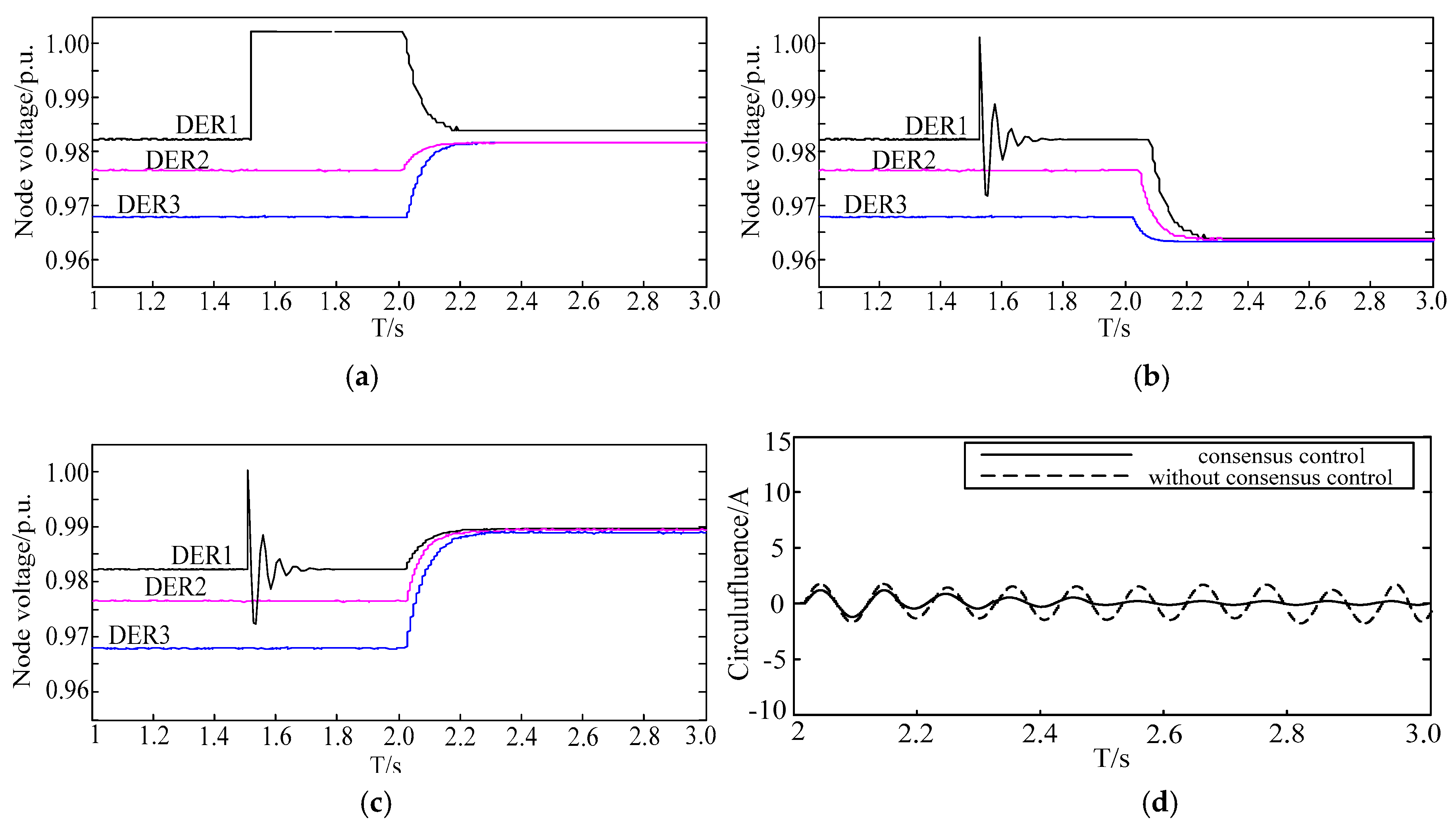
6.3. Case3: Verify the Effect on Supressing Circumfluence
In this case, the connected node of three DERs is set as the study object. The proposed secondary control method and double virtual impedance have been used in the system before t = 1 s. To verify the effect of SMC, we set a step signal in the output data (voltage and frequency) of DER1 as the disturbance data. The amplitude of this signal is set as 3. For sliding mode controller, the time for accomplishing SMC is set as 0.5 s, and the parameters in controller are set as: In order to better illustrate the practicability of the proposed coordinated method, we have designed two situations in this experiment: (1) Add Load2 into the system at t = 2 s; (2) The Load2 is added in the system at begin. It’s cut off at t = 2 s. The simulation results are shown as Figure 12.
In Figure 12a, there are bias in the voltages of three DERs injected into the common node. Meanwhile, the node voltage outputted by DER1 will be greatly overshoot after adding disturbance at t = 0.5 s. Finally, the input node voltage of DER1 is still different from that of the other three DERs. As shown in Figure 12b,c, the disturbance occurs at t = 1.5 s. It can be eliminated in 0.5 s by using the designed SMC. According to the simulation results, regardless of the Load increase or decrease, the designed coordinated controller based on the consistency protocol without leader can ensure the output node voltage of each DER stably. At the same time, the output node voltages of the DERs can be also modified as consistency by using the consensus control method. By comparing with the circumfluence shown in the case without consensus control, it can be seen from Figure 12d that the circumfluence is eliminated obviously through the designed coordinated controller.
7. Conclusions
Based on the concept of CPS, a novel hierarchical control strategy is proposed in this paper. It’s used to improve the control effect of DERs and solve the problem of circumfluence in microgrid. The main contributions of this paper are as below:
- (1)
- An event-triggered secondary control strategy is proposed to improve the control effect on voltages and frequency obtained by droop control of DERs.
- (2)
- A method of double virtual impedance is proposed to share the reactive power according to the capacity ration of DERs in microgrid system.
- (3)
- A method combined with SMC and the consensus control without leader is used to suppress the circumfluence in microgrid system.
Finally, the case1 confirms that the proposed secondary control method can improve the control effect on voltages and frequency obtained by droop control of DERs effectively. The case2 confirms that the output reactive power of each DER can be allocated according to the capacity ration of DERs. It confirms the effectiveness of the proposed double virtual impedance. The case3 confirms that the disturbance caused by virtual impedance and parameter perturbation can be effectively eliminated by the designed SMC. The output node injection voltage from each DER can be adjusted to the same value through the designed coordinated controller. Furthermore, the node circumfluence can be also decreased obviously by using the coordinated controller. Based on the analysis above, the simulation results clearly indicate that the proposed hierarchical control strategy has good performance in terms of validity and stability in islanded microgrids.
Author Contributions
This paper was a collaborative effort among all authors. All authors conceived the methodology, conducted the experiments and wrote the paper.
Acknowledgments
This work is supported by the National Natural Science Foundation of China under Grant 61573303, and Hebei Provincial Natural Science Foundation of China under Grant E2016203092.
Conflicts of Interest
The authors declare no conflict of interest.
Appendix A. Theory Basic
Graph theory: The topology of multi-agent system can be usually represented by a directed graph: . Each agent can be represented as an agent. For a directed graph which consists a set of nodes () and a set of edges (), the n nodes of the directed graph can be seen as n agents. If the i-th node is connected to the j-th node, there should be a line (i.e., communication path) from the i-th node to the j-th node. If any node is connected to any other nodes, the corresponding directed graph is called as “connected strongly”. If there is a directed path which connects all nodes, the corresponding directed path is called as “a directed spanning tree”. The corresponding adjacency matrix of the directed graph can be defined as . If the j-th node is connected to the i-th node, is positive and otherwise. There are no repeated node, i.e., . The degree matrix of is , where . The Laplacian matrix is defined as .
Leader-following consistency theory [27]: In a directed graph (or communication network), it is assumed that there are n agents, and the state of the i-th agent is marked as . If there is only one agent could transfer its state to any other agents along a directed path, the only one agent is called as the leader. The corresponding state of the leader is defined as . The other agents are called as “followers” in the directed graph. For the multi-agent system, the leader–following consistency can be achieved if there is a distributed controller for the i-th agent to make that:
The one order mathematical model can be used to represent the state of each agent. The corresponding equation can be expressed as below:
where is the distributed controller for the i-th agent.
In summary, the state of each agent will be consistent to by a consistency protocol (it’s also called as consensus controller). Without considering the problems of time-delay and topological switching, etc., the consistency protocol is as below [24]:
where represents the relationship between the leader and the i-th agent. If the leader connects to the i-th follower, and otherwise; is the gain in protocol. The state of followers will follow the corresponding state of the leader when using the proper parameters in protocol.
Kronecker product theory: For a matrix , represents the maximal singular value, and represents the minimal nonzero singular value.
Definition A1.
Let. Then the following block matrix is called Kronecker product of and , written .
Appendix B. The Proof of the Theorem 1 Proposed in Section 5
Proof.
The feedback matrix is as below:
Suppose , from Equation (41), we can obtain .
The algebraic Riccati equation is written as:
where . So, can be represented as:
Define the Lyapunov function as , and there are:
The proof is accomplished, so based on Equations (41) and (A1), the coupling gain and the feedback gain matrix can be chosen, respectively, to ensure the asymptotic stability of the controlled system. ☐
References
- Guo, X.; Yang, Y.; Zhu, T. ESI: A novel three-phase inverter with leakage current attenuation for transformerless PV systems. IEEE Trans. Ind. Electron. 2018, 65, 2967–2974. [Google Scholar] [CrossRef]
- Guo, X. A novel CH5 inverter for single-phase transformerless photovoltaic system applications. IEEE Trans. Circuits Syst. 2017, 64, 1197–1201. [Google Scholar] [CrossRef]
- Katiraei, F.; Iravani, M.R. Power management strategies for a microgrid with multiple distributed generation units. IEEE Trans. Power Syst. 2006, 21, 1821–1831. [Google Scholar] [CrossRef]
- Guo, X.; Xu, D.; Guerrero, J.M.; Wu, B. Space vector modulation for DC-link current ripple reduction in back-to-back current-source converters for microgrid applications. IEEE Trans. Ind. Electron. 2015, 62, 6008–6013. [Google Scholar] [CrossRef]
- Elrayyah, A.; Cingoz, F.; Sozer, Y. Construction of Nonlinear Droop Relations to Optimize Islanded Microgrid Operation. IEEE Trans. Ind. Appl. 2015, 50, 3404–3413. [Google Scholar] [CrossRef]
- Guo, X.; Yang, Y.; Wang, X. Advanced control of grid-connected current source converter under unbalanced grid voltage conditions. IEEE Trans. Ind. Electron. 2019. [Google Scholar] [CrossRef]
- Cagnano, A.; Tuglie, E.D. A decentralized voltage controller involving PV generators based on lyapunov theory. Renew. Energy 2016, 86, 664–674. [Google Scholar] [CrossRef]
- Vahidreza, N.; Ali, D.; Frank, L.; Guerrero, J.M. Distributed adaptive droop control for DC distribution systems. IEEE Trans. Energy Convers. 2014, 29, 944–956. [Google Scholar] [CrossRef]
- Dou, C.X.; Zhang, Z.Q.; Yue, D.; Song, M.M. Improved droop control based on virtual impedance and virtual power source in low voltage microgrid. IET-Gener. Transm. Distrib. 2017, 11, 1046–1054. [Google Scholar] [CrossRef]
- Wu, T.; Liu, Z.; Liu, J.; Wang, S.; You, Z. A unified virtual power decoupling method for droop-controlled parallel inverters in microgrids. IEEE Trans. Power Electron. 2016, 31, 5587–5603. [Google Scholar] [CrossRef]
- Cagnano, A.; Tuglie, E.D.; Dicorato, M.; Forte, G.; Trovato, M. PV plants for voltage regulation in distribution networks. In Proceedings of the IEEE Universities Power Engineering Conference, London, UK, 4–7 September 2012; pp. 1–5. [Google Scholar] [CrossRef]
- Cagnano, A.; Tuglie, E.D.; Liserre, M.; Mastromauro, R.A. Online optimal reactive power control strategy of PV inverters. IEEE Trans. Ind. Electron. 2011, 58, 4549–4558. [Google Scholar] [CrossRef]
- Kahrobaeian, A.; Ibrahim, M.A.R. Networked-Based Hybrid Distributed Power Sharing and Control for Islanded Microgrid Systems. IEEE Trans. Power Electron. 2015, 30, 603–617. [Google Scholar] [CrossRef]
- Anand, S.; Fernandes, B.G.; Guerrero, J.M. Distributed control to ensure proportional load sharing and improve voltage regulation in low voltage DC microgrid. IEEE Trans. Power Electron. 2013, 28, 1900–1913. [Google Scholar] [CrossRef]
- Li, Y.; Shi, X.Y.; Fan, X.P. A control strategy for suppressing harmonics and circumfluence in islanded microgrid. In Proceedings of the Chinese Control and Decision Conference, Dalian, China, 26–28 July 2017; pp. 3132–3236. [Google Scholar] [CrossRef]
- Mo, Y.; Kim, T.H.J.; Brancik, K.; Dickinson, D.; Lee, H.; Perrig, A.; Sinopoli, B. Cyber-physical security of a smart grid infrastructure. Proc. IEEE 2012, 100, 195–209. [Google Scholar] [CrossRef]
- Siddharth, S.; Adam, H.; Manimaran, G. Cyber-physical system security for the electric power grid. Proc. IEEE 2012, 100, 210–224. [Google Scholar] [CrossRef]
- Bidram, A.; Davoudi, A. Hierarchical structure of microgrids control system. IEEE Trans. Smart Grid 2012, 3, 1963–1976. [Google Scholar] [CrossRef]
- Liu, W.; Gu, W.; Sheng, W.X.; Meng, X.L.; Wu, Z.J.; Chen, W. Decentralized multi-agent System based cooperative frequency control for autonomous Microgrids with communication constraints. IEEE Trans. Sustain. Energy 2014, 5, 446–456. [Google Scholar] [CrossRef]
- Wang, Z.G.; Wu, W.C.; Zhang, B.M. A fully distributed power dispatch method for fast frequency recovery and minimal generation cost in autonomous microgrids. IEEE Trans. Smart Grid 2016, 7, 19–31. [Google Scholar] [CrossRef]
- Wang, P.B.; Lu, X.N.; Yang, X.; Wang, W.; Xu, D.G. An improved distributed secondary control method for DC microgrids with enhanced dynamic current sharing performance. IEEE Trans. Power Electron. 2016, 31, 6658–6673. [Google Scholar] [CrossRef]
- Bidram, A.; Davoudi, A.; Lewis, F.L.; Qu, Z.H. Secondary control of microgrids based on distributed cooperative control of multi-agent systems. IET-Gener. Transm. Distrib. 2013, 7, 822–831. [Google Scholar] [CrossRef]
- Guo, F.; Wen, C.; Mao, J.; Song, Y.D. Distributed secondary voltage and frequency restoration control of droop-controlled inverter-based microgrids. IEEE Trans. Ind. Electron. 2015, 62, 4355–4364. [Google Scholar] [CrossRef]
- Kim, K.D.; Kumar, P.R. Cyber-Physical systems: A perspective at the centennial. Proc. IEEE 2012, 100, 1287–1308. [Google Scholar] [CrossRef]
- Dou, C.X.; Zhang, B.; Yue, D.; Zhang, Z.Q.; Xu, S.Y.; Hayat, T.; Alsaedi, A. A novel hierarchical control strategy combined with sliding mode control and consensus control for islanded micro-grid. IET-Renew. Power Gener. 2018, 12, 1012–1024. [Google Scholar] [CrossRef]
- You, X.; Hua, C.C.; Peng, D.; Guan, X.P. Leader–following consistency for multi-agent systems subject to actuator saturation with switching topologies and time-varying delays. IET Control Theory Appl. 2016, 10, 144–150. [Google Scholar] [CrossRef]
- Dou, C.X.; Zhang, Z.Q.; Yue, D.; Gao, H.X. An Improved Droop Control Strategy Based on Changeable Reference in Low-Voltage Microgrids. Energies 2017, 10, 1080. [Google Scholar] [CrossRef]
Figure 1.
The hierarchical control structure of the i-th distributed energy resource (DER). AC: alternating current; LC-filter: inductance capacitance filter (i.e., passive filter); PCC: point of common coupling; PQ: active power and reactive power; PWM: pulse-width modulation.
Figure 1.
The hierarchical control structure of the i-th distributed energy resource (DER). AC: alternating current; LC-filter: inductance capacitance filter (i.e., passive filter); PCC: point of common coupling; PQ: active power and reactive power; PWM: pulse-width modulation.

Figure 2.
The proposed event-trigger mechanism on voltage control strategy.
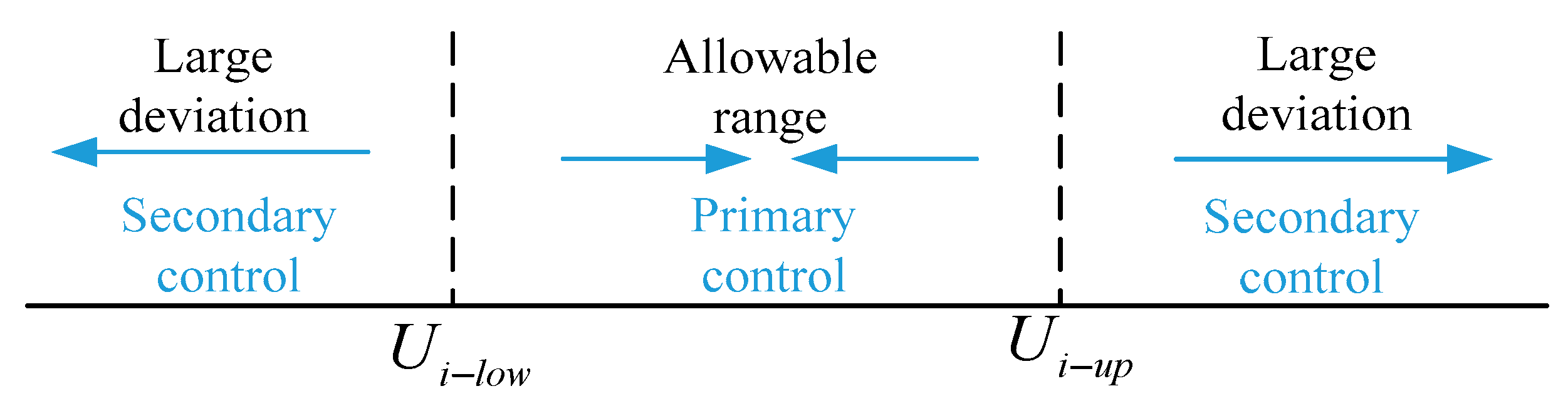
Figure 3.
Topology of two parallel DERs.
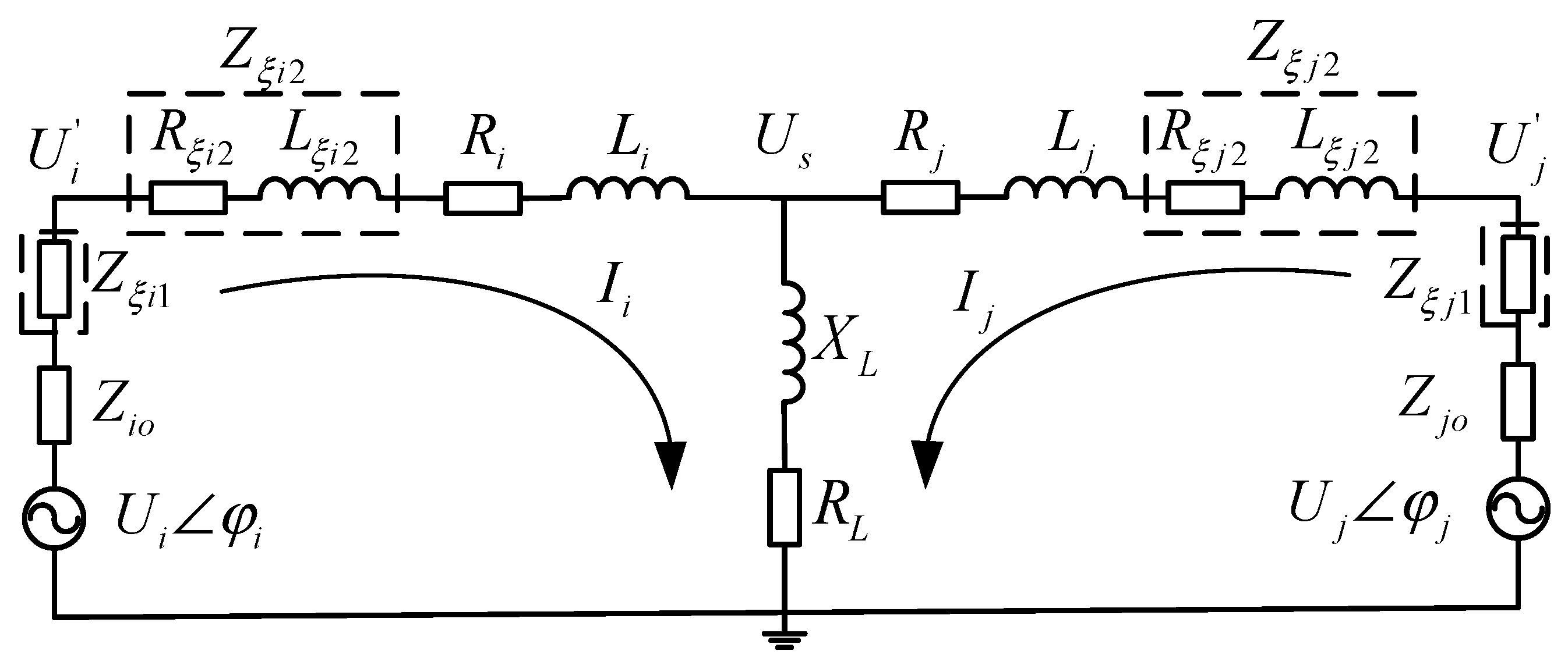
Figure 4.
Circuit model of the connected DERs. R: resistive load; C: capacitive load; L: inductive load.
Figure 4.
Circuit model of the connected DERs. R: resistive load; C: capacitive load; L: inductive load.

Figure 5.
Microgrid system.
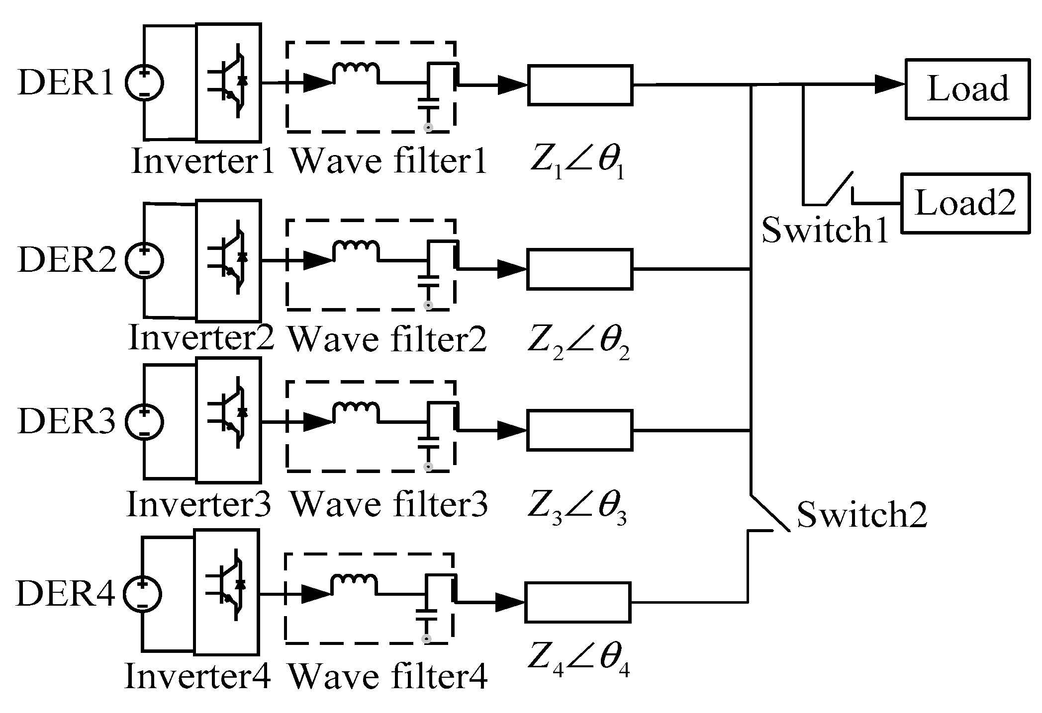
Figure 6.
Variations of DERs when Load2 is added at t = 2 s. (a) Variations of voltage by using traditional droop control; (b) Variations of voltage by using the novel distributed control; (c) Variations of frequency by using traditional droop control; (d) Variations of frequency by using the novel distributed control.
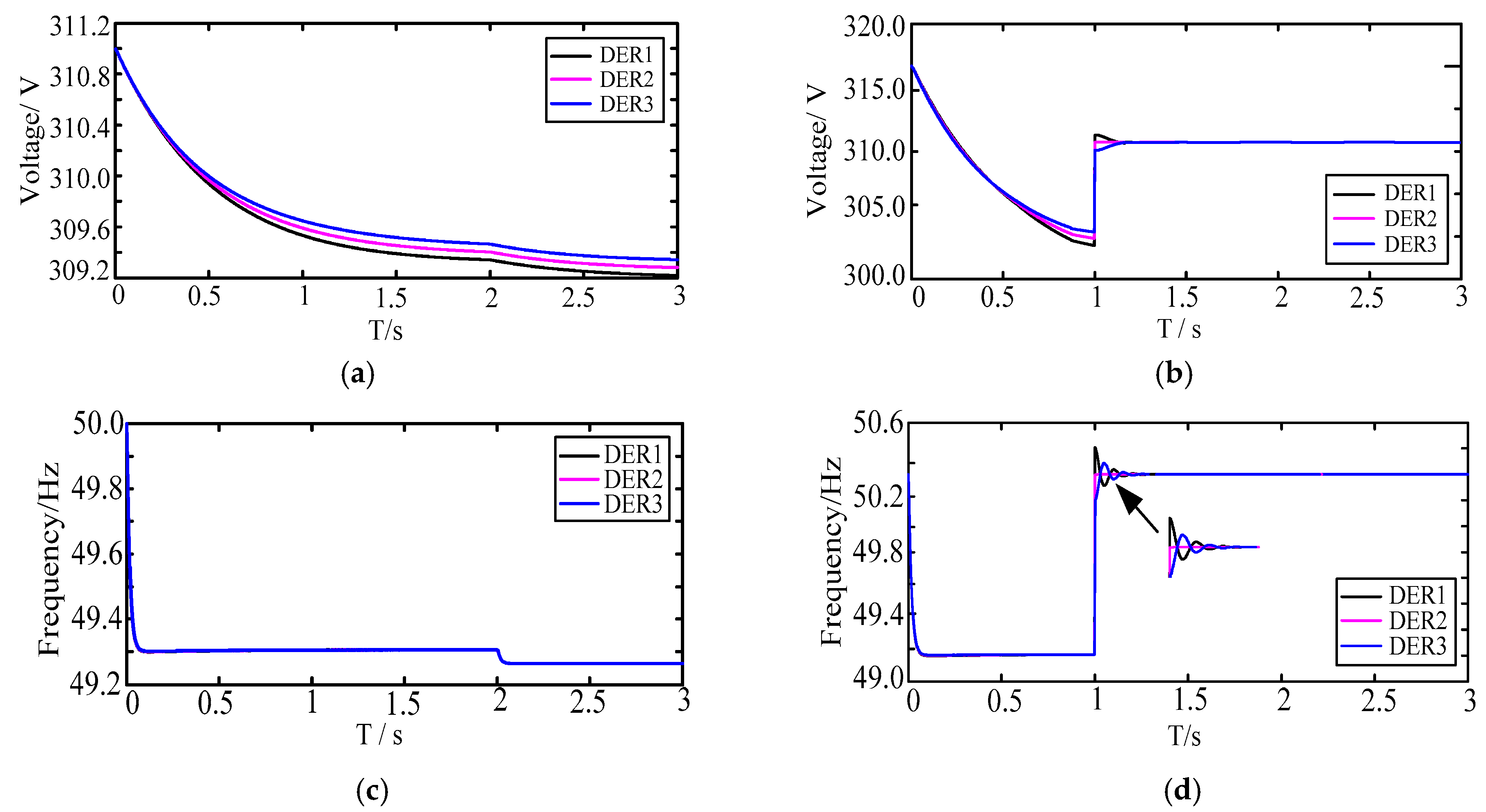
Figure 7.
Variations of DERs when Load2 is cut down at t = 2 s. (a) Variations of voltage by using traditional droop control; (b) Variations of voltage by using the novel distributed control; (c) Variations of frequency by using traditional droop control; (d) Variations of frequency by using the novel distributed control.
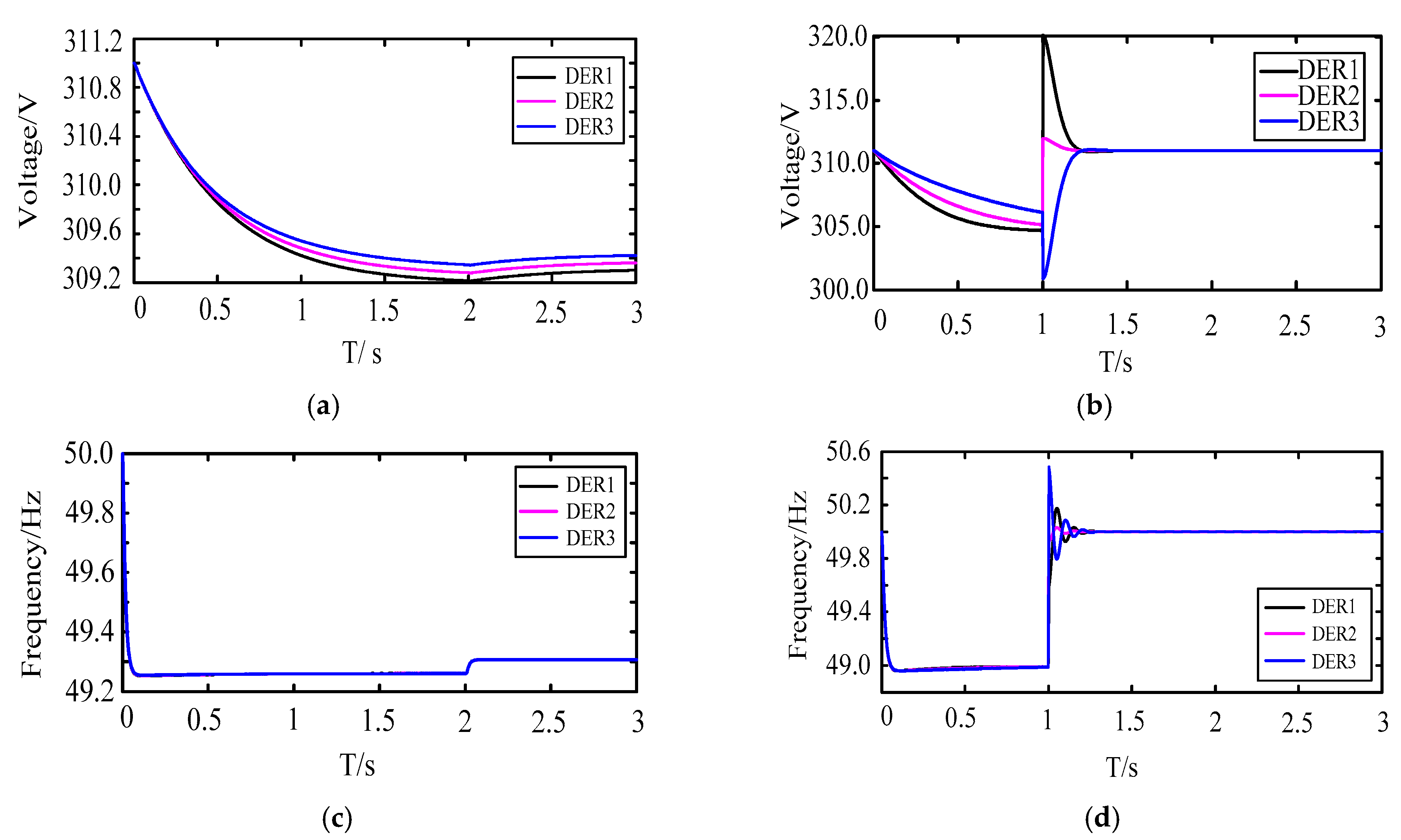
Figure 8.
Variations of DERs when DER4 is added at t = 2 s. (a) Variations of voltage by using traditional droop control; (b) Variations of voltage by using the novel distributed control; (c) Variations of frequency by using traditional droop control; (d) Variations of frequency by using the novel distributed control.

Figure 9.
Variations of DERs when DER4 is cut off at t = 2 s. (a) Variations of voltage by using traditional droop control; (b) Variations of voltage by using the novel distributed control; (c) Variations of frequency by using traditional droop control; (d) Variations of frequency by using the novel distributed control.
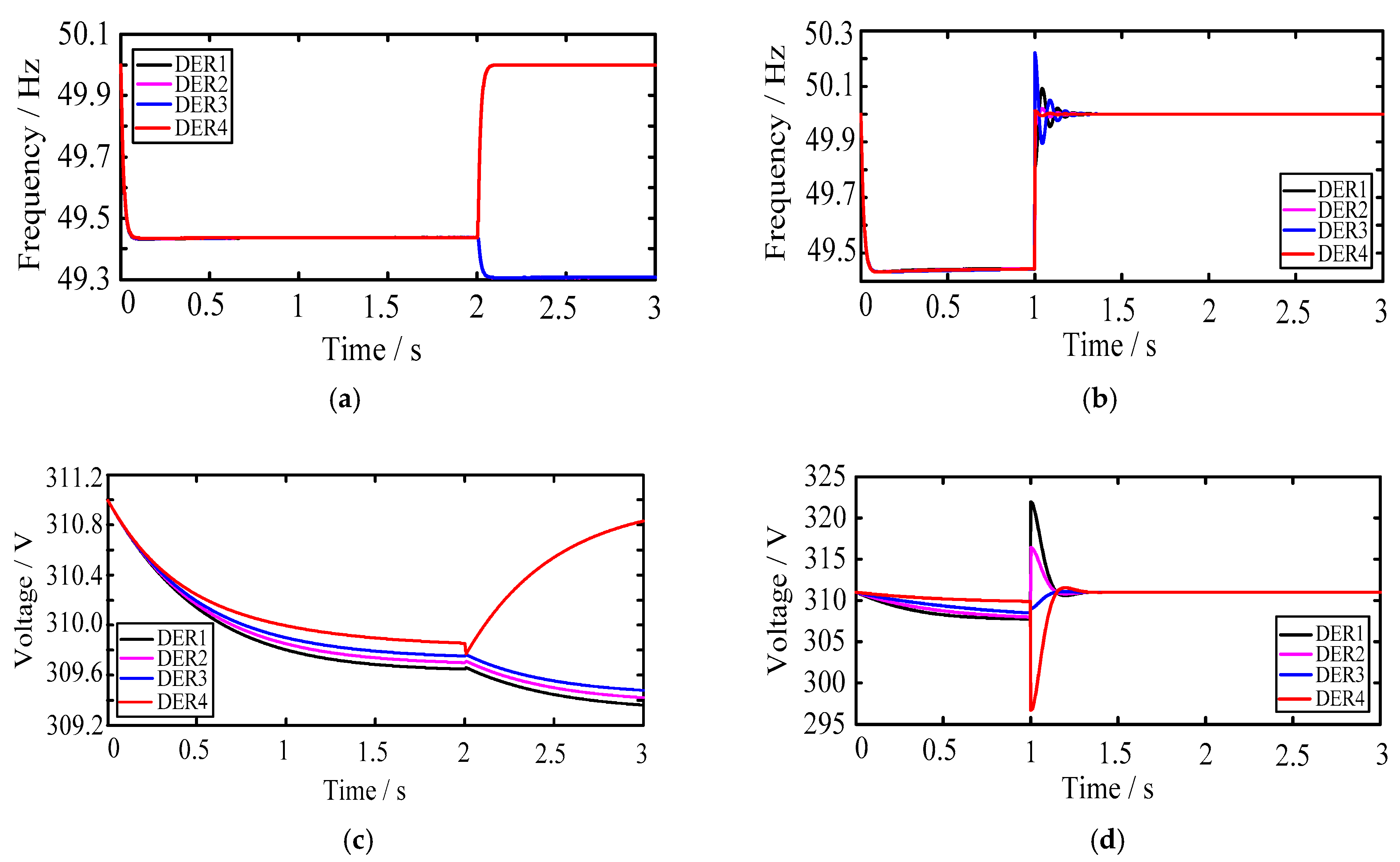
Figure 10.
Variations of output power of DERs when Load disturbance occurs in the system. (a) The output active power of DERs with increasing Load2; (b) The output reactive power of DERs with increasing Load2; (c)The output active power of DERs with decreasing Load2; (d) The output reactive power of DERs with decreasing Load2.
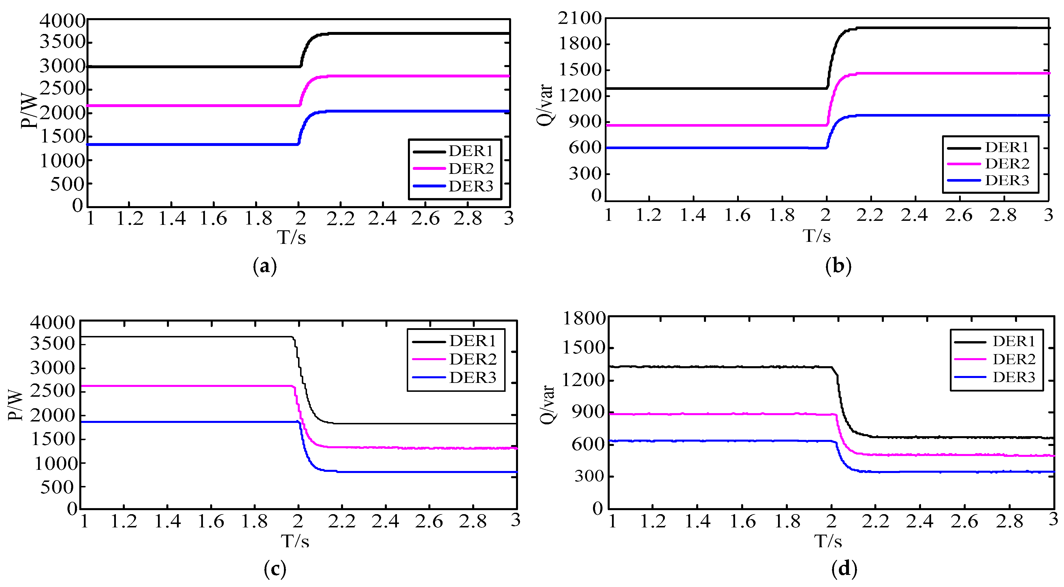
Figure 11.
Variations of output power of DERs when DER disturbance occurs in the system. (a) The output active power of DERs with increasing Load2; (b) The output reactive power of DERs with increasing Load2; (c) The output active power of DERs with decreasing Load2; (d) The output reactive power of DERs with decreasing Load2.
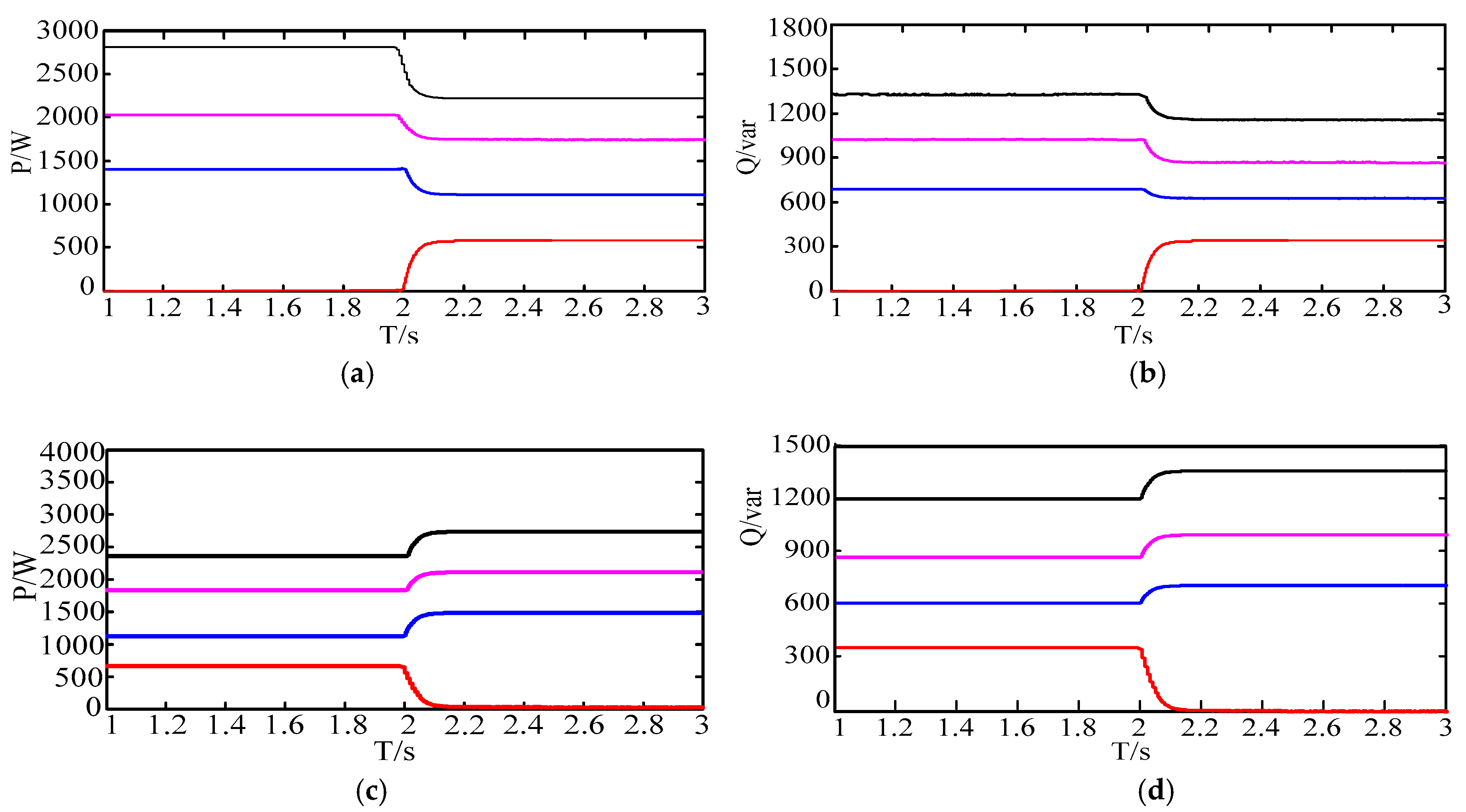
Figure 12.
Control effect on designed sliding mode control (SMC) and coordinated controller. (a) The variations of node voltages of DERs without using SMC when increasing Load2 at t = 2 s; (b) The variations of node voltages of DERs when increasing Load2 at t = 2 s; (c) The variations of node voltages of DERs when cutting off Load2 at t = 2 s; (d) The circumfluence of the node.


Table 1.
Experiment parameters.
| Parameter | Description | Parameter | Description |
|---|---|---|---|
| Power | Line impedance | ||
| Wave filter | |||
| Load1 (always on) | Reference value | ||
| Load2 | Droop coefficient | ||
| Gains in consistency protocol |
© 2018 by the authors. Licensee MDPI, Basel, Switzerland. This article is an open access article distributed under the terms and conditions of the Creative Commons Attribution (CC BY) license (http://creativecommons.org/licenses/by/4.0/).
Share and Cite
MDPI and ACS Style
Yang, Q.; Yuan, D.; Guo, X.; Zhang, B.; Zhi, C. A Novel Hierarchical Control Strategy for Low-Voltage Islanded Microgrids Based on the Concept of Cyber Physical System. Energies 2018, 11, 1835. https://doi.org/10.3390/en11071835
AMA Style
Yang Q, Yuan D, Guo X, Zhang B, Zhi C. A Novel Hierarchical Control Strategy for Low-Voltage Islanded Microgrids Based on the Concept of Cyber Physical System. Energies. 2018; 11(7):1835. https://doi.org/10.3390/en11071835
Chicago/Turabian StyleYang, Qiuxia, Dongmei Yuan, Xiaoqiang Guo, Bo Zhang, and Cheng Zhi. 2018. "A Novel Hierarchical Control Strategy for Low-Voltage Islanded Microgrids Based on the Concept of Cyber Physical System" Energies 11, no. 7: 1835. https://doi.org/10.3390/en11071835
Note that from the first issue of 2016, this journal uses article numbers instead of page numbers. See further details here.