Scalable Clustering of Individual Electrical Curves for Profiling and Bottom-Up Forecasting


1
LMO, University Paris-Sud, 91405 Orsay, France
2
ERIC EA 3083, University de Lyon, Lyon 2, 69676 Bron, France
3
EDF R & D, LMO, Univ Paris-Sud, 91405 Orsay, France
4
University Paris Descartes & LMO, Univ. Paris-Sud, 91405 Orsay, France
*
Author to whom correspondence should be addressed.
Energies 2018, 11(7), 1893; https://doi.org/10.3390/en11071893
Submission received: 29 June 2018
/
Revised: 12 July 2018
/
Accepted: 16 July 2018
/
Published: 20 July 2018
(This article belongs to the Special Issue Short-Term Load Forecasting by Artificial Intelligent Technologies)
Abstract
:Smart grids require flexible data driven forecasting methods. We propose clustering tools for bottom-up short-term load forecasting. We focus on individual consumption data analysis which plays a major role for energy management and electricity load forecasting. The first section is dedicated to the industrial context and a review of individual electrical data analysis. Then, we focus on hierarchical time-series for bottom-up forecasting. The idea is to decompose the global signal and obtain disaggregated forecasts in such a way that their sum enhances the prediction. This is done in three steps: identify a rather large number of super-consumers by clustering their energy profiles, generate a hierarchy of nested partitions and choose the one that minimize a prediction criterion. Using a nonparametric model to handle forecasting, and wavelets to define various notions of similarity between load curves, this disaggregation strategy gives a 16% improvement in forecasting accuracy when applied to French individual consumers. Then, this strategy is implemented using R—the free software environment for statistical computing—so that it can scale when dealing with massive datasets. The proposed solution is to make the algorithm scalable combine data storage, parallel computing and double clustering step to define the super-consumers. The resulting software is openly available.
1. Introduction
1.1. Industrial Context
Energy systems are facing a revolution and many challenges. On the one hand, electricity production is moving to more intermittency and complexity with the increase of renewable energy and the development of small distributed production units such as photovoltaic panels or wind farms. On the other hand, consumption is also changing with plug-in (hybrid) electric vehicles, heat pumps, the development of new technologies such as smart phones, computers, robots that often come with batteries. To maintain the electricity quality, energy stakeholders are developing smart grids (see [1,2]), the next generation power grid including advance communication networks and associated optimisation and forecasting tools. A key component of the smart grids are smart meters. They allow two-sided communication with the customers, real time measurement of consumption and a large scope of demand side management services. A lot of countries have deployed smart meters, as stated in [3], the UK, the US and China have respectively deployed 2.9, 70 and 96 million of such equipments in 2016. In France, 35 million will be deployed before 2021 for a global cost of 5 billion (see e.g., [4]). Ref. [5] mentions that Sweden and Italy have achieved full deployment and [6] that Italian distribution system operators are planning the second wave of roll-outs.
This results in new opportunities such as local optimisation of the grid, demand side management and smart control of storage devices. Exploiting the smart grid efficiently requires advanced data analytics and optimisation techniques to improve forecasting, unit commitment, and load planning at different geographical scales. Massive data sets are and will be produced as explained in [7]: data from energy consumption measured by smart meters at a high frequency (every half minute instead of every 6 months); data from the grid management (e.g., Phasor Measurement Units); data from energy markets (prices and bidding, transmission and distribution system operators data, such as balancing and capacity); data from production units and equipments for their maintenance and control (sensors, periodic measures...). A lot of efforts are made by utilities to develop datalakes and IT structures to gather and make these data available for their business units in real time. Designing new algorithms to analyse and process these data at scale is a key activity and a real competitive advantage.
We will focus on individual consumption data analysis which plays a major role for energy management and electricity load forecasting, designing marketing offers and commercial strategies, proposing new services as energy diagnostics and recommendations, detect and prevent non-technical losses.
1.2. Individual Electrical Consumption Data: A State-of-the-Art
Individual consumption data analysis is, according to the development of smart meters, a popular and growing field of research. Composing an exhaustive survey of recent realizations is then a difficult challenge not addressed here. As detailed in [3], individual consumption data analytics covers various fields of statistics and machine learning: time series, clustering, outlier detection, deep learning, matrix completion, online learning among others.
Given a data set of individual consumptions, a first natural step is exploratory: clustering, which is the most popular unsupervised learning approach. The purpose of clustering is to partition a dataset into homogeneous subsets called clusters (see [8]). Homogeneity is measured according to various criteria such as intra and inter class variances, or distance/dissimilarity measures. The elements of a given cluster are then more similar to those of the same cluster than the elements of the other clusters. Time series clustering is an active subfield where each individual is not characterised by a set of scalar variables but are described by time series, signals or functions, considered as a whole, opening the way for signal processing techniques or functional data analysis methods (see [9,10] for general surveys).
Clustering methods for electricity load data have been widely applied for profiling or demand response management. Refs. [11,12] give an overview of the clustering techniques for customer grouping, finding patterns into electricity load data or detecting outliers and apply it to 400 non-residential medium voltage customers. Clustering can be seen as longitudinal when the objective is to cluster temporal patterns (e.g., daily load curves) from a single individual or transversal when the goal is to build clusters of customers according to their load consumption profile and/or side information. The main application of clustering is load profiling which is essential for energy management, grid management and demand response (see [13]). For example, in [14] data mining techniques are applied to extract load profiles from individual load data of a set of low voltage Portuguese customers, and then supervised classification methods are used to allocate customers to the different classes. In [15], load profiles are obtained by iterative self-organizing data analysis on metered data and demonstrated on a set of 660 hourly metered customers in Finland. Ref. [16] proposes an unsupervised clustering approach based on k-means on features obtained by average seasonal curves using minute metered data from 103 homes in Austin, TX. Correspondence between clusters, their associated profiles and survey data are also studied. Authors of [17] suggest a k-means clustering to derive daily profiles from 220,000 homes and a total of 66 millions daily curves in California. Other approaches based on mixture models are presented in [18] for customers categorization and load profiling on a data set of 2613 smart metered household from London.
Another interest of clustering is forecasting, more precisely bottom-up forecasting which means forecasting the total consumption of a set of customers using individual metered data. Forecasting is an obvious need for optimisation of the grid. As pointed previously, it becomes more and more challenging but also crucial to forecast electricity consumption at different “spatial” scale (a district, a city, a region but also a segment of customers). Bottom up methods are a natural approach consisting of building clusters, forecasting models in each cluster and then aggregating them. In [19], clustering algorithms are compared according to their forecasting accuracy on a data set consisting of 6000 residential customers and SME in Ireland. Good performances are reached but the proposed clustering methods are defined quite independently of the model used for forecasting. On the same data set, Ref. [20] associate a longitudinal clustering and a functional forecasting model similar to KWF (see [21]) for forecasting individual load curves.
A clustering method supervised by forecasting accuracy is proposed in [22] to improve the forecast of the total consumption of a French industrial subset obtaining a substantial gain but suffering from high computational time. In [23], a k-means procedure is applied on features consisting of mean consumption for 5 well chosen periods of day, mean consumption per day of a week and peak position into the year. In each cluster a deep learning algorithm is used for forecasting and then the bottom up forecast is the simple sum of clusters forecasts. Results showing a minimum gain of 11% in forecast accuracy are provided on the Irish data set and smart meter data from New-York. On the Irish data again, Ref. [3] propose to build an ensemble of forecasts from a hierarchical clustering on individual average weekly profiles, coupled with a deep learning model for forecasting in each cluster. Different forecasts corresponding to different sizes of the partition are at the end aggregated using linear regression.
We propose here a new approach, following the previous work of [24], to build clusters and forecasting models that are performant for the bottom-up forecasting problem as well as from the computational point of view.
The paper is organized as follows. After this first section introducing the industrial context and a state-of-the-art review of individual electrical data analysis, Section 2 provides the big picture of our proposal for bottom-up forecasting from smart meter data, without technical details. The next three sections focus on the main tools: wavelets (Section 3) to represent functions and to define similarities between curves, the nonparametric forecasting method KWF (Section 4) and the wavelet-based clustering tools to deal with electrical load curves (Section 5). Section 6 is specifically devoted to the upscaling issue and strategy. Section 7 describes an application for forecasting a French electricity dataset. Finally, Section 8 collects some elements of discussion. It should be noted that we tried to write the paper in such a way that each section could be read independently of each other. Conversely, some sections could be skipped by some readers, without altering the local consistency of the others.
2. Bottom-Up Forecasting from Smart Meter Data: Big Picture
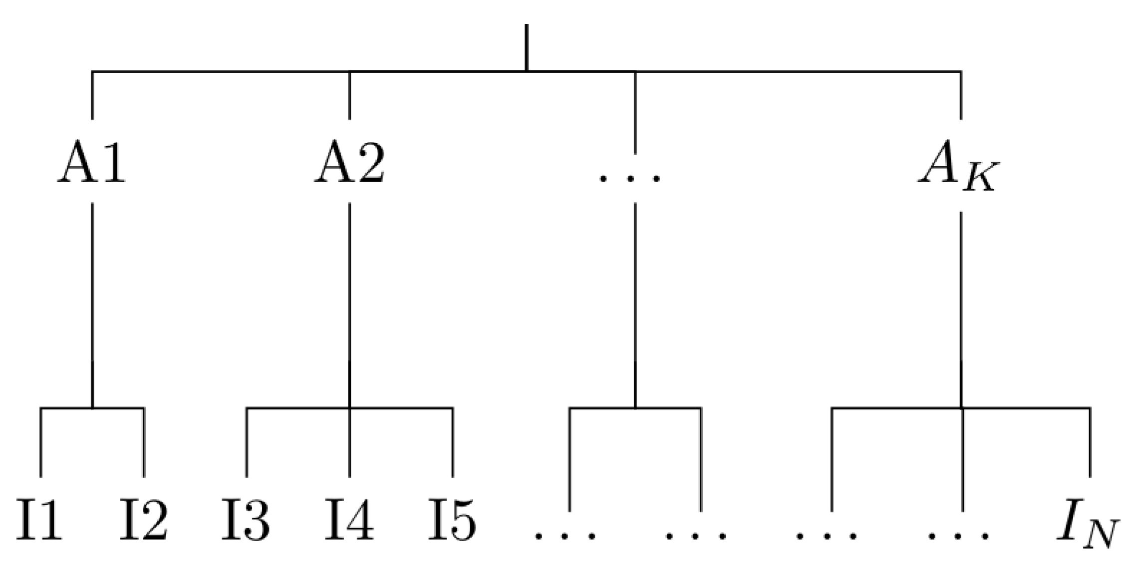
We present here our procedure to get a hierarchical partition of individual customers, schematically represented in Figure 1. On the bottom line, there are N individual customers, say . Each of them has an individual demand coded into an electrical load curve. At the top of the schema, there is one single global demand G obtained by the simple aggregation of the individual ones at each time step, i.e., . We look for the construction of a set of K medium level aggregates, such that they form a partition of the individuals. Each of the considered entities (individuals, medium level aggregates and global demand) can be considered as time series since they carry important time dependent information.
Seasonal univariate time series can naturally be partitioned with regards to time. For example, electrical consumption could be viewed as a sequence of consecutive daily curves which exhibit rich information related to calendar, weather conditions or tariff options. Functional data analysis and forecasting is then a very elegant method to consider. Ref. [25] propose a non-parametric functional method called KWF (Kernel + Wavelet + Functional) to cope with nonstationary time series. Briefly, the main idea is to see the forecasts as a weighted mean of futures of past situations. The weights are obtained according to a similarity index between past curves and actual ones.
Pattern research-based methods repose on a fully non parametric and thus more general frame than prediction approaches more adapted to electricity load demand. This point can be seen as both a weakness and a strength. Specific models can better express the known dependences of electricity demand to long-term trend, seasonal components (due to the interaction of economic and social activities) and climate. However, they usually need more human time to be calibrated. The arrival of new measurement technologies structure of intelligent networks, with more local and high resolution information, unveils forecasting electricity consumption at local scale.
Several arguments can be given to prefer bottom-up approaches with respect to some descending alternatives. Let us briefly mention two of them. The first is related to electrical individual signals themselves which need to be smoothed and the most natural and interpretable way is to define small aggregates of individuals leading to more stable signals, easier to analyse and to forecast (see [17]). The second reason is more statistically related and refers to descending clustering strategies which involve supervised strategies which appear to be especially time consuming (see [22]).
Bottom-up forecasting methods are composed of two successive steps: clustering and forecasting. In the clustering step, the objective is to infer classes from a population such that each class could be accurately forecast. Typically, each class corresponds to customers with specific daily/weekly profile, different relationships to temperature, tariff options or prices (see e.g., [26] regarding demand response). The second step consists in aggregating forecasts to predict the total or any subtotal. In the context of demand response and distribution grid management it could be forecasting the consumption of a district, a town or a substation on the distribution grid.
Recently, Ref. [24] suggested a clustering method achieving both clustering and forecasting of a population of individual customers. They decompose the total consumption such that the sum of disaggregated forecasts improves significantly the forecast of the total. The strategy includes three steps: in the first one super-consumers are designed with a greedy but computationally efficient clustering, then a hierarchical partitioning is done and among which the best partition is chosen according to a disaggregated forecast criterion. The predictions are made with the KWF model which allows one to use it as a off-the-shelve tool.
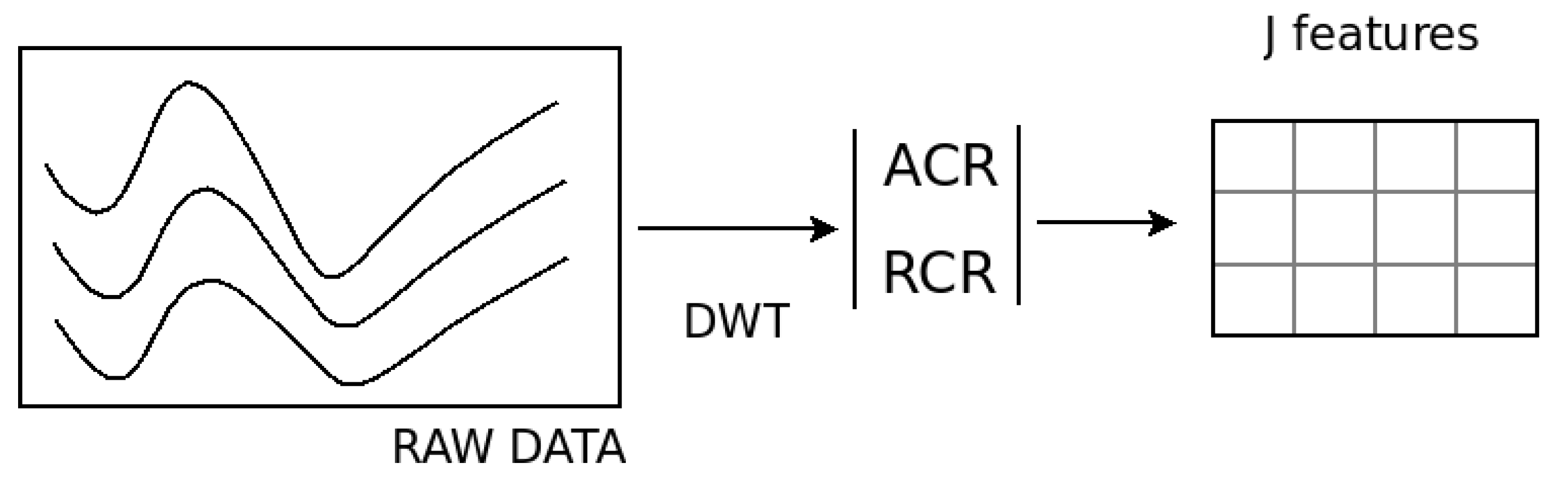
In concrete, data for each customer is a set of P time dependent (potentially noisy) records evenly sampled at a relatively high frequency (e.g., 1/4, 1/2 or hourly records). Then, we consider the data for each individual as a time series that we treat as a function of time. Wavelets are used to code the information about the shape of the curves. Thanks to nice mathematical properties of wavelets, we compress the information of each curve into a handy number of coefficients (in total ) that are called relative energetic contributions. The compression is such that discriminative power is kept even if information is lost. Data are so tabulated in a matrix where lines correspond to observations and columns to variables (see Figure 2).
3. Wavelets
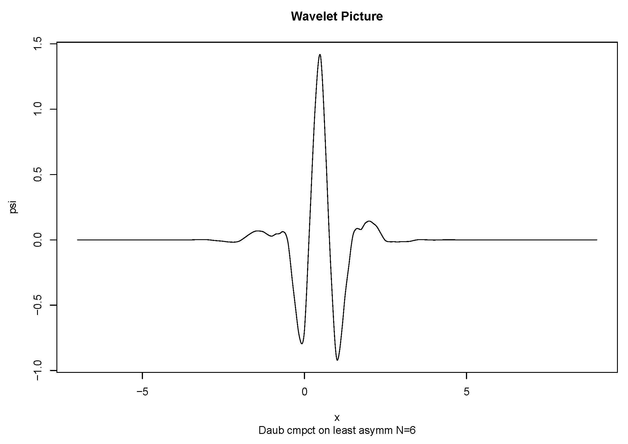
A wavelet is a sufficiently regular and well localized function verifying a simple admissibility condition. During a certain time a wavelet oscillates like a wave and is then localized in time due to a damping. Figure 3 represents the Daubechies least-asymmetric wavelet of order 6. From this single function , using translation and dilation a family of functions that form the basic atoms of the Continuous Wavelet Transform (CWT) is derived From this single function , a family of functions is derived using translation and dilation that form the basic atoms of the Continuous Wavelet Transform (CWT)
For a function of finite energy we define its CWT by the function of two real-valued variables:
Each single coefficient measures the fluctuations of function f at scale a, around the position b. Figure 4 gives a visual representation of , also known as wavelet spectrum, for a 10 day period of load demand sampled at 30 min. The waves that one can visually find on the image indicate the highest zone of fluctuations which corresponds to the days. CWT is then extremely redundant but it is useful for example, to characterize the Holderian regularity of functions or to detect transient phenomena or change-points. A more compact wavelet transform can also be defined.
The Discrete Wavelet Transform is a technique of hierarchical decomposition of the finite energy signals. It allows representing a signal in the time-scale domain, where the scale plays a role analogous to that of the frequency in the Fourier analysis ([27]). It allows to describe a real-valued function through two objects: an approximation of this function and a set of details. The approximation part summarizes the global trend of the function, while the localized changes (in time and frequency) are captured in the detail components at different resolutions. The analysis of signals is carried out by wavelets obtained as before from simple transformations of a single well-localized (both in time and frequency) mother wavelet. A compactly supported wavelet transform provides with an orthonormal basis of waveforms derived from scaling (i.e., dilating or compressing) and translating a compactly supported scaling function and a compactly supported mother wavelet . If one works over the interval , periodized wavelets are useful denoting by
the periodized scaling function and wavelet, that we dilate or stretch and translate
For any , the collection
is an orthonormal basis of . Then, for any function , the orthogonal basis allows one to write the development
where and are called respectively the scale and the wavelet coefficients of z at the position k of the scale j defined as
The wavelet transform can be efficiently computed using the notion of mutiresolution analysis of (MRA), introduced by Mallat, who also designed a family of fast algorithms (see [27]). Using MRA, the first term at the right hand side of (1) describe a smooth approximation of the function z at a resolution level while the second term is the approximation error. It is expressed as the aggregation of the details at scales . If one wants to focus on the finer details then only the information at the scales is to be looked.
Figure 5 is the multiresolution analysis of a daily load curve. The original curve is represented on the top leftmost panel. The bottom rightmost panel contains the approximation part at the coarsest scale , that is, a constant level function. The set of details are plotted by scale which can be connected to frequencies. With this, the detail functions clearly show the different patterns ranging between low and high frequencies. The structure of the signal is centred on the highest scales (lowest frequencies), while the lowest scale (highest frequencies) keep the noise of the signal.
From a practical point of view, let us suppose for simplicity that each function is observed on a fine time sampling grid of size (if not, one may interpolate data to the next power of two). In this context we use a highly efficient pyramidal algorithm ([28]) to obtain the coefficients of the Discrete Wavelet Transform (dwt). Denote by the finite dimensional sample of the function z. For the particular level of granularity given by the size N of the sampling grid, one rewrites (1) using the truncation imposed by the points and the coarser approximation level , as:
Hence, for a given wavelet and a coarse resolution , one may define the dwt operator:
with . Since the dwt operator is based on an -orthonormal basis decomposition, the energy of a square integrable signal is preserved:
Hence, the global energy of is distributed over some energetic components. The key fact that we are going to exploit is how these energies are distributed and how they contribute to the global energy of a signal. Then we can generate a handy number of features that are going to be used for clustering.
4. KWF
4.1. From Discrete to Functional Time Series
Theoretical developments and practical applications associated with functional data analysis were mainly guided by the case of independent observations. However, there is a wide range of applications in which this hypothesis is not reasonable. In particular, when we consider records on a finer grid of time assuming that the measures come from a sampling of an underlying unknown continuous-time signal.
Formally, the problem can be written by considering a continuous stochastic process . So the information contained in a trajectory of X observed on the interval , is also represented by a discrete-time process where comes from the segmentation of the trajectory X in n blocks of size ([29]). Then, the process Z is a time series of functions. For example, we can forecast from the data . This is equivalent to predicting the future behaviour of the X process over the entire interval by having observed X on . Please note that by construction, the are usually dependent functional random variables.
This framework is of particular interest in the study of electricity consumption. Indeed, the discrete consumption measurements can naturally be considered as a sampling of the load curve of an electrical system. The usual segment size, day, takes into account the daily cycle of consumption.
In [21], the authors proposed a prediction model for functional time series in the presence of non stationary patterns. This model has been applied to the electricity demand of Electricité de France (EDF). The general principle of the forecasting model is to find in the past, situations similar to the present and linearly combine their futures to build the forecast. The concept of similarity is based on wavelets and several strategies are implemented to take into account the various non stationary sources. Ref. [30] proposes for the same problem to use a predictor of a similar nature but applied to a multivariate process. Next, [31] provide an appropriate framework for stationary functional processes using the wavelet transform. The latter model is adapted and extended to the case of non-stationary functional processes ([32]).
Thus, a forecast quality of the same order of magnitude as other models used by EDF is obtained for the national curve (highly aggregated) even though our model can represent the series in a simple and parsimonious way. This avoids explicitly modeling the link between consumption and weather covariates, which are known to be important in modeling and often considered essential to take into account. Another advantage of the functional model is its ability to provide multi-horizon forecasts simultaneously by relying on a whole portion of the trajectory of the recent past, rather than on certain points as univariate models do.
4.2. Functional Model KWF
4.2.1. Stationary Case
We consider a stochastic process assumed for the moment, to be stationary, with values in a functional space H (for example ). We have a sample of n curves and the goal is to forecast . The forecasting method is divided in two steps. First, find among the blocks of the past those that are most similar to the last observed block. Then build a weight vector and obtain the desired forecast by averaging the future blocks corresponding to the indices respectively.
First step.
To take into account in the dissimilarity the infinite dimension of the objects to be compared, the KWF model represents each segment , by its development on a wavelet basis truncated to a scale . Thus, each observation is described by a truncated version of its development obtained by the discrete wavelet transform (DWT):
The first term of the equation is a smooth approximation to the resolution of the global behaviour of the trajectory. It contains non-stationary components associated with low frequencies or a trend. The second term contains the information of the local structure of the function. For two observed segments and , we use the dissimilarity D defined as follows:
Since the Z process is assumed to be stationary here, the approximation coefficients do not contain useful information for the forecast since they provide local averages. As a result, they are not taken into account in the proposed distance. In other words, the dissimilarity D makes it possible to find similar patterns between curves even if they have different approximations.
Second step.
Denote the set of scaling coefficients of the i-th segment at the finer resolution J. The prediction of scaling coefficients (at the scale J ) of is given by:
where K is a probability kernel. Finally, we can apply the inverse transform of the DWT to to obtain the forecast of the curve in the time domain. If we note
these weights allow to rewrite the predictor as a barycentre of future segments of the past:
4.2.2. Beyond the Stationary Case
In the case where Z is not a stationary functional process, some adaptations in the predictor (6) must be made to account for nonstationarity. In Antoniadis et al, (2012) corrections are proposed and their efficiency is studied for two types of non-stationarities: the presence of an evolution of the mean level of the approximations of the series and the existence of classes segments. Let us now be more precise.
It is convenient to express each curve according to two terms and describing respectively the approximation and the sum of the details,
When the curves have very different average levels, the first problem appears. In this case, it is useful to centre the curves before calculating the (centred) prediction, and then update the forecast in the second phase. Then, the forecast for the segment is . Since the functional process is centred, we can use the basic method to obtain its prediction
where the weights are given by (5). Then, to forecast we use
To solve the second problem, we incorporate the information of the groups in the prediction stage by redefining the weights according to the belonging of the functions m and n to the same group:
where is equal to 1 if the groups of the n-th segment is equal to the group of the m-th segment and zero elsewhere. If the groups are unknown, they can be determined from an unsupervised classification method.
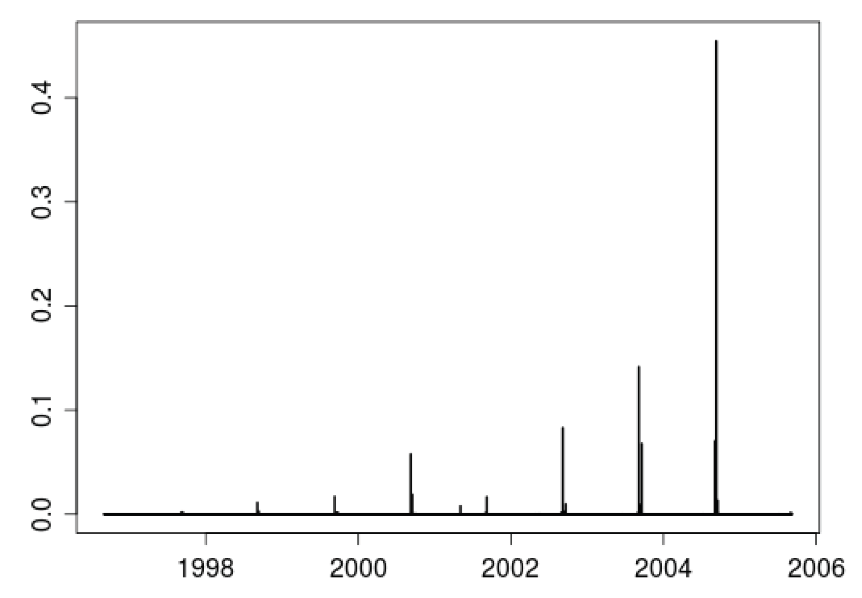
The weight vector can give an interesting insight into the prediction power carried out by the shape of the curves. Figure 6 represents the computed weights obtained for the prediction of a day during Spring 2007. When plotted against time, it is clear that the only days found similar to the current one are located in a remarkably narrow position of each year in the past. Moreover, the weights seem to decrease with time giving more relevance to those days closer to the prediction past. A closer look at the weight vector (not shown here) reveals that only days in Spring are used. Please note that no information about the position of the year was used to compute the weights. Only the information coded in the shape of the curve is necessary to locate the load curve at its effective position inside the year.
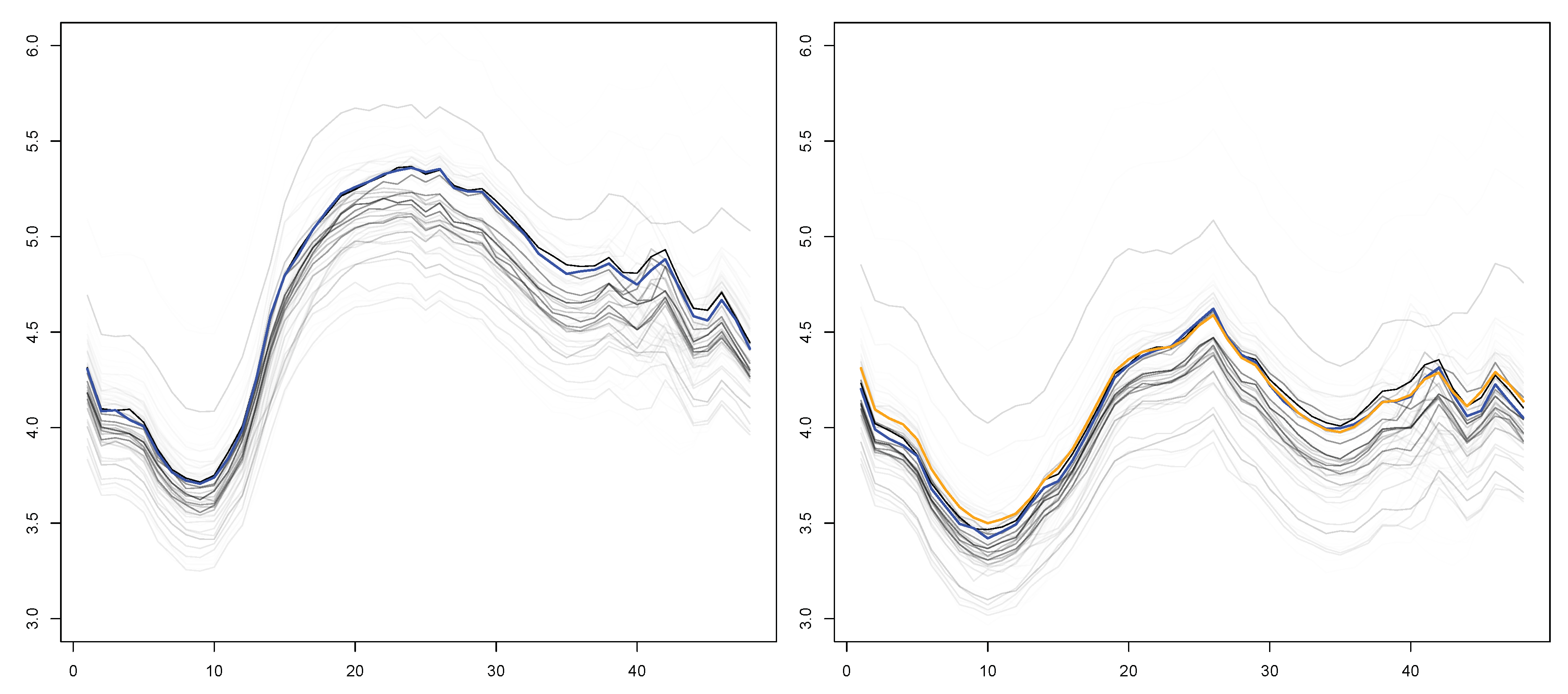
Figure 7 is also of interest to understand how the prediction works. There, the plot on the left contains all the days of the dataset against which the similarity was computed with respect to the curve in blue. A transparency scale which makes visible only those curves with a relatively high similarity index. The plot on the right contains the futures of the past days on the left. These are also plot on the transparent scale with the curve in orange which is the prediction given by the weighted average.
5. Clustering Electrical Load Curves
Individual load prediction is a difficult task as individual signals have a high volatility. The variability of each individual demand is such that the ratio signal to noise decreases dramatically when passing from aggregate to individual data. With almost no hope of predicting individual data, an alternative strategy is to use these data to improve the prediction of the aggregate signal. For this, one may rely on clustering strategies where customers of similar consumption structure will be put into classes in order to form groups of heterogeneous clients. If the clients are similar enough, the signal of the aggregate will gain in regularity and thus in predictability.
Many clustering methods exist in the specialized literature. We adopt the point of view of [33] where two strategies for clustering functional data using wavelets are presented. While the first one allows to rapidly create groups using a dimension reduction approach, the second one permits to better exploit the time-frequency information at the price of some computational burden.
5.1. Clustering by Feature Extraction
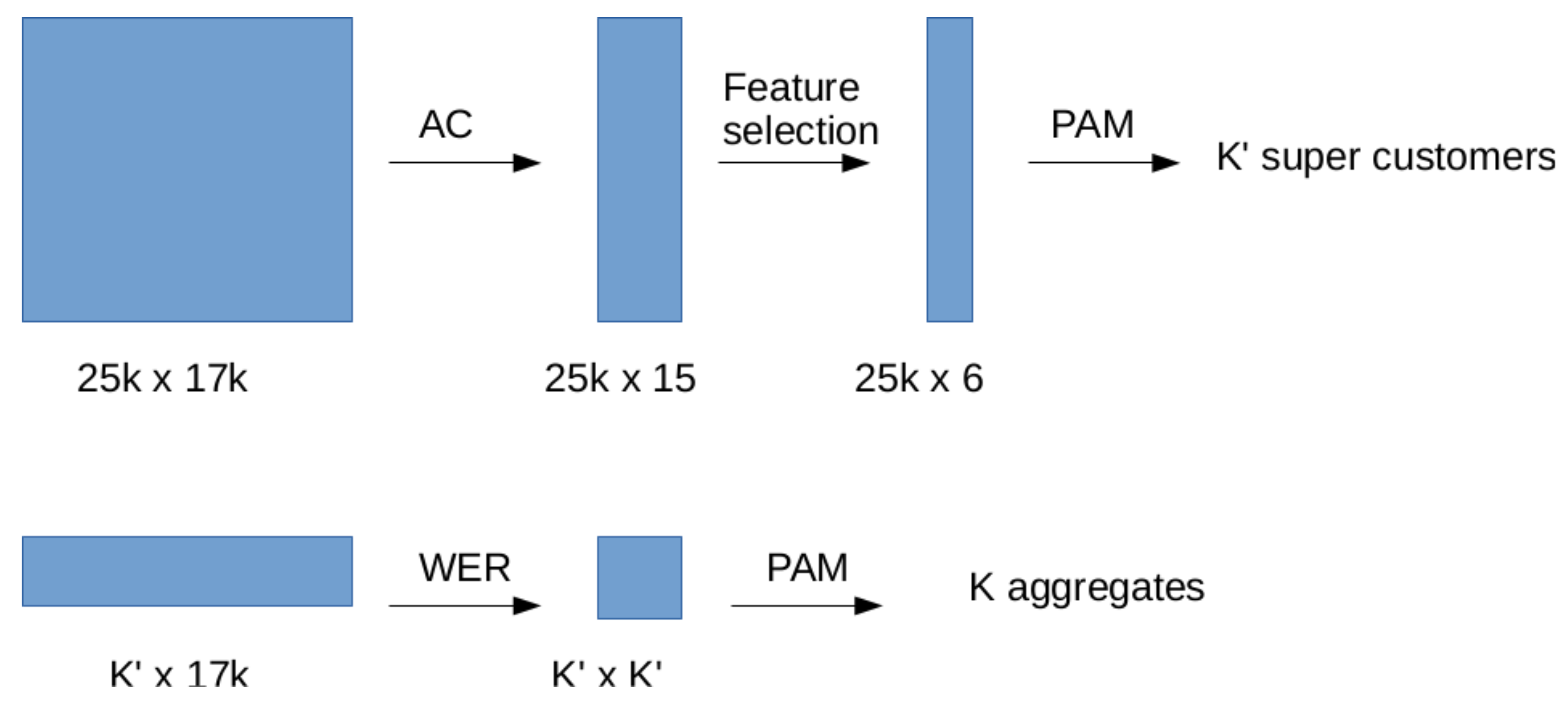
From Equation (3), we can see that the global energy of the curve is approximately decomposed into energy components associated with the smooth approximation of the curve () plus a set of components related to each detail level. In [33] these detail levels were called the absolute contributions of each scale to the global energy of the curve. Notice that the approximation part is not of primary interest since the underlying process of electrical demand may be highly non stationary. With this, we focus only on the shape of the curves and on its frequency content in order to unveil the structure of similar individual consumers to construct clusters. A normalized version of absolute contributions can be considered, which is called relative contributions and is defined as . After this representation step, the result is depicted by the schema in Figure 2, where the original curves are now embedded into a multi dimensional space of dimension J. Moreover if relative contributions are used, the points are in the simplex of .
Let us describe now the clustering step more precisely. For this any clustering algorithm on multivariate data can be used. Since the time complexity of this step is not only dependant on the sample size N but also on the number of variables P, we choose to detect and remove irrelevant features using a variable selection algorithm for unsupervised learning introduced in [34]. Besides the reduction of the computation time, feature selection allows also to gain in interpretability of the clustering since it highly depends on the data.
The aim of this first clustering step is to produce first a coarse clustering with a rather large quantity of aggregated customers, each of them called super-customer (SC). The synchrone demand—that is to say, the sum of all individual demand curves in a specific group—is computed then in all clusters. A parallel can be drawn with the primary situation: we now obtain coarsely aggregated demands over P features, that can be interpreted as a discrete noisy sampling of a curve.
Figure 8 shows this first clustering round on the first row of the schema.
5.2. Clustering Using a Dissimilarity Measure
The second clustering stage consists in grouping the SC into a small quantity K of (super-)aggregates, and building a hierarchy of partitions—as seen before. We consider the samples as functional objects and thus define a dissimilarity between curves, to obtain a dissimilarity matrix between the SC. The projection alternative (working with coefficients) was discarded because of the loss of information.
Following [33] we use the wavelet extended based distance (WER) which is constructed on top of the wavelet coherence. If and are two signals, the wavelet coherence between them is defined as
where is the cross-wavelet transform, and S is a smooth operator. Then, the wavelet coherence can be seen as a linear correlation coefficient computed in the wavelet domain and so localized both in time and scale. Notice that smoothing is a mandatory step in order to avoid a trivial constant for all .
The wavelet coherence is then a two dimensional map that quantifies for each time-scale location the strength of the association between the two signals. To produce a single measure of this map, some kind of aggregation must be done. Following the construction of the extended determination coefficient , Ref. [33] propose to use the wavelet extended which can be computed using
Notice that WER is a similarity measure and it can easily be transformed into a dissimilarity one by
where the computations are done over the grids for the locations b and for the scales a.
The boundary scales (smallest and greatest) are generally taken as a power of two which depend respectively on the minimum detail resolution and the size of the time grid. The other values correspond usually to a linear interpolation over a base 2 logarithmic scale.
While the measure is justified by the power of the wavelet analysis, in practice this distance implies heavy computations involving complex numbers and so requires of a larger memory space. This is one of the two reason that renders its use on the original dataset intractable. The second reason is related to the size of the dissimilarity matrix that results from its applications and that grows with the square of the number of time series. Indeed, such a matrix obtained from the SC is largely tractable for a moderate number of super customers of about some hundreds, but it is not if applied on the whole dataset of some tens of millions of individual customers. The trade off between computation time and precision is resolved by a first clustering step that dramatically reduces the number of time series using the RC features; and a second step that introduces the finer but computationally heavier dissimilarity measure on the SC aggregates.
Since (the number of SC) is sufficiently small, a dissimilarity matrix between the SC can be computed in a reasonable amount of time. This matrix is then used as the input of the classical Hierarchical Agglomerative Clustering (HAC) algorithm, used here with the Ward link. Its output corresponds to the desired hierarchy of (super-)customers.
Otherwise, one may use other clustering algorithms that use a dissimilarity matrix as input (for instance Partitioning Around Mediods, PAM) to get an optimal partitioning for a fixed number of clusters. The second row of the scheme in Figure 8 represents this second step clustering.
6. Upscaling
We discuss in this section the ideas we develop to upscale the problem. Our final target is to work over twenty million time-series. For this, we run many independent clustering tasks in parallel, before merging the results to obtain an approximation of the direct clustering. We give proposed solutions that were tested in order to improve the code performance. Some of our ideas proved to be useful for moderate sample sizes (say tens of thousands) but turned to be counter-productive for larger sizes (tens of millions). Of course all these considerations depend heavily on the specific material and technology. We recall that our interest is on relatively standard scientific workstations. The algorithm we use on the first step of the clustering is described below. We then show the results of the profiling of our whole strategy to highlight where are the bottlenecks when one wishes to up-scale the method. We end this section discussing the solutions we proposed.
6.1. Algorithm Description
The massive dataset clustering algorithm is as follows:
- Data serialization. Time series are given in a verbose by-column format. We re-code all of them in a binary file (if suitable), or a database.
- Dimensionality reduction. Each series of length N is replaced by the energetic coefficients defined using a wavelet basis. Eventually a feature selection step can be performed to further reduction on the number of features.
- Chunking. Data is chunked into groups of size at most , where is a user parameter (we use in the next section experiments).
- Clustering. Within each group, the PAM clustering algorithm is run to obtain clusters.
- Gathering. A final run of PAM is performed to obtain mediods, out of the mediods obtained on the chunks..
From these medoids the synchrone curves are computed (i.e., the sum of all curves within each group for each time step), and given on output for the prediction step.
6.2. Code Profiling
Figure 9 gives some timings obtained by profiling the runs of our initial (C) code. To give a clearer insight, we also report the size of the objects we deal with. The starting point is the ensemble of individual records of electricity demand for a whole year. Here, we treat over 25,000 clients sampled half-hourly during a year. The tabulation of these data to obtain a matrix representation suitable to fit in memory take about 7 min. and requires over 30 Gb of memory.
6.3. Proposed Solutions
Two main solutions are to be discussed, concerning the internal data storage strategy and the use of a simple parallelization scheme. The former looks for reducing the communication time of internal operations using serialization. The latter attacks the major bottleneck of our clustering approach, that is the construction of the WER dissimilarity matrix.
The initial format (verbose, by-column) is clearly inappropriate for efficient data processing. There are several options starting from this data format, they imply having all series stored as
- an ASCII file, one sample per line; very fast, but data retrieval will depend on line number;
- a binary format (3 or 4 octets per value); compression is unadvised since it would increase both preprocessing time and (by a large amount) reading times;
- a database (this is the slowest option), so that retrieval can be very quick.
Since we plan to deal with millions of series of thousands time steps, binary files seemed like a good compromise because they can easily fit on disk—and often also in memory. Our R package uses this format internally, although it allows to input data in any of these three shapes. If we were speaking of billions of series of a million time steps or more, then distributed databases would be required. In this case one would only has to fill the database and tell the R package how to access time-series.
The current version is mostly written in R using the parallel package for efficiency, [35]. A partial version written fully in C was slightly faster, but not enough compared to the loss of code clarity. The current R version can handle the 25 millions samples on an overnight computation over a standard desktop workstation—assuming the curves can be stored and accessed quickly. Our implementation is called iecclust is available as open source software.
7. Forecasting French Electricity Dataset
7.1. Data Presentation
We work on the data provided by EDF also used in [24] which is composed of big customers equipped with smart meters. Unfortunately, this dataset is confidential and cannot be shared. Nevertheless we suggest to the reader interested in bottom up electricity consumption forecasting problems to refer to the open data sets listed in [3].
The dataset consists in approximately 25000 half-hourly load consumption series over two years (2009–2010). The first year is used for partitioning and the calibration of our forecasting algorithm, then the second year is used as a test set to simulate a real forecasting use-case.
The initial dataset contains over 25,000 individual load curves. To test the up-scaling ability of our implementation, we create three datasets of sizes 250,000; 2,500,000 and 25,000,000. In other words, we progressively increase the sample sizes by a factor of 10, 100 and 1000 respectively. The creation follows a simple scheme where each individual curve is multiplied by the realization of independent variables uniformly distributed on at each time step. Each curve is then replicated using this scheme by several times equal to the up-scaling factor.
7.2. Numerical Experiments
The first task clustering is crucial for reducing the dimension of the dataset. We give some timings in order to illustrate how our approach can deal with tens of thousands of time series. Of course, the total computation time depends on the technical specification of the structure used to perform the computation. In our case, we restrict ourselves to a standard scientific workstation with 8 physical cores and 70 Gigabits of live memory. We use all the available cores to cluster chunks of 5000 observations following the algorithm described in Section 6 for both the first and second clustering task.
A very simple pretreatment is done in order to eliminate load curves with eventual errors. For this, we measure the standard deviation of the contributions of each curve to keep only the 99% central observations eliminating the extremest ones. With this, too flat curves (maybe constant) consumptions or very wiggle ones are considered to be abnormal.
Table 1 gives mean average running times over 5 replicates for each of the different sample sizes. These figures show that our strategy yields on a linear increment on the computation time with respect to the number of time series. The maximum number of series we treat, that is 25 millions of individual curves, needs about 12 h to achieve the first task clustering.
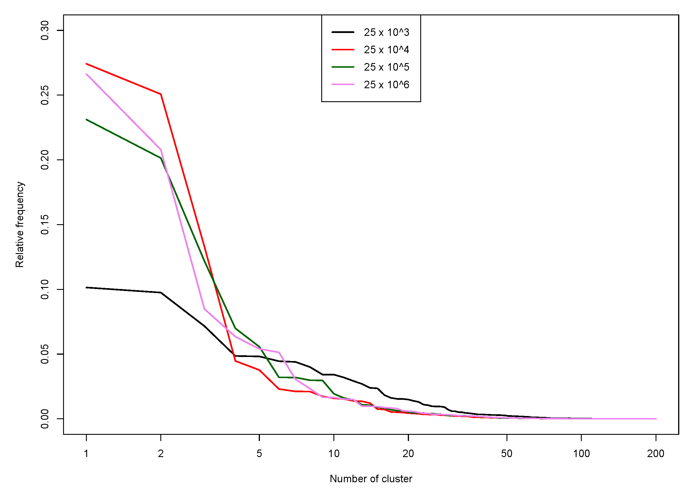
The result of this first clustering task is the load curves of 200 super consumers (SC). We now explore how much time series contains the super consumers. For this, we plot (in Figure 10) the relative frequency of each SC cluster (i.e., proportion of observations in the cluster) against its size rank (in logarithmic scale). With this, the leftmost point of the curve represents the largest cluster, while the following ones are sorted in decreasing order of size. To compare between sample sizes four curves are plotted, one for each sample size. A common decreasing trend of the curves appears producing several relatively small clusters. This is not a desired behaviour for a final clustering task. However, we are in an intermediate step which aims at reducing the number of curves n to a certain number of super customers, here . The isolated super customers may merge together in the following step, producing meaningful aggregates.
In what follows we focus on the results for the largest dataset, which is the one with over 25 millions of load curves. The resulting 200 super consumers are used to construct the WER dissimilarity matrix, which contains rich information about the clustering structure. One may use for instance a hierarchical clustering algorithm to obtain a hierarchy of SC. A graphical result of this structure in the object of Figure 11, which corresponds to the dendrogram obtained by agglomerative hierarchical clustering using the Ward link function. Then, one may get a partitioning of the ensemble of SC by setting some threshold (a value of height in the figure). However, we will not follow this idea to concentrate on the bottom-up prediction task.
The WER dissimilarity matrix encodes rich information about the pairwise closeness between the 200 super consumers. A way to visualize this matrix is to obtain a multidimensional scaling, that is to construct a setting of low dimension coordinates that best represent the dissimilarities between the curves. Figure 12 contains the matrix scatter plot of the first 4 dimensions of such a setting. For each bivariate scatter plot, the points are drawn with a discrete scale of 15 colours, each one representing a different cluster. This low dimensional representation succeed to represent the clustering structure since points with the same colour are closer forming compact groups.
Bottom-up forecast is the leading argument of using the individual load curve clustering. We test the appropriateness of our proposition by getting for a final number of clusters ranging from 2 to 20, 50, 100 and 200 the respective aggregates in terms of load demand. Then, we use KWF as an automatic prediction model for both strategies: prediction of the global demand using the global demand, and the one based on the bottom-up approach.
We use the second year on the dataset to measure the quality of the daily prediction using a rolling basis. Figure 13 reports the prediction error using the MAPE for both the two forecasting strategies. The full horizontal line indicates the annual mean MAPE using the direct method and so it is independent of the number of clusters. For different choices of the number of clusters, the dashed line represent the associated MAPE. All possible clusterings produce then bottom-up forecasts that are better than the one obtained from direct global forecasting.
8. Discussion
In this final section, we discuss the various choices made as well as some possible extension to cope with multiscale model point of view and how to handle non stationarity.
8.1. Choice of Methods
The three main tools are:
- the wavelet decomposition to represent functions and compute dissimilarities. Of course, several other choices could be interesting, such as splines for bases of functions which are independent of the data or even some data-driven bases like those coming from functional principal component analysis. With respect to these two classical alternatives, (more or less related to a monoscale strategy) the choice of wavelets allows simultaneously a parsimonious representation capturing local features of the data as well as redundant one delivering a more accurate multiscale representation. In addition, from a computational viewpoint, DWT is a very fast: of linear complexity. So to design the super-customers the discrete transform is good enough, for the final clusters, the continuous transform leads to better results. Let us remark that combining wavelets and clustering has recently been considered in [36] from a different viewpoint: details and approximations of the daily load curves are clustered separately leading to two different partitions which are then fused.
- the PAM algorithm and the hierarchical clustering to build the clusters are of very common use and well adapted to their specific role in the whole strategy. It should be noted that the use of PAM to construct the super customers must necessarily be biased towards a large number of clusters (defining the super customers) so it is useless to include sophisticated model-selection rules to choose an optimal number of clusters since the strategy is used only to define a sufficiently large number of clusters.
- the Kernel-Wavelet-Functional (KWF) method to forecast time-series. The global forecasting scheme is clearly fully modular and then, KWF could be replaced by any other time-series model forecasting. The model must be flexible and easy to automatically be tuned because the modeling and forecasting must be performed in each cluster in a rather blind way. The main difficulty with KWF is to introduce exogenous variables. We could imagine to include a single one quite easily but not a richer family in full generality. Nevertheless, it is precisely when dealing with models corresponding to some specific clusters that it could be of interest to use exogenous variables especially informative, for example describing meteo at a local level or some specific market segment. Therefore, some alternatives could be considered, such as generalized additive models (see [37] for a strategy which could be plugged into our scheme).
8.2. Multiscale Modeling and Forecasting
In fact, such a forecasting strategy combining clustering in individuals and forecasting of the total consumption of each cluster can be also viewed as a multiscale modeling. Indeed a by-product is a forecasting at different levels of aggregation from the super customers to the total population. Therefore, instead of restricting our attention on the forecasting of the global signal for a given partition we could imagine to combine in time the different predictions given by each piece of the different partitions in such a way that all the levels could contribute to the final forecasting. The way to weight the different predictions could be fixed for all the instants (see [38] for a large choice of proposals) or, on the contrary, time-dependent according to a convenient choice of the updating policy (see the sequential learning strategies already used in the electrical context in [39]). An attempt in this direction can be found in [40].
Another related topic is individual forecasting or prediction. It must be mentioned since it is interesting to have some ideas about the kind of statistical models or strategies used in this especially hard context, due to extreme volatility and wild nonstationarity. Ref. [41] examine the short-term (one hour) forecasting of individual consumptions using a sparse autoregressive model which is compared against well-known alternatives (support vector machine, principal component regression, and random forests). In general, exogenous variables are used to forecast electricity consumptions, but some authors focus on the reverse. Ref. [42,43] are interested in determining household characteristics or customers information based on temporal load profiles of household electricity demand. They use sophisticated deep learning algorithm for the first one and more classical tools for the second one. In the context of customers surveys, Ref. [44] use smart meter data analytics for optimal customer selection in demand response programs.
8.3. How to Handle Non Stationarity?
Even if the model KWF is well suited to handle non stationarities in the time-domain, it remains that the clusters of customers are also subjected to some dynamics which could be of interest to model in order to control these changes. A first naive possibility is to periodically recompute the entire process including a new calculation of the super-customers and decide, at some stage if the change is significant to be taken into account. A second possibility could be to directly model the evolution of the clusters. For example, in [45] a time-varying extension of the K-means algorithm is proposed. A multivariate vector autoregressive model is used to model the evolution of clusters’ centroids over time. This could help to model the changes of clusters along time but we have to think about a penalty mechanism allowing to make changes in the cluster only when it is useful.
Author Contributions
B. Auder, J. Cugliari, Y. Goude and J.-M. Poggi equally contributed to this work.
Acknowledgments
This research benefited from the support of the FMJH ’Program Gaspard Monge for optimization and operations research and their interactions with data science’, and from the support from EDF and Thales.
Conflicts of Interest
The authors declare no conflict of interest.
References
- Yan, Y.; Qian, Y.; Sharif, H.; Tipper, D. A Survey on Smart Grid Communication Infrastructures: Motivations, Requirements and Challenges. IEEE Commun. Surv. Tutor. 2013, 15, 5–20. [Google Scholar] [CrossRef] [Green Version]
- Mallet, P.; Granstrom, P.O.; Hallberg, P.; Lorenz, G.; Mandatova, P. Power to the People!: European Perspectives on the Future of Electric Distribution. IEEE Power Energy Mag. 2014, 12, 51–64. [Google Scholar] [CrossRef]
- Wang, Y.; Chen, Q.; Hong, T.; Kang, C. Review of Smart Meter Data Analytics: Applications, Methodologies, and Challenges. IEEE Trans. Smart Grid 2018. [Google Scholar] [CrossRef]
- Jamme, D. Le compteur Linky: Brique essentielle des réseaux intelligents français. In Proceedings of the Office Franco-Allemand Pour La Transition énergétique, Berlin, Germany, 11 May 2017. [Google Scholar]
- Alahakoon, D.; Yu, X. Smart Electricity Meter Data Intelligence for Future Energy Systems: A Survey. IEEE Trans. Ind. Inform. 2016, 12, 425–436. [Google Scholar] [CrossRef]
- Ryberg, T. The Second Wave of Smart Meter Rollouts Begin in Italy and Sweden. 2017. Available online: https://www.metering.com/regional-news/europe-uk/second-wave-smart-meter-rollouts-begins-italy-sweden/ (accessed on 1 June 2018).
- Jiang, H.; Wang, K.; Wang, Y.; Gao, M.; Zhang, Y. Energy big data: A survey. IEEE Access 2016, 4, 3844–3861. [Google Scholar] [CrossRef]
- Kaufman, L.; Rousseeuw, P. Finding Groups in Data: An Introduction to Cluster Analysis; Wiley: Hoboken, NJ, USA, 1990. [Google Scholar]
- Liao, T.W. Clustering of time series data a survey. Pattern Recognit. 2005, 38, 1857–1874. [Google Scholar] [CrossRef]
- Jacques, J.; Preda, C. Functional Data Clustering: A Survey. Adv. Data Anal. Classif. 2014, 8, 231–255. [Google Scholar] [CrossRef]
- Chicco, G. Overview and performance assessment of the clustering methods for electrical load pattern grouping. Energy 2012, 42, 68–80. [Google Scholar] [CrossRef]
- Zhou, K.; Yang, S.; Shen, C. A review of electric load classification in smart grid environment. Renew. Sustain. Energy Rev. 2013, 24, 103–110. [Google Scholar] [CrossRef]
- Wang, Y.; Chen, Q.; Kang, C.; Zhang, M.; Wang, K.; Zhao, Y. Load profiling and its application to demand response: A review. Tsinghua Sci. Technol. 2015, 20, 117–129. [Google Scholar] [CrossRef]
- Figueiredo, V.; Rodrigues, F.; Vale, Z.; Gouveia, J.B. An electric energy consumer characterization framework based on data mining techniques. IEEE Trans. Power Syst. 2005, 20, 596–602. [Google Scholar] [CrossRef]
- Mutanen, A.; Ruska, M.; Repo, S.; Jarventausta, P. Customer Classification and Load Profiling Method for Distribution Systems. IEEE Trans. Power Deliv. 2011, 26, 1755–1763. [Google Scholar] [CrossRef]
- Rhodes, J.D.; Cole, W.J.; Upshaw, C.R.; Edgar, T.F.; Webber, M.E. Clustering analysis of residential electricity demand profiles. Appl. Energy 2014, 135, 461–471. [Google Scholar] [CrossRef]
- Kwac, J.; Flora, J.; Rajagopal, R. Household Energy Consumption Segmentation Using Hourly Data Smart Grid. IEEE Trans. 2014, 5, 420–430. [Google Scholar]
- Sun, M.; Konstantelos, I.; Strbac, G. C-Vine copula mixture model for clustering of residential electrical load pattern data. In Proceedings of the 2017 IEEE Power Energy Society General Meeting, Chicago, IL, USA, 16–20 July 2017. [Google Scholar] [CrossRef]
- Alzate, C.; Sinn, M. Improved electricity load forecasting via kernel spectral clustering of smartmeter. In Proceedings of the International Conference on Data Mining, Dallas, TX, USA, 7–10 December 2013; pp. 943–948. [Google Scholar]
- Chaouch, M. Clustering-Based Improvement of Nonparametric Functional Time Series Forecasting: Application to Intra-Day Household-Level Load Curves. IEEE Trans. Smart Grid 2014, 5, 411–419. [Google Scholar] [CrossRef]
- Antoniadis, A.; Brossat, X.; Cugliari, J.; Poggi, J.M. Prévision d’un processus à valeurs fonctionnelles en présence de non stationnarités. Application à la consommation d’électricité. J. Soc. Française Stat. 2012, 153, 52–78. [Google Scholar]
- Misiti, M.; Misiti, Y.; Oppenheim, G.; Poggi, J.M. Optimized Clusters for Disaggregated Electricity Load Forecasting. Rev. Stat. J. 2010, 8, 105–124. [Google Scholar]
- Quilumba, F.L.; Lee, W.J.; Huang, H.; Wang, D.Y.; Szabados, R.L. Using Smart Meter Data to Improve the Accuracy of Intraday Load Forecasting Considering Customer Behavior Similarities. IEEE Trans. Smart Grid 2015, 6, 911–918. [Google Scholar] [CrossRef]
- Cugliari, J.; Goude, Y.; Poggi, J.M. Disaggregated Electricity Forecasting using Wavelet-Based Clustering of Individual Consumers. In Proceedings of the 2016 IEEE International Energy Conference (ENERGYCON), Leuven, Belgium, 4–8 April 2016. [Google Scholar]
- Antoniadis, A.; Brossat, X.; Cugliari, J.; Poggi, J.M. Une approche fonctionnelle pour la prévision non-paramétrique de la consommation d’électricité. J. Soc. Française Stat. 2014, 155, 202–219. [Google Scholar]
- Labeeuw, W.; Stragier, J.; Deconinck, G. Potential of active demand reduction with residential wet appliances: A case study for Belgium. Smart Grid IEEE Trans. 2015, 6, 315–323. [Google Scholar] [CrossRef]
- Mallat, S. A Wavelet Tour of Signal Processing; Academic Press: Cambridge, MA, USA, 1999. [Google Scholar]
- Mallat, S. A theory for multiresolution signal decomposition: The wavelet representation. IEEE Trans. Pattern Anal. Mach. Intell. 1989, 11, 674–693. [Google Scholar] [CrossRef]
- Bosq, D. Modelization, nonparametric estimation and prediction for continuous time processes. In Nonparametric Functional Estimation and Related Topics; Roussas, G., Ed.; NATO ASI Series, (Series C: Mathematical and Physical Sciences); Springer: Dordrecht, The Netherland, 1991; Volume 335, pp. 509–529. [Google Scholar]
- Poggi, J.M. Prévision non paramétrique de la consommation électrique. Rev. Stat. Appl. 1994, 4, 93–98. [Google Scholar]
- Antoniadis, A.; Paparoditis, E.; Sapatinas, T. A functional wavelet-kernel approach for time series prediction. J. R. Stat. Soc. Ser. B Stat. Meth. 2006, 68, 837. [Google Scholar] [CrossRef]
- Cugliari, J. Prévision Non Paramétrique De Processus à Valeurs Fonctionnelles. Application à la Consommation D’électricité. Ph.D. Thesis, Université Paris Sud, Orsay, France, 2011. [Google Scholar]
- Antoniadis, A.; Brossat, X.; Cugliari, J.; Poggi, J.M. Clustering functional data using wavelets. Int. J. Wave. Multiresolut. Inform. Proc. 2013, 11. [Google Scholar] [CrossRef]
- Steinley, D.; Brusco, A.M. new variable weighting and selection procedure for k-means cluster analysis. Multivar. Behav. Res. 2008, 43, 32. [Google Scholar] [CrossRef] [PubMed]
- R Core Team. R: A Language and Environment for Statistical Computing; R Foundation for Statistical Computing: Vienna, Austria, 2018. [Google Scholar]
- Jiang, Z.; Lin, R.; Yang, F.; Budan, W. A Fused Load Curve Clustering Algorithm based on Wavelet Transform. IEEE Trans. Ind. Inform. 2017. [Google Scholar] [CrossRef]
- Thouvenot, V.; Pichavant, A.; Goude, Y.; Antoniadis, A.; Poggi, J.M. Electricity forecasting using multi-stage estimators of nonlinear additive models. IEEE Trans. Power Syst. 2016, 31, 3665–3673. [Google Scholar] [CrossRef]
- Polikar, R. Ensemble learning. In Ensemble Machine Learning; Springer: Berlin, Germany, 2012; pp. 1–34. [Google Scholar]
- Gaillard, P.; Goude, Y. Forecasting electricity consumption by aggregating experts; how to design a good set of experts. In Modeling and Stochastic Learning for Forecasting in High Dimensions; Springer: Berlin, Germany, 2015; pp. 95–115. [Google Scholar]
- Goehry, B.; Goude, Y.; Massart, P.; Poggi, J.M. Forêts aléatoires pour la prévision à plusieurs échelles de consommations électriques. In Proceedings of the 50 èmes Journées de Statistique, Paris Saclay, France, 28 May–1 June 2018. talk 112. [Google Scholar]
- Li, P.; Zhang, B.; Weng, Y.; Rajagopal, R. A sparse linear model and significance test for individual consumption prediction. IEEE Trans. Power Syst. 2017, 32, 4489–4500. [Google Scholar] [CrossRef]
- Wang, Y.; Chen, Q.; Gan, D.; Yang, J.; Kirschen, D.S.; Kang, C. Deep Learning-Based Socio-demographic Information Identification from Smart Meter Data. IEEE Trans. Smart Grid 2018. [Google Scholar] [CrossRef]
- Anderson, B.; Lin, S.; Newing, A.; Bahaj, A.; James, P. Electricity consumption and household characteristics: Implications for census-taking in a smart metered future. Comput. Environ. Urban Syst. 2017, 63, 58–67. [Google Scholar] [CrossRef]
- Martinez-Pabon, M.; Eveleigh, T.; Tanju, B. Smart meter data analytics for optimal customer selection in demand response programs. Energy Proc. 2017, 107, 49–59. [Google Scholar] [CrossRef]
- Maruotti, A.; Vichi, M. Time-varying clustering of multivariate longitudinal observations. Commun. Stat. Theory Meth. 2016, 45, 430–443. [Google Scholar] [CrossRef] [Green Version]
Figure 1.
Schematic representation of a hierarchy of customers.

Figure 2.
From curves to matrices.

Figure 3.
Daubechies least-asymmetric wavelet with filter size 6.

Figure 4.
Wavelet spectrum of a week of electrical load demand.

Figure 5.
Multiresolution analysis

Figure 6.
Vector of weights (sorted chronologically) obtained for the prediction of a day during Spring.
Figure 6.
Vector of weights (sorted chronologically) obtained for the prediction of a day during Spring.

Figure 7.
Past and future segments involved in the construction of the prediction by KWF. On each panel, all the days are represented with a transparent colour making visible only the most relevant days for the construction of the predictor.
Figure 7.
Past and future segments involved in the construction of the prediction by KWF. On each panel, all the days are represented with a transparent colour making visible only the most relevant days for the construction of the predictor.

Figure 8.
Two step clustering.

Figure 9.
Code profiling by tasks.
| Task | Time | Memory | Disk |
|---|---|---|---|
| Raw (15 Gb) to matrix | 7 min | 30 Gb | 2.7 Gb |
| Compute contributions | 7 min | <1 Gb | 7 Mb |
| 1st stage clustering | 3 min | <1 Gb | – |
| Aggregation | 1 min | 6 Gb | 30 Mb |
| Wer distance matrix | 40 min | 64 Gb | 150 Kb |
| Forecasts | 10 min | <1 Gb | – |
Figure 10.
Relative frequency of observations by cluster, in decreasing order, for different sample sizes, .
Figure 10.
Relative frequency of observations by cluster, in decreasing order, for different sample sizes, .

Figure 11.
Dendrogram obtained from the WER dissimilarity matrix.

Figure 12.
Multidimensional scaling of the WER dissimilarity matrix for the 200 super consumers.

Figure 13.
MAPE for the aggregate demand by number of classes for the two strategies: direct global demand forecast (full) and bottom-up forecast (dashed).
Figure 13.
MAPE for the aggregate demand by number of classes for the two strategies: direct global demand forecast (full) and bottom-up forecast (dashed).


Table 1.
Mean average running times (over 5 replicates) for different sample sizes (in log).
| Sample Size | Time (In Seconds) |
|---|---|
| 67 | |
| 513 | |
| 4420 | |
| 43,893 |
© 2018 by the authors. Licensee MDPI, Basel, Switzerland. This article is an open access article distributed under the terms and conditions of the Creative Commons Attribution (CC BY) license (http://creativecommons.org/licenses/by/4.0/).
Share and Cite
MDPI and ACS Style
Auder, B.; Cugliari, J.; Goude, Y.; Poggi, J.-M. Scalable Clustering of Individual Electrical Curves for Profiling and Bottom-Up Forecasting. Energies 2018, 11, 1893. https://doi.org/10.3390/en11071893
AMA Style
Auder B, Cugliari J, Goude Y, Poggi J-M. Scalable Clustering of Individual Electrical Curves for Profiling and Bottom-Up Forecasting. Energies. 2018; 11(7):1893. https://doi.org/10.3390/en11071893
Chicago/Turabian StyleAuder, Benjamin, Jairo Cugliari, Yannig Goude, and Jean-Michel Poggi. 2018. "Scalable Clustering of Individual Electrical Curves for Profiling and Bottom-Up Forecasting" Energies 11, no. 7: 1893. https://doi.org/10.3390/en11071893
Note that from the first issue of 2016, this journal uses article numbers instead of page numbers. See further details here.