Uncertainty Analysis of Weather Forecast Data for Cooling Load Forecasting Based on the Monte Carlo Method


Tianjin Key Lab of Indoor Air Environmental Quality Control, School of Environmental Science and Engineering, Tianjin University, Tianjin 300350, China
*
Author to whom correspondence should be addressed.
Energies 2018, 11(7), 1900; https://doi.org/10.3390/en11071900
Submission received: 29 June 2018
/
Revised: 14 July 2018
/
Accepted: 17 July 2018
/
Published: 20 July 2018
(This article belongs to the Special Issue Short-Term Load Forecasting by Artificial Intelligent Technologies)
Abstract
:Recently, the cooling load forecasting for the short-term has received increasing attention in the field of heating, ventilation and air conditioning (HVAC), which is conducive to the HVAC system operation control. The load forecasting based on weather forecast data is an effective approach. The meteorological parameters are used as the key inputs of the prediction model, of which the accuracy has a great influence on the prediction loads. Obviously, there are errors between the weather forecast data and the actual weather data, but most of the existing studies ignored this issue. In order to deal with the uncertainty of weather forecast data scientifically, this paper proposes an effective approach based on the Monte Carlo Method (MCM) to process weather forecast data by using the 24-h-ahead Support Vector Machine (SVM) model for load prediction as an example. The data-preprocessing method based on MCM makes the forecasting results closer to the actual load than those without process, which reduces the Mean Absolute Percentage Error (MAPE) of load prediction from 11.54% to 10.92%. Furthermore, through sensitivity analysis, it was found that among the selected weather parameters, the factor that had the greatest impact on the prediction results was the 1-h-ahead temperature T(h–1) at the prediction moment.
1. Introduction
In recent years, heating, ventilation and air conditioning (HVAC) systems have become important elements in office buildings and are responsible for around 40% of the energy use in office buildings, which means a great energy-saving potential [1]. However, the operation management level of HVAC systems is generally low, and the refrigeration capacity of the equipment does not match with the actual demand, resulting in a large energy consumption. Precise load forecasting is the basis of the optimization of HVAC system operation, which is conducive to formulate an operation strategy according to the load change and can lay the theoretical foundation for enhancing the thermal comfort and reducing the energy consumption of office buildings. Among the influential factors, meteorological parameters play a very important role in the dynamic cooling load, which has a great influence on the actual energy consumption of a building.
In the relevant literature on building load forecasting, various prediction models are proposed for load forecasting and related research. Xia and Xiang et al. [2] proposed a prediction model based on a radial basis function (RBF) neural network to forecast a daily load, which mainly took some weather parameters into consideration including temperature, humidity, wind speed, atmospheric pressure and so on. The forecasting results illustrated that the model has better performance compared with the Back Propagation (BP) network. Ruzic et al. [3] put forward a regression-based adaptive weather-sensitive short-term load-forecasting algorithm. This algorithm was used for the load prediction of the Electric Power Utility of Serbia. Wi [4] presented a fuzzy polynomial regression method for holiday load prediction combined with the dominant weather feature, and pointed out that it was pivotal to select the previous data relevant to the given holiday for improving the accuracy of holiday load forecasting. Support Vector Machines (SVMs) have been widely applied in the field of pattern recognition, bioinformatics, and other artificial intelligence relevant areas to solve the classification and regression issues; these are called Support Vector Classification (SVC) and Support Vector Regression (SVR). Particularly, along with Vapnik’s ε-insensitive loss function, the SVM also has been extended to solve nonlinear regression estimation problems by SVR. It has been widely used in many fields involving prediction problems, such as financial industry forecasting [5,6,7], engineering and software field forecasting [8], atmospheric science forecasting [9] and so on. Furthermore, the SVR model has also been successfully applied to predict the power load [10]. The selection of the three parameters (C, ε, and σ) in the SVR model influences the prediction accuracy significantly. Many studies have given recommendations on appropriate setting of SVR parameters [11]. But those methods do not comprehensively consider the interaction effects among the three parameters. Thus, the intelligent algorithms are adopted to determine appropriate parameter values. Barman et al. [12] proposed a regional hybrid STLF model utilizing SVM with a new technique to evaluate its suitable parameters and pointed out that the GOA-SVM model is targeted for forecasting the load under local climatic conditions. Li et al. [13] investigate the feasibility of using Least Squares Support vector regression (LS-SVR) to forecast building cooling load. The evaluation of the tests illustrated that the SVR model with the Particle Swarm Optimization (PSO) has a good generalization performance.
At present, the research on the inputs of the prediction model mainly involves the optimized selection of input parameters. Duanmu et al. [14] proposed a simplified prediction model of the cooling load based on the hourly cooling load coefficient method and analyzed the various influential factors of the cooling load. They pointed out that outdoor temperature is the key influential factor of the cooling load. Wang et al. [15] researched the influence of climate change on the heating and the cooling (H/C) energy requirements of residential houses, which is from cold to hot humid in five regional climates of Australia. They pointed out that the impacts of significant climate change on H/C energy requirements may occur during the lifecycle of existing housing stock. Jiang [16] considered that the accurate prediction of building thermal performance is dependent on meteorological data such as dry-bulb temperature, relative humidity, wind speed and solar radiation to a large extent. Chen et al. [17] selected different meteorological variables as inputs for different time scales, using building dynamics simulation to forecast the energy demand for cooling and heating of residential buildings. Petersen et al. [18] analyzed the impact of uncertainty on the indoor environment.
Indeed, only a few studies have formally dealt with the issue of uncertainty in load forecasting. For example, Sarjiya [19] adopted a decision analysis method to handle the uncertainty of the load forecast in power systems for the aim of optimization of the operating strategy. Domínguez-Muñoz [20] proposed a new approach based on stochastic simulation methods to research the impact of the uncertainty of the internal disturbance on the peak cooling load in the buildings. Douglas et al. [21] put forward a method to analyze the risk of short-term power system operational planning with the electrical load forecast uncertainty. MacDonald [22] focused on the problem of quantifying the effect of uncertainty on the predictions made by simulation tools. Two approaches including external and internal methods were used to quantify this effect. Domínguez-Muñoz et al. [23] quantified the uncertainty that can be expected in the thermal conductivity of insulation materials in the lack of specific experimental measurements. Sten et al. [24] analyzed the influence of the uncertainties of temperature stratification and pressure coefficients on buildings in term of natural ventilation through an expert review process.
Overviewing the previous research, few studies have paid attention to the influence of uncertainty of weather forecast data on the load forecasting. However, external disturbance factors such as meteorological parameters play a very important role in the dynamic cooling loads of a building, which have a great impact on the actual energy consumption of the building. It is effective to use the weather forecast data to predict the building load in advance and adjust the air conditioning units in time according to the forecast loads for the purposes of improvement of the indoor comfort and reduction of building energy consumption. If the uncertainty of weather forecast data is ignored, it may cause errors in model inputs, which reduces the accuracy of the forecast load. The paper fills a gap in terms of the correction of the uncertainty of weather forecast data.
This paper explored the impact of weather forecast uncertainty on load forecasting, and the Monte Carlo Method (MCM) was used to modify the input parameters of the model for load forecasting, which can increase the accuracy of the load forecasting before and after the correction. Furthermore, the sensitivity analysis was adopted to explore the factors that have a great impact on load forecasting results.
The contents of the paper are as follows. Section 2 presents a general overview of the principles of the MCM, the SVM and sensitivity analysis. Section 3 presents a case study, in which this case study is used to illustrate how the methodology can be applied to study the impact of uncertainty of the weather forecast data on load prediction, and the main factors contributing to the load prediction are identified through a sensitivity analysis. Section 4 presents a discussion of the results, as well as some proposals for future research. Section 5 summarizes two important conclusions in the research.
2. Methodology
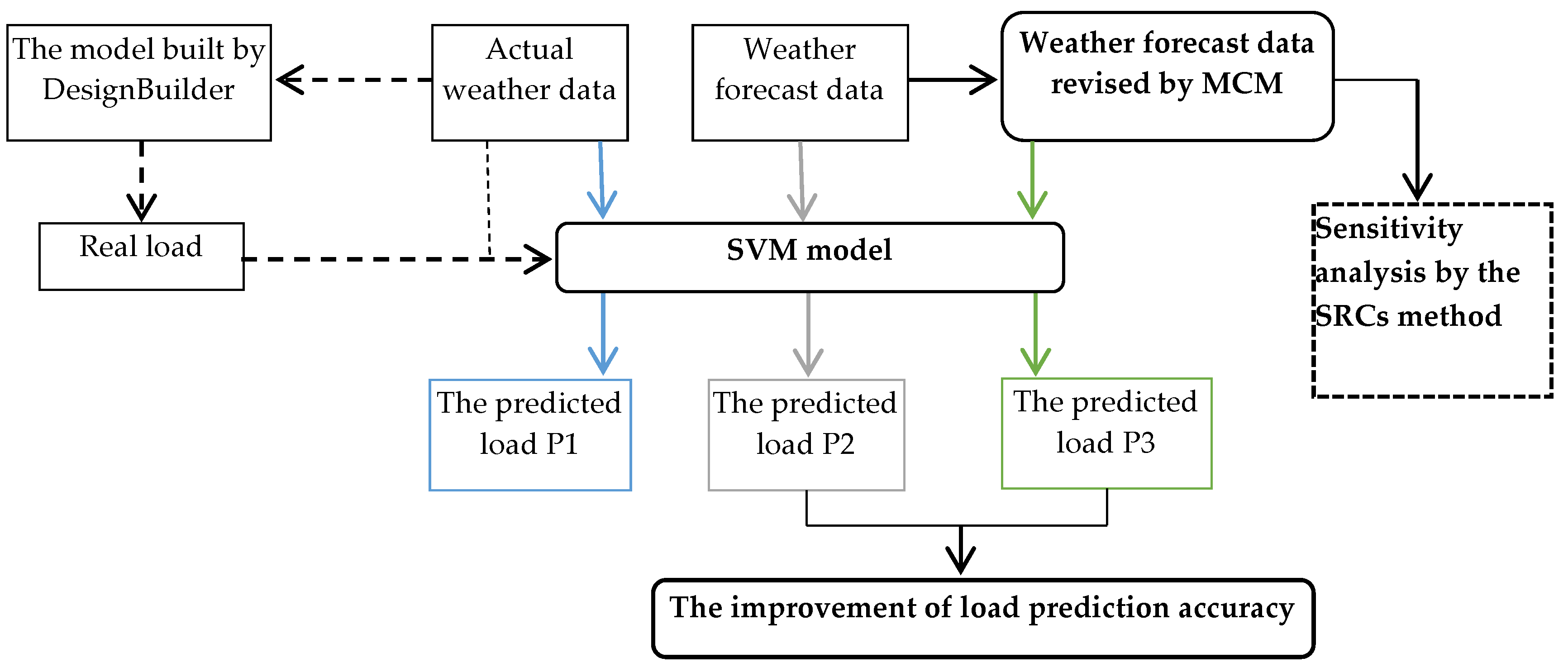
In this paper, the MCM is used to analyze the uncertainties of weather forecasting parameters, and the model based on SVM is established to forecast the cooling load of an office building. In addition, the Standardized Regression Coefficient (SRC) method for sensitivity analysis is introduced comprehensively. The flowchart shown in Figure 1 depicts the main steps in developing the research, which facilitates the understanding of the proposed approach.
2.1. The MCM of Random Sampling in Processing Weather Forecast Data
The MCM, also called a statistical simulation method, is an important numerical calculation method guided by probability statistics theory due to the development of science technology and the invention of electronic computers in the mid–1940s. It is an effective way to use random numbers to solve many problems. The Monte Carlo simulation is a method of studying the distribution characteristics by setting up a stochastic process and calculating the estimates and statistics of parameters. Specifically, the reliability of the system is too complex, and it is difficult to establish an accurate mathematical model for reliability prediction. When the model is inconvenient to apply, the estimated value of the desired target can be approximated by the stochastic simulation method. As the number of simulations increases, the expected accuracy of the target is gradually increased.
2.1.1. The Principle of the MCM
The Theorem of Large Numbers and Central Limits in Probability Theory are the theoretical basis of the MCM [25]. The principle of the Monte Carlo simulation method is that when the problem or the object itself has a probability feature, a sampling result can be generated by a computer simulation method. The statistic or the value of the parameter can be calculated according to the sampling.
Based on these two theorems, the function can be expressed as follows.
Assuming the function [26]:
where the probability distributions of the variables X1, X2, …, Xn are known. The values (x1, x2, …, xn) of each set of random variables (X1, X2, …, Xn) are obtained by direct or indirect sampling, then the value yi of the function Y can be determined according to Formula (2) [26]:
Sampling multiple times (i = 1, 2, …, m) repeatedly and independently, we can obtain a batch of sampling numbers y1, y2, …, yn of the function Y, which are in accordance with the characteristics of the normal distribution.
For each output, m possible results are obtained [20]:
2.1.2. The Steps of the MCM
First, a statistical analysis tool, such as IBM SPSS Statistics 19.0 software (19.0, IBM, Armonk, NY, USA), is used to analyze the probability distribution of the errors of the weather forecast data and the real data. A statistical model related to the problem is determined, of which the solution is regarded as the probability distribution and mathematical expectation of the constructed model. Generally, an appropriate theoretical distribution (e.g., Uniform distribution, Normal distribution, Binomial distribution, Poisson distribution, Triangular distribution, etc.) is used to describe the empirical probability distribution of random variables. If there is no typical theoretical probability distribution that can be directly quoted, it is necessary to estimate an initial probability distribution of the research object based on historical statistics and subjective prediction.
Second, it is important to generate random numbers to simulate the random changes of variables. There are mainly two methods to generate random numbers. We can use an existing random numbers table, or they can be calculated by using a computer program. In this paper, the program of the MCM for the research was written into MATLAB to implement the Monte Carlo random sampling according to the probability distribution obtained by the previous step. After multiple sampling, we can get m possible results, such as Equation (2).
Finally, when the number of simulations is sufficiently large, the probability distribution of the function Y and the concerned digital feature information can be close to the actual situation. Stable conclusions could be obtained by averaging the statistics or estimates of the parameters.
where yi (i = 1, 2, …, m) is the sampling result calculated by Equation (2). is the expected value of the results.
2.2. The Load Forecast Model Based on SVM
SVM is the technique first proposed by Vapnik to solve classification and regression problems [27]. SVR is a machine learning method based on statistical learning theory. It can effectively solve practical problems such as small samples and nonlinearities and has strong generalization ability. It mainly includes two regression models: ε-SVR and υ-SVR. The ε-SVR model is used in this paper. By introducing a kernel function, the nonlinear problem of low-dimensional space is transformed into a linear problem in high-dimensional feature space using nonlinear mapping. After the transformation, the decision function [28] is:
In Formula (5), ω is a weight vector, is a threshold, and is a sublinear mapping relationship from a low-dimensional space to a high-dimensional space.
The SVM uses the minimum structural risk to determine the parameters ω and b and introduces the insensitive loss function parameter ε, which translates the problem into the following optimization problems [28]:
where (x1, y1), …, (xm, ym) are a pair of input and output vectors, m is the number of samples, ω is weight factor, b is the threshold value, C is error cost, input samples are mapped to higher dimensional space by using kernel function φ, is the upper training error and the is the lower training error subject to ε-insensitive tube .
The SVM includes two parameters: Intrinsic parameters of the support vector machine, including the penalty parameter ‘C’, the loss function parameter ‘ε’; and parameters in the kernel function, such as the kernel width in the Gaussian kernel. The choices of these parameters are very important. The penalty parameter ‘C’ directly affects the complexity and stability of the model. It can make the model a tradeoff between complexity and training error. The loss function parameter ‘ε’ controls the simulation of SVR, which effects the number of support vectors and the generalization ability of the model. The width coefficient ‘γ’ in the kernel function that reflects the correlation between the vectors. The main types of kernel functions include linear kernel functions, polynomial kernel functions, Gaussian radial basis kernel functions, and sigmoid colony kernel functions. Among these functions, Gaussian kernel functions, suited to represent the complex nonlinear relationship between input and output [28,29], have the advantages of computational efficiency, simplicity, reliability, and ease of adaptation. Gaussian kernel functions [28] are as follows:
where the γ is the kernel parameter. When training SVM models, two free parameters need to be identified, which are kernel parameter γ and regularization constant C.
Since the key parameters of the above support vector machine model directly affect the accuracy of the model, this paper uses the particle swarm optimization algorithm to determine the optimal combination of these parameters, and then substitutes the optimal combination parameters into the support vector machine model to obtain its regression model. The specific steps are as follows:
- Data normalization:where are data before and after normalization, respectively, and and are the respective minimum and maximum values of the column where is located. The normalization process of the dependent variable data is similar to the independent variable data, and will not be described here.
- Establishing the support vector machine objective function based on training samples.
- Using the particle swarm optimization algorithm to select the key parameters of the SVM to obtain the optimal combination of the key parameters of the SVM.
- Substituting the optimal combination parameters into the SVM model to obtain its regression model.
- Using the prediction sample and the model obtained above to forecast the energy consumption of the building.
2.3. The SRCs Method for Sensitivity Analysis
Sensitivity analysis is used to study the mapping relations of uncertainties of input parameters and outputs [30]. There are a lot of sensitivity analysis methods among previous studies [31]. Some methods directly research the input-output map generated by the Monte Carlo method without additional runs of the model. Other methods propagate specific samples are aimed at the sensitivity analysis, for example, the screening method of Morris [32]. The SRCs method has been adopted in this paper, of which the basis is to fit a linear multidimensional model [20] between model inputs and model outputs.
The regression coefficients are determined such that the sum of error squares
is minimized. The following ratio, called the coefficient of determination [20],
is a measure of how well the model (12) matches the data. The closer to 1 the corresponding value of R2, the greater the model matches the data, but considering the different units and orders of magnitude of parameters, these drawbacks are easily worked out reformulating Equation (12) [20] as
where is the mean value and the variance of the output under the consideration
and is the mean value and the variance of the j input factor
Under the premise that the input variables are independent, the SRCs show the importance of each factor through moving each factor from its expected value by a fixed fraction of its standard deviation while keeping all other factors at their expected values [20]. Calculating the SRCs means to perform the regression analysis, with input and output parameters normalized to zero and standard deviation one. A positive sign indicates that the input is positively correlated with the output, while a negative sign indicates a negative correlation. The importance of these factors can be ranked according to the absolute value of the SRCs.
3. Case Study and Results
3.1. The Framework of the Case Study
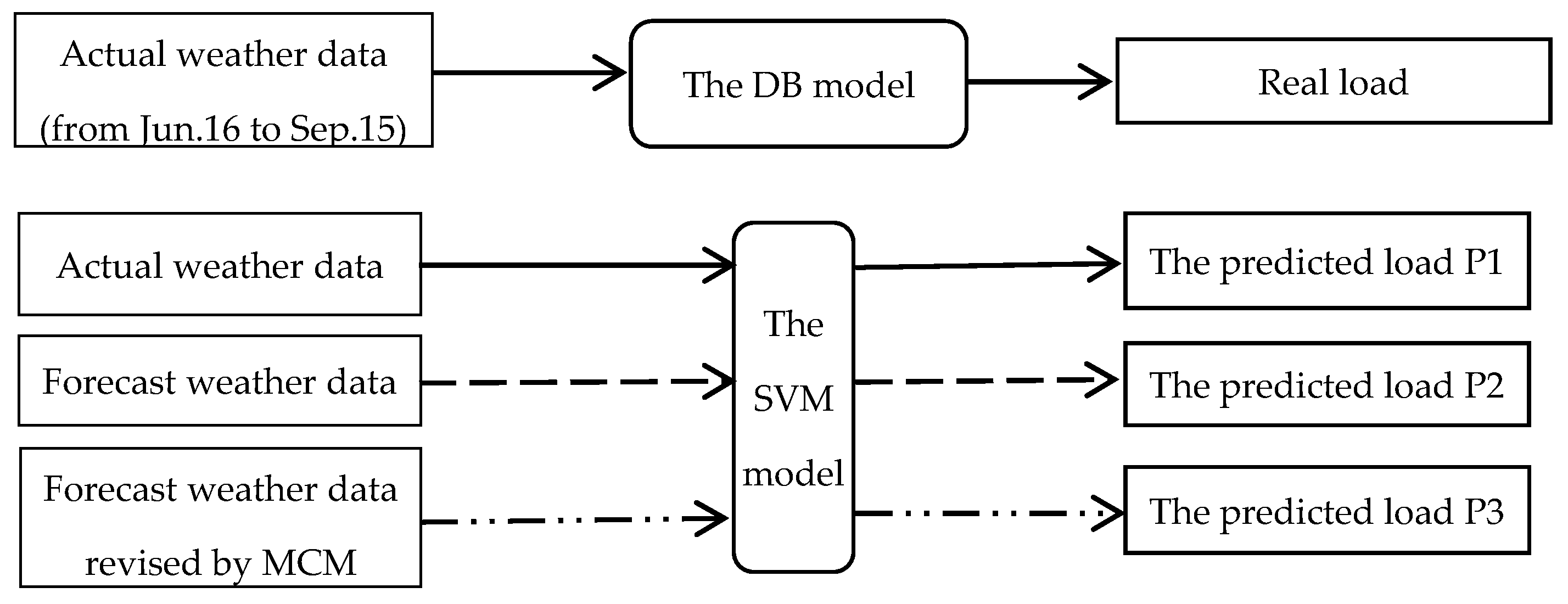
The framework of the case study is shown in Figure 2. The real-time meteorological parameters that we collected were input into the DesignBuilder (DB), and the simulated cooling load was regarded as the real load of the office building. Next, the actual meteorological data and simulated load data are used as training samples to build a load forecasting model based on SVM. We use the actual weather data in July as test samples to perform load forecasting to obtain the predicted load P1. Then, the weather forecast data before and after processing are input into the SVM model to obtain predicted loads P2 and P3, which are used for comparing the prediction accuracy of P2 and P3. Sensitivity analysis was used to study the factors that have a significant impact on load forecasting in the input parameters.
In order to verify the validity of the MCM and the SVM model established, three evaluation indexes are used to compare the prediction results between P1, P2 and P3, which include the following: the Mean Absolute Percentage Error (MAPE) [33], the Mean Absolute Error (MAE) [34], the Root Mean Square Error (RMSE) [34]. Their definitions and the calculation results can then be shown as follows.
where is the real load, is the forecasting load, and N is the number of samples.
MAPE not only considers the error between the predicted value and the true value but also the ratio between the error and the true value. It is a measure of the accuracy of the total prediction in the statistical field [32]. MAE and RMSE can amplify the value of the larger prediction bias, which can compare the stability of different prediction models.
3.2. Data Sources and Collection
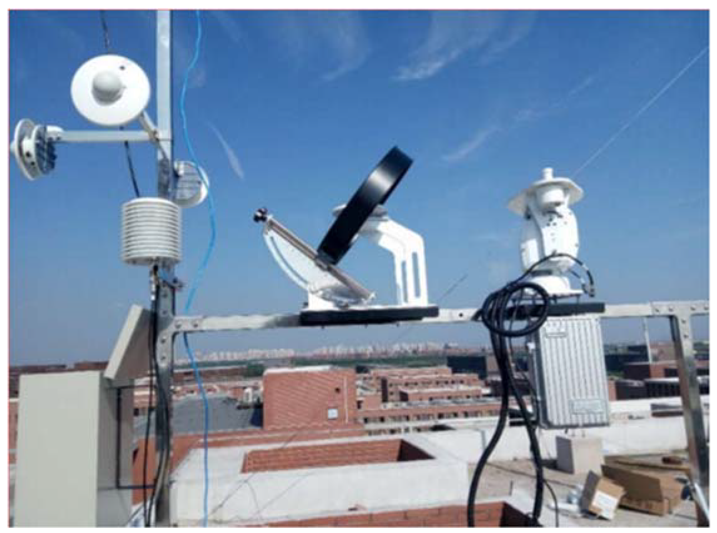
The data used in the research work of this paper mainly include two parts: meteorological data and load data. For the load forecasting work, there are mainly two ways to obtain the energy consumption of the construction. First, it is obtained through testing. In addition, it is calculated using energy simulation software. For the first approach, due to the low level of operation and management techniques of the current HVAC system, it is usually regulated by the operating experience of workers. The adjustment of the HVAC system has a certain lag, which cannot immediately bring changes to the load even if it is adjusted according to actual conditions. In the case of fluctuations of indoor temperature, the load data obtained by this method do not reflect the impact of real-time changes in meteorological parameters. Therefore, this paper adopts the second method. We use DesignBuilder to simulate the cooling load of the building, analyze the relevant data and establish the model. The meteorological data used in this paper are composed of real-time weather data collected by a small weather station shown in Figure 3 and weather forecast data from the weather website (https://www.worldweatheronline.com). Table 1 shows the measurement information of the weather elements recorded by the station.
This small weather station is located in Tianjin University, China, which consists of a PC-2-T solar radiation observer, a PC-4 meteorological monitoring recorder, transducers and the management software of the weather station monitoring system. It records the weather data every half hour by these devices and transfers data to the computer via wired cables. The weather data collected by the meteorological station mainly include dry-bulb temperature, relative humidity, wind speed, wind direction, sunshine hours, rainfall, solar radiation intensity. In addition, among the weather parameters from most existing weather websites, the prediction accuracies of the dry-bulb temperature and the relative humidity are relatively high, while the prediction accuracies of parameters such as wind speed, wind direction and solar radiation intensity are poor. Some cannot be predicted in advance, such as solar radiation intensity. Most of the previous literature selected temperature and relative humidity as inputs to establish the prediction model [14,15,16]. Therefore, in this paper, we mainly recorded the hourly weather forecast data from the weather website, including dry-bulb temperature and relative humidity, and discussed the influence of the uncertainty of forecast dry-bulb temperature and relative humidity on the cooling load forecast.
3.3. The DB Model of the Office Building
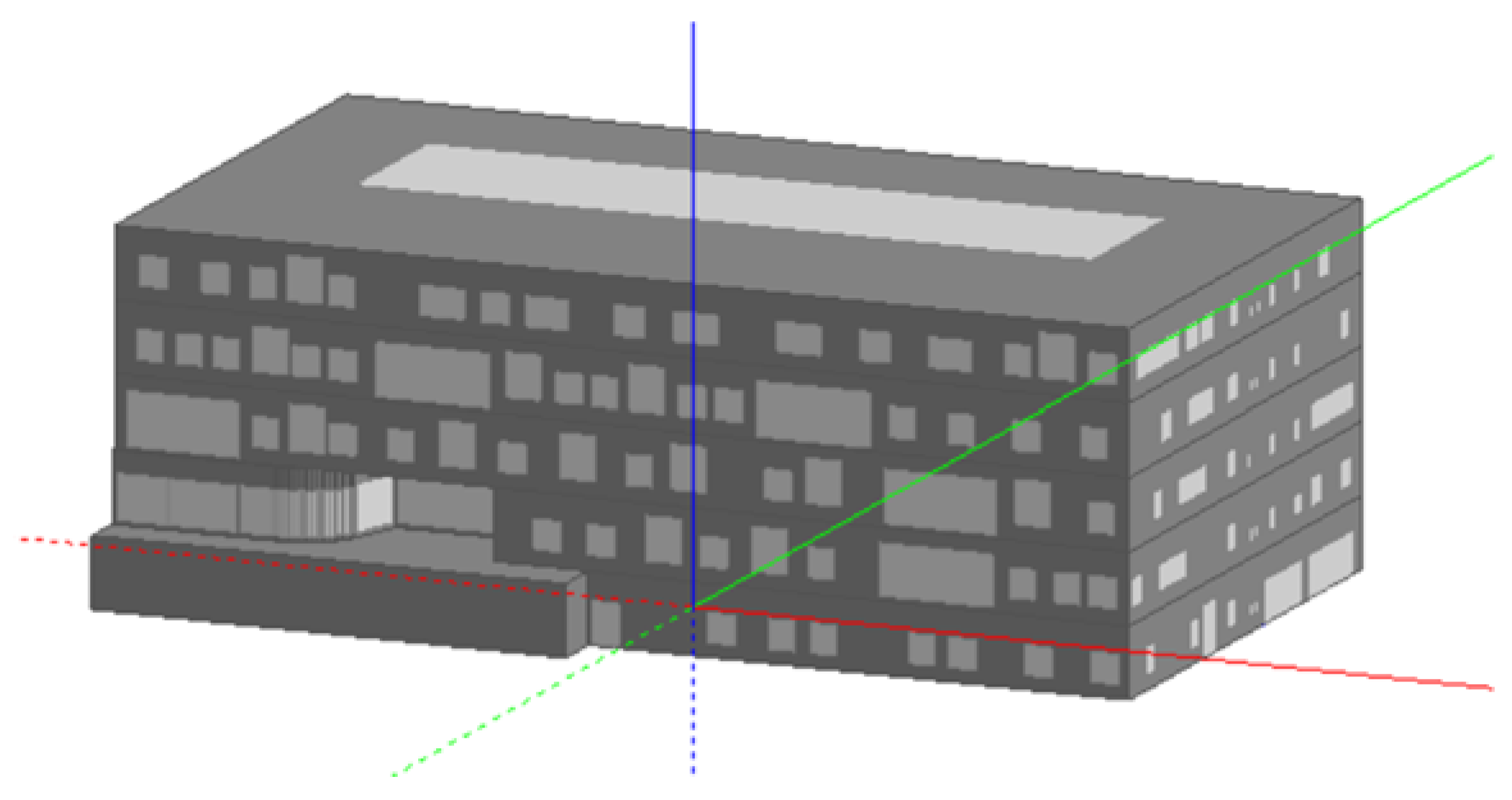
The case selected in this article is an office building in Tianjin City, located in Binhai New District, Tianjin, with a construction area of 10,723.16 square meters, building height of 22.80 m, 5 floors above ground, 1 floor underground and a roof set with skylights.
The final model created by the DesignBuilder software version 4.2.0.015 is shown in Figure 4. DB is the most comprehensive Graphical User Interface to the Energy Plus simulation engine which is widely used for modeling [35]. Parameters of the building structure are obtained through research, and other parameters refer to “Tianjin Public Building Energy Efficiency Design Standards” (DB 29-153-2014) for setting, such as personnel density, personnel per room rate, lighting density, running time. The heat source is supplied by the district heating pipe network in winter, and the terminal of the air conditioning system is the fan coil system, while it uses the split Variable Refrigerant Volume (VRV) air conditioning system for cooling in summer. It is difficult to obtain the hourly cooling load by measurement. In addition, the HVAC systems of the office building are normally used from Monday to Friday and are not used on weekends and holidays. Therefore, only the loads from 9 a.m. to 5 p.m. on weekdays are considered in the scope of the study of load forecasting. The error analysis of the simulated hourly heating load and the measured heating supply data from 9:00 to 17:00 for three working days is carried out to verify the simulation.
The result is shown in Figure 5. The average relative error between the measured data and the simulated data was 16.1%, which is acceptable considering of the limitations of the on-site tests and measurement instruments. Therefore, the simulation load can be regarded as the real load to establish the database.
3.4. The SVM Model and Validation
The final input parameters of the dynamic cooling load forecasting model for the construction of this project still need to be determined in combination with the weather forecast and the actual situation. For the 24-h-ahead load forecasting model, it is difficult to obtain information about historical loads and solar radiation values for the 1-h to 3-h ahead, so we select weather data and load data from 16 June to 15 September as training samples (576 observation values) to establish a support vector machine model. Table 2 gives some examples of training samples.
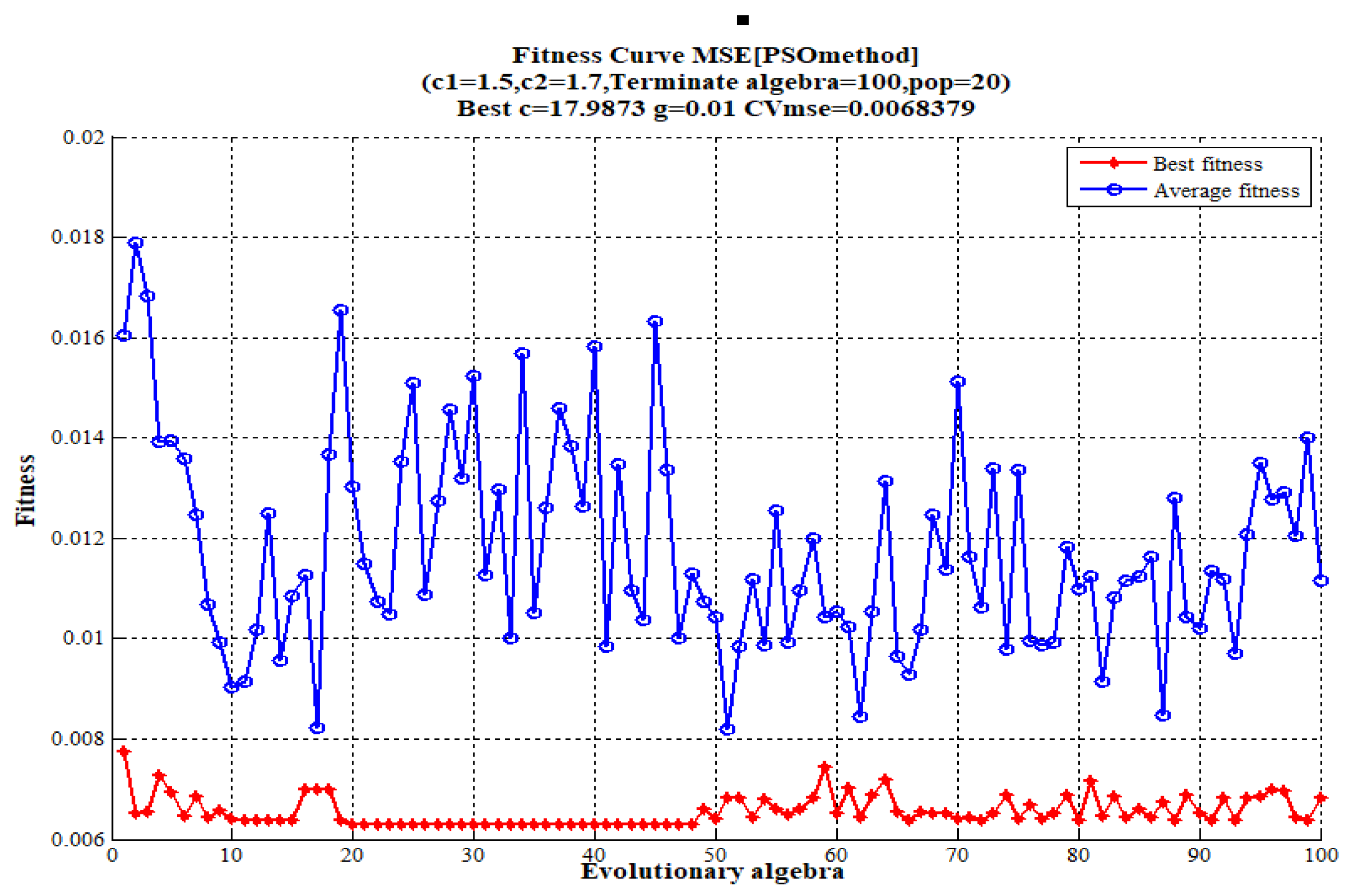
The particle swarm optimization algorithm is used to optimize the parameters of the support vector machine, where we set , where g is γ in Equation (10). The particle swarm optimization algorithm hyper-parameter optimization results are: . Figure 6 shows the results of the fitness function of the particle swarm optimization algorithm.
According to the above optimal parameter combination, the cooling load forecasting model based on SVM can be obtained. We use the actual meteorological parameters in July as test samples. Then, the forecasted data are anti-normalized to obtain the load forecast value, which is compared with the actual load simulated by DesignBuilder to verify the accuracy of the SVM model. The results of the comparison are shown in Figure 7.
By calculation, the MAPE of the SVM model is 10.74% compared to the actual situation. Due to the 24-h-ahead load forecast model and the source limits of weather forecast data, we believe that the model basically meets the forecasting requirements. The next research can be done using this model.
3.5. Load Prediction with the Weather Forecast Data
3.5.1. Data Preprocessing Based on MCM
We recorded daily weather forecast data for July except for weekends with a total of 171 samples. Through analysis, it is found that the errors between weather forecast data and real weather data obey the normal distribution . In order to study the influence of the uncertainty of the weather forecast data on the accuracy of load forecasting, we use the MCM to modify the input parameters of the SVM model, namely, the meteorological data. Then, the preprocessed weather forecast data are input into the model for load forecasting.
The IBM SPSS Statistics 19.0 software is used to analyze the error distribution of seven meteorological input parameters in turn. Figure 8 shows the error probability distribution between the weather forecast temperature T(h–1) and the actual temperature one hour before the predicted time. The mean value is and the standard deviation is .
Next, we write the program of MCM into MATLAB to implement the Monte Carlo random sampling of its error , setting the number of simulations M as 1000, and use a corresponding calculation program to obtain a set of revised weather forecast data T(h–1)*. The formula is as follows:
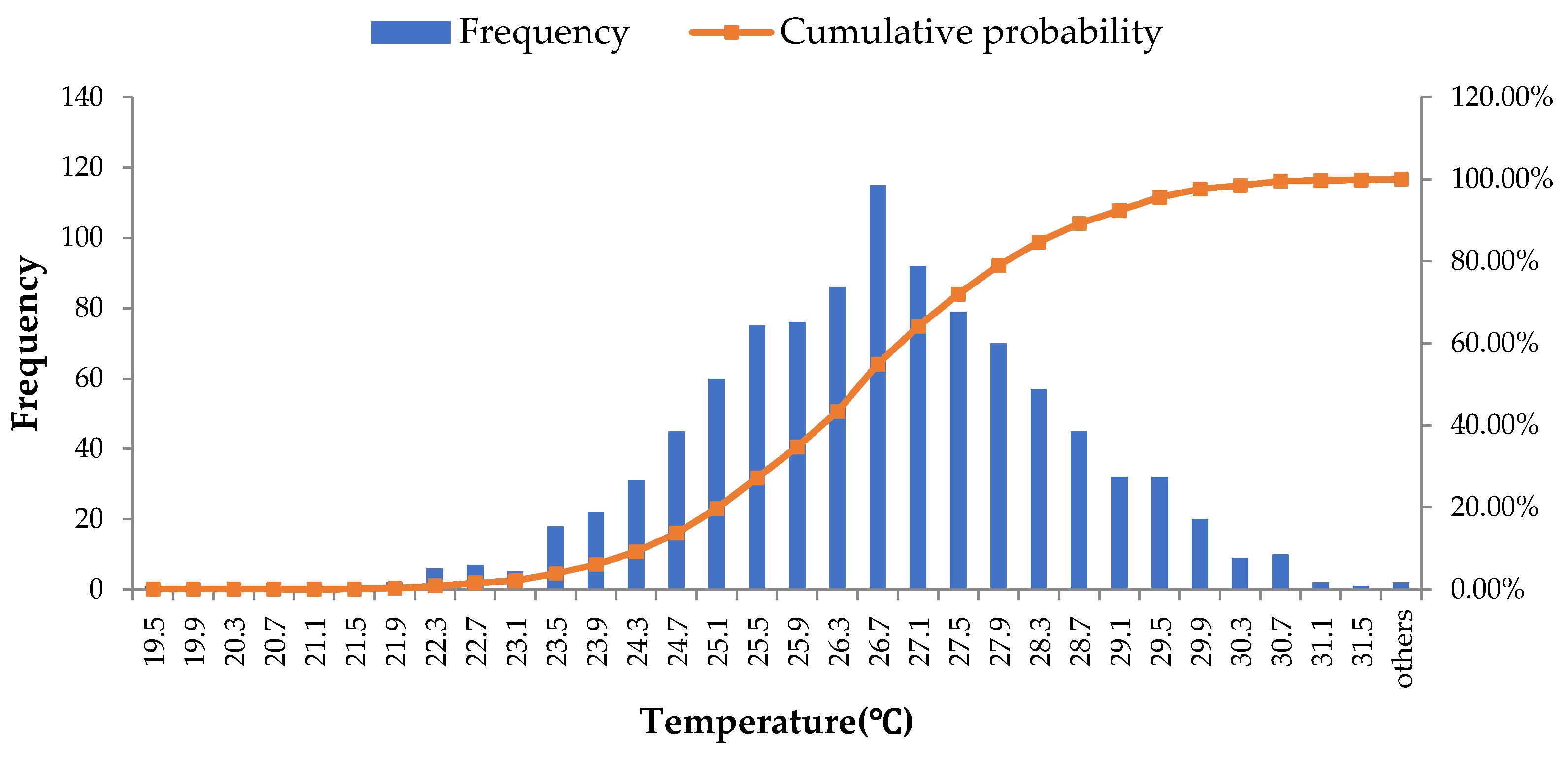
For example, for forecasting the load at 9 o’clock on 3 July, it is known that the 1-h-ahead weather forecast dry bulb temperature of the prediction moment T(h–1) is 27.2 °C. The result of the random sampling for T(h–1) using the MCM based on 1000 runs of the model is shown in Figure 9. The most frequent values of T(h–1) in the results of random sampling simulation are near 26.7 °C. Actually, the error ∆w obtained by random sampling is −0.6 through calculation, and the revised weather forecast data T(h–1)* is 26.6 °C, which means that the expected value of T(h–1) is 26.6 °C and is closer to the real weather data, i.e., 26.0 °C.
Table 3 lists the example of the corrected weather forecast values using MCM and actual values to predict the cooling load at 9 o’clock on 3 July. It can be seen that the weather forecast data corrected by MCM are closer to the actual data. The other samples have the same effects and will not be repeated here due to space limitations.
Table 4 shows the probability distribution functions obeyed by the errors of input parameters obtained from the statistical analysis by SPSS. The procedures for the correction of other parameters are similar to that of the parameter T(h–1). We no longer describe more details here.
We imported the forecast data for July before and after the correction into the SVM model for load forecasting. Both of the results are compared with the real cooling load simulated by the DesignBuilder, which are shown in Figure 10.
As can be seen from the figures above, the prediction results of P2 and P3 are still different from the actual load at some points, but P3 is closer to the real load from the overall level than P2, especially from 10th to 24th July. This proves that the uncertainty analysis of weather forecast data for cooling load forecasting based on MCM is beneficial to improve the accuracy of load prediction.
According to the results of load forecasting under the two scenarios, the evaluation of the prediction performance is shown in Table 5. As can be seen from the table, the 24-h-ahead load forecasting model based on SVM has good prediction accuracy. We established the SVM model and used actual meteorological data for load forecasting. The MAPE of P1 compared with the actual load is 10.74%, which includes the uncertainty of the model itself. Then, using the weather forecast data before and after processing with MCM to forecast load separately, we obtain the forecast results P2 and P3. The accuracy of load forecasting using the meteorological forecast data directly and that of the data processed by the MCM are 11.54%, 10.92%, respectively. In terms of MAE and RMSE, the values of P2 are 74.3807 kW and 90.8474 kW, respectively, while the values of P3 are 67.0291 kW and 85.4057 kW. It is clear that the accuracy of P3 is better than that of P2.
3.5.2. Sensitivity Analysis
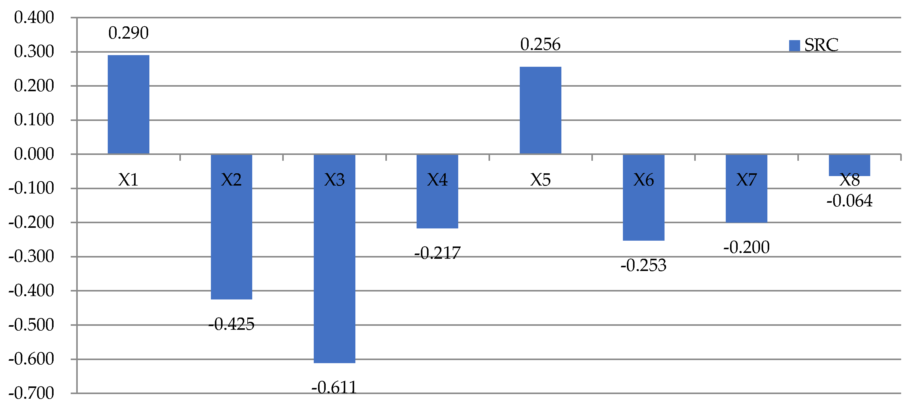
The SRCs for the case study are shown in Figure 11. The uncertainty in the previous seven factors explains most of the variance in the cooling load forecasting that is observed in Figure 10b. The remaining one uncertain factor RH(h–2) has little or no effect on the load forecasting.
It can be found that from the input parameters we selected, the factors that have the greatest impact on the load forecast are T(h–1) > T(h) > L(d–1, h) > T(h–3) > RH(h) > T(h–2) > RH(h–1) > RH(h–2) in turn. Obviously, the load at the predicted moment is mostly affected by the outdoor temperature at the previous moment. Due to the thermal inertia of the enclosure, the disturbance caused by the change of the outdoor temperature will not immediately affect the indoor temperature. Heat is transferred between the envelopes with detention and attenuation, which affects the load of the building in the next moments.
4. Discussion
Overviewing the previous research in Section 1, most focused on the optimization of the load prediction model itself to improve the accuracy of load prediction, and few studies have paid attention to the influence of uncertainty of the weather forecast data on the load forecasting. This paper fills a gap in this aspect by uncertainty analysis of weather forecast data for cooling load forecasting based on MCM. Three evaluation indexes are used to compare the prediction results between P1, P2 and P3 in Section 3.4. The results illustrate that the evaluation of the load forecasting with the data processed by the MCM is better than that of the load forecasting using the meteorological forecast data directly according to Figure 10 and Table 5. Furthermore, through sensitivity analysis, it was found that among the selected weather parameters shown in Figure 11, the factor that had the greatest impact on the prediction results was the 1-h-ahead temperature T(h–1) at the prediction moment.
It is worth noting that both of the results P2 and P3 are obtained by the SVM model, and their uncertainties include two parts: one is the uncertainty from the SVM model itself, and the other is the uncertainty from the weather forecast data. This paper mainly focuses on adopting the MCM to process weather forecast data and explore the impact of the uncertainty of weather forecast on load forecasting, not the load forecasting model itself. The research just selects the SVM model as an example, because it is accepted by most researchers due to good performance. With the development of artificial intelligence algorithm technology, the optimal combination of various algorithms is used for load prediction [35], which indicates that the accuracy of load forecasting model itself can be improved to some extent.
The data-preprocessing method based on MCM makes the forecasting results closer to the actual load compared to those without processing, which is suitable for not only office buildings but also other types of buildings. The precise load forecasting results are conducive to the HVAC system operation control. Moreover, the MCM method is convenient for application. Historical weather forecast data and real-time meteorological data are obtained from reliable weather forecasting agencies. In addition, SPSS is used to analyze and obtain the probability distributions of the errors between weather forecast data and real-time meteorological data. The revised weather data are obtained by MATLAB with the relevant programs according to the probability distribution of the errors. Both of the tools are free for application.
When using the MCM to process weather forecast data, it is necessary to analyze the probability distribution characteristics that the error between the weather forecast data and actual weather data obey. The current work is limited by the sources of historical weather forecast data. The larger the historical samples size we collect from the weather forecast websites, the more accurate the probability distribution function of the errors, and then the closer the modified weather forecast data to the actual weather data. In the future, under the condition that the meteorological forecast data sources are more widely available and reliable, the 1-h-ahead load forecasting model can be established to predict the load combined with the MCM for data processing. It seems that more precise results of load predictions will be obtained. With the completion of follow-up work, software of the data-preprocessing method based on MCM will be developed.
5. Conclusions
This paper investigated the influence of the uncertainty of weather forecast data on the cooling load forecast. Here, taking the 24-h-ahead SVM model as an example, the MCM was adopted to preprocess meteorological forecast data to improve the accuracy of load forecasting. It was indicated that the accuracy of the load forecasting with the data processed by the MCM is better than that of the load forecasting using the meteorological forecast data directly, which is closer to the real load.
Among the selected input parameters, the factors that have the greatest impact on the load forecast are T(h–1) >T(h) > L(d–1, h) > T(h–3) > RH(h) > T(h–2) > RH(h–1) >RH(h–2) in turn. Therefore, we must improve the accuracy of model input parameters to reduce the influence of uncertainty deriving from input parameters on load forecasting, especially those influential input parameters.
Author Contributions
Conceptualization, J.Z. and Y.D.; Methodology, J.Z. and Y.D.; Software, Y.D. and X.L.; Validation, Y.D. and X.L.; Formal Analysis, Y.D.; Writing—Original Draft Preparation, Y.D. and X.L.; Writing—Review & Editing, J.Z. and Y.D.
Funding
This research was funded by the Natural Science Foundation of China, grant number [51508380].
Conflicts of Interest
The authors declare no conflict of interest.
References
- Verhelst, J.; Van, H.G.; Saelens, D. Model selection for continuous commissioning of HVAC-systems in office buildings: A review. Renew. Sustain. Energy Rev. 2017, 76, 673–686. [Google Scholar] [CrossRef]
- Xia, C.H.; Xiang, X.J.; Hu, X.Y. Design of virtual instrument for load forecasting based on RBF neural network and weather data. Relay 2007, 35, 29–32. [Google Scholar]
- Ruzic, S.; Vuckovic, A.; Nikolic, N. Weather sensitive method for short term load forecasting in Electric Power Utility of Serbia. IEEE Trans. Power Syst. 2003, 18, 1581–1586. [Google Scholar] [CrossRef]
- Wi, Y.M.; Joo, S.K.; Songk, K.B. Holiday load forecasting using fuzzy polynomial regression with weather feature selection and adjustment. IEEE Trans. Power Syst. 2012, 27, 596–603. [Google Scholar] [CrossRef]
- Cao, L. Support vector machines experts for time series forecasting. Neurocomputing 2003, 51, 321–339. [Google Scholar] [CrossRef] [Green Version]
- Huang, W.; Nakamori, Y.; Wang, S.Y. Forecasting stock market movement direction with support vector machine. Comput. Oper. Res. 2005, 32, 2513–2522. [Google Scholar] [CrossRef]
- Pai, P.F.; Lin, C.S. A hybrid ARIMA and support vector machines model in stock price forecasting. Omega 2005, 33, 497–505. [Google Scholar] [CrossRef]
- Pai, P.F.; Hong, W.C. Software reliability forecasting by support vector machines with simulated annealing algorithms. J. Syst. Softw. 2006, 79, 747–755. [Google Scholar] [CrossRef]
- Mohandes, M.A.; Halawani, T.O.; Rehman, S.; Hussain, A.A. Support vector machines for wind speed prediction. Renew. Energy 2004, 29, 939–947. [Google Scholar] [CrossRef]
- Amari, S.; Wu, S. Improving support vector machine classiers by modifying kernel functions. Neural Netw. 1999, 12, 783–789. [Google Scholar] [CrossRef]
- Cherkassky, V.; Ma, Y. Practical selection of SVM parameters and noise estimation for SVM regression. Neural Netw. 2004, 17, 113–126. [Google Scholar] [CrossRef] [Green Version]
- Barman, M.; Choudhury, N.B.D.; Sutradhar, S. A regional hybrid GOA-SVM model based on similar day approach for short-term load forecasting in Assam, India. Energy 2018, 145, 710–720. [Google Scholar] [CrossRef]
- Li, X.; Shao, M.; Ding, L.; Xu, G. Particle swarm optimization-based LS-SVM for building cooling load prediction. J. Comput. 2010, 5, 614–621. [Google Scholar] [CrossRef]
- Duanmu, L.; Wang, Z.; Zhai, Z.J. A simplified method to predict hourly building cooling load for urban energy planning. Energy Build. 2013, 58, 281–291. [Google Scholar] [CrossRef]
- Wang, H.; Chen, Q.; Ren, Z. Impact of climate change heating and cooling energy use in buildings in the United States. Energy Build. 2014, 82, 428–436. [Google Scholar] [CrossRef]
- Jiang, Y. Generation of typical meteorological year for different climates of China. Energy 2010, 35, 1946–1953. [Google Scholar] [CrossRef]
- Chen, D.; Wang, X.; Ren, Z. Selection of climatic variables and time scales for future weather preparation in building heating and cooling energy predictions. Energy Build. 2012, 51, 223–233. [Google Scholar] [CrossRef]
- Petersen, S.; Bundgaard, K.W. The effect of weather forecast uncertainty on a predictive control concept for building systems operation. Appl. Energy 2014, 116, 311–321. [Google Scholar] [CrossRef]
- Eua-Arporn, B.; Yokoyama, A. Short-term operating strategy with consideration of load forecast and generating unit uncertainty. IEEJ Trans. Power Energy 2007, 127, 1159–1167. [Google Scholar] [CrossRef]
- Domínguez-Muñoz, F.; Cejudo-López, J.M.; Carrillo-Andrés, A. Uncertainty in peak cooling load calculations. Energy Build. 2010, 42, 1010–1018. [Google Scholar] [CrossRef]
- Douglas, A.P.; Breipohl, A.M.; Lee, F.N.; Adapa, R. The impacts of temperature forecast uncertainty on Bayesian load forecasting. IEEE Trans. Power Syst. 1998, 13, 1507–1513. [Google Scholar] [CrossRef]
- MacDonald, I. Quantifying the Effects of Uncertainty in Building Simulation. Ph.D Thesis, Department of Mechanical Engineering, University of Strathclyde, Glasgow, UK, 2002. [Google Scholar]
- Domínguez-Muñoz, F.; Anderson, B.; Cejudo-López, J.M.; Carrillo-Andrés, A. Uncertainty in the thermal conductivity of insulation materials. In Proceedings of the Eleventh International IBPSA Conference, Glasgow, UK, 27–30 July 2009. [Google Scholar]
- Sten, D.W.; Augenbroe, G. Analysis of uncertainty in building design evaluations and its implications. Energy Build. 2002, 34, 951–958. [Google Scholar]
- Reiter, D. The Monte Carlo Method, an Introduction. Lect. Notes Phys. 2008, 50, 63–78. [Google Scholar]
- Papadopoulos, C.E.; Yeung, H. Uncertainty estimation and Monte Carlo simulation method. Flow Meas. Instrum. 2002, 12, 291–298. [Google Scholar] [CrossRef]
- Selakov, A.; Cvijetinović, D.; Milović, L. Hybrid PSO-SVM method for short-term load forecasting during periods with significant temperature variations in city of Burbank. Appl. Soft Comput. 2014, 16, 80–88. [Google Scholar] [CrossRef]
- Fu, Y.; Li, Z.; Zhang, H. Using Support vector machine to predict next-day electricity load of public buildings with sub-metering devices. Procedia Eng. 2015, 121, 1016–1022. [Google Scholar] [CrossRef]
- Ebtehaj, I.; Bonakdari, H.; Shamshirband, S. A combined support vector machine-wavelet transform model for prediction of sediment transport in sewer. Flow Meas. Instrum. 2016, 47, 19–27. [Google Scholar] [CrossRef]
- Saltelli, A.; Tarantola, S.; Campolongo, F.; Ratto, M. Sensitivity Analysis in Practice. J. Am. Stat. Assoc. 1989, 101, 398–399. [Google Scholar]
- Saltelli, A.; Chan, K.; Scott, E.M. Sensitivity Analysis: Gauging the Worth of Scientific Models; John Wiley and Sons: Chichester, UK, 2000. [Google Scholar]
- Morris, M.D. Factorial sampling plans for preliminary computational experiments. Technometrics 1991, 33, 161–174. [Google Scholar] [CrossRef]
- Tayman, J.; Swanson, D.A. On the validity of MAPE as a measure of population forecast accuracy. Popul. Res. Policy Rev. 1999, 18, 299–322. [Google Scholar] [CrossRef]
- Zhao, J.; Liu, X.J. A hybrid method of dynamic cooling and heating load forecasting for office buildings based on artificial intelligence and regression analysis. Energy Build. 2018. [Google Scholar] [CrossRef]
- Iman, W.; Mohd, W.; Royapoor, M.; Wang, Y.; Roskilly, A.P. Office building cooling load reduction using thermal analysis method-A case study. Appl. Energy 2017, 185, 1574–1584. [Google Scholar]
Figure 1.
The framework of the research methods.

Figure 2.
The framework of the case study.

Figure 3.
Meteorological station.

Figure 4.
The office building model built by DesignBuilder.

Figure 5.
Comparison between the simulated heating load and the measured heating supply.

Figure 6.
The fitness curve of the particle swarm optimization algorithm.

Figure 7.
Comparison between the real load and forecast load P1. P1 is the forecast load adopting real weather data using the SVM model.
Figure 7.
Comparison between the real load and forecast load P1. P1 is the forecast load adopting real weather data using the SVM model.

Figure 8.
The error probability distribution of T(h–1).

Figure 9.
Histogram and the cumulative probability distribution of the T(h–1)*.

Figure 10.
In (a), P2 is the forecasting load adopting weather forecast data, and in (b), P3 is the forecasting load adopting the weather forecast data dealt with MCM.
Figure 10.
In (a), P2 is the forecasting load adopting weather forecast data, and in (b), P3 is the forecasting load adopting the weather forecast data dealt with MCM.

Figure 11.
The SRCs of input parameters of the case study. X1 = L(d–1, h); X2 = T(h);X3 = T(h–1); X4 = T(h–2); X5 = T(h–3); X6 = RH(h); X7 = RH(h–1); X8 = RH(h–2).
Figure 11.
The SRCs of input parameters of the case study. X1 = L(d–1, h); X2 = T(h);X3 = T(h–1); X4 = T(h–2); X5 = T(h–3); X6 = RH(h); X7 = RH(h–1); X8 = RH(h–2).


Table 1.
Measurement information of the meteorological elements.
| Meteorological Element | Measuring Range | Resolution Ratio | Accuracy |
|---|---|---|---|
| Dry-bulb temperature | −50~+100 °C | 0.1 °C | ±0.2 °C |
| Relative humidity | 0~100% | 0.1% | ±2% (≤80%) ±5% (>80%) |
Table 2.
Some examples of training samples.
| Time | Output | Inputs | |||||||
|---|---|---|---|---|---|---|---|---|---|
| L(h) | L(d–1,h) | T(h) | T(h–1) | T(h–2) | T(h–3) | RH(h) | RH(h–1) | RH(h–2) | |
| 7/3/9:00 | −772.61 | −584.99 | 27.4 | 26.0 | 25.2 | 24.7 | 78.9 | 84.2 | 87.8 |
| 7/3/10:00 | −813.45 | −649.59 | 28.3 | 27.4 | 26.0 | 25.2 | 75.1 | 78.9 | 84.2 |
| 7/3/11:00 | −861.98 | −700.47 | 28.3 | 28.3 | 27.4 | 26.0 | 74.3 | 75.1 | 78.9 |
| 7/3/12:00 | −770.72 | −660.08 | 28.5 | 28.3 | 28.3 | 27.4 | 71.8 | 74.3 | 75.1 |
| 7/3/13:00 | −753.09 | −723.44 | 28.8 | 28.5 | 28.3 | 28.3 | 71.3 | 71.8 | 74.3 |
| 7/3/14:00 | −881.99 | −876.29 | 29.3 | 28.8 | 28.5 | 28.3 | 68.2 | 71.3 | 71.8 |
| 7/3/15:00 | −884.55 | −844.72 | 29.2 | 29.3 | 28.8 | 28.5 | 68.6 | 68.2 | 71.3 |
| 7/3/16:00 | −866.96 | −824.41 | 28.8 | 29.2 | 29.3 | 28.8 | 69.2 | 68.6 | 68.2 |
| 7/3/17:00 | −829.87 | −815.52 | 28.5 | 28.8 | 29.2 | 29.3 | 70.2 | 69.2 | 68.6 |
L(d–1, h) represents the historical load at the same moment we predict for the previous day. T(h), T(h–1), T(h–2), T(h–3) are the dry-bulb temperature at the moment we forecast and the time of the 1–h to 3–h ahead, respectively, RH(h), RH(h–1), RH(h–2) are the relative humidity at the moment we forecast and the 1–h to 2–h ahead, respectively.
Table 3.
The input parameters of the load forecasting model.
| Data Type | L(d–1,h) kw | T(h) °C | T(h–1) °C | T(h–2) °C | T(h–3) °C | RH(h) % | RH(h–1) % | RH(h–2) % |
|---|---|---|---|---|---|---|---|---|
| Actual data | −584.99 | 27.4 | 26.0 | 25.2 | 24.7 | 78.9 | 84.0 | 87.8 |
| Forecast data | −584.99 | 28.9 | 27.2 | 25.6 | 24.4 | 58.0 | 66.0 | 78.0 |
| Revised data | −584.99 | 28.2 | 26.6 | 25.1 | 24.1 | 68.0 | 75.1 | 86.0 |
Table 4.
The probability distribution of each input parameter.
| Factor | Parameter | Probability Distribution |
|---|---|---|
| X2 | T(h) | |
| X3 | T(h–1) | |
| X4 | T(h–2) | |
| X5 | T(h–3) | |
| X6 | RH(h) | |
| X7 | RH(h–1) | |
| X8 | RH(h–2) |
Table 5.
Comparison between P1, P2, and P3.
| Prediction Load | MAPE (%) | MAE (kW) | RMSE (kW) |
|---|---|---|---|
| P1 | 10.74% | 67.8305 | 84.4138 |
| P2 | 11.54% | 74.3807 | 90.8474 |
| P3 | 10.92% | 67.0291 | 85.4057 |
© 2018 by the authors. Licensee MDPI, Basel, Switzerland. This article is an open access article distributed under the terms and conditions of the Creative Commons Attribution (CC BY) license (http://creativecommons.org/licenses/by/4.0/).
Share and Cite
MDPI and ACS Style
Zhao, J.; Duan, Y.; Liu, X. Uncertainty Analysis of Weather Forecast Data for Cooling Load Forecasting Based on the Monte Carlo Method. Energies 2018, 11, 1900. https://doi.org/10.3390/en11071900
AMA Style
Zhao J, Duan Y, Liu X. Uncertainty Analysis of Weather Forecast Data for Cooling Load Forecasting Based on the Monte Carlo Method. Energies. 2018; 11(7):1900. https://doi.org/10.3390/en11071900
Chicago/Turabian StyleZhao, Jing, Yaoqi Duan, and Xiaojuan Liu. 2018. "Uncertainty Analysis of Weather Forecast Data for Cooling Load Forecasting Based on the Monte Carlo Method" Energies 11, no. 7: 1900. https://doi.org/10.3390/en11071900
Note that from the first issue of 2016, this journal uses article numbers instead of page numbers. See further details here.