Exploiting Artificial Neural Networks for the Prediction of Ancillary Energy Market Prices


1
Department of Electrical Engineering and Automation, School of Electrical Engineering, Aalto University, FI-00076 Espoo, Finland
2
National Institute of Informatics, Tokyo 100-0003, Japan
3
SRT, Luleå University of Technology, Luleå 97187, Sweden
4
International Research Laboratory of Computer Technologies, ITMO University, St. Petersburgh 197101, Russia
*
Author to whom correspondence should be addressed.
Energies 2018, 11(7), 1906; https://doi.org/10.3390/en11071906
Submission received: 28 June 2018
/
Revised: 17 July 2018
/
Accepted: 20 July 2018
/
Published: 21 July 2018
(This article belongs to the Collection Smart Grid)
Abstract
:The increase of distributed energy resources in the smart grid calls for new ways to profitably exploit these resources, which can participate in day-ahead ancillary energy markets by providing flexibility. Higher profits are available for resource owners that are able to anticipate price peaks and hours of low prices or zero prices, as well as to control the resource in such a way that exploits the price fluctuations. Thus, this study presents a solution in which artificial neural networks are exploited to predict the day-ahead ancillary energy market prices. The study employs the frequency containment reserve for the normal operations market as a case study and presents the methodology utilized for the prediction of the case study ancillary market prices. The relevant data sources for predicting the market prices are identified, then the frequency containment reserve market prices are analyzed and compared with the spot market prices. In addition, the methodology describes the choices behind the definition of the model validation method and the performance evaluation coefficient utilized in the study. Moreover, the empirical processes for designing an artificial neural network model are presented. The performance of the artificial neural network model is evaluated in detail by means of several experiments, showing robustness and adaptiveness to the fast-changing price behaviors. Finally, the developed artificial neural network model is shown to have better performance than two state of the art models, support vector regression and ARIMA, respectively.
1. Introduction
The emergence of the smart grid has resulted in the development of numerous smart Distributed Energy Resources (DER) such as battery storage, adjustable loads and electric vehicles with two-way charging capability. There are several possible ways to exploit these resources profitably. Some of these involve the use of the resources to reduce electricity bills, and comparing the profitability of these approaches can be straightforward, especially if experiments are performed in the same region and a fixed electricity price is used. However, the flexible capacity of the resources can also be traded on various markets, in which case the owner of the resource is required to enter into some business relationship with a party that is willing to pay for the possibility of using the resource. One possibility is that the owner participates in markets such as ancillary services. Alternatively, the owner can make an agreement with an aggregator [1] that will participate in the market on his/her behalf.
Several works published in leading journals have addressed this problem, but on a limited scale, so it is unclear how the research could be exploited for financial gain on existing or emerging electricity markets. For example, in [2], the authors did not choose any existing market, but proposed a negotiation scheme between the DER owner and the grid operator, effectively designing a new market, so the contribution of the research was to optimize the profits of the DER owner on that market. In [3], it was assumed that the electricity price was a linear function of the instant load. While [4] discussed an EV charging station for peak load shifting, no market mechanism for getting compensation from the grid operator was identified; nor did the intelligent control consider the possibilities of exploiting the differences in hourly electricity prices.
Several solutions have been proposed for using DERs to reduce electricity bills, in which case the DER owner does not need to participate in any market. Costs related to peak consumption can be effectively reduced with Vehicle-to-Home (V2H) [5] and Vehicle-to-Building (V2B) [6] technologies. V2H and V2B can also be used to exploit excess local energy production such as photovoltaic or wind power generation without selling it to the grid [7,8]. Various smart loads such as heat pumps [9] and electric vehicles [10,11] can be rescheduled to exploit low hourly electricity prices. In some cases, the use of DERs for Demand Response (DR) involves scheduling the energy consumption to exploit hourly differences in utility electricity prices [7], as well as the minimization of the costs for the power system [12]. In addition, various forms of DR involving DER are possible [13], such as the participation in ancillary services markets such as frequency control reserves [14].
Several works have addressed the problem of controlling DERs to meet the technical requirements to participate in ancillary services [15,16,17,18] and frequency control reserves in particular [19,20], but they did not attempt to quantify the financial benefit. In [21], an advanced bidding strategy on ancillary markets was presented that nevertheless did not exploit the predictions of ancillary market prices. Obviously, further work inspired by these articles would involve cost-benefit assessments of the proposed approaches and strategies to optimize the financial benefit as in [22], where the anticipated knowledge of market prices was identified as a key element to evaluate the benefits, as well as the costs of the demand side participating in frequency control. However, the day-ahead prices for frequency control are not published before the bidding to participate in the market has been closed [23]; this is different from day-ahead hourly electricity prices, which are known in advance and thus permit cost savings through intelligent day-ahead scheduling of DERs [24]. Further, the statistical properties of ancillary service prices are very different from electricity prices and pose additional challenges to the modeling or prediction of these prices [25]. The challenges notwithstanding, if accurate predictions of ancillary prices could be obtained, they could be used to bid on the ancillary markets profitably. The importance of ancillary service price predictions to exploit electric vehicles effectively on ancillary services markets and frequency reserves, in particular, has been recognized by several authors [26,27,28,29,30]. They assumed that accurate predictions of these prices were available without referencing any works on such predictions. Works on exploiting electric vehicles or any DERs on ancillary service markets that actually include the ancillary price predictions obtained using the available data are rare; however, ref. [31] used the conventional Autoregressive Integrated Moving Average (ARIMA) method for this purpose. However, our expectation is that by exploiting machine learning, ARIMA methods can be significantly outperformed, as will be demonstrated in Section 5.3.
Accurate price predictions for ancillary services can not only be used to optimize profits on a single market, but to choose, on an hourly basis, the market on which to bid for the highest expected profit. Using Finland as an example, one may make hourly bids on the following frequency control reserves markets, for which the transmission system operator Fingrid provides relevant open data: Frequency Containment Reserve for Normal operation (FCR-N), Frequency Containment Reserve for Disturbances (FCR-D) and automatic Frequency Restoration Reserve (aFRR). If one has a smart DER with control schemes that have been validated for each of these markets, high profits can be obtained by choosing the market on an hourly basis according to accurate predictions of the day-ahead prices.
Therefore, the main research objective of this article consists of predicting the day-ahead prices of ancillary service markets, using FCR-N in Finland as a case study. Thus, this work aims at predicting ancillary market prices addressing the following challenges:
- identify what sources of data are relevant and openly available for the predictions of the FCR-N ancillary service market.
- identify and present a methodology that can be utilized for the prediction of ancillary market prices and the key design decisions to be made, highlighting the differences between ancillary market (such as FCR-N) and spot market prices’ prediction, as well as employing the Artificial Neural Network (ANN) model in which numerous hyper-parameters are to be tuned for the ANN, with no prior work existing for ancillary service price prediction with ANN.
- evaluate the prediction performance of the FCR-N price. The experimental results show that the proposed ANN model was capable of adapting to the fast-changing price patterns of the FCR-N market. Moreover, the ANN outperforms the two state of the art models, Support Vector Regression (SVR) and the ARIMA model, in the prediction of the FCR-N prices.
This paper is structured as follows. Section 2 presents the related work, while Section 3 describes the problem analysis. Then, Section 4 proposes the methodology utilized for the prediction of the ancillary market prices. Section 5 presents and discusses the experimental results. Finally, Section 6 draws the conclusions of the paper.
2. Related Work
Relying solely on electricity markets is not sufficient to deliver a reliable power grid. Therefore, besides electricity markets, ancillary service markets are used as supporting mechanisms to ensure the continuous power balance in the grid [32,33]. The increase of distributed and variable renewable energy resources combined with new smart grid technologies has contributed to the expansion of ancillary markets [34]. However, ancillary service markets have been developed in various ways among different countries [35], i.e., with different regulations, as well as technical requirements. This study focuses on predicting the prices of a DR ancillary market called FCR-N [36]. The FCR-N market consists of operating reserves that constantly maintain the power balance in the power system based on the frequency deviations from the nominal frequency [37]. Hence, the FCR-N provides primary service frequency control by supplying power reserves to the power grid when frequency deviations occur. For the participation in the FCR-N market, the participants need to be able to meet the technical requirements specified by the transmission system operator [36]. The main requirements for the FCR-N provision are specified in Table 1.
The price prediction of ancillary markets can enable the market participation of smart grid stakeholders, such as aggregators [1] and electricity retailers [38]. The prediction of ancillary market prices can improve the decision-making strategies of the stakeholders, while reducing the risks involved in the market participation [39]. So far, few studies have investigated the prediction of ancillary markets prices [25], even though ancillary markets typically present significant differences in terms of characteristics and patterns compared with the commonly-studied day-ahead markets [40].
The FCR-N market is chosen among other ancillary services for the following reasons: firstly, because the FCR-N ancillary service can be delivered by DR programs [41], through the engagement of the demand side. In addition, the FCR-N does not have hard real-time constraints for the participation. In fact, the required activation time is within three minutes [36]. Moreover, the minimum power bid for participating is small (i.e., 0.1 MW) compared to other markets. Consequently, all these aspects of the FCR-N market are raising the interest of new stakeholders (e.g., aggregators, electricity retailers), making it a promising market for their DR participation. Therefore, this work attempts to predict the FCR-N prices, contributing to enhancing the decision-making strategies of such stakeholders [38], thus encouraging their market participation.
In recent years, as a result of the deregulation process and the introduction of competitive energy markets [42], the prediction of energy market prices has seen a fast-growing interest. Several modeling approaches have been developed for the analysis and prediction of energy prices [43,44]. According to [43], modeling approaches can be classified into five categories: game theoretic models, fundamental methods, reduced-form methods, statistical approaches and computational intelligence. Among the different approaches, some of the most common and traditional methods are the statistical models for time series prediction, named Autoregressive Integrated Moving Average (ARIMA) models [45]. Furthermore, ARIMA models are commonly employed as benchmark models to compare the predictions’ performance [46,47].
More recent attention in the prediction of energy prices has focused on computational intelligence methods [43], where SVR and ANNs have played a major role. SVR has been introduced for regression analysis in [48]. Since then, SVR has been used in several domains to predict time series, including the prediction of day-ahead electricity prices [49,50]. In [51], SVR prediction performance has been compared with ANN performance for the prediction of energy prices. Moreover, SVR has been used in [52] as the first attempt to predict day-ahead ancillary market prices by means of regression analysis methods.
ANN are the most commonly-used computational intelligence methods for energy price prediction. One of the possible ANN classifications is based on their architecture [43], in which two major ANN categories can be identified, namely feed-forward neural networks and Recurrent Neural Networks (RNN). Feed-forward networks have been demonstrated to perform well for the day-ahead prediction of spot market prices, such as in [46,53,54]. On the other hand, RNN have been shown to predict the spikes of the energy prices better [55]. However, no studies were found where ANN were employed to predict ancillary market prices in order to analyze the day-ahead prediction performance and the possible advantages or disadvantages of such an approach.
3. Problem Analysis
This section aims at analyzing the problem of predicting ancillary service market prices for the case of the FCR-N market in Finland. The first step of the analysis consisted of collecting and selecting the data sources that would be used for predicting the prices (Section 3.1). A second step consisted of analyzing the FCR-N prices to be predicted in order to understand the main statistical properties, as well as the differences between the ancillary and the spot market prices (Section 3.2). Furthermore, the autocorrelation of the analyzed prices is investigated in Section 3.3.
3.1. Data Collection
A crucial aspect of the prediction of time series is the selection of meaningful variables to be used as the input for the forecasting model [56]. Since, in recent years, energy markets have faced major changes in the fast-evolving power grid [57], in this work, two years of data were collected. In fact, adding earlier years to the collected data would add noise to the prediction models, worsening the prediction performance. Thus, two years of data, respectively 2015 and 2016, were collected for the selected variables from several data sources, such as Fingrid [58], Energia.fi [59], Nord Pool [60] and the Finnish Meteorological Institute [61].
Table 2 provides an overview of the categories of the data collected with the respective variables and data sources. The first category consists of variables associated with the FCR market, among which there are the FCR-N prices to be predicted. The second category is related to the import and export of electricity in Finland from and to the neighboring countries. Then, variables were collected for the electricity generation in Finland. Some examples of electricity generation variables are the total generation, nuclear generation and wind generation. The total electricity load was also considered as a variable, as well as the Elspot prices for the Nord Pool day-ahead market and the oil prices. Another set of variables consisted of weather variables that can affect the production and consumption of electricity. Temperature, wind speed, solar radiations and humidity data were collected from several locations in Finland. Moreover, calendar variables have been used to take into account seasons, holidays, weekdays and weekends.
3.2. FCR-N Price Analysis
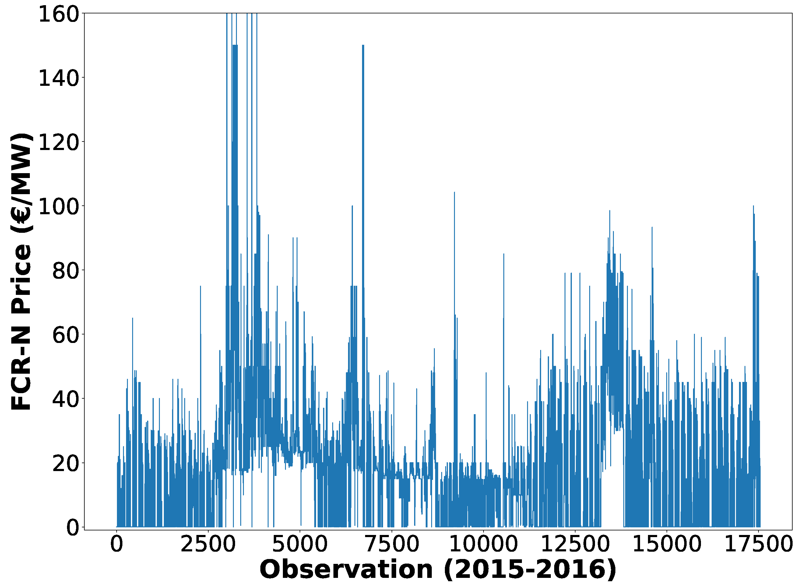
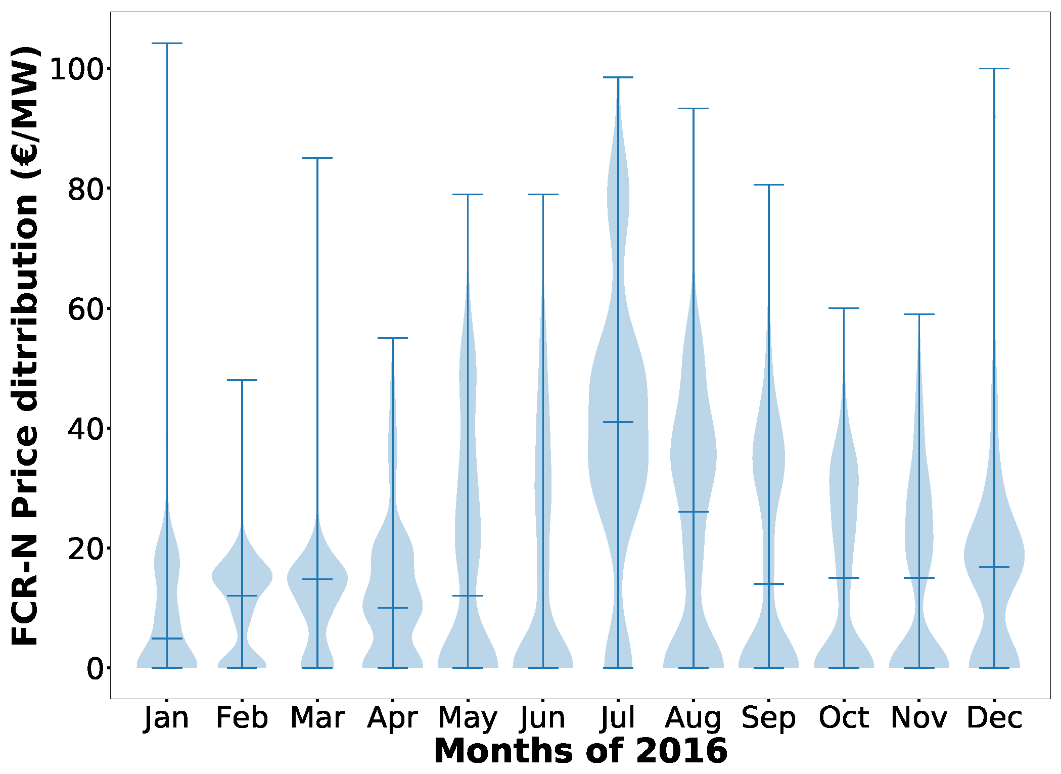
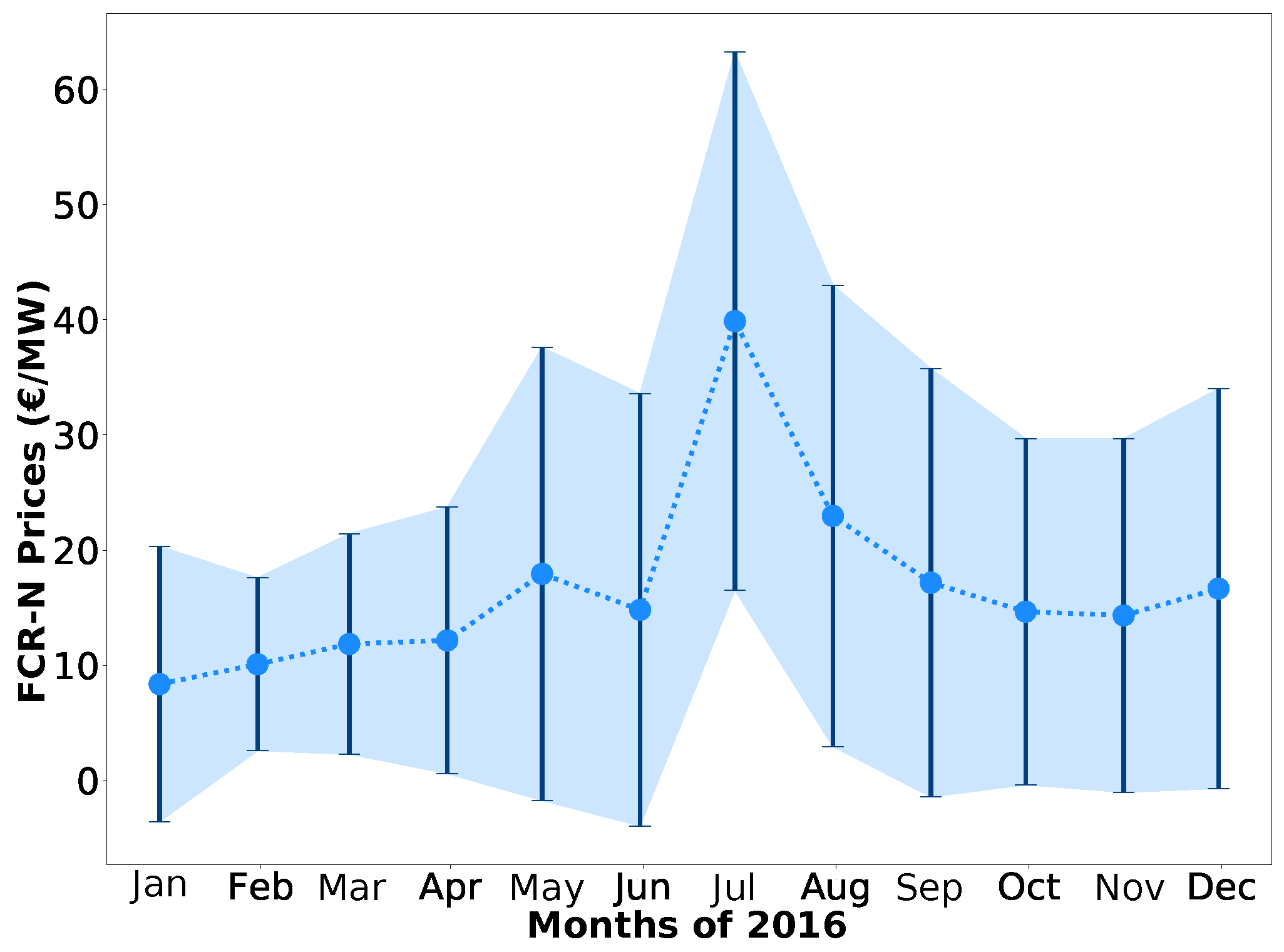
The FCR-N prices have been analyzed for the two years of data that were collected. Figure 1 shows the 17,544 observations of the FCR-N prices; the maximum price on the vertical axis was limited to 160 €/MW for clarity reasons, due to the small number of occurrences above this threshold. Figure 2 presents the violin plot [62] of the FCR-N prices for each month of 2016, which is the year targeted for the predictions in our empirical work. The figure shows the median and the distribution of the FCR-N price data. Moreover, Figure 3 displays the mean and the variance of the FCR-N prices for each month of 2016. Both Figure 2 and Figure 3 demonstrate that the FCR-N price data have a non-stationary distribution, where the data distribution, the monthly mean and variance changed considerably between consecutive months.
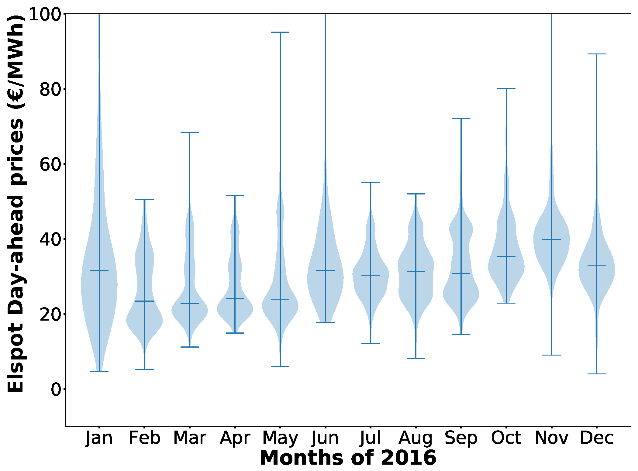
The statistics of the FCR-N prices are presented in Table 3. The skewness value of the data was large, demonstrating how the time series had a non-symmetric distribution. Furthermore, the kurtosis value shows that the data distribution was a leptokurtic distribution [54], characterized by heavy tails and sharp peaks around the mean. The large value of the Jarque–Bera test was a further indication that the FCR-N price data were far from being normally distributed. Moreover, comparing the distribution of the FCR-N prices (Figure 2) with the distribution of the Elspot market prices presented in Figure 4, it can be observed how the FCR-N prices behaved differently, with the data less distributed around the median and more towards the minimum and maximum value. A further difference with spot market prices was that the FCR-N prices were zero for around 30% of the time (Figure 2). Thus, any insights gained from predicting spot market prices could not be assumed to apply to this market.
Furthermore, several studies on spot market price prediction employ seasonal adjustment methods to remove the spot market seasonal component [54,63,64]. In fact, spot market prices present a strong seasonal behavior [43,63]. On the other hand, the FCR-N market presented a significantly weaker seasonality, with price patterns that can change considerably in a short period of time, as also shown by Figure 2 and Figure 3. Therefore, in contrast to the spot market prices, seasonal adjustment methods could not be employed in the methodology for the prediction of the FCR-N market prices.
3.3. Autocorrelation and Variable Lag
The autocorrelation of the FCR-N prices has been investigated for the data of 2016. Figure 5 shows the average autocorrelation of the FCR-N prices. It can be observed that the FCR-N prices presented a daily correlation (24-h lag), as well as a subordinate weekly correlation (168-h lag). Due to the daily correlation, a lag of 24 h was added to the variables for which no predictions were accessible for future times. Thus, the lag was added to all the variables except those belonging to the weather and calendar categories.
4. Methodology
The methodology that aimed at predicting the FCR-N prices was decomposed into five steps. In Section 4.1, a formulation of the prediction model is made, including the formulation for the employed ANN. A normalization preprocessing step of the input data is described in Section 4.2. Then, the employed validation method for the ANN prediction model is presented in Section 4.3, followed by the introduction of the performance measures utilized to evaluate the prediction performance of the ANN model (Section 4.4). In addition, the ANN model is empirically configured through the tuning of its hyper-parameters in Section 4.5.
4.1. Prediction Model Formulation
The primary objective of the study is to provide a solution for the prediction of the 24 distinct prices for each hour of the day-ahead FCR-N market prices. This means that the prediction horizon for our solution consisted of 24 distinct prices to be predicted. Thus, from the various machine learning strategies for time series forecasting [65], the Multi-Input Multi-Output (MIMO) strategy was selected [66]. The reason for using the MIMO strategy was that MIMO would return a vectorial forecast of the 24 h by modeling the time series in a multiple-input multiple-output regression model Therefore, through the MIMO strategy, it was possible to define a prediction model, which given as input n features, denoted by the matrix X, learned a function that generated as the output the prediction of the following time steps, denoted by the vector .
Usually, in machine learning, the input matrix X has the variables in rows and the training samples in columns. Similarly, each element of the vector is the prediction for one training sample. However, with the MIMO strategy with outputs, each training sample is a matrix X, and the prediction for each training sample is a vector with elements. Thus, the training sample X must have values for each variable. For one training sample at time t, the input matrix X and the output prediction vector are defined as:
where t represents the time in hours, while represents the variable 1 at time t and refers to the total number of elements in the matrix X.
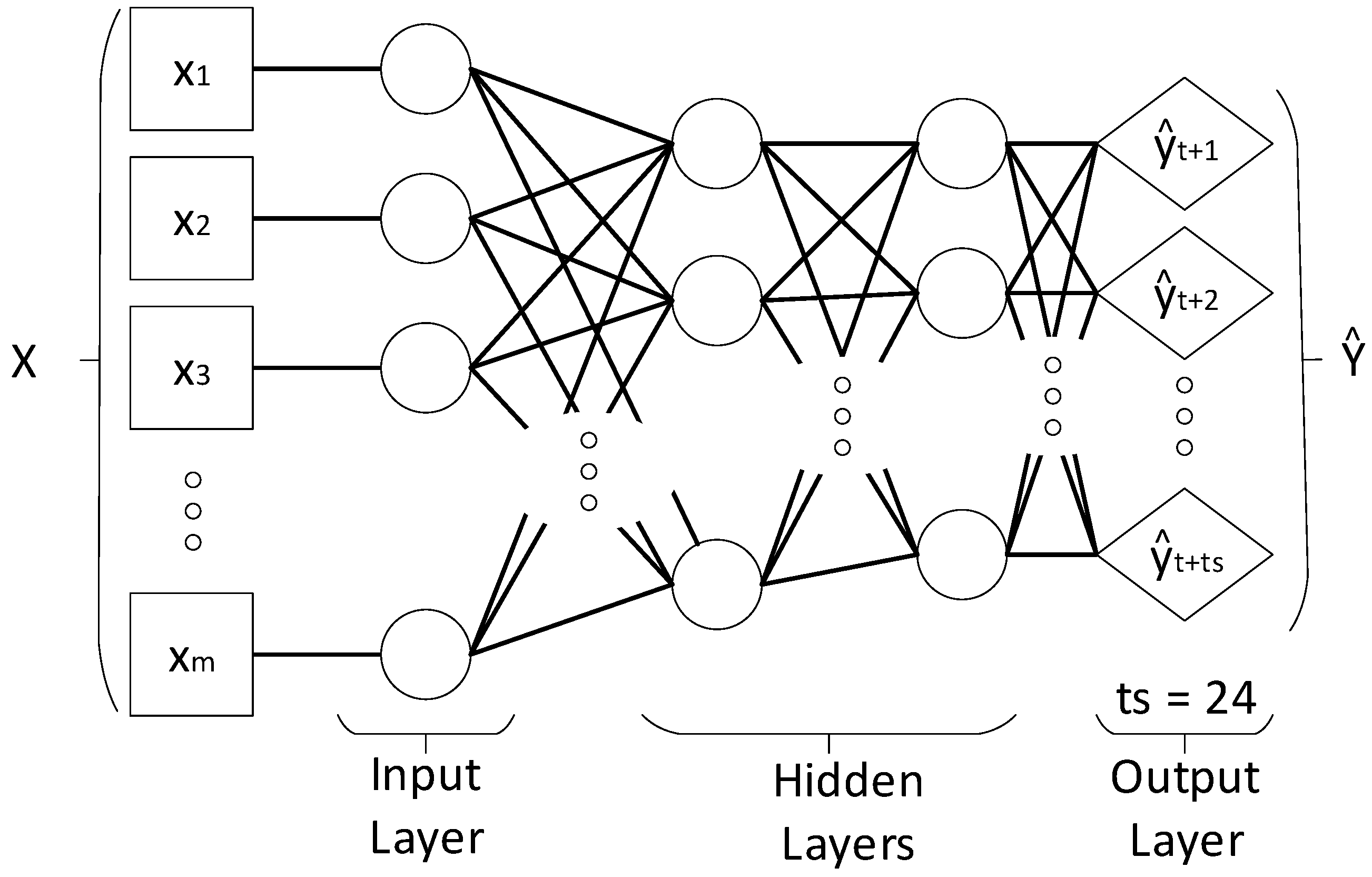
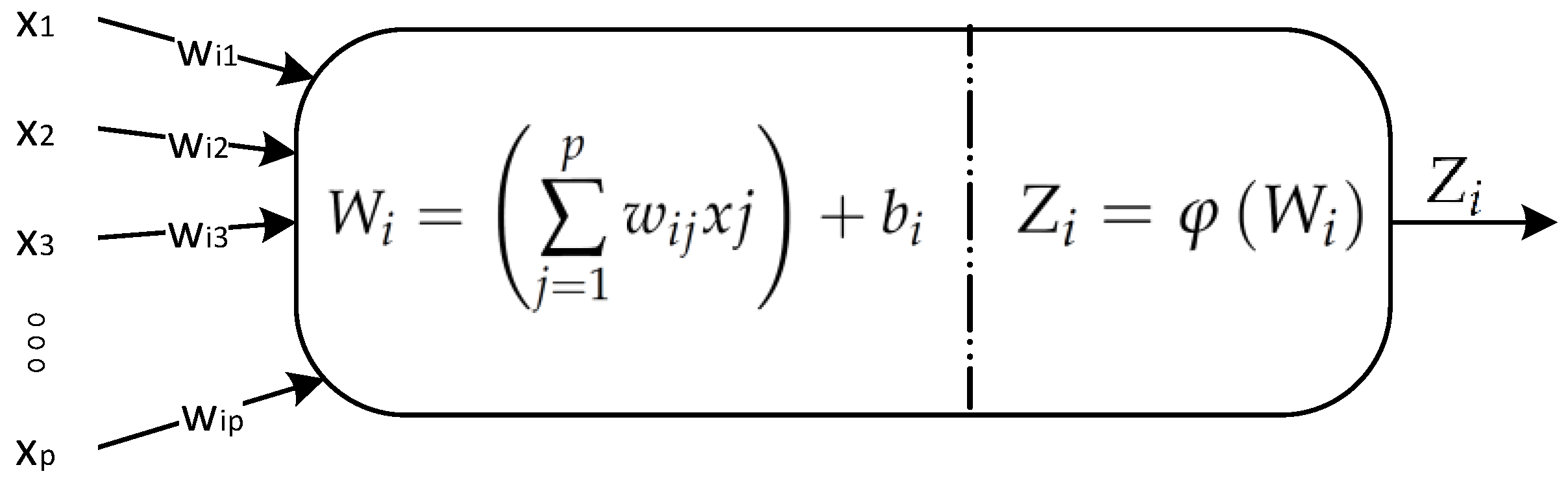
The model employed for the prediction of the FCR-N consisted of an ANN. The ANN technique is a computing system that mimics the function of the human brain and nerves, organized in such a way that the structure simulates a network. As shown in Figure 6, ANN can be composed by a certain amount of layers, which can be divided into three main categories: the input layer, the hidden layers and the output layer. The input layer consists of input nodes where the X matrix will be represented. The hidden layers consist of any layer in between the input and the output layer, while the output layer consists of the output variable to be predicted, i.e., . The key elements of an ANN are the neurons, which are depicted in Figure 7. Each neuron receives as input the output values () from each neuron of the previous layer with their respective weights and calculates a linear function as follows:
where p is the number of neurons of the previous layer and consists of a bias term. Then, in order to introduce nonlinearity into the ANN, thus allowing the ANN to better learn , each neuron applies a non-linear function to , also called the activation function , as follows:
4.2. Data Preprocessing
Each variable in the input matrix X needs to be normalized, in order to be standardized to the same range of values. In this study, a normalization method was chosen in order to rescale the features as a standard normal distribution [67]. The normalization method utilized was the unit variance [67]. Thus, the employed unit variance method distributed the variables in the range [−1,1], and it is specified as follows:
where is the mean of the distribution and the standard deviation.
4.3. Model Validation
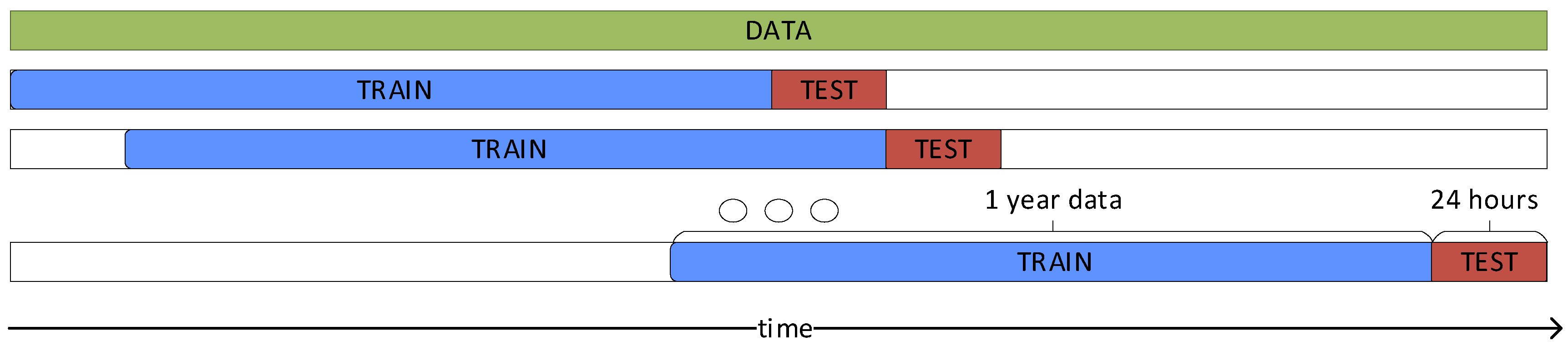
A forward validation method was employed to validate and select the best-performing ANN models [68]. Figure 8 shows the employed walk forward validation method, where an in-sample training dataset was utilized to train the prediction model, while an out-sample testing dataset was reserved for evaluating the prediction performance. The size of the sliding in-sample training dataset was determined by means of an experiment in Section 5.1.
Moreover, since the aim of this study is to predict the day-ahead price, the size of the testing dataset was set to 24 h of out-sample data. Finally, in the following Section 4.5, several datasets are formed and utilized to evaluate and select the best-performing prediction model. In time series prediction, contiguous subsets of data (in time) are segmented into two fractions (Figure 8) [69]. The first fraction is used for training the model and precedes the second fraction in the order of time, while the second fraction is used for testing. Thus, the performance is then evaluated by averaging the testing error over the several datasets generated with the walk forward validation method.
4.4. Prediction Performance Evaluation
Since the design of a neural network consists of an empirical process, where several models are tested and handcrafted, we need to define performance measures to evaluate which is the best-performing ANN model. In this study, of the several measures of prediction accuracy presented in the literature [43,70], in order to evaluate the prediction performance, we utilized the Mean Squared Error (MSE). The MSE is defined as follows:
where is the price data obtained from Fingrid, while is the predicted price. The decision to employ the MSE is mainly related to one key feature of the FCR-N prices, which present several instances of zero-values (Table 3). In fact, due to the large amount of zero-values in the FCR-N price data, several state of the art performance measures would produce a division by zero or an undefined division of zero by zero [70].
4.5. Empirical Configuration of an Artificial Neural Network
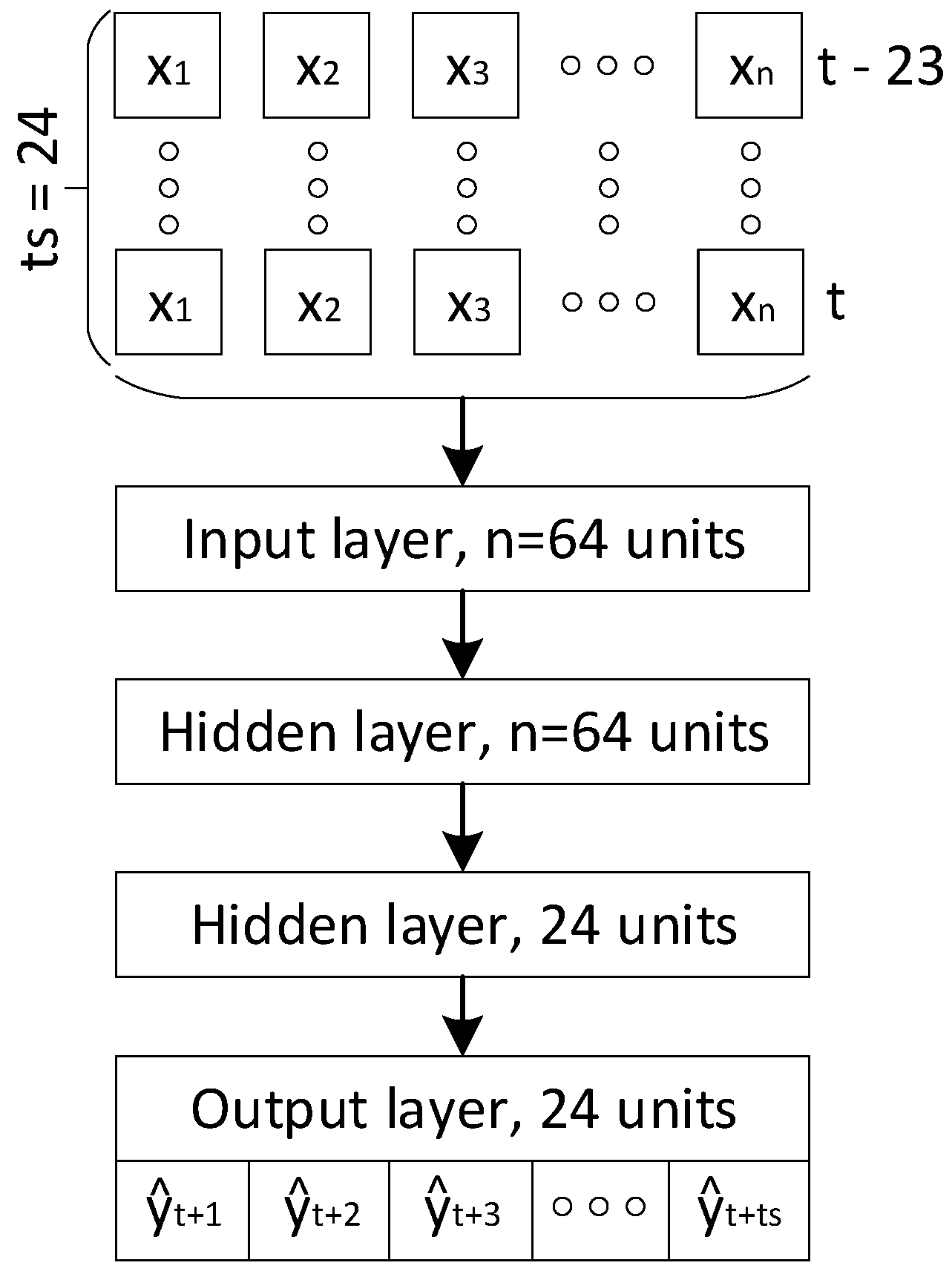
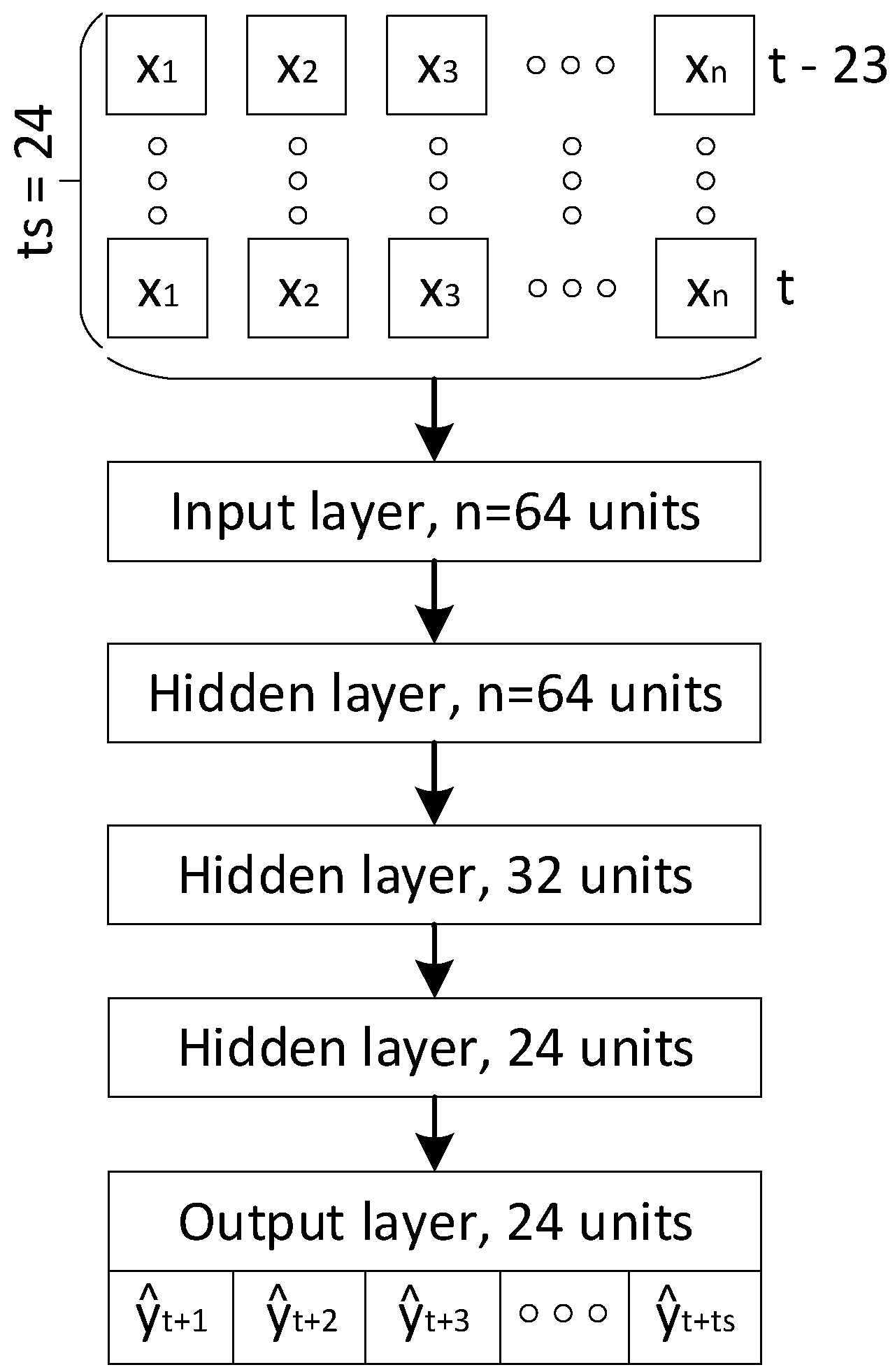
One of the first design decisions is the selection of the best-performing ANN architecture, which includes the identification of the activation functions, the number of hidden layers and the number of neurons for each layer. Currently, the selection of ANN architectures is executed by means of an empirical process [71], in which various architectures are tested, handcrafted and adjusted. General guidelines for designing an ANN architecture are well known among practitioners, as described in [72]. Following those guidelines, several architectures have been tested for the prediction of the FCR prices. Among those, in this study, we show the results of the two best-performing architectures, with the final aim of selecting the one that provides the best prediction performance. The two architectures compared in this study are presented in Figure 9 and Figure 10. The difference between the two architectures is that the architecture in Figure 9 is composed of 2 hidden layers, respectively containing and 24 neurons each. The architecture in Figure 10 has 3 hidden layers, respectively with , and 24 neurons each. In the following, the architecture of Figure 9 will be referred as the 3-layer architecture, due the fact that the depth of the architecture is , while the architecture in Figure 10 will be called the 4-layer architecture, since .
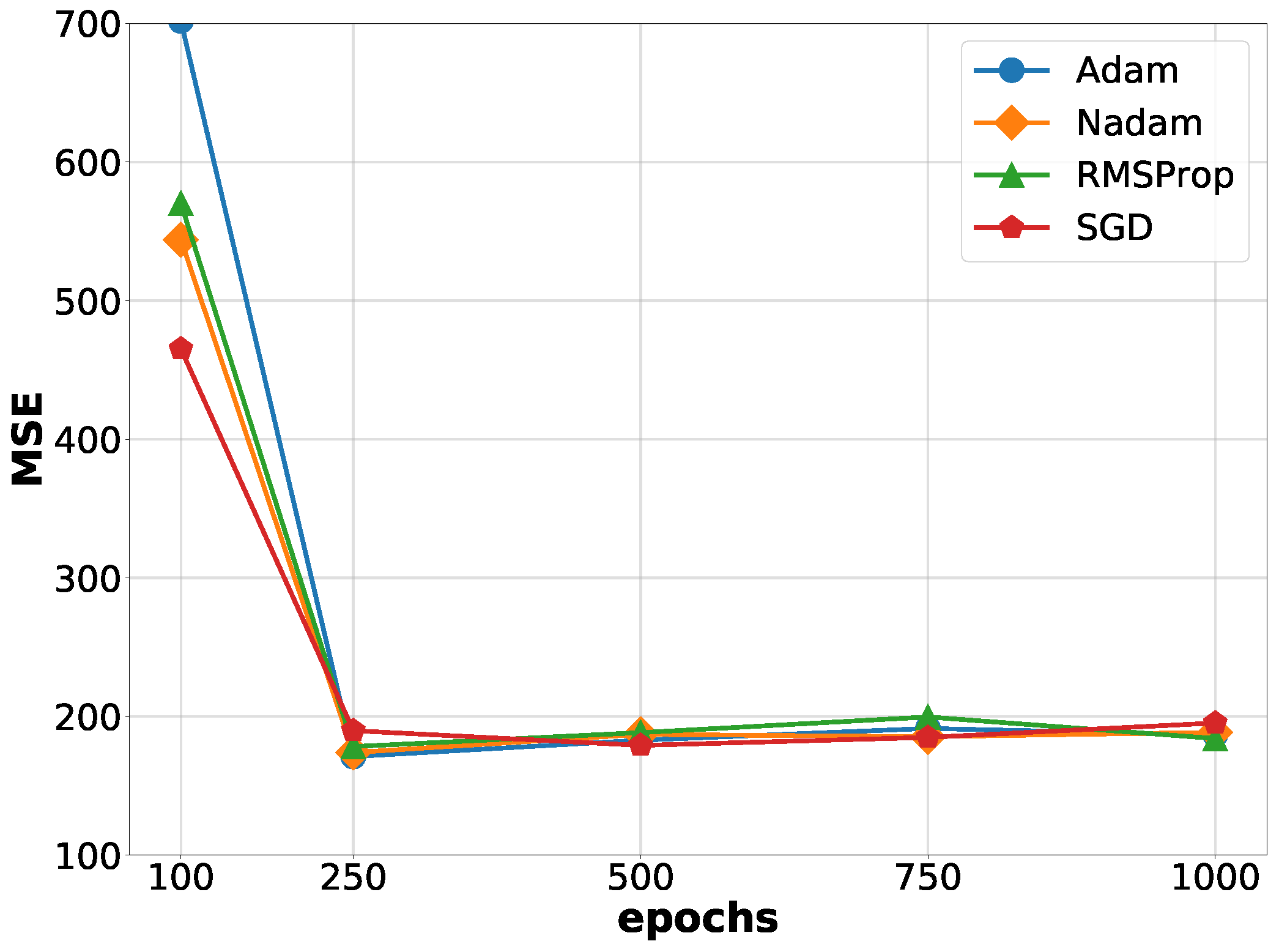
In order to compare the performance of the two ANN architectures, namely the 3-layer and the 4-layer, a set of gradient descent optimization algorithms has been employed. The set included the Stochastic Gradient Descent (SGD) [73], RMSProp [74], Adam [75] and Nadam [76]. The performance of the two architectures for the different gradient descent optimization algorithms are presented in Figure 11 for the 3-layer architecture and Figure 12 for the 4-layer. The two figures show how the 3-layer architecture had better performance than the 4-layer, while the difference in performance for the four gradient descent algorithms was less significant. The best performance was obtained by training the 3-layer architecture with 750 epochs. Thus, in the following, the 3-layer architecture was chosen for the FCR-N price predictions, where the Adam algorithm was utilized to optimize the gradient with 750 epochs, due to the fact that Adam provided the best MSE performance among the examined gradient descent algorithms.
One of the primary tasks when designing an ANN architecture is the identification of the best-performing activation functions. This identification is executed through an empirical process. Figure 13 compares the performance of the 3-layer architecture using different activation functions () for the hidden layers [77], namely tanh, softmax, ReLU and sigmoid. For this experiment, the ReLU function was used for the output layer, due the fact that the ReLU is defined as and the FCR-N prices are non-negative numbers. The box plot in Figure 13 shows the MSE prediction performance for a sample of thirty days uniformly distributed in the year 2016. This result shows that the best activation function for the hidden layers in terms of MSE performance is the sigmoid function. Thus, in the following, will be used as the activation function for the hidden layers, while for the output layer, will be used as the activation function.
In order to prevent the ANN model from overfitting, the dropout regularization was utilized for the FCR-N price predictions [78]. The dropout is a regularization technique that temporarily drops neurons from the ANN model during the training phase in a random order based on a probability p. For the selected 3-layer ANN model, a validation set of sixty days uniformly distributed in the year 2016 was utilized to identify the best dropout probability value p (expressed as a percentage %) for the FCR-N price predictions. The results of the experiment are presented in Figure 14, which shows the average MSE performance for each of the tested dropout probability values p. The results indicated that the best p-values were in the range of %, with being the best-performing value. Thus, a dropout probability value of was chosen for the 3-layer ANN model.
5. Empirical Results and Discussion
The selected ANN model for the experiments consisted of a three-layer model, as in Figure 9, where the gradient optimizer utilized was Adam with 750 epochs. Moreover, for the hidden layers, the selected activation function was the sigmoid, while for the output layer, the ReLU function was selected. Finally, a dropout value of 40% was utilized in order to prevent the ANN model from overfitting. In the following section, at first, the size of the training window for the ANN model is identified through an experiment (Section 5.1), then the prediction performance of the ANN model is extensively analyzed in Section 5.2. Section 5.3 completes the empirical experiments by comparing the prediction performance of the ANN model to two state of the art models.
5.1. Determining the Training Window Size
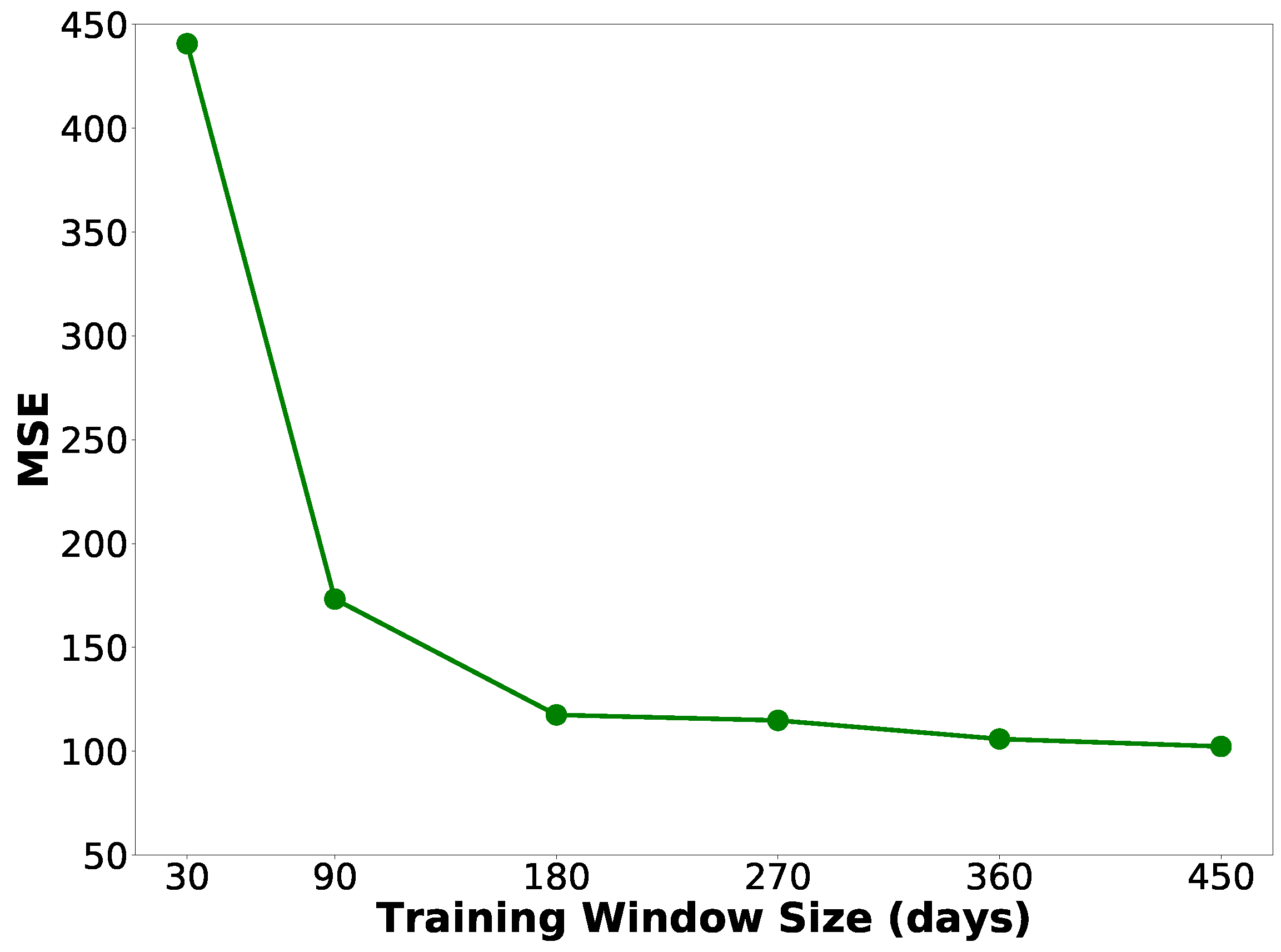
Since the FCR-N market is subject to rapid changes [57], it is necessary to establish a suitable window size to train the model. Therefore, an experiment was executed in order to define the size of the training window for the ANN model. Figure 15 shows the MSE for the 3-layer model for a sample of thirty days uniformly distributed, where it can be noted that the size of the training window tended to start stabilizing the prediction performance after 180 days on. Thus, since no fundamental improvements or degradations of the performance were registered with training window sizes larger than 360 day, the training window size chosen for the following experiments was 360 days, which is a good trade-off from being too small, thus starting to degrade the prediction performance, and from being too large, thus slowing the training of the ANN model. Moreover, further enlarging the training dataset could add noise to the prediction model, thus worsening the prediction performance. Hence, to summarize, in the following, the training window size is 360 days of data, while the testing window size corresponds to the 24 h ahead unless otherwise stated.
5.2. Prediction Performance Analysis
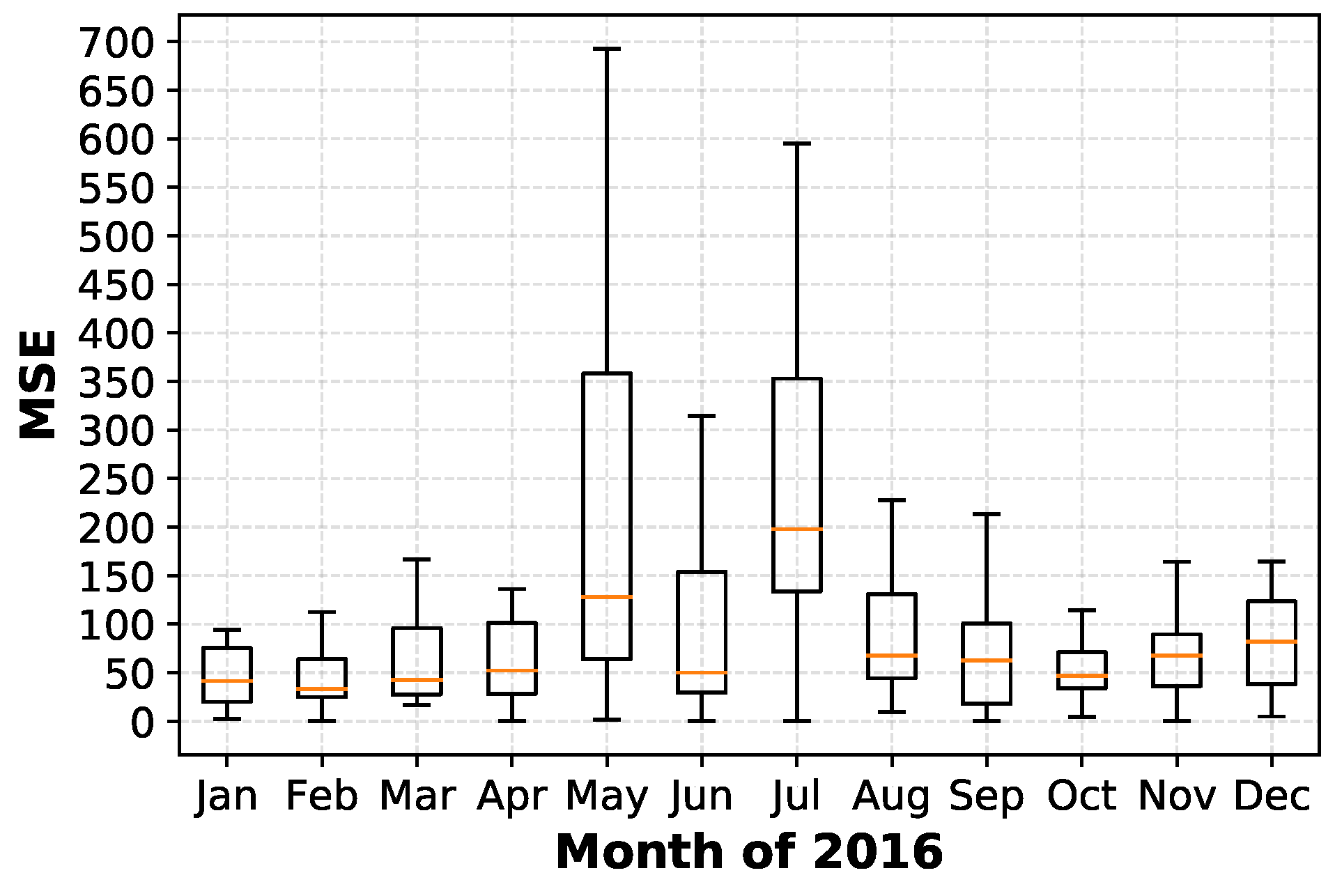
The prediction performance of the FCR-N prices was analyzed for the entirety of 2016 using the ANN model. For each day of 2016, one ANN model was trained for predicting the day-ahead FCR-N prices. Therefore, the first experiment aimed at analyzing the prediction performance for each month of the year 2016. As shown in Figure 2 and Figure 3, the FCR-N market prices have a fast-changing behavior even between consecutive months.Thus, this fast-changing behavior was also expected to affect the prediction performance. The prediction performance for each month of 2016 is presented in Figure 16 in the form of a box plot, where the median value is noted with a line within the boxes. As can be observed, the worse performance in the predictions was during the months of May and July. This performance result reflects the analysis presented in Section 3.2. In addition, the months of May and July presented a distribution of the price data, which differed considerably from their respective previous months (Figure 2), thus preventing the ANN model from learning the fast changes of the market efficiently.
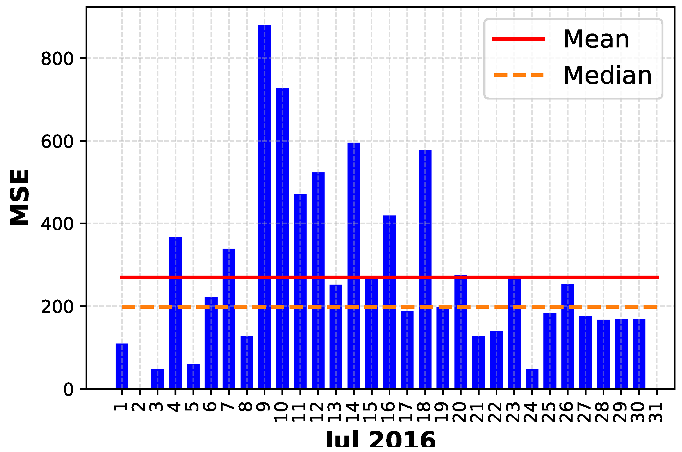
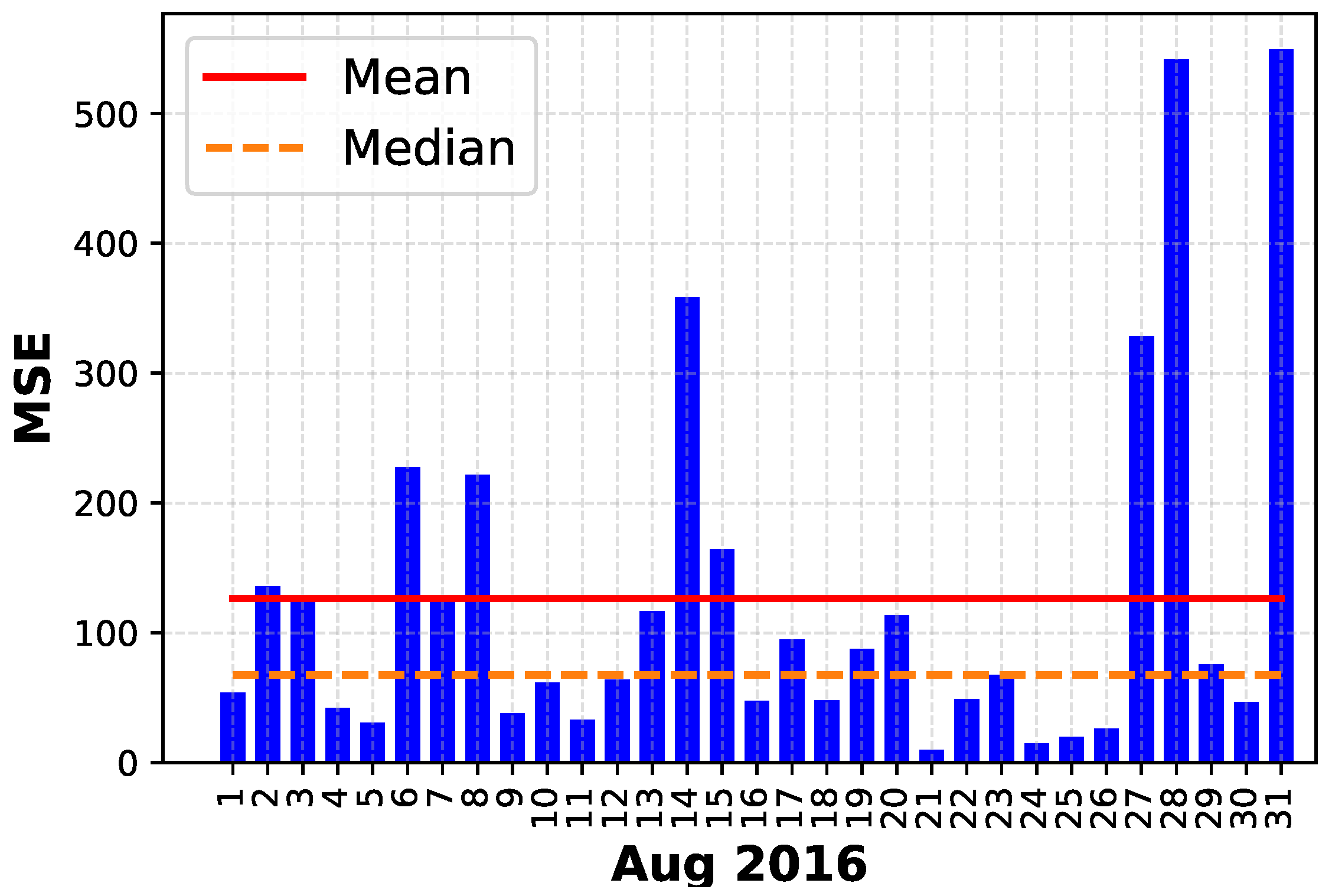
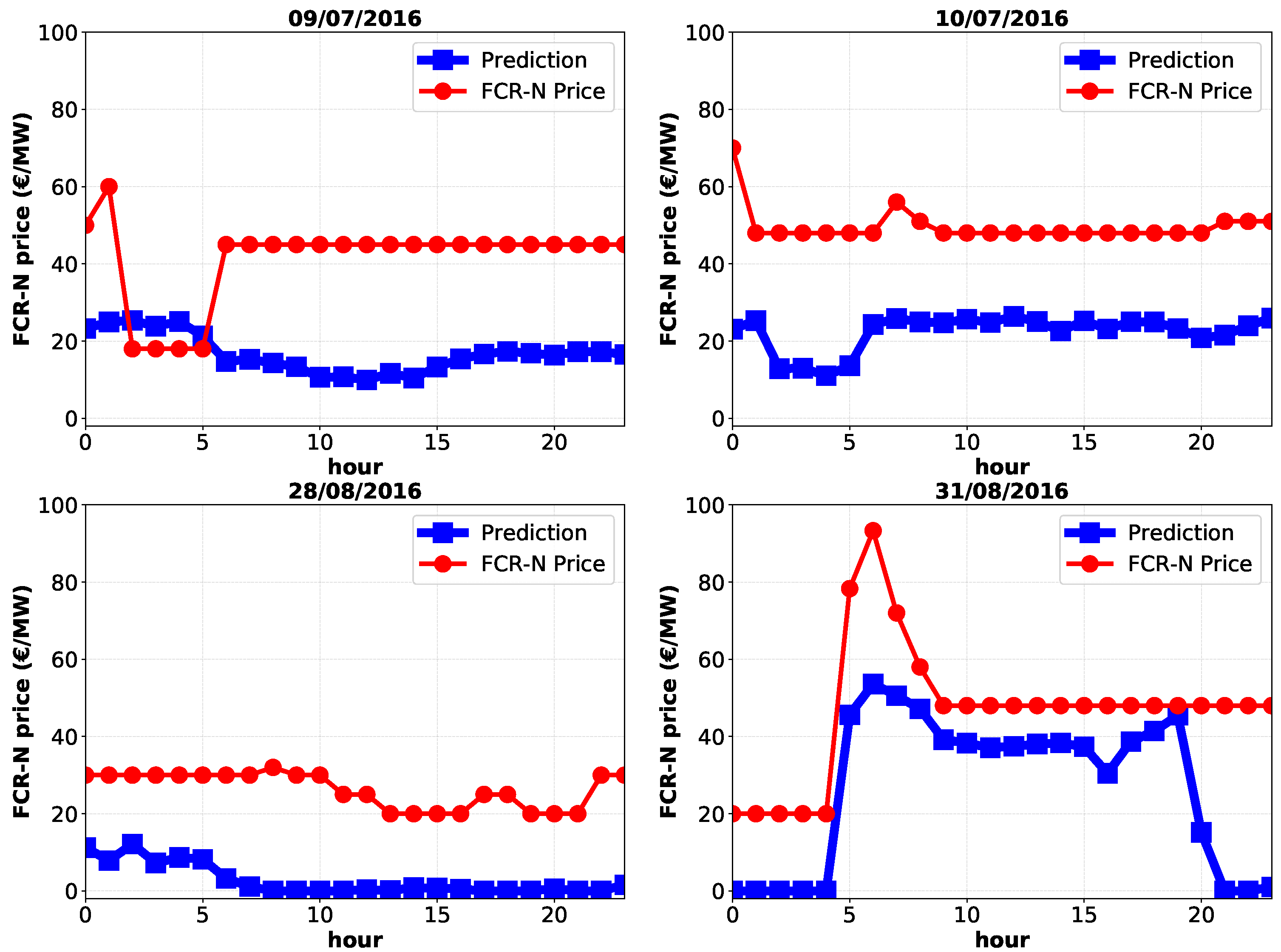
However, it can be noted that the median values in Figure 16 stand on the lower part of the respective boxes, demonstrating how the prediction performance was affected by a small number of outlier days. In fact, this can be observed by looking at the prediction performance more in detail. As examples, we analyzed the performance for the months of July and August, respectively the month with the higher variance and the next in the order of time. Thus, the prediction performance for each day of July and August is presented in Figure 17 and Figure 18, respectively, where the monthly mean and median of the MSE of each day are also represented. The figures show how the difference between the mean and the median of the performance was due to a small set of outlier days. The main four outlier days of July and August are presented in Figure 19. All the outlier days present very unusual price patterns, which were not registered in the past observations, making them exceptionally difficult to predict.
On the other hand, Figure 20 shows the prediction of the FCR-N prices for four days in the time span of two weeks between July and August 2016. As can be noted, the pattern of the FCR-N prices could vary quite rapidly in a short time period, making the FCR-N price prediction more challenging than the spot prices, which presented an evident seasonality between contiguous days. Moreover, the first row in Figure 21 presents two days with an outlier behavior (i.e., price patterns specific to the analyzed period of time and not commonly observed in other periods), which were adequately predicted by the ANN model. In the second row of Figure 21 is shown two price patterns with their respective predictions, which recurred regularly along the entire period of time analyzed (i.e., 2015–2106), where the ANN model succeeded to provide accurate predictions.
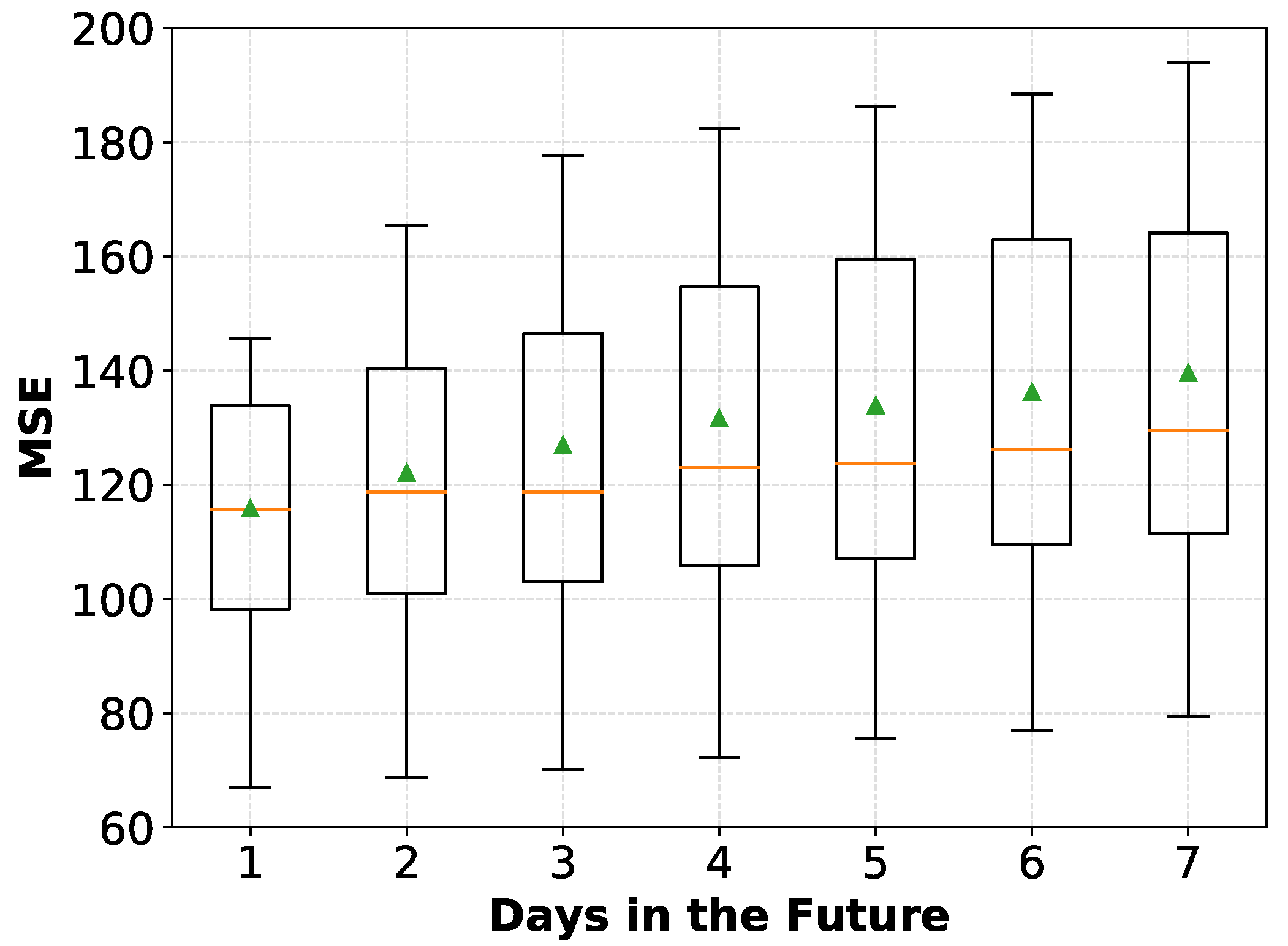
Part of the methodology involves the decision on how often the computationally-intensive retraining of the ANN needs to be performed. Thus, the second experiment aimed at analyzing how the performance of the ANN model degraded when the ANN model was utilized for predicting several days in the future without a retraining of the model. Figure 21 presents the prediction performance (in terms of MSE) of the ANN model up to seven days in the future for the year 2016, where the median of the daily performance is represented with a line, while the daily mean performance is represented as a triangle. The prediction performance degraded linearly with respect to the number of days in the future to be predicted, going from an MSE of 115.8 for the first day to 139.6 for the seventh day after training the ANN model. At the same time, the distance between the median and the mean, as well as the variance of the prediction performance increased, indicating that a short retraining period of the ANN model was desirable to reduce the prediction errors on outlier price patterns.
5.3. Comparison with the State of the Art
The last experiment aimed at comparing the prediction performance of the ANN model with two state of the art methods. The two selected methods were SVR and ARIMA, respectively, which were employed as benchmarks of the state of the art for predicting the FCR-N prices. Therefore, an SVR model was trained with the same training data as for the ANN model, i.e., with the X matrix as the input. While for the ARIMA model, one-year FCR-N price data prior to the day to be predicted were used as the training data, where the ARIMA parameters (i.e., respectively autoregressive, differencing and moving average parameters) are . Similarly to the ANN model, the test window size was for the 24 h of the day-ahead for both selected methods (i.e., SVR and ARIMA).
Figure 22 compares the FCR-N price prediction performance of the ANN model with the two selected benchmark models: SVR and . The results revealed how the ANN model outperformed the SVR, as well as the ARIMA. The results showed how during the first four months of the year, when the prices were distributed around the median and had a low variance, the three models had similar performance, even if the ANN model always outperformed the other two models. However, once the prices experienced an increase in the variance and a dispersion from the median value (i.e., between May and August), the ARIMA failed to adapt to the fast changes of the FCR-N prices, while the ANN model provided predictions with a superior accuracy even compared to the SVR model. Further, the ARIMA predictions for the last few months of 2016 (i.e., September–December), where the FCR-N prices have a similar behavior, were largely affected by the previous period (i.e., May–August), showing how the ARIMA failed to adapt to the new changes of the prices. On the contrary, the ANN model was capable of adapting also in the third period of the experimented year and significantly outperformed the ARIMA benchmark, without being affected by the noise of the prices from the preceding period (i.e., May–August). In addition, for the same period, the ANN model performed better than the SVR model, which resulted in being more robust to the noise introduced by the previous prices than ARIMA. Thus, ANN was shown to outperform the ARIMA benchmark model largely, being more capable of adapting to new price patterns, while maintaining memory of the patterns occurring regularly and being more robust to the fast changes occurring in the FCR-N market prices. Moreover, the ANN also outperformed the prediction performance of the SVR model.
6. Conclusions
The objective of this study was to predict the day-ahead prices for ancillary markets, with the FCR-N market as a case study. The study outlined the problem analysis and methodology used to predict the FCR-N market prices. The problem analysis consisted of identifying the relevant data sources available for the predictions and then continued by analyzing the FCR-N market prices and their substantial differences from the spot market prices. Moreover, the methodology outlined the selected MIMO strategy for time series forecasting. Then, the methodology defined the data preprocessing and utilized the model validation method and the performance evaluation coefficient. Finally, the methodology introduced the main design decisions that were made for the configuration of the ANN model, which consisted of tuning several hyper-parameters through an empirical process.
In Section 5, the performance of the developed ANN model for the prediction of FCR-N market prices was analyzed. At first, the size of the training window size was determined through an experiment. Then, the predictions for the entire year 2016 were analyzed in detail, demonstrating that the performances were affected by a small set of outlier days. Moreover, a third experiment proved how a frequent retraining of the ANN model can mitigate the effect of the outlier days on the prediction performance. Finally, the last experiment aimed at showing how the developed ANN model outperformed two benchmark state of the art models, namely the SVR and ARIMA models, in the prediction of the FCR-N market prices.
Author Contributions
C.G. conceived, designed and performed the experiments; C.G. analyzed the data; C.G. and S.S. wrote the paper; R.I., V.V. and S.S. supervised the work and helped to improve the quality of the manuscript.
Funding
The research has been funded by the project “Harnessing the consumer for a flexible energy system architecture” (285029) of the Academy of Finland and by the Finnish Society of Automation.
Acknowledgments
The calculations presented above were performed using computer resources within the Aalto University School of Science “Science-IT” project and the GPU servers provided by the Ichise laboratory at the National Institute of Informatics.
Conflicts of Interest
The authors declare no conflict of interest.
Abbreviations
| aFRR | Automatic Frequency Restoration Reserve |
| ANN | Artificial Neural Network |
| ARIMA | AutoRegressive Integrated Moving Average |
| DER | Distributed Energy Resources |
| DR | Demand Response |
| EV | Electric Vehicle |
| FCR | Frequency Containment Reserve |
| FCR-D | Frequency Containment Reserve for Disturbance |
| FCR-N | Frequency Containment Reserve for Normal operation |
| MIMO | Multi-Input Multi-Output |
| MSE | Mean Squared Error |
| RNN | Recurrent Neural Network |
| SGD | Stochastic Gradient Descent |
| SVR | Support Vector Regression |
| V2B | Vehicle-to-Building |
| V2H | Vehicle-to-Home |
References
- Gkatzikis, L.; Koutsopoulos, I.; Salonidis, T. The role of aggregators in smart grid demand response markets. IEEE J. Sel. Areas Commun. 2013, 31, 1247–1257. [Google Scholar] [CrossRef]
- Wang, Z.; Wang, L. Adaptive negotiation agent for facilitating bi-directional energy trading between smart building and utility grid. IEEE Trans. Smart Grid 2013, 4, 702–710. [Google Scholar] [CrossRef]
- He, Y.; Venkatesh, B.; Guan, L. Optimal scheduling for charging and discharging of electric vehicles. IEEE Trans. Smart Grid 2012, 3, 1095–1105. [Google Scholar] [CrossRef]
- Xie, D.; Chu, H.; Gu, C.; Li, F.; Zhang, Y. A novel dispatching control strategy for EVs intelligent integrated stations. IEEE Trans. Smart Grid 2017, 8, 802–811. [Google Scholar] [CrossRef]
- Berthold, F.; Ravey, A.; Blunier, B.; Bouquain, D.; Williamson, S.; Miraoui, A. Design and development of a smart control strategy for plug-in hybrid vehicles including vehicle-to-home functionality. IEEE Trans. Trans. Electrif. 2015, 1, 168–177. [Google Scholar] [CrossRef]
- Pang, C.; Dutta, P.; Kezunovic, M. BEVs/PHEVs as dispersed energy storage for V2B uses in the smart grid. IEEE Trans. Smart Grid 2012, 3, 473–482. [Google Scholar] [CrossRef]
- Jia, Q.S.; Shen, J.X.; Xu, Z.B.; Guan, X.H. Simulation-based policy improvement for energy management in commercial office buildings. IEEE Trans. Smart Grid 2012, 3, 2211–2223. [Google Scholar] [CrossRef]
- Venayagamoorthy, G.K.; Sharma, R.K.; Gautam, P.K.; Ahmadi, A. Dynamic energy management system for a smart microgrid. IEEE Trans. Neural Netw. Learn. Syst. 2016, 27, 1643–1656. [Google Scholar] [CrossRef] [PubMed]
- De Angelis, F.; Boaro, M.; Fuselli, D.; Squartini, S.; Piazza, F.; Wei, Q. Optimal home energy management under dynamic electrical and thermal constraints. IEEE Trans. Ind. Inform. 2013, 9, 1518–1527. [Google Scholar] [CrossRef]
- Wu, D.; Aliprantis, D.C.; Ying, L. Load scheduling and dispatch for aggregators of plug-in electric vehicles. IEEE Trans. Smart Grid 2012, 3, 368–376. [Google Scholar] [CrossRef]
- Zhang, T.; Chen, W.; Han, Z.; Cao, Z. Charging scheduling of electric vehicles with local renewable energy under uncertain electric vehicle arrival and grid power price. IEEE Trans. Veh. Technol. 2014, 63, 2600–2612. [Google Scholar] [CrossRef]
- Bahrami, S.; Amini, M.H.; Shafie-khah, M.; Catalao, J.P. A decentralized electricity market scheme enabling demand response deployment. IEEE Trans. Power Syst. 2018, 33, 4218–4227. [Google Scholar] [CrossRef]
- Callaway, D.S.; Hiskens, I.A. Achieving controllability of electric loads. Proc. IEEE 2011, 99, 184–199. [Google Scholar] [CrossRef]
- Zhang, X.; Hug, G.; Kolter, J.Z.; Harjunkoski, I. Demand response of ancillary service from industrial loads coordinated with energy storage. IEEE Trans. Power Syst. 2018, 33, 951–961. [Google Scholar] [CrossRef]
- Wandhare, R.G.; Agarwal, V. Novel stability enhancing control strategy for centralized PV-grid systems for smart grid applications. IEEE Trans. Smart Grid 2014, 5, 1389–1396. [Google Scholar] [CrossRef]
- Liu, M.; Shi, Y.; Liu, X. Distributed MPC of aggregated heterogeneous thermostatically controlled loads in smart grid. IEEE Trans. Ind. Electron. 2016, 63, 1120–1129. [Google Scholar] [CrossRef]
- Jin, C.; Lu, N.; Lu, S.; Makarov, Y.V.; Dougal, R.A. A coordinating algorithm for dispatching regulation services between slow and fast power regulating resources. IEEE Trans. Smart Grid 2014, 5, 1043–1050. [Google Scholar] [CrossRef]
- Lu, N.; Zhang, Y. Design considerations of a centralized load controller using thermostatically controlled appliances for continuous regulation reserves. IEEE Trans. Smart Grid 2013, 4, 914–921. [Google Scholar] [CrossRef]
- Galus, M.D.; Koch, S.; Andersson, G. Provision of load frequency control by PHEVs, controllable loads, and a cogeneration unit. IEEE Trans. Ind. Electron. 2011, 58, 4568–4582. [Google Scholar] [CrossRef]
- Ota, Y.; Taniguchi, H.; Nakajima, T.; Liyanage, K.M.; Baba, J.; Yokoyama, A. Autonomous distributed V2G (vehicle-to-grid) satisfying scheduled charging. IEEE Trans. Smart Grid 2012, 3, 559–564. [Google Scholar] [CrossRef]
- Gu, Y.; Bakke, J.; Zhou, Z.; Osborn, D.; Guo, T.; Bo, R. A novel market simulation methodology on hydro storage. IEEE Trans. Smart Grid 2014, 5, 1119–1128. [Google Scholar] [CrossRef]
- Ilić, M.D.; Popli, N.; Joo, J.Y.; Hou, Y. A possible engineering and economic framework for implementing demand side participation in frequency regulation at value. In Proceedings of the 2011 IEEE Power and Energy Society General Meeting, Detroit, MI, USA, 24–28 July 2011; pp. 1–7. [Google Scholar]
- Fingrid. Rules and Fees for the Hourly Market of Frequency Controlled Reserves. 2018. Available online: https://goo.gl/Lx62YR (accessed on 21 July 2018).
- Wu, D.; Zeng, H.; Lu, C.; Boulet, B. Two-stage energy management for office buildings with workplace EV charging and renewable energy. IEEE Trans. Transp. Electrif. 2017, 3, 225–237. [Google Scholar] [CrossRef]
- Wang, P.; Zareipour, H.; Rosehart, W.D. Descriptive models for reserve and regulation prices in competitive electricity markets. IEEE Trans. Smart Grid 2014, 5, 471–479. [Google Scholar] [CrossRef]
- Vagropoulos, S.I.; Kyriazidis, D.K.; Bakirtzis, A.G. Real-time charging management framework for electric vehicle aggregators in a market environment. IEEE Trans. Smart Grid 2016, 7, 948–957. [Google Scholar] [CrossRef]
- Shafie-khah, M.; Catalão, J.P. A stochastic multi-layer agent-based model to study electricity market participants behavior. IEEE Trans. Power Syst. 2015, 30, 867–881. [Google Scholar] [CrossRef]
- Sánchez-Martín, P.; Lumbreras, S.; Alberdi-Alén, A. Stochastic programming applied to EV charging points for energy and reserve service markets. IEEE Trans. Power Syst. 2016, 31, 198–205. [Google Scholar] [CrossRef]
- Jin, C.; Tang, J.; Ghosh, P. Optimizing electric vehicle charging with energy storage in the electricity market. IEEE Trans. Smart Grid 2013, 4, 311–320. [Google Scholar] [CrossRef]
- Han, S.; Han, S.; Sezaki, K. Development of an optimal vehicle-to-grid aggregator for frequency regulation. IEEE Trans. Smart Grid 2010, 1, 65–72. [Google Scholar]
- Melo, D.R.; Trippe, A.; Gooi, H.B.; Massier, T. Robust electric vehicle aggregation for ancillary service provision considering battery aging. IEEE Trans. Smart Grid 2016, 9. [Google Scholar] [CrossRef]
- Ela, E.; Gevorgian, V.; Tuohy, A.; Kirby, B.; Milligan, M.; O’Malley, M. Market designs for the primary frequency response ancillary service—Part I: Motivation and design. IEEE Trans. Power Syst. 2014, 29, 421–431. [Google Scholar] [CrossRef]
- Ela, E.; Gevorgian, V.; Tuohy, A.; Kirby, B.; Milligan, M.; O’Malley, M. Market designs for the primary frequency response ancillary service—Part II: Case studies. IEEE Trans. Power Syst. 2014, 29, 432–440. [Google Scholar] [CrossRef]
- González, P.; Villar, J.; Díaz, C.A.; Campos, F.A. Joint energy and reserve markets: Current implementations and modeling trends. Electr. Power Syst. Res. 2014, 109, 101–111. [Google Scholar] [CrossRef]
- Raineri, R.; Rios, S.; Schiele, D. Technical and economic aspects of ancillary services markets in the electric power industry: An international comparison. Energy Policy 2006, 34, 1540–1555. [Google Scholar] [CrossRef]
- Fingrid. Frequency Containment Reserves. 2018. Available online: https://goo.gl/aY2PSE (accessed on 21 July 2018).
- ENTSO-E. Nordic Balancing Philosophy. 2016. Available online: https://goo.gl/Hn6o3D (accessed on 21 July 2018).
- Yang, J.; Zhao, J.; Luo, F.; Wen, F.; Dong, Z.Y. Decision-making for electricity retailers: A brief survey. IEEE Trans. Smart Grid 2017. [Google Scholar] [CrossRef]
- Croonenbroeck, C.; Hüttel, S. Quantifying the economic efficiency impact of inaccurate renewable energy price forecasts. Energy 2017, 134, 767–774. [Google Scholar] [CrossRef]
- Wang, P.; Zareipour, H.; Rosehart, W.D. Characteristics of the prices of operating reserves and regulation services in competitive electricity markets. Energy Policy 2011, 39, 3210–3221. [Google Scholar] [CrossRef]
- Fingrid. Market Places. 2017. Available online: https://goo.gl/QfddQ1 (accessed on 21 July 2018).
- Karthikeyan, S.P.; Raglend, I.J.; Kothari, D.P. A review on market power in deregulated electricity market. Int. J. Electr. Power Energy Syst. 2013, 48, 139–147. [Google Scholar] [CrossRef]
- Weron, R. Electricity price forecasting: A review of the state-of-the-art with a look into the future. Int. J. Forecast. 2014, 30, 1030–1081. [Google Scholar] [CrossRef]
- Domanski, P.D.; Gintrowski, M. Alternative approaches to the prediction of electricity prices. Int. J. Energy Sect. Manag. 2017, 11, 3–27. [Google Scholar] [CrossRef]
- Contreras, J.; Espinola, R.; Nogales, F.J.; Conejo, A.J. ARIMA models to predict next-day electricity prices. IEEE Trans. Power Syst. 2003, 18, 1014–1020. [Google Scholar] [CrossRef] [Green Version]
- Keles, D.; Scelle, J.; Paraschiv, F.; Fichtner, W. Extended forecast methods for day-ahead electricity spot prices applying artificial neural networks. Appl. Energy 2016, 162, 218–230. [Google Scholar] [CrossRef]
- Gao, G.; Lo, K.; Fan, F. Comparison of ARIMA and ANN models used in electricity price forecasting for power market. Energy Power Eng. 2017, 9, 120–126. [Google Scholar] [CrossRef]
- Drucker, H.; Burges, C.J.; Kaufman, L.; Smola, A.J.; Vapnik, V. Support vector regression machines. In Advances in Neural Information Processing Systems; Mit Press: Cambridge, MA, USA, 1997; pp. 155–161. [Google Scholar]
- Zhao, J.H.; Dong, Z.Y.; Xu, Z.; Wong, K.P. A statistical approach for interval forecasting of the electricity price. IEEE Trans. Power Syst. 2008, 23, 267–276. [Google Scholar] [CrossRef]
- Shayeghi, H.; Ghasemi, A.; Moradzadeh, M.; Nooshyar, M. Simultaneous day-ahead forecasting of electricity price and load in smart grids. Energy Convers. Manag. 2015, 95, 371–384. [Google Scholar] [CrossRef]
- Shiri, A.; Afshar, M.; Rahimi-Kian, A.; Maham, B. Electricity price forecasting using Support Vector Machines by considering oil and natural gas price impacts. In Proceedings of the 2015 IEEE International Conference on Smart Energy Grid Engineering (SEGE), Oshawa, ON, Canada, 17–19 August 2015; pp. 1–5. [Google Scholar]
- Giovanelli, C.; Liu, X.; Sierla, S.; Vyatkin, V.; Ichise, R. Towards an aggregator that exploits big data to bid on frequency containment reserve market. In Proceedings of the IECON 2017 43rd Annual Conference of the IEEE Industrial Electronics Society, Beijing, China, 29 October–1 November 2017; pp. 7514–7519. [Google Scholar]
- Panapakidis, I.P.; Dagoumas, A.S. Day-ahead electricity price forecasting via the application of artificial neural network based models. Appl. Energy 2016, 172, 132–151. [Google Scholar] [CrossRef]
- Saâdaoui, F. A seasonal feedforward neural network to forecast electricity prices. Neural Comput. Appl. 2017, 28, 835–847. [Google Scholar] [CrossRef]
- Sharma, V.; Srinivasan, D. A hybrid intelligent model based on recurrent neural networks and excitable dynamics for price prediction in deregulated electricity market. Eng. Appl. Artif. Intell. 2013, 26, 1562–1574. [Google Scholar] [CrossRef]
- Kaastra, I.; Boyd, M. Designing a neural network for forecasting financial and economic time series. Neurocomputing 1996, 10, 215–236. [Google Scholar] [CrossRef] [Green Version]
- Ahlstrom, M.; Ela, E.; Riesz, J.; O’Sullivan, J.; Hobbs, B.F.; O’Malley, M.; Milligan, M.; Sotkiewicz, P.; Caldwell, J. The Evolution of the Market: Designing a Market for High Levels of Variable Generation. IEEE Power Energy Mag. 2015, 13, 60–66. [Google Scholar] [CrossRef]
- Fingrid. Fingrid Open Data Service. 2017. Available online: https://data.fingrid.fi (accessed on 21 July 2018).
- Energia.fi. Finnish Electricity Consumption. 2017. Available online: https://energia.fi/EN (accessed on 21 July 2018).
- NordPool. Day-ahead Elspot prices. 2017. Available online: http://www.nordpoolspot.com/historical-market-data/ (accessed on 21 July 2018).
- Finnish Meteorological Institute. Finnish Meteorological Institute’s Open Data. Available online: https://en.ilmatieteenlaitos.fi/open-data (accessed on 21 July 2018).
- Hintze, J.L.; Nelson, R.D. Violin plots: A box plot-density trace synergism. Am. Stat. 1998, 52, 181–184. [Google Scholar]
- Marcjasz, G.; Uniejewski, B.; Weron, R. On the importance of the long-term seasonal component in day-ahead electricity price forecasting with NARX neural networks. Int. J. Forecast. 2018. [Google Scholar] [CrossRef]
- Zhou, Z.; Chan, W.K.V. Reducing electricity price forecasting error using seasonality and higher order crossing information. IEEE Trans. Power Syst. 2009, 24, 1126–1135. [Google Scholar] [CrossRef]
- Bontempi, G.; Ben Taieb, S.; Le Borgne, Y.A. Machine Learning Strategies for Time Series Forecasting; Springer: Berlin/Heidelberg, Germany, 2013; pp. 62–77. [Google Scholar]
- An, N.H.; Anh, D.T. Comparison of Strategies for Multi-step-Ahead Prediction of Time Series Using Neural Network. In Proceedings of the 2015 International Conference on Advanced Computing and Applications (ACOMP), Ho Chi Minh City, Vietnam, 23–25 November 2015; pp. 142–149. [Google Scholar]
- Aksoy, S.; Haralick, R.M. Feature normalization and likelihood-based similarity measures for image retrieval. Pattern Recognit. Lett. 2001, 22, 563–582. [Google Scholar] [CrossRef] [Green Version]
- Bergmeir, C.; Benítez, J.M. On the use of cross-validation for time series predictor evaluation. Inf. Sci. 2012, 191, 192–213. [Google Scholar] [CrossRef]
- Bergmeir, C.; Hyndman, R.J.; Koo, B. A note on the validity of cross-validation for evaluating autoregressive time series prediction. Comput. Stat. Data Anal. 2018, 120, 70–83. [Google Scholar] [CrossRef]
- Hyndman, R.J.; Koehler, A.B. Another look at measures of forecast accuracy. Int. J. Forecast. 2006, 22, 679–688. [Google Scholar] [CrossRef] [Green Version]
- Baker, B.; Gupta, O.; Naik, N.; Raskar, R. Designing neural network architectures using reinforcement learning. arXiv, 2016; arXiv:1611.02167. [Google Scholar]
- Heaton, J. Introduction to Neural Networks with Java; Heaton Research, Inc.: St. Louis, MO, USA, 2008. [Google Scholar]
- Ruder, S. An overview of gradient descent optimization algorithms. arXiv, 2016; arXiv:1609.04747. [Google Scholar]
- Tieleman, T.; Hinton, G. Lecture 6.5-RMSProp: Divide the gradient by a running average of its recent magnitude. Coursera Neural Netw. Mach. Learn. 2012, 4, 26–31. [Google Scholar]
- Kingma, D.; Ba, J. Adam: A method for stochastic optimization. arXiv, 2014; arXiv:1412.6980. [Google Scholar]
- Dozat, T. Incorporating Nesterov momentum into Adam. In Proceedings of the ICLR 2016 Workshop Track International Conference on Learning Representations, San Juan, PR, USA, 2–4 May 2016. [Google Scholar]
- Karlik, B.; Olgac, A.V. Performance analysis of various activation functions in generalized MLP architectures of neural networks. Int. J. Artif. Intell. Expert Syst. 2011, 1, 111–122. [Google Scholar]
- Srivastava, N.; Hinton, G.E.; Krizhevsky, A.; Sutskever, I.; Salakhutdinov, R. Dropout: A simple way to prevent neural networks from overfitting. J. Mach. Learn. Res. 2014, 15, 1929–1958. [Google Scholar]
Figure 1.
Two years if data collected for the FCR-N market prices, limited to a maximum value of 160 €/MW.
Figure 1.
Two years if data collected for the FCR-N market prices, limited to a maximum value of 160 €/MW.

Figure 2.
FCR-N price distribution by month for the year 2016, with representation of the median value.
Figure 2.
FCR-N price distribution by month for the year 2016, with representation of the median value.

Figure 3.
Average and variance for the FCR-N prices during the months of 2016.

Figure 4.
Elspot market price distribution by month for the year 2016, with representation of the median value.
Figure 4.
Elspot market price distribution by month for the year 2016, with representation of the median value.

Figure 5.
Average autocorrelation of the FCR-N prices observed.

Figure 6.
Structure of an ANN model.

Figure 7.
Structure of an ANN neuron.

Figure 8.
Employed walk forward validation method.

Figure 9.
Architecture of the 3-layer ANN model.

Figure 10.
Architecture of the 4-layer ANN model.

Figure 11.
MSE performance of the 3-layer ANN model with different gradient descent algorithms and epochs. SGD, Stochastic Gradient Descent.
Figure 11.
MSE performance of the 3-layer ANN model with different gradient descent algorithms and epochs. SGD, Stochastic Gradient Descent.

Figure 12.
MSE performance of 4-layer ANN model with different gradient descent algorithms and epochs.
Figure 12.
MSE performance of 4-layer ANN model with different gradient descent algorithms and epochs.

Figure 13.
MSE performance distribution of the 3-layer ANN model with different activation functions (i.e., tanh, softmax, ReLU, sigmoid).
Figure 13.
MSE performance distribution of the 3-layer ANN model with different activation functions (i.e., tanh, softmax, ReLU, sigmoid).

Figure 14.
MSE performance of the 3-layer ANN model with different dropout probability values p.

Figure 15.
MSE performance of the three-layer ANN model with different training window sizes of {30, 90, 180, 270, 360, 450} days.
Figure 15.
MSE performance of the three-layer ANN model with different training window sizes of {30, 90, 180, 270, 360, 450} days.

Figure 16.
MSE performance of the three-layer ANN model for the entire year of 2016 aggregated by month.
Figure 16.
MSE performance of the three-layer ANN model for the entire year of 2016 aggregated by month.

Figure 17.
MSE performance of the three-layer ANN model for the month of July 2016.

Figure 18.
MSE performance of the three-layer ANN model for the month of August 2016.

Figure 19.
Examples of four outlier days in terms of FCR-N price behaviors in the period July–August 2016.
Figure 19.
Examples of four outlier days in terms of FCR-N price behaviors in the period July–August 2016.

Figure 20.
Examples of four days in the period July–August 2016, which have been accurately predicted by the ANN model, where in the first row, there are two outlier price patterns, while in the second row, two of the most recurring price patterns for the FCR-N market.
Figure 20.
Examples of four days in the period July–August 2016, which have been accurately predicted by the ANN model, where in the first row, there are two outlier price patterns, while in the second row, two of the most recurring price patterns for the FCR-N market.

Figure 21.
MSE performance of the three-layer ANN model in the entire year of 2016 for the prediction of several days in the future.
Figure 21.
MSE performance of the three-layer ANN model in the entire year of 2016 for the prediction of several days in the future.

Figure 22.
Performance comparison between the ANN model, SVR model and the ARIMA(1,1,1) model for the entire year of 2016 aggregated by month.
Figure 22.
Performance comparison between the ANN model, SVR model and the ARIMA(1,1,1) model for the entire year of 2016 aggregated by month.


Table 1.
FCR-N market technical requirements as specified in [36].
Table 1.
FCR-N market technical requirements as specified in [36].
| Market | Minimum Bid | Activation Time | Activation Frequency | How Often It Is Activated |
|---|---|---|---|---|
| FCR-N | 0.1 MW | 3 min | Fully after a frequency step change of ± 0.1 Hz, max deadband ±0.05 Hz | Several times a day |
Table 2.
Collected data.
| Category Name | # | Data Source |
|---|---|---|
| FCR market data | 5 | Fingrid [58] |
| Electricity Import/Export | 12 | Fingrid [58] |
| Electricity Load | 2 | Fingrid [58] |
| Electricity Generation | 12 | Fingrid [58] and Energia.fi [59] |
| Day-ahead Elspot Prices | 1 | Nord Pool [60] |
| Oil Prices | 1 | |
| Weather | 26 | Finnish Meteorological Institute [61] |
| Calendar | 5 | |
| Total | 64 |
Table 3.
Statistics of the FCR-N price data for 2015 and 2016.
| Mean | 19.560 | Skewness | 89.335 |
| Median | 17.725 | Kurtosis | 37.686 |
| Min | 0.0 | Jarque–Bera | 1,065,031.561 |
| Max | 500.0 | % 0-value | 29.10% |
© 2018 by the authors. Licensee MDPI, Basel, Switzerland. This article is an open access article distributed under the terms and conditions of the Creative Commons Attribution (CC BY) license (http://creativecommons.org/licenses/by/4.0/).
Share and Cite
MDPI and ACS Style
Giovanelli, C.; Sierla, S.; Ichise, R.; Vyatkin, V. Exploiting Artificial Neural Networks for the Prediction of Ancillary Energy Market Prices. Energies 2018, 11, 1906. https://doi.org/10.3390/en11071906
AMA Style
Giovanelli C, Sierla S, Ichise R, Vyatkin V. Exploiting Artificial Neural Networks for the Prediction of Ancillary Energy Market Prices. Energies. 2018; 11(7):1906. https://doi.org/10.3390/en11071906
Chicago/Turabian StyleGiovanelli, Christian, Seppo Sierla, Ryutaro Ichise, and Valeriy Vyatkin. 2018. "Exploiting Artificial Neural Networks for the Prediction of Ancillary Energy Market Prices" Energies 11, no. 7: 1906. https://doi.org/10.3390/en11071906
Note that from the first issue of 2016, this journal uses article numbers instead of page numbers. See further details here.