On the Accuracy of Three-Dimensional Actuator Disc Approach in Modelling a Large-Scale Tidal Turbine in a Simple Channel

Abstract

To date, only a few studies have examined the execution of the actuator disc approximation for a full-size turbine. Small-scale models have fewer constraints than large-scale models because the range of time-scale and length-scale is narrower. Hence, this article presents the methodology in implementing the actuator disc approach via the Reynolds-Averaged Navier-Stokes (RANS) momentum source term for a 20-m diameter turbine in an idealised channel. A structured grid, which varied from 0.5 m to 4 m across rotor diameter and width was used at the turbine location to allow for better representation of the disc. The model was tuned to match known coefficient of thrust and operational profiles for a set of validation cases based on published experimental data. Predictions of velocity deficit and turbulent intensity became almost independent of the grid density beyond 11 diameters downstream of the disc. However, in several instances the finer meshes showed larger errors than coarser meshes when compared to the measurements data. This observation was attributed to the way nodes were distributed across the disc swept area. The results demonstrate that the accuracy of the actuator disc was highly influenced by the vertical resolutions, as well as the grid density of the disc enclosure.

1. Introduction

Flow perturbation due to the deployment of tidal current devices has been extensively studied and discussed in the recent past, as it is expected to have an influence on the power capture and may also alter the physical environment [1,2,3]. The analytical and computational studies are often validated with small-scale experiments before using them for large-scale implementations. In the current literature, most of the three-dimensional (3D) numerical study of wake characteristics have been executed using computational fluid dynamics (CFDs) models. In these models, a tidal device is represented either as a complete structure with blades, or as an actuator disc. Often, the output from these numerical models were compared with results from experiments conducted in a flume, where porous discs are commonly employed to simulate the effects of a turbine on a fluid flow. Despite the assumption that the actuator disc approach may not accurately produce the vortices from the rotating blades, the concept seems to be able to accurately compute the wake decay as well as the turbulence intensity [4,5]. Although the actuator disc approximation has been widely used in predicting the performance of tidal stream devices, its implementation so far has been restricted to studies involving an extremely small-scale actuator disc (e.g., rotor diameter of 0.1 m). The drawback of a small-scale turbine model includes overestimation of essential parameters such as the mesh density and also the resolution of the vertical layers, making them impractical to be replicated in a large-scale model. As the application of the actuator disc approximation for a full-size turbine is yet to be tested, this work made an attempt to model a full-scale rotor by the actuator disc method within an ocean scale numerical flow model.

Contrary to fully meshed rotating turbines, the simplicity of the actuator disk concept permits to use it for ocean scale modelling [6]. This method does not demand detailed discretization of the turbine structure as required for high fidelity simulations and does not need the use of computer cluster to run. Several recent studies have utilized the actuator disc method in investigating various flow characteristics in the presence of tidal devices. Sun et al. [4] used the commercial CFD software package ANSYS FLUENT to simulate tidal energy extraction for both two and three-dimensional models by applying a retarding force on the flow. This study found that free surface variations may have an influence on the wake and turbine performance. Daly et al. [7] examined the methods of defining the inflow velocity boundary condition using ANSYS CFX, and showed that the 1/8th power law profile was superior than others in replicating the wake region. The same software was also used by Harrison et al. [5] in comparing the wake characteristics of the Reynolds-Averaged Navier-Stokes (RANS) model against the experimental data measured behind a disc with various porosities, where a detailed methodology on the implementation of the momentum sink was presented. In addition, the actuator disc approach was also used by Lartiga and Crawford [8] in correcting the wall interference for their tunnel testing facilities, with the aid of ANSYS CFX. Roc et al. [9] on the other hand proposed an adaption of the actuator disc method by accounting appropriate turbulence correction terms to improve near wake performance for the ROMS (Regional Ocean Modelling System) model. A more recent study by Nguyen et al. [10] also demonstrated the needs to adapt the turbulence models when modelling a tidal turbine with an actuator disc to account for the near wake losses due to unsteady flow downstream of the disc.

With the exception of Reference [9], all of these CFD studies were conducted on a small-scale domain, where a 0.1 m diameter disc was commonly employed. As the implementation of the momentum sink for a full-scale turbine has not been undertaken in the past, the purpose of this study is to demonstrate that the simulation of wake effects from a full-scale actuator disc using a tidal flow model is possible. The experimental data published in Reference [5] is used for validation and comparison purposes. In contrast with other studies where the model dimensions matched the size of the flume experiment, here we compare the results of the scaled experiment to the full-scale model output. Further, the model-experiment comparison is done by using dimensionless variables. This paper presents detailed sensitivity analysis conducted on the disc enclosure and their influence on the wake profiles behind the turbine. The actuator disc is implemented in the open source software-Telemac3D [11] where the effects of a 20-m diameter turbine is modelled and validated with data from literature. It is aspired that the knowledge from this study can be of use in applying the actuator disc for realistic ocean scale simulations.

2. Background

2.1. Description of Telemac3D

Telemac3D is a finite element model that solves the Navier–Stokes equations with a free surface, along with the advection-diffusion equations of salinity, temperature, and other parameters, and has been widely used for regional scale modelling. The numerical scheme also comprises the wind stress, heat exchange with the atmosphere, density, and the Coriolis effects. The 3D flow simulation (with hydrostatic assumption) is calculated by solving the following equations [11]:

$$\frac{\partial U}{\partial x}+\frac{\partial V}{\partial y}+\frac{\partial W}{\partial z}=0$$

(1)

$$\frac{\partial U}{\partial t}+U\frac{\partial U}{\partial x}+V\frac{\partial U}{\partial y}+W\frac{\partial U}{\partial z}=-g\frac{\partial Z_s}{\partial x}+v\Delta \left(U\right)+F_x$$

(2)

$$\frac{\partial V}{\partial t}+U\frac{\partial V}{\partial x}+V\frac{\partial V}{\partial y}+W\frac{\partial V}{\partial z}=-g\frac{\partial Z_s}{\partial y}+v\Delta \left(V\right)+F_y$$

(3)

where U, V, and W are the three-dimensional components of the velocity, $v$ is velocity and tracer diffusion coefficient, $F_x$ and $F_y$ are the source terms of the process being modelled (e.g., sediment, wind, the Coriolis force etc.), $Z_s$ is the bottom depth, and $g$ is the acceleration due to the gravity. As in most regional scale models, Telemac3D offers the choice of using either the hydrostatic or the non-hydrostatic pressure code. The hydrostatic assumption implies that the vertical velocity (W) can be derived using only the mass-conservation of momentum equation, without directly solving the vertical momentum equation. Since this assumption ignores the diffusion and advection term, it is then not possible to simulate any vertical rotational motion. Elaboration on theoretical aspects of Telemac3D can be referred to these articles [11,12,13].

2.2. Theory of the RANS Actuator Disc

Actuator disc model can be implemented using RANS equations by inserting a momentum sink term in the region where the turbine is to be located. It then works by mimicking the effects a turbine would have on the surrounding regions without the need to implement detailed features of a turbine. This method is adapted from the wind energy industry [14] where it has been widely used to model wind turbines. The implementation of the RANS actuator disc approach on several distinct numerical models have been elaborated and discussed in References [4,5,15], where the approximated forces exerted by the disc to the surrounding flow are applied as source terms in the RANS equations of momentum Equation (4) and mass conservation Equation (5).

$$\frac{\delta \left(\rho U_i\right)}{\delta t}+\frac{\delta \left(\rho U_i{U}_j\right)}{\delta x_j}=-\frac{\delta P}{\delta x_i}+\frac{\delta }{\delta x_j}\left[\mu \left(\frac{\delta U_i}{\delta x_j}+\frac{\delta U_j}{\delta x_i}\right)\right]+\frac{\delta }{\delta x_j}\left(-\rho \overline{u_i^{\prime }}\overline{u_j^{\prime }}\right)+\rho g_i+S_i$$

(4)

$$\frac{\delta U_i}{\delta x_i}=0$$

(5)

where U_i (i = u, v, w) is the fluid’s velocity component averaged over time t, P is the mean pressure, $\rho$ is the fluid density, $\mu$ is the dynamic viscosity, $u^{\prime }$ is an instantaneous velocity fluctuation in time during the time step $\delta t$, $x_i$ (i = x, y, z) is the spatial geometrical scale, $-\rho \overline{u_i^{\prime }}\overline{u_j^{\prime }}$ is the Reynolds stresses that must be solved using turbulence model, $g_i$ is the component of the gravitational acceleration, and $S_i$ is an added source term for the ith (where i = x, y or z) momentum equations. In the present paper, the k-$\epsilon$ turbulence model is utilized to close the RANS equations and solve for the Reynolds stresses.

The momentum source term is imposed to the turbine location by discretizing the RANS equations using a finite volume approach [5,15]. The standard RANS momentum equations will apply to the overall flow domain, while the additional source term, $S_i$ is added using Equation (6) at the specified disc location, as shown in Figure 1:

$$S_i=\frac{1}{2}\rho \frac{K}{\mathsf{\Delta }{x}_t}{U}_i|U_i$$

(6)

where $\Delta x_t$ is the thickness of the disc and K is the resistance coefficient. Moreover, the actuator disc concept implies that the turbine is represented by applying a constant resistance to the incoming flow, which causes a thrust to act on the disc. In theory, this thrust should be close to the one acting on the turbine being simulated. The relationship between the resistance coefficient, K, thrust coefficient, C_T, open area ratio, $\theta$, and induction factor, a have been discussed in [16,17,18] where:

$$C_T=\frac{K}{{\left(1+0.25K\right)}^2}=4a\left(1-a\right)$$

(7)

$${\theta }^2=\frac{1}{\left(1+K\right)}$$

(8)

2.3. Limitation of the Actuator Disc Approach

Although the RANS actuator disc concept has been successfully employed as a means to imitating a tidal energy converter, the method is not without flaws. Some of the limiting aspects of this approach have been highlighted by References [5,6,19,20,21], and summarized below:

• The overall turbine structure is not being represented and thus affecting the turbulence in the near wake region, known to be 2–5 rotor diameters downstream of the turbines.
• Kinematics of turbulence, such as vortices trailing from the edges of a blade cannot be replicated, and thus, they must be properly parameterized.
• Energy extraction due to mechanical motion of the turbine rotor cannot be reproduced, instead the energy removed from the disc will be converted into small scale turbulence eddies behind the disc. However, the influence of swirl on the far region is assumed to be minimal.
• This concept cannot be used to investigate the performance of a turbine (e.g., maximum power produced) since it does not include the blades.

Since most swirls and vortices components of a real tidal device would have dissipated beyond the near wake, the actuator disc should exhibit similar flow characteristics in the far wake region as the device, which reflects the principal assumption of the actuator disc approach. Furthermore, since RANS simulations only show the mean flow characteristic, this method is ill suited for application that requires detail of the flow behind the disc as it cannot account for the physical phenomena caused by the rotating blades. However, for studies that focus on a simplified model to explore the interaction between turbines in arrays, the actuator disc model is favoured since it is can reproduce the wake mixing which generally occurs in the far wake region. Previous studies conducted by References [17,18] have verified that turbulence due to the blades has negligible influence on the flow far downstream.

2.4. Benchmarking and Data Validation

In order to validate the models produced in this study, a comparative study has been conducted against data from the physical scale setup published by Harrison et al. [5]. Additional details of the experimental setup are presented in Myers and Bahaj [19]. The experimental work by Reference [19] focused on examining the wake structure and its recovery in the downstream region by using a scale mesh disc rotor. Furthermore, the flume setup was designed to respect both the Froude and Reynolds number, as well as to exhibit fully turbulent flow. Similar experimental setup was also used by Harrison et al. [5] to validate their simulations using ANSYS CFX. Their numerical model utilised the RANS solver to analyse the characteristic of the wake of an actuator disc model, which was used as the principal reference in this study. Highlights of the experimental and numerical scale study from Reference [5] are as follows:

• Flume dimensions are: 21 m long, 1.35 m wide, and tank depth of 0.3 m.
• Perforated disc with diameter of 0.1 m was used, where the porosity ranged from 0.48 m to 0.35 m (corresponding to coefficient of thrust, $C_T=0.61\mathrm{to}0.97)$.
• The flow speed was approximately set to 0.3 m/s, with mean U velocity component of 0.25 m/s.
• The vertical velocity profile was developed to closely match the 1/7th power law, with uniform velocity near the open surface.
• An acoustic Doppler velocimeter was employed to measure downstream fluid velocities, starting from 3 to 20-disc diameters in a longitudinal direction, as well as up to a 4-disc diameter in the lateral axis.

3. Methodology

3.1. Actuator Disc Representation in Telemac3D

Apart from hydrodynamic simulations of flows in three-dimensional space, Telemac3D software also allow for the user to program specific functions that are beyond the code’s standard structure. Every installation comes with a comprehensive library of programming subroutines for executing additional processes, in which the user can modify to suit the objectives of any particular simulations.

Table 1. List of Telemac3D subroutines used in this study and their corresponding functions.

Telemac3D Subroutines	Function
CONDIM	To set the initial condition for the model’s depth and velocity profile
VEL_PROF_Z	To specify the vertical velocity profile at the channel inlet
KEPCL3 and KEPINI	To be used with k-epsilon turbulence model
TRISOU	To implement the source terms for the momentum equations

summarises the adopted and modified subroutines used in this study. In Telemac3D, the momentum source term is implemented into the model by modifying and activating the “HYDROLIENNE” keyword in the TRISOU subroutine. Since the actuator disc employs the same geometry as the swept area of the turbine and requires a reduction in momentum of the passing fluid, it is crucial that the calculation of the forces is appropriately appended into the discretised RANS equations. The principal methodology for executing the approach in Telemac3D is summarised as follows:

(a)

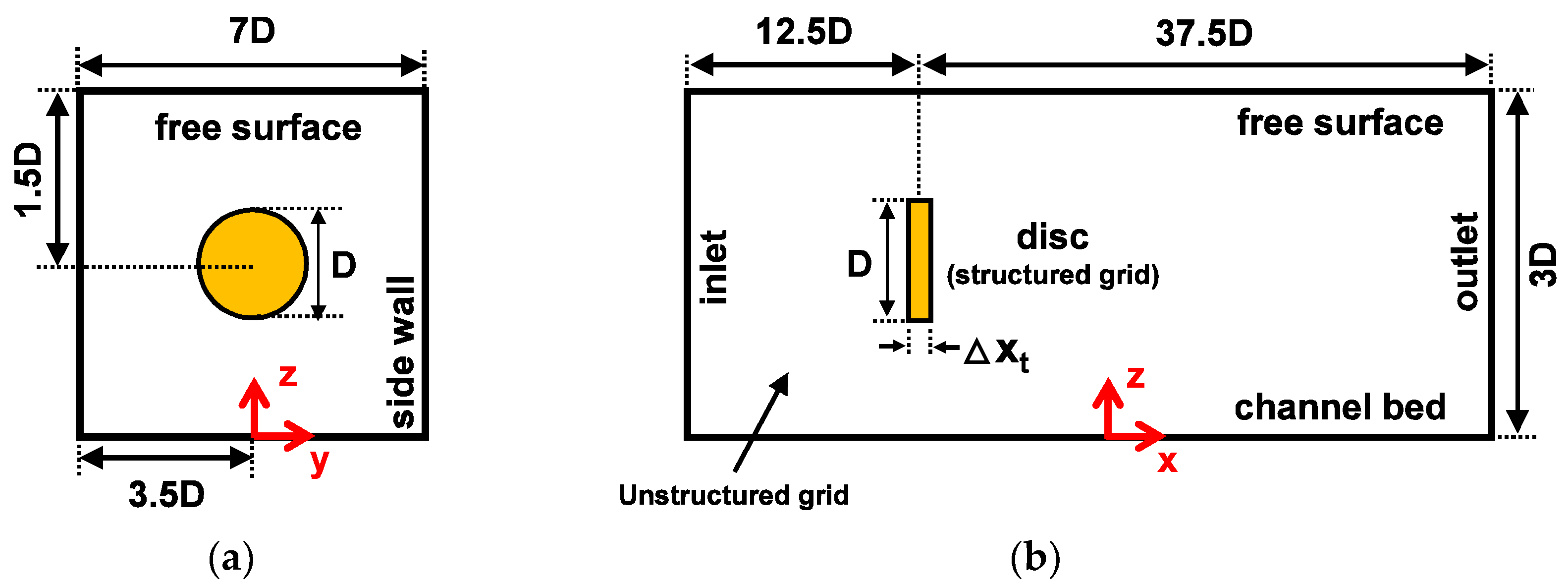
The turbine arrangement and the overall dimensions of the domain used in this study is presented in Figure 1, where the disc was located 250 m from the channel inlet. Additionally, its z and y axis centreline were fixed at a 30-m mid-depth and 70-m from the side wall.

(b)

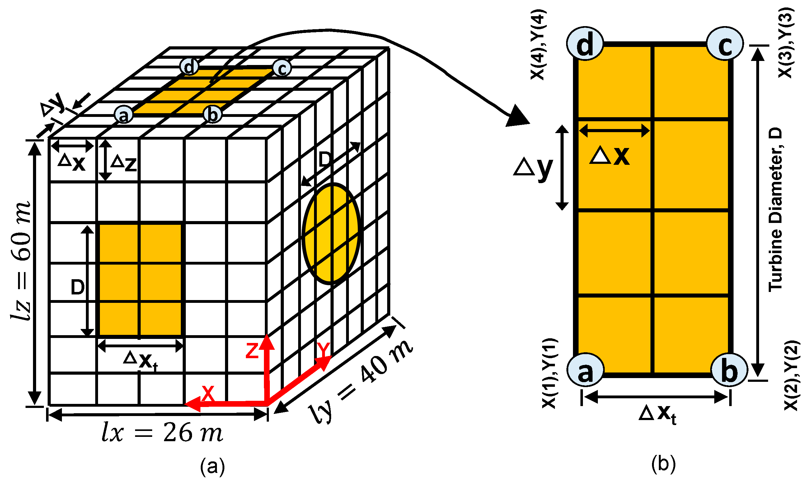
The use of a structured grid at the turbine position was chosen as it would allow for a better representation of the turbine shape, as well as maintaining the distance between nodes for refinement purposes. Figure 2 provides the graphical information on the dimensions and pertinent parameters concerning the implementation of the structured grid in the domain. The size of the structured grid (i.e., lx = 26 m, ly = 40 m and lz = 60 m) were deliberately set to be larger than the turbine diameter (D = 20 m) and its width ($\mathsf{\Delta }{x}_t=$ 2 m) to allow for numerical tolerance upon the execution of the momentum sink in the TRISOU subroutine. The grid element spacing within this structured grid are denoted by $\mathsf{\Delta }x$, $\mathsf{\Delta }y$ and Δz in the x, y, and z directions, respectively. For the simulations, lx, ly, and lz were kept constant, but the dimensions of $\mathsf{\Delta }x$, $\mathsf{\Delta }y$, and $\mathsf{\Delta }z$ were varied and their impact on the wake characteristics was investigated and the results are presented in Section 4.

(c)

The location of the disc (i.e., the turbine) in the domain was specified by four nodes in the horizontal plane (see Figure 2a), denoted as a, b, c, and d, which will act as the enclosure for the turbine. The coordinate of each node was represented by a pair of x and y. The distance between $y\left(4\right)$ and $y\left(1\right)$ refers to the turbine diameter, D, while the distance between $x\left(1\right)$ and $x\left(2\right)$ corresponds to the disc thickness, $\mathsf{\Delta }{x}_t$.

(d)

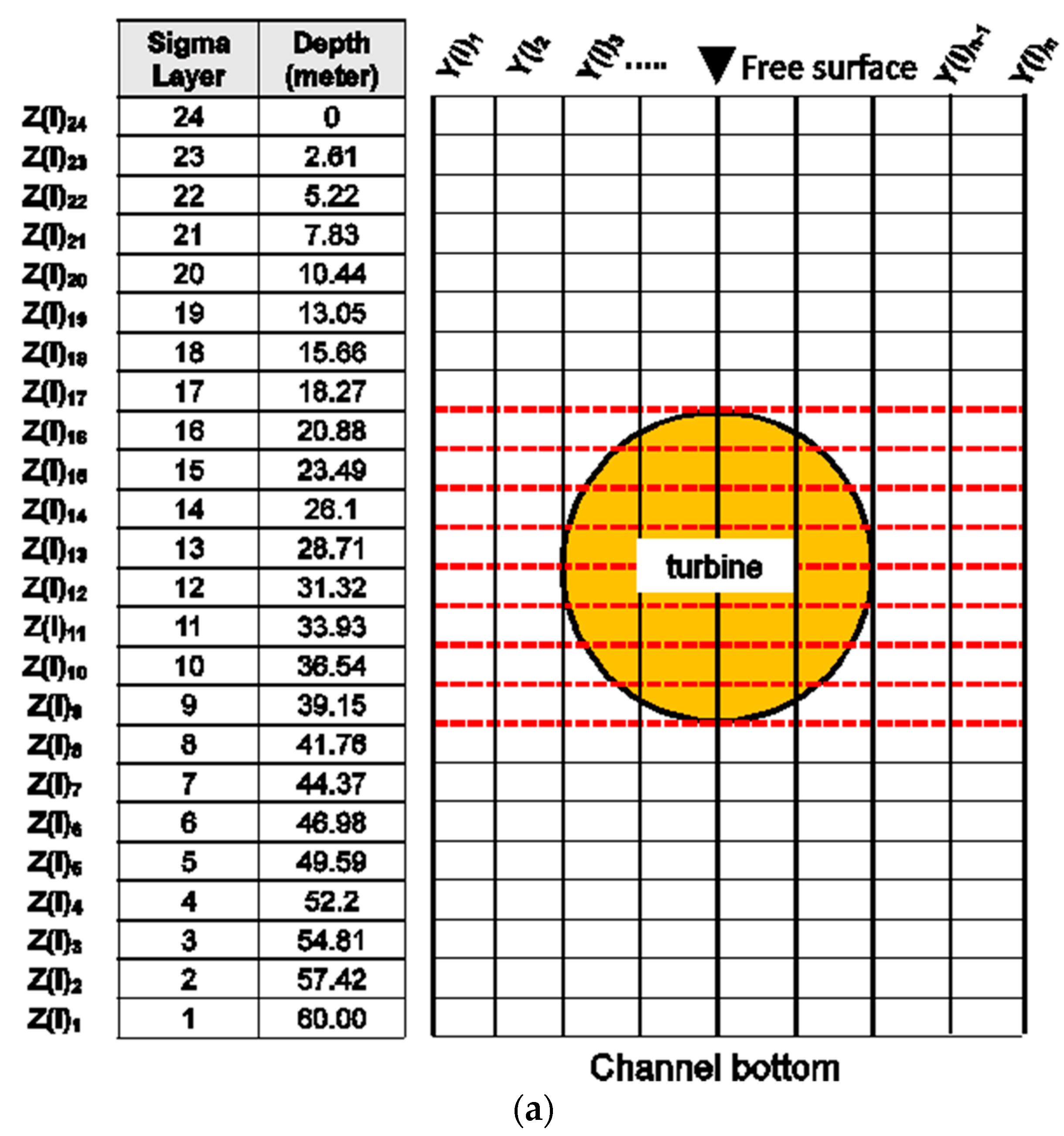
Although several mesh transformation options are available in the Telemac3D module, the sigma coordinate system was chosen to represent the depth due to its simplicity, as shown in Figure 3a. In fact, the interval between the vertical planes, $\mathsf{\Delta }z$ as well as the mesh density in the y direction, $\mathsf{\Delta }y$ must be carefully selected since the intersections between the z and y axis nodes will determine the accuracy of disc frame. Coarser mesh density in both the y and z axis will result in a limited number of nodes available within the disc surface area, as shown in Figure 3b. Whereas, Figure 3c portrays unbalanced concentration of the nodes when one of the axis uses a very fine grid resolution compare to the other. Section 4.3.2 will elaborate further on this subject matter.

(e)

Once the optimal resolution for both $\mathsf{\Delta }z$ and $\mathsf{\Delta }y$ was established, the momentum source term (see Equation (6)) was applied into the model through the existing nodes within the 10-m radius from the disc centre, Figure 3b. For this purpose, Equation (9) was employed to locate all the relevant nodes that formulate the disc’s 20-m frame.

$$Turbineradius,r=\sqrt{{\left(Y_i-Y_c\right)}^2+{\left(Z{\left(I\right)}_i-Z_c\right)}^2}$$

(9)

$$Y_c=\frac{y\left(4\right)-y\left(1\right)}{2}$$

(10)

where $Y_i$ refers to the node in y orientation within the turbine enclosure, $Y_c$ is the turbine centreline in the y direction (70 m), $Z{\left(I\right)}_i$ is the vertical plane in z direction where i = 24 sigma layers, and $Z_c$ is the depth where the turbine centre is located (30 m).

3.2. Model Set-Up

For a realistic modelling condition of a full-size turbine, the authors refer to the report by Legrand [22] to get an idea of the generic characteristic of a tidal energy device. A 20-m diameter disc was used in this study since it is a reasonable size for a standard horizontal axis turbine in operation. Moreover, the deployment of devices at any particular location is site and depth dependent, where a depth between 40 m to 80 m are often quoted. For this numerical study, the flow at the free surface and the channel depth was set to 3 m/s and 60 m respectively to resemble the general condition of the Pentland Firth area [23]. The disc z-axis centreline is positioned at the mid depth (30 m) to allow for a sufficient bottom clearance to minimize turbulence and shear loading from the bottom boundary layer. Also, the actuator disc is placed 250 m from the channel inlet to ensure that the flow is fully developed upon reaching the turbine area.

The resistance coefficient, K is one of the most important variables in simulating the actuator disc since it characterises the thrust exerted by the turbine on the flow. Changing the value of K will invariably influence the wake downstream of the disc. The relationship between C_T and K has been shown previously using Equation (7). In this paper, K is set to a constant value of 2, which correspond to C_T = 0.89.

As mentioned previously, structured grid was imposed at the location of the turbine to give an accurate illustration of the disc shape. Conversely, unstructured mesh was used for the surrounding area with a maximum edge length of 10 m, while the edge growth ratio was set to 1.1 for smoother mesh distribution. Figure 4 displays the unstructured mesh used in the computational domain, and it also shows the location of structured grid where the turbine is housed. Note that unstructured mesh was applied for the outer region since it is more flexible in capturing complex coastline features for realistic ocean scale simulations. The number of mesh elements vary significantly, depending on the value of $\mathsf{\Delta }x$, $\mathsf{\Delta }y$ and Δz chosen for different models, ranging from 70,000 to more than 900,000 cells. The model was run for 1500 s, at which the results indicated that a steady state had been achieved. The time step used for the simulation was ensured to meet the CFL (Courant–Friedrichs–Lewy) criterion. The simulations were computed on an i7 3770 quad core computer with 16 GB memory, and depending on test cases, it took between 3–5 h for simulations to be completed.

3.3. Boundary Condition

A constant volume flowrate, Q of 21,840 m³/s was imposed at the channel inlet, where Q is equal to the surface area of the inlet (60 m × 140 m) multiply by the mean flow velocity (2.6 m/s). Next, the downstream boundary was set to equal the channel water depth of 60 m to enable flow continuity. Initial condition was set to “PARTICULAR” (an option available in Telemac3D for defining the initial condition), where the initial depth of 60 m was specified in the CONDIM subroutine. A commonly used method of defining inflow velocities is to use a power-law (1/nth) profile. Although it is possible to use any value for n to approximate the flow conditions, a comparison of several values for n was considered to be beyond the scope of this study. Thus, the vertical velocity profile in the domain was imposed using one of the most commonly used power laws, 1/7th, so as to be similar to a full-scale tidal site [24]. In addition, the Chezy formulation with a friction coefficient of 44 was applied to the bottom to reduce the flow velocity as well as to increase the shear near the bed. This value was chosen as it has been used previously in [25] to represent the bottom roughness in the Pentland Firth region. Although not shown in the present paper, a wide range of friction coefficient values have been examined, and their influence on the model’s output were shown to be negligible. In this study, both hydrostatic and non-hydrostatic code were tested, and are discussed in Section 4.5.

Boundary condition on the bottom was set to a Neumann condition, which is a slip boundary condition. An attempt to implement a non-slip condition, where the bottom velocities can be set to 0 was not possible in this study since the model would require a very fine mesh near the bottom level to satisfy the wall function. Wall function, $y^{+}$ is a non-dimensional distance used to describe the ratio between the turbulent and laminar influences in a grid cell, as well as to indicate the mesh refinement for near wall region in a flow model [26]. The rationale behind the wall function is to reduce computational time and also to increase both numerical stability and convergence speed in resolving the boundary layers. However, because of the strong gradients of the flow and also turbulence variables that exist in the viscous layer, highly-refined grids are needed near the bottom [27]. Small-scale models are known to use a no-slip wall at the bed (refer to References [4,5,7]) since it is still computationally feasible to satisfy the $y^{+}$ requirement. Nonetheless, the flow details in the boundary layer were not of specific interest in this paper. Further, the use of a very fine vertical resolution (e.g., 50 planes or more) for modelling a full-size turbine is both impractical and not computationally feasible without the use of computer cluster.

3.4. Turbulence Input

Different values of stream wise turbulence intensities, TI, have been reported in the literature for both in situ measurements and flume experiments, which ranges from 3% to 25% [19,28,29,30,31,32,33,34,35,36]. TI is defined as the ratio of the turbulent fluctuations, ${\sigma }_i$ of the velocity fluctuation components (i = u, v, w) to the mean streamwise velocity of each sample, $\overline{U}$, and is one of the most common metrics utilised to quantify turbulence [37]. This parameter provides a quantification of the magnitude of the turbulent fluctuations and is considered to be a dominant driver of the fatigue loads on tidal turbine blades [38]. In Telemac, the equations for the standard k-$\epsilon$ turbulence model is given as follows:

$$\frac{\partial k}{\partial t}+U\frac{\partial k}{\partial x}+V\frac{\partial k}{\partial y}+W\frac{\partial k}{\partial z}=\frac{\partial }{\partial x}\left(\frac{v_t}{{\sigma }_k}\frac{\partial k}{\partial x}\right)+\frac{\partial }{\partial y}\left(\frac{v_t}{{\sigma }_k}\frac{\partial k}{\partial y}\right)+\frac{\partial }{\partial z}\left(\frac{v_t}{{\sigma }_k}\frac{\partial k}{\partial z}\right)+P-G-\epsilon$$

(11)

$$\begin{gathered} \frac{\partial \epsilon }{\partial t}+U\frac{\partial \epsilon }{\partial x}+V\frac{\partial \epsilon }{\partial y}+W\frac{\partial \epsilon }{\partial z}=\frac{\partial }{\partial x}\left(\frac{v_t}{{\sigma }_{\epsilon }}\frac{\partial \epsilon }{\partial x}\right)+\frac{\partial }{\partial y}\left(\frac{v_t}{{\sigma }_{\epsilon }}\frac{\partial \epsilon }{\partial y}\right)+\frac{\partial }{\partial z}\left(\frac{v_t}{{\sigma }_{\epsilon }}\frac{\partial \epsilon }{\partial z}\right) \\ +C_{\iota \epsilon }\frac{\epsilon }{k}\left[P+\left(1-C_{3\epsilon }\right)G\right]-C_{2\epsilon }\frac{{\epsilon }^2}{k} \end{gathered}$$

(12)

where

$k=\frac{1}{2}\overline{u_i^{\prime }{u}_i^{\prime }}$ denotes the turbulent kinetic energy of the fluid,

$u_i^{\prime }=U_i-\overline{u_i}$ denotes the ith component of the fluctuation of the velocity (u, v, w),

$\epsilon =\upsilon \overline{\frac{\partial u_i^{\prime }}{\partial x_j}\frac{\partial u_i^{\prime }}{\partial x_j}}$ is the dissipation of turbulent kinetic energy,

$P={\nu }_t\left(\frac{\partial \overline{U_i}}{\partial x_j}+\frac{\partial \overline{U_j}}{\partial x_i}\right)\frac{\partial \overline{U_i}}{\partial x_j}$ is a turbulent energy production term, in which ${\nu }_t=C_{\mu }\frac{k^2}{\epsilon }$

and $G=-\frac{{\nu }_t}{P{r}_t}\frac{g}{\rho }\frac{\partial \rho }{\partial z}$ is a source term due to the gravitational forces.

To properly validate the numerical simulations, the imposed turbulence intensity on the models should be as close as to the one used by Harrison et al. [5] in their experimental work. Using an online tool [39] to extract the published data from Reference [5], the measured turbulence intensities rate at the domain inlet can be approximated to vary from 5 to 15%. With the value of TI now known, the k-$\epsilon$ turbulence model can be adopted to define the turbulence at the channel inlet, where the turbulent kinetic energy, k and energy dissipation, $\epsilon$ are calculated using Equations (13) and (14):

$$k=\frac{3}{2}T{I}^2{U}^2$$

(13)

$$\epsilon =C_{\mu }^{3/4}\frac{k^{3/2}}{l}$$

(14)

TI is the turbulence intensity rate of 5%, U refers to the velocity across the water column that follows the 1/7th power law, $C_{\mu }$ is a dimensionless constant, equal to 0.09, and $l$ is the turbulence length scale. In the study, the value of $l$ was set to 20 m, which corresponded to one-third of the channel depth.

Table 2. Default values of the numerical parameters employed in the simulation of the actuator disc.

Numerical Parameters	Input/Values
Law of the bottom friction and the corresponding friction coefficient	Chezy (44)
Turbulence model	k-$\epsilon$ turbulence models
Hydrostatic assumption	True
Initial condition	“PARTICULAR” where the initial elevation is set to 60 m
Vertical resolutions	24 sigma layers
Boundary condition on the bottom	Slip condition
Boundary forcing	Inlet: prescribed flowrate, Q = 21,840 m3/s Outlet: prescribed elevation, H = 60 m
Resistance coefficient, K	2 (corresponding to CT = 0.89)

summarises the input/value of the parameters of the actuator disc model adopted in the numerical simulations.

4. Models’ Sensitivity and Validation

4.1. Validation Metric

Appropriate metrics need to be chosen for the model–data comparisons. As this study employs a full-size turbine for the model, a dimensionless metric was needed for the validation against physical scale data. All parameters were made dimensionless by dividing it by a characteristic homogeneous quantity. A commonly used method employed to characterize the wake recovery is the rotor velocity deficit, $U_{deficit}$ (see Equation (15)). $U_{wake}$ refers to the velocity at any points downstream of the disc, while $U_{freestream}$ is the unperturbed flow velocity. In this study, $U_{freestream}$ corresponds to 3 m/s as defined by the maximum velocity of the incoming stream into the channel. Next, turbulence intensity (TI) has been chosen as the benchmark quantity for turbulence behaviours (see Equation (16)).

$$U_{deficit}=1-\frac{U_{wake}}{U_{freestream}}$$

(15)

$$TI=\frac{\sqrt{\frac{2}{3}k}}{U}$$

(16)

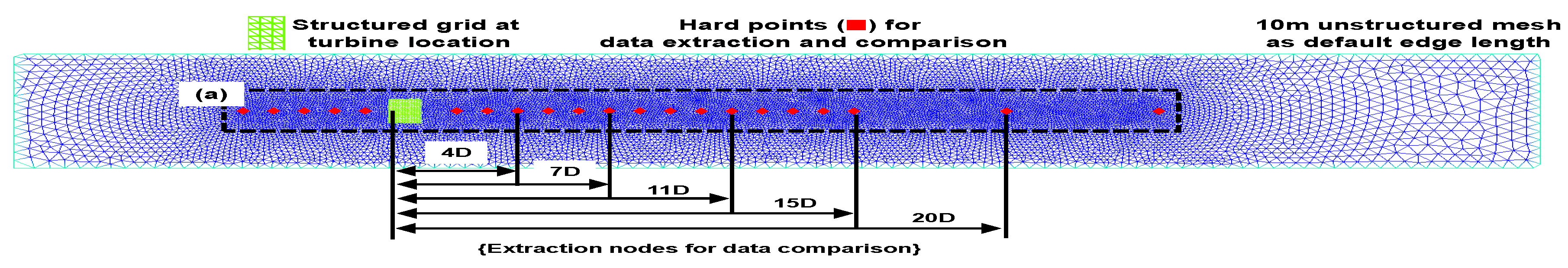
To examine the accuracy of the 3D models, focus will be placed on the modelled velocity reduction as well as the turbulence characteristics along the actuator disc centreline. The centreline is defined as the horizontal line that passes through the turbine centre along the x orientation of the flow direction. For this study, the z and y disc centreline axis were located at 30-m mid-depth, and at 70-m mid-channel width, respectively. Furthermore, to facilitate data extraction and for comparison purposes, hard points were applied into the geometry mesh during pre-processing stage to establish the positions of the fixed nodes within the domain. Figure 4 demonstrates the implementation of the hard points (specified by the red nodes) along the x centreline orientation at a desired longitudinal distance (in terms of turbine diameter, D).

4.2. Mesh Dependence Test

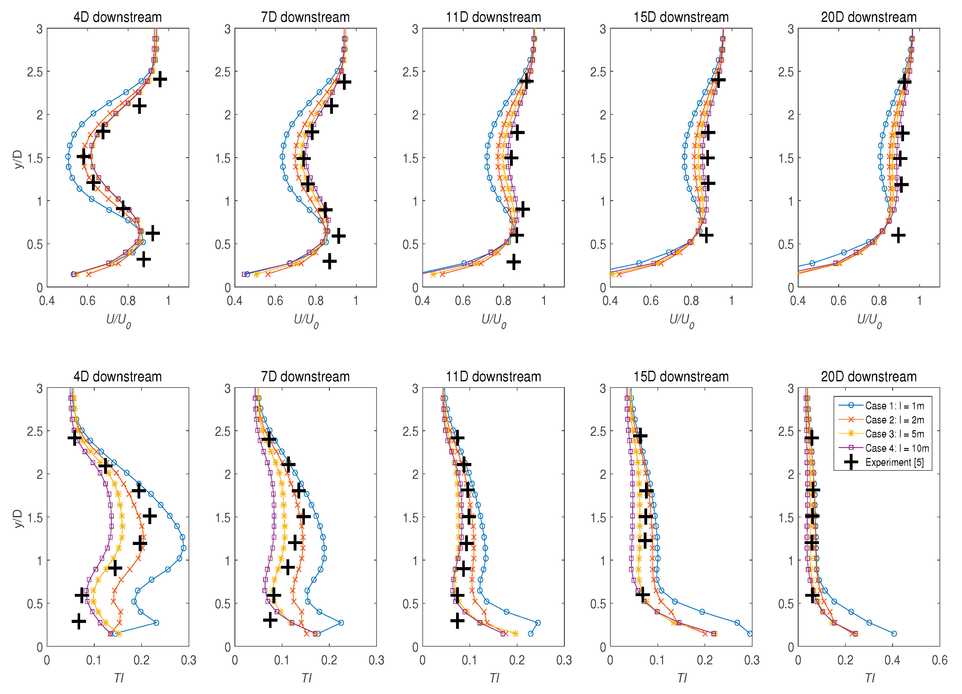
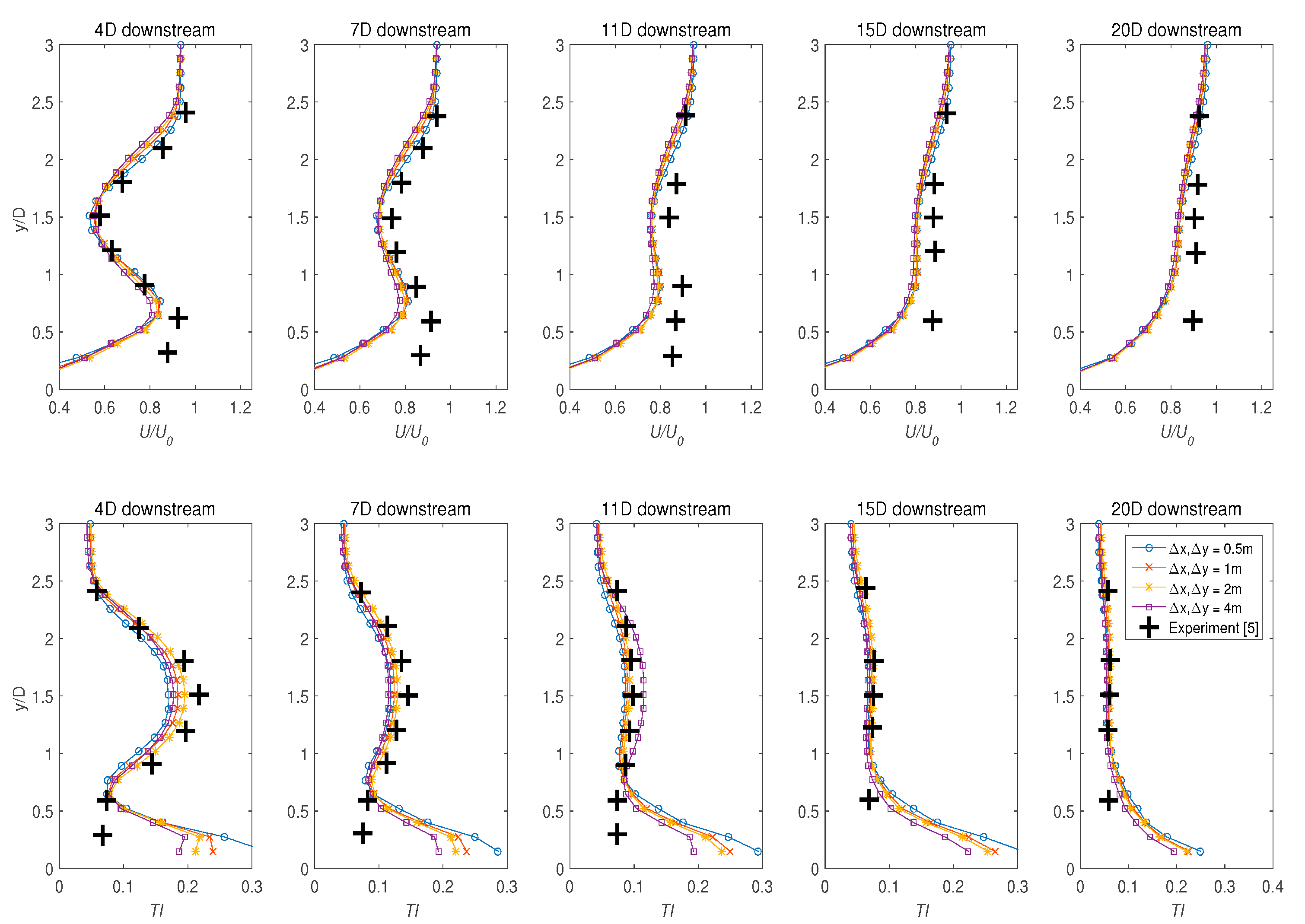
Because of the approximations and averaging used in the RANS equations, the size as well as the number of cells in any given CFD domain can directly affect the results of a numerical model. A larger number of cells may result in a more accurate solution to a problem for a given set of boundary conditions and solver settings. However, increasing mesh density also requires greater processing time. In order to verify the robustness of the unstructured mesh used in the model, four mesh (i.e., the dimension of the edge length of the unstructured mesh) with varying resolutions were tested; Case 1 = 1 m, Case 2 = 2 m, Case 3 = 5 m, and Case 4 = 10 m. The refinement zone starts at 5D upstream of the disc, continues up to 25D downstream as this region is selected for data extraction for comparisons with published literature. Figure 4 outlines the mesh refinement zone as well as the fixed nodes that are used in validating the model. It was decided to extract the output parameters at five locations of the computational domains, which are located at 4D, 7D, 11D, 15D, and 20D from the centre of the turbine, where D is the rotor diameter (refer to Figure 4). Elsewhere, a default edge length of 10 m was applied. For this mesh dependency test, the structured grid at the turbine area was constructed using elements of size $\mathsf{\Delta }x$ = 2 m and $\mathsf{\Delta }y$ = 2 m for all models, while the disc thickness, $\mathsf{\Delta }{x}_t$ was set to 2 m. Also, the model was run using only the hydrostatic assumption.

Table 3. Grid dependency study.

Refinement Details		Centreline Velocity at Various Longitudinal Positions from Actuator Disc (m/s)
Mesh Size	Number of Elements	5D Upstream	4D Downstream	7D Downstream	11D Downstream	20D Downstream
Case 1 (1 m)	925,536	2.683	1.515	1.903	2.153	2.418
Case 2 (2 m)	316,584	2.680	1.735	2.092	2.315	2.554
Case 3 (5 m)	101,496	2.690	1.853	2.186	2.391	2.600
Case 4 (10 m)	72,936	2.694	1.846	2.247	2.464	2.659

highlights the models used in the grid dependency study, where four refinements values were tested. The most refined model (Case 1) consists the highest number of elements at 925,536, while the model which has the minimal resolution (Case 4) comprises the least number of elements at about 70,000. The velocity data were then extracted at five distinct nodes (refer to Figure 4) and are listed in Table 3. The results, in general, indicate that increasing mesh density decreases the velocity; however, the difference was not high. This observation is supported by Figure 5 which compares the models’ velocity reduction (top plots) and TI (bottom graphs) against the laboratory measurement data from [5]. Overall, the results show that all models manage to produce velocities more or less the same as the experimental values behind a disc. Interestingly, although a higher resolution domain was expected to give a better correlation against the experimental data, contradictory results were obtained. That is, the 1 m grid refinement seems to overestimate the velocity reduction by almost 10% in the near wake, before declining slowly in the far wake regions. Likewise, these scenarios are also reflected in the observation of TI, where the 1 m model appears to amplify the turbulence below the disc centreline in the 4D and 7D regions. Several possible reasons may contribute to this behaviour; a higher resolution model contains a large number of points in the domain, which signify that the cells are more sensitive to the flow characteristics in the surrounding region.

On the other hand, the 2 m mesh refinement (Case 2) agrees well with the measurement data, although a slightly higher velocity was observed in the far wake regions. Meanwhile, models with a resolution of 5 m and 10 m were shown to be less accurate in the TI prediction in comparison with experimental data, where both models significantly underestimated the TI in the 4D and 7D regions. These results illustrate that the coarser resolution models fail to properly represent the flow-rotor interaction, indicating that the models output (i.e., velocity, TI) is susceptible to changes in mesh density. To conclude, the use of a very fine mesh alongside hydrostatic assumption may not necessarily provide superior numerical output as demonstrated by test Case 1 using the 1 m mesh density. Consequently, as the simulation results for the 2 m mesh (Case 2) closely matched with the measurement, this has been implemented as the optimal mesh discretisation for the following simulations.

4.3. Sensitivity of the Structured Grid at Turbine Location

A structured grid was employed to define the area of the actuator disc for two key reasons: one to facilitate in identifying the nodes for momentum sink implementation and the other to improve the accuracy of the approximated turbine forces by correctly asserting the physical shape of the disc. In this section, the influence of turbine grids resolution (i.e., $\mathsf{\Delta }x\mathrm{and}\mathsf{\Delta }y$) on the wake characteristics of a full-scale actuator disc is explored.

4.3.1. Influence of the Disc Thickness, $\mathsf{\Delta }{x}_t$

For the test, a 2 m by 2 m ($\mathsf{\Delta }x\&\mathsf{\Delta }y)$ structured grid was embedded into the unstructured mesh domain where the turbine was located. The models were then run using three different turbine thickness values, $\mathsf{\Delta }{x}_t=$2 m, 4 m, and 8 m. For clarification, when $\mathsf{\Delta }{x}_t$ is set to 4 m, the flow will have to pass through two $\mathsf{\Delta }x$ grid cells (each cell is 2 m as displayed in Figure 2) in the x direction where the momentum source terms will determine the forces exerted by the turbine. Figure 6 illustrates the comparison of the measurement data for the above three values of $\mathsf{\Delta }{x}_t$.

Interestingly, the results show that the thickness of the actuator disc had negligible influences on both the downstream wake, as well as the turbulence intensities. Although not shown here, similar observations were also apparent when the $\mathsf{\Delta }x\mathrm{and}\mathsf{\Delta }y$ values were changed to other than 2 m resolutions. Therefore, it can be deduced that the downstream wakes and turbulences behind the turbine are independent of the actuator disc thickness.

4.3.2. Resolution of the Structured Grid ($\mathsf{\Delta }x\&\mathsf{\Delta }y$)

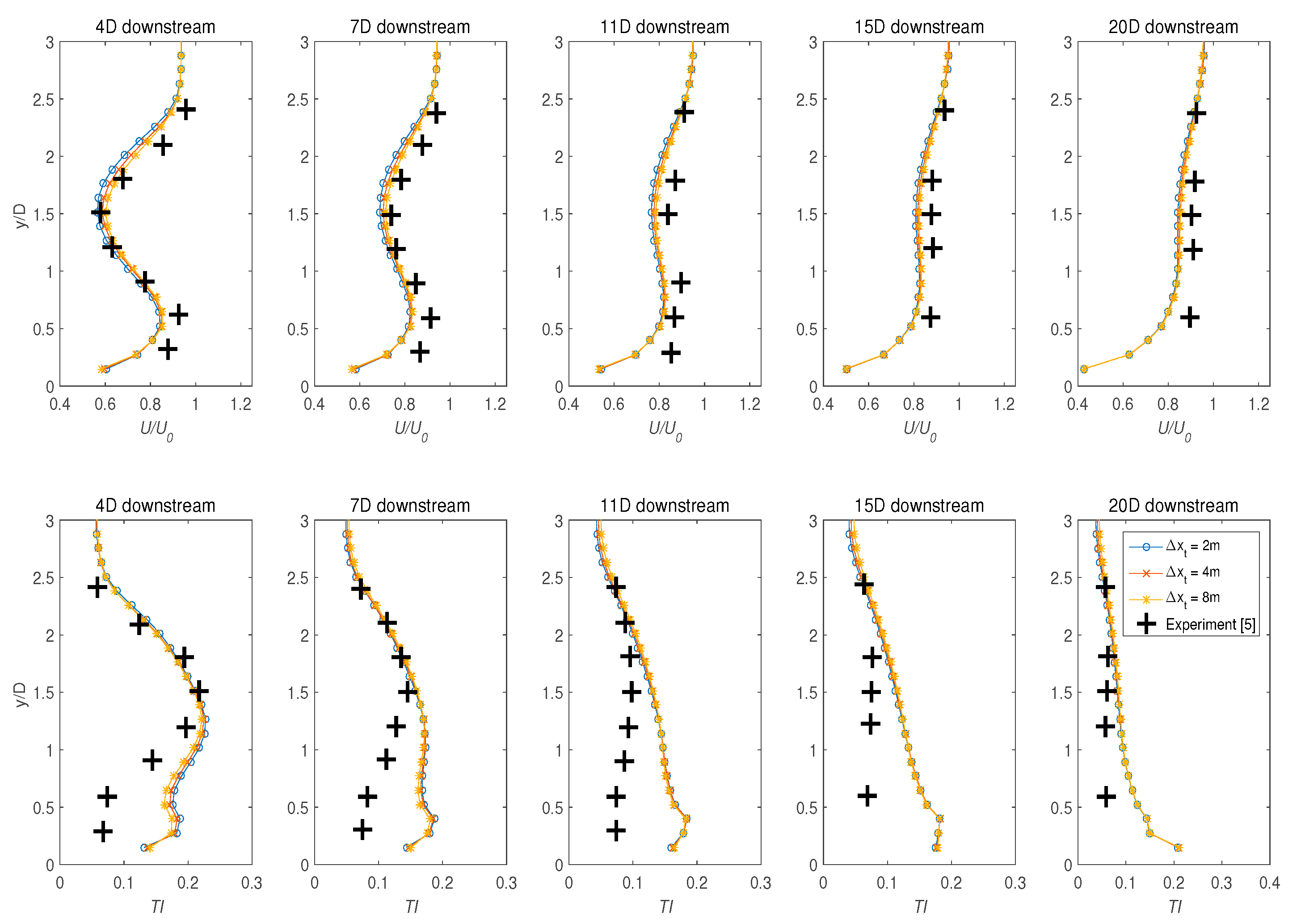
The interaction between the resistance loss coefficient ($K/\mathsf{\Delta }{x}_t$) and the resolution of the structured grids ($\mathsf{\Delta }x\mathrm{and}\mathsf{\Delta }y$) at the actuator disc location is explored here. As previously mentioned, K is the constant resistance coefficient which corresponds to the experimental values of $C_T.$ As the flow progresses through the turbine swept area, it expands and accelerates around the edge or “width” of the disc. In the numerical model, the flow passing through the width or thickness of the turbine literally means that it is travelling across specific nodes in the x direction as defined by the enclosure of the disc. For a very fine mesh with constant $\mathsf{\Delta }{x}_t$, the source term will be applied to a larger set of nodes when compared to a coarser grid. To examine the relationship between the nodes and their impact on the wake characteristic, four structured grids with various densities were created and examined. The lowest resolution of $\mathsf{\Delta }x$ and $\mathsf{\Delta }y$ tested was 4 m, while the most refined was set to 0.5 m. Figure 7 highlights enticing differences between the four models using a constant $\mathsf{\Delta }{x}_t$ of 2 m. Even though $\mathsf{\Delta }{x}_t$ was found to have no impact on the results as noticed in Section 4.3.1, we selected 2 m thickness here as this would be close to projected thickness of a turbine.

The model with the highest grid density (0.5 m) appeared to overestimate the velocity reduction behind the disc by almost 20% in the near wake region and continued to do so further downstream with a larger velocity deficit compared to other models. The same trend was also observed for the model with a 1 m grid, although the extent of the velocity deficit was less pronounced as the flow started to reach homogeneity. In contrast, models utilizing the 2 m and 4 m grids seemed to be able to simulate the flow-rotor interaction accordingly and compared well with the experimental data. With turbulence intensities, since the 1 m grid produced a greater velocity deficit in the near wake region, this was reflected accordingly in the turbulence plots, where the intensities were less profound behind the disc due to wake mixing. A variation of TI up to 5% is seen for the case of 4D regions, then slowly recovers before matching other models at 15D downstream. However, a different trend is noticed for the 4 m grid model, as it shows some discrepancies for the TI in the near region, although it is not as dominant as the 0.5 m model.

The results presented in Figure 7 offers interesting insights for discussions. A less accurate output is expected from a coarser grid due to a limited (albeit uniformly scattered) number of nodes within the turbine enclosure as exemplified by Figure 3b. Conversely, one would have thought that the simulation output could probably be improved by using a very fine mesh, although it appears that this is not always the case based on the results attained. As the density of $\mathsf{\Delta }x\mathrm{and}\mathsf{\Delta }y$ increases, the nodes that render the turbine swept area, as well as the turbine width will also increase proportionally, as illustrated in Figure 3c. This figure clearly shows an uneven distribution of the nodes at the face of the actuator disc for a higher density model, where they are concentrated prominently at the mid-quarter of the disc. Since increasing the mesh density only applies in the x and y directions, the top and bottom edges were devoid of nodes. As a result, the implementation of the momentum term would only be directed at the centre of the turbine, which consequently will cause inaccuracy in the approximation of the turbine force, as evidenced from the plots in Figure 7.

To solve this, it is recommended that the vertical resolution should also be increased when a fine mesh is employed so that uniform node distribution can be achieved. Nonetheless, increasing the vertical density while using a very fine grid will undoubtedly increase the computational resources, especially when running a large-scale simulation. Thus, finding an optimal ratio for the mesh density and vertical resolution is crucial so that the implementation of the actuator disc can correctly approximate the thrust exerted by a turbine. Based upon the results presented in this case study, $\mathsf{\Delta }x=2\mathrm{m}$ and $\mathsf{\Delta }y=2\mathrm{m}$ were chosen as the optimal structured grid density since they provide numerical accuracy and computational balance needed for implementing the actuator disc.

4.3.3. Grid Resolution for $\mathsf{\Delta }y$

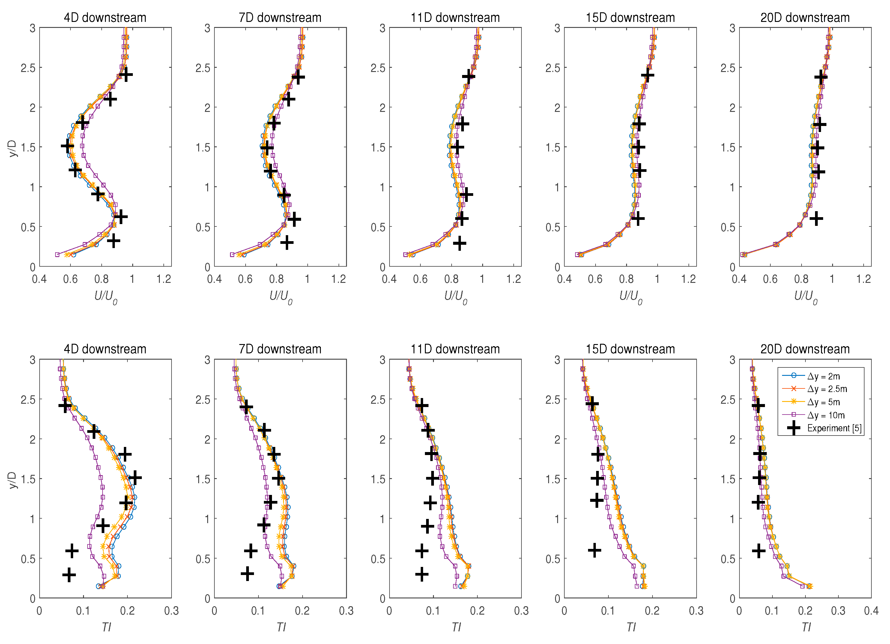
It is anticipated that models with coarser $\mathsf{\Delta }y$ will perform poorly when compared with a more refined density, since the force approximation only happens at a considerable node interval. To inspect this hypothesis, four $\mathsf{\Delta }y$ grids (2 m, 2.5 m, 5 m, and 10 m) were tested, while $\mathsf{\Delta }x$ and $\mathsf{\Delta }{x}_t$ were maintained at 2 m and 2 m, respectively. This hypothesis is substantiated and illustrated by the velocity plots in Figure 8, where the 10 m grid somewhat underestimated the velocity deficit in the near wake region. On the other hand, other $\mathsf{\Delta }y$ models showed good comparison against the laboratory measurements. Furthermore, since the coarser model ($\mathsf{\Delta }y=10\mathrm{m}$) contained a significantly smaller number of nodes, the model was unable to correctly approximate the thrust on the flow, resulting in a distinctly lower turbulence intensity between 4D and 7D downstream regions. The other models, however, showed a relatively similar characteristic for both $U_{deficit}$ and TI. Since the size of the disc adopted in this study is 20-m, an $\mathsf{\Delta }y$ value of 10 m or more might not be suitable to accurately model the actuator disc since the number of nodes available are not sufficient for approximating both the forces as well as the size of the swept area. To conclude, based on the results observed, $\mathsf{\Delta }y$ = 2 m is accepted as the optimal spacing in the y direction, and confirm the remarks made previously in Section 4.3.2.

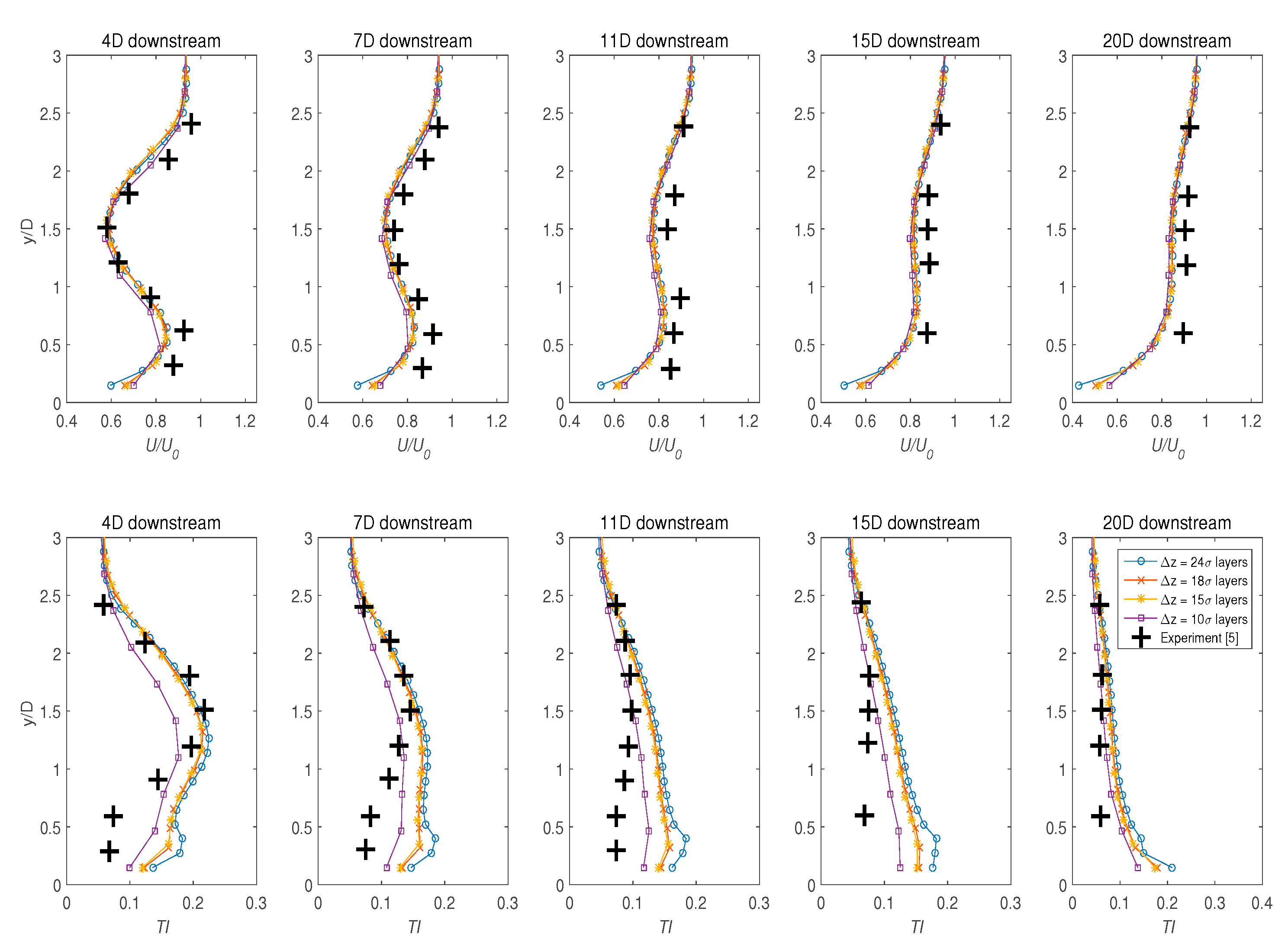
4.4. Sensitivity of the Vertical Resolutions, $\Delta z$

To investigate the influence of vertical resolutions on the model, four sigma ($\sigma$) layers were put to test; 24 (default value), 18, 15, and 10.

Table 4. Comparison of the vertical resolutions.

Sigma Layers	Distance between Planes (in Meter)	Number of Mesh Elements
24	2.61	317,928
18	3.53	238,446
15	4.29	198,705
10	6.66	132,470

provides the information of the models used in this study, where the largest (6.66 m) and smallest vertical interval (2.61 m) correspond to $10\sigma$ and 24$\sigma$ layers, respectively.

Further, based on the above observations in Section 4.2 and Section 4.3, $\mathsf{\Delta }x$ and $\mathsf{\Delta }y$ was set to 2 m for all models and $\mathsf{\Delta }{x}_t$ = 2 m was used. The simulated results are presented in Figure 9, where the model employing $10\sigma$ layers underestimated the TI as anticipated, since it had the least number of nodes to properly characterise the turbine swept area. However, it is quite interesting to see the same model was able to reproduce the velocity wake that matched the measurement results. One possible reason for this observation could be due to the hydrostatic assumption used in the model. Nonetheless, the poor turbulence correlation observed for the $10\sigma$ layers should be approached with caution. It shows that the region between 4D and 11D downstream of the disc was highly turbulent, and the flow fluctuations could not be accurately reproduced using planes with large vertical intervals. To get around this issue, instead of sigma layers, it was possible to utilise other types of mesh transformation for the distribution of vertical planes, such as by fixing planes at desired depths. With this option, the height of the vertical planes can be appropriately adapted to capture the influence of the disc on the flow. In brief, finding the optimal $\mathsf{\Delta }z$ values are crucial in achieving the balance between computational efficiency and numerical accuracy, more so for simulations involving a very large domain.

4.5. Hydrostatic vs. Non-Hydrostatic Pressure Models

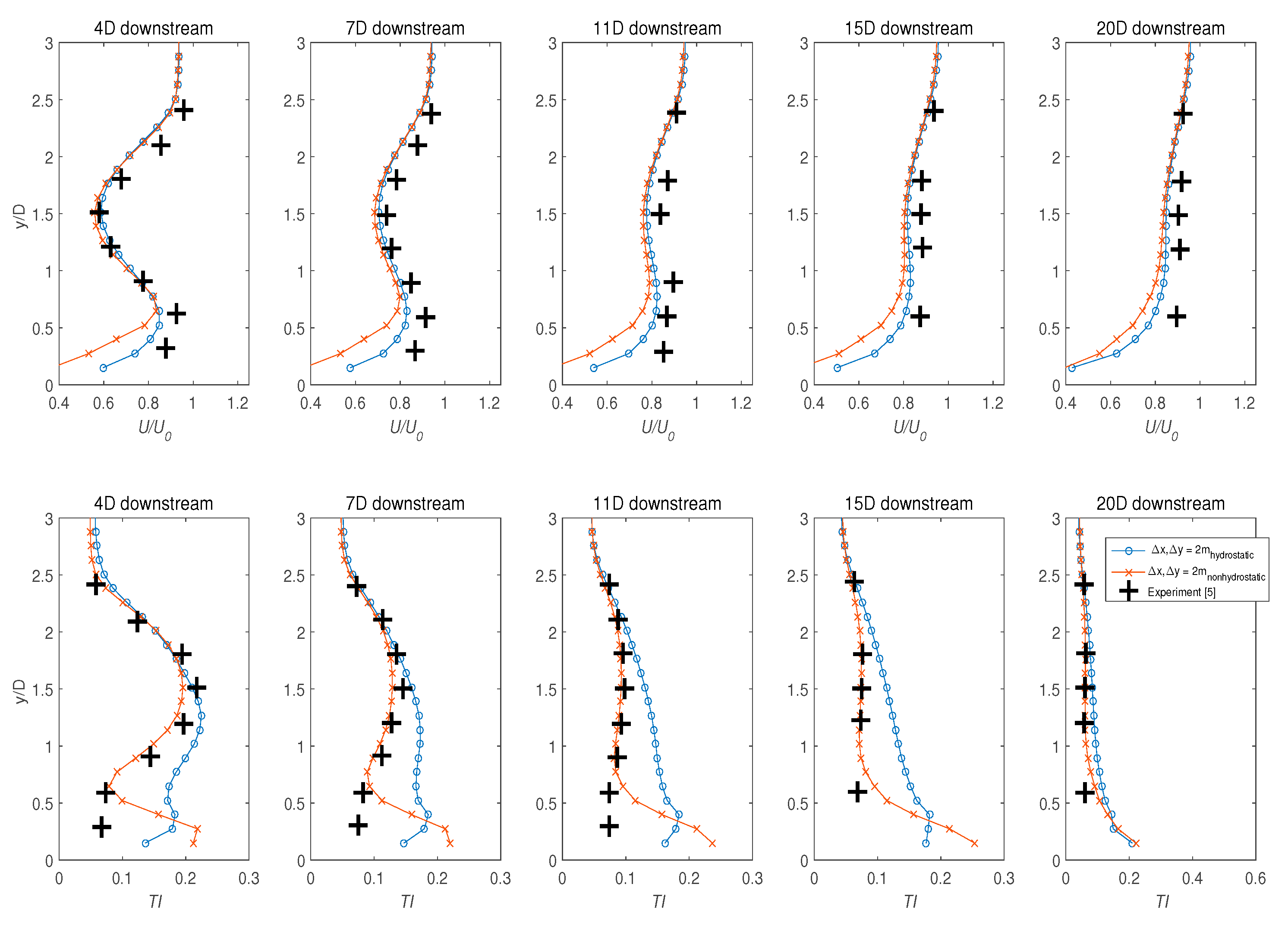
Telemac3D offers the choice of using either the hydrostatic or the non-hydrostatic pressure code. The hydrostatic pressure simplifies the vertical velocity (W) assumption, ignoring the diffusion, advection and other terms. Thus, the pressure at a point is the sum of weight of the water column and the atmospheric pressure at the surface. Conversely, the non-hydrostatic option solves the vertical velocity equation and is more computationally intensive. Similar with the 3D flow equations shown previously in Section 2.1 (Equations (1)–(3)), the non-hydrostatic assumption adopted in this section was computed by the following additional equation:

$$\frac{\partial W}{\partial t}+U\frac{\partial W}{\partial x}+V\frac{\partial W}{\partial y}+W\frac{\partial W}{\partial z}=-g\frac{\partial Z_s}{\partial z}+v\Delta \left(W\right)+F_Z$$

(17)

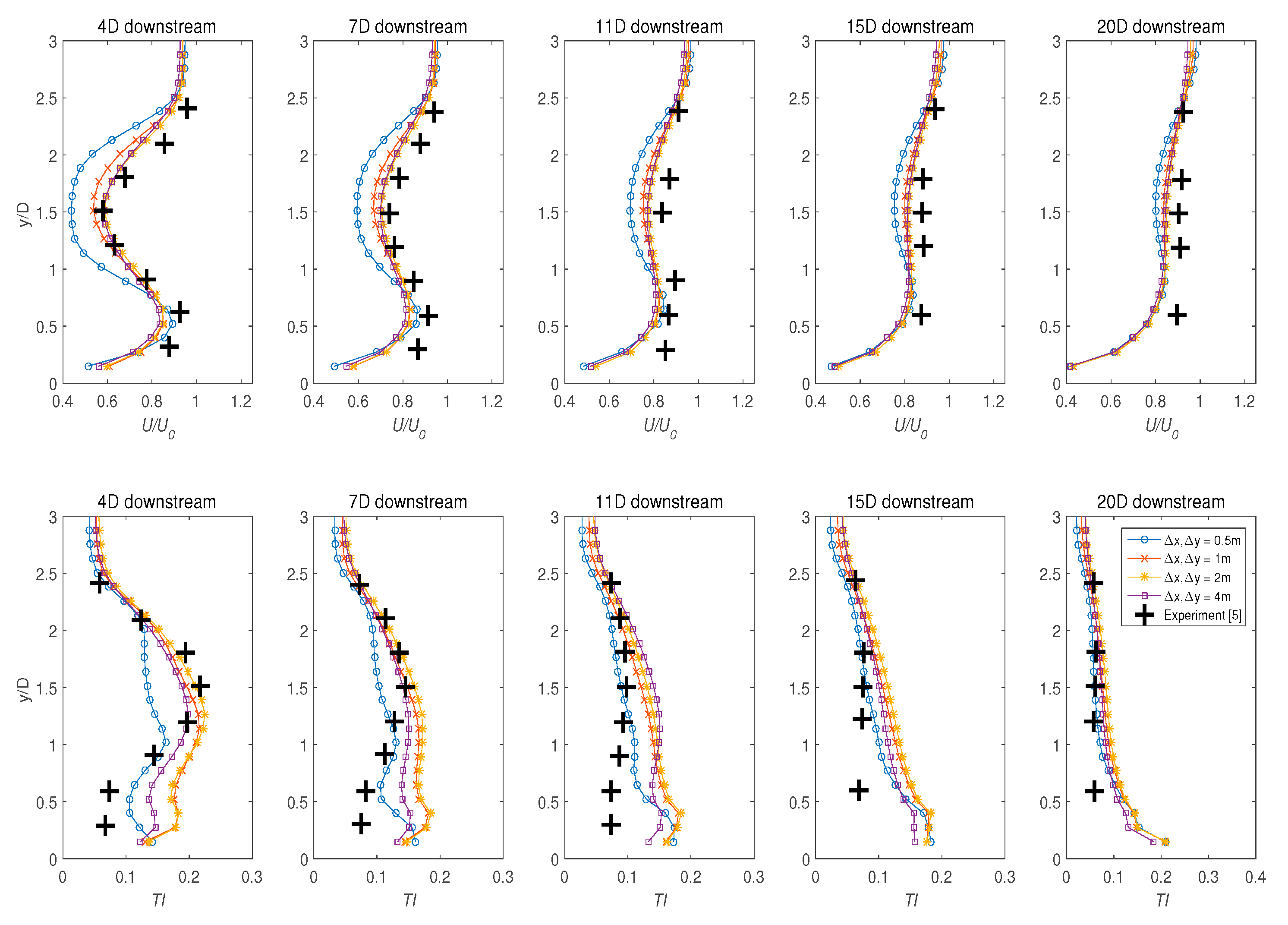
where W and F_z are the three-dimensional component of the velocity and sink term in the vertical direction, respectively. To examine the influence of both assumptions, models with $\mathsf{\Delta }x=2\mathrm{m},\mathsf{\Delta }y$ = 2 m, $\mathsf{\Delta }{x}_t=$ 2 m, and $\mathsf{\Delta }z$ = $24\sigma$ layers were simulated in both hydrostatic and non-hydrostatic solvers. Interestingly, the impact of the non-hydrostatic code on the velocity component was less pronounced as illustrated in Figure 10, where both models produced a nearly identical velocity reduction at 1.5 < y/D < 3. However, for the bottom half of the channel, the hydrostatic model somewhat showed a closer agreement with the measurement points than the model using the non-hydrostatic solver, especially in the near bed region. This was apparent in the 4D and 7D regions, where the wake velocity from the non-hydrostatic model showed a slight divergent from the measurement data approximately before y/D = 0.7. This trend continued to persist until the far wake regions, where the non-hydrostatic model slightly overestimated the wake velocity up to y/D = 1.5.

With regard to the turbulence intensity, the non-hydrostatic model demonstrated excellent agreement with the published data, where the solver seemed to be able to properly resolve the turbulence mixing from the near till far wake regions. In contrast, the computed TI from the hydrostatic model illustrated striking disparities from 4D to 20D wake regions, especially in the bottom half of the channel depth (see Figure 10). At 4D downstream of the disc, the hydrostatic model managed to produce good agreement with the measurement at 1.5 < y/D < 3 before gradually straying from the data points. Similar observations occur further downstream, where the differences in TIs between the two models were becoming more apparent. At 15D, the computed TI using the hydrostatic solver only matched the experimental data at 2.5 < y/D < 3, as the model displays an intensity variation of up to 10% against both the measured data and non-hydrostatic model. Ultimately, far downstream of the disc at 20D where the flow eventually reaches homogeneity, the two models presented an almost uniform turbulence characteristic.

To further validate these observations, simulations utilizing different set of structured densities $(\mathsf{\Delta }x,\mathsf{\Delta }y=0.5\mathrm{m},1\mathrm{m},2\mathrm{m},4\mathrm{m}$) were run in the non-hydrostatic formulation to examine the influence of the solvers on the wake characteristics. Figure 11 displays the results of these simulations. An excellent agreement against the experimental data was observed, regardless of the resolutions of the structured grid being tested. Moreover, the use of the non-hydrostatic code also eliminated the turbulence variations in the bottom half of the actuator disc, as previously observed in Figure 10 where the hydrostatic assumptions were employed. These findings demonstrate that the non-hydrostatic code has a significant influence in resolving the vertical turbulence mixing downstream of the disc, where the previously seen variations for both $U_{deficit}$ and TI from the hydrostatic models were remarkably corrected.

The comparisons between the two codes present compelling points for discussions. The output by the non-hydrostatic model exhibited close agreement with the measurement data as expected since it accounts for the gravitational acceleration as well as the w-velocity component, and thus is more accurate. Whereas the flow characteristics observed from the hydrostatic pressure code only matched the scale data for the velocity components, the turbulence comparisons differ greatly. Two possible reasons may be attributed to this observation. First, there existed no stringent guidelines as to what extent could the hydrostatic assumption be safely used for an actuator disc approximation in a simple channel case. A condition which allows for hydrostatic assumption in a system implies that the horizontal length scale is much greater than the water depth. Indeed, it might be possible that the horizontal length of the domain utilised in this study did not satisfy the optimal ratio for hydrodynamic pressure assumption.

Secondly, the turbulence in the flow may not have fully resolved as the non-slip criteria could not be implemented on the channel bed. The non-slip criteria require the use of a highly-refined mesh to resolve the size of the smallest eddy in the flow as it begins to transition from laminar to turbulence regime. And since the hydrostatic code ignores the advection and diffusion term, the eddies cannot be properly dissipated, and thus influencing the turbulence characteristic in the near wake. Indeed, as the highest turbulence intensity zone was observed in the immediate vicinity behind the disc and then slowly dissipated further downstream, the hydrostatic model can only reproduce the expected intensities in the far wake regions, as shown by the 20D downstream plot. For future references, it may be wise to increase the number of layers near the vicinity of the bed wall to account for the turbulence in the bottom half of the water column.

5. Conclusions

A study to examine the validity of the RANS actuator disc approach for a full-scale tidal turbine has been presented by comparing the model velocities and turbulence intensities against a laboratory measurement data sourced from literature. The numerical model Telemac3D was used for this purpose, and a detailed methodology in the implementation of the momentum source term was introduced and elaborated. The influence of: (i) unstructured mesh sizes used in the computational domain; (ii) change in the turbine thickness ($\mathsf{\Delta }{x}_t$); (iii) variation in the structured grid resolutions ($\mathsf{\Delta }x$ and $\mathsf{\Delta }y$) used to represent the turbine’s enclosure; (iv) variation in the vertical layer thickness ($\mathsf{\Delta }z$); and (v) the effect of hydrostatic and non-hydrostatic formulations on the model output parameters were explored. Key findings from this study are:

• The results demonstrated that the numerical model was highly sensitive to the mesh refinement upstream and downstream of the turbine, where coarser models tended to underestimate both the velocity retardation and TI.
• Altering the thickness of the turbine ($\mathsf{\Delta }{x}_t$) had negligible impact on the downstream wakes and turbulence mixings.
• Numerical accuracy of the model was found to be highly susceptible to changes in the grid density of the turbine enclosure. The optimal structured grid density of Δx = 2 m, and Δy = 2 m satisfactorily modelled both the velocity deficit and the TI.
• The importance of the grid spacing in y direction ($\mathsf{\Delta }y$) in characterising the thrust and also the shape of the disc was also highlighted.
• The influence of vertical resolutions (Δz) in representing the depth of the channel on the model was investigated to find a balance between computational efficiency and numerical accuracy. The findings indicated that appropriate adjustment on both the horizontal and vertical planes must be attained to accomplish the optimal ratio between the nodes resolution in both z and y orientation. Note that the optimal structured grid density found in this study was limited to the computational resources available to the authors. The methodology presented in this article, however, are still valid for a more refined grid implementation.
• The impact of the hydrostatic and non-hydrostatic pressure assumptions on the predicted output were examined, where both models exhibit nearly indistinguishable flow retardation characteristics behind the simulated disc. However, for the TI, only the non-hydrostatic model was able to match the experimental result, while the hydrostatic solver failed to properly resolve the turbulence mixing in the wake regions between 4D and 15D.

In summary, this paper provided a preliminary demonstration of the applicability of RANS actuator disc approach for a full-size tidal device. Future work will involve modelling several full-size turbines in an array using the methodology presented in this paper. Additionally, several other turbulence models, such as the k-ω and Reynolds Stress Models (RSM), may also be studied to understand their impact on the models’ output. Ultimately, the procedure followed in this study may hence be used as a guideline for the implementation of tidal turbines by the actuator disc method in regional scale simulations.

References

- Neill, S.P.; Litt, E.J.; Couch, S.J.; Davies, A.G. The impact of tidal stream turbines on large-scale sediment dynamics. Renew. Energy 2009, 34, 2803–2812. [Google Scholar] [CrossRef]
- Robins, P.E.; Neill, S.P.; Lewis, M.J. Impact of tidal-stream arrays in relation to the natural variability of sedimentary processes. Renew. Energy 2014, 72, 311–321. [Google Scholar] [CrossRef]
- Chatzirodou, A.; Karunarathna, H.; Mainland, S.; Firth, P.; Park, S. Impacts of tidal energy extraction on sea bed morphology. Coast. Eng. 2014, 1, 33. [Google Scholar] [CrossRef]
- Sun, X.; Chick, J.P.; Bryden, I.G. Laboratory-scale simulation of energy extraction from tidal currents. Renew. Energy 2008, 33, 1267–1274. [Google Scholar] [CrossRef]
- Harrison, M.E.; Batten, W.M.J.; Myers, L.E.; Bahaj, A.S. Comparison between CFD simulations and experiments for predicting the far wake of horizontal axis tidal turbines. IET Renew. Power Gener. 2010, 4, 613–627. [Google Scholar] [CrossRef]
- Adcock, T.A.; Draper, S.; Nishino, T. Tidal power generation–A review of hydrodynamic modelling. Proc. Inst. Mech. Eng. Part A J. Power Energy 2015, 299, 755–771. [Google Scholar] [CrossRef]
- Daly, T.; Myers, L.E.; Bahaj, A.S. Modelling of the flow field surrounding tidal turbine arrays for varying positions in a channel. Philosophical Trans. R. Soc. Lond. A Math. Phys. Eng. Sci. 2018, 371, 20120246. [Google Scholar] [CrossRef] [PubMed]
- Lartiga, C.; Crawford, C. Actuator Disk Modeling in Support of Tidal Turbine Rotor Testing. In Proceedings of the 3rd International Conference on Ocean Energy, Bilbao, Spain, 6–8 October 2010; pp. 1–6. [Google Scholar]
- Roc, T.; Conley, D.C.; Greaves, D. Methodology for tidal turbine representation in ocean circulation model. Renew. Energy 2013, 51, 448–464. [Google Scholar] [CrossRef] [Green Version]
- Nguyen, V.T.; Guillou, S.S.; Thiebot, J.; Cruz, A.S. Modelling turbulence with an Actuator Disk representing a tidal turbine. Renew. Energy 2016, 97, 625–635. [Google Scholar] [CrossRef]
- Hervouet, J.M. Hydrodynamics of Free Surface Flows: Modelling with the Finite Element Method; John Wiley & Sons: West Sussex, UK, 2007. [Google Scholar]
- Desombre, J. TELEMAC-3D OPERATING MANUAL (Release 6.2); EDF R&D: Paris, France, 2013. [Google Scholar]
- Hervouet, J.M.; Jankowski, J. Comparing numerical simulations of free surface flows using non-hydrostatic Navier-Stokes and Boussinesq equations. Electricité de France; Bauwesen der Universität Hannover; Unpublished work. 2000. [Google Scholar]
- Burton, T.; Jenkins, N.; Sharpe, D.; Bossanyi, E. Wind Energy Handbook; John Wiley & Sons: Weat Sussex, UK, 2011. [Google Scholar]
- Batten, W.M.J.; Harrison, M.E.; Bahaj, A.S. The accuracy of the actuator disc-RANS approach for predicting the performance and far wake of a horizontal axis tidal stream turbine. Philos. Trans. R. Soc. Lond. A Math. Phys. Eng. Sci. 2013, 371, 20120293. [Google Scholar] [CrossRef] [PubMed]
- Taylor, G. The Scientific Papers of Sir Geoffrey Ingram Taylor; Cambridge University Press: Cambridge, UK, 1963. [Google Scholar]
- Whelan, J.; Thomson, M.; Graham, J.M.R.; Peiro, J. Modelling of free surface proximity and wave induced velocities around a horizontal axis tidal stream turbine. In Proceedings of the 7th European Wave and Tidal Energy Conference, Porto, Portugal, 11–13 September 2007. [Google Scholar]
- Belloni, C.; Willden, R.H.J. A computational study of a bi-directional ducted tidal turbine. In Proceedings of the 3rd International Conference on Ocean Energy, Bilbao, Spain, 6–8 October 2010. [Google Scholar]
- Myers, L.E.; Bahaj, A.S. Experimental analysis of the flow field around horizontal axis tidal turbines by use of scale mesh disk rotor simulators. Ocean Eng. 2010, 37, 218–227. [Google Scholar] [CrossRef]
- Troldborg, N.; Sørensen, J.N.; Mikkelsen, R.F. Actuator Line Simulation of Wake of Wind Turbine Operating in Turbulent Inflow. J. Phys. Conf. Ser. 2007, 75, 012063. [Google Scholar] [CrossRef] [Green Version]
- Sforza, S.P.M.; Smorto, M. Three-dimensional wakes of simulated wind turbines. AIAA J. 1981, 19, 1101–1107. [Google Scholar] [CrossRef]
- Legrand, C. Assessment of Tidal Energy Resource: Marine Renewable Energy Guides; European Marine Energy Centre: London, UK, 2009. [Google Scholar]
- Scott, N.C.; Smeed, M.R.; McLaren, A.C. Pentland Firth Tidal Energy Project Grid Options Study Prepared for: Highlands and Islands Enterprise; Xero Energy: Glasgow, UK, 2009. [Google Scholar]
- Carbon Trust. PhaseII: UK Tidal Stream Energy Resource Assessment; Black & Veatch Ltd.: London, UK, 2005. [Google Scholar]
- Rahman, A.; Venugopal, V. Inter-Comparison of 3D Tidal Flow Models Applied To Orkney Islands and Pentland Firth. In Proceedings of the 11th European Wave and Tidal Energy Conference (EWTEC 2015), Nantes, France, 6–11 September 2015. [Google Scholar]
- Salim, S.M.; Cheah, S.C. Wall y+ Strategy for Dealing with Wall-bounded Turbulent Flows. In Proceedings of the International MultiConference of Engineers and Computer Scientists (IMECS), Hong Kong, China, 18–20 March 2009. [Google Scholar]
- Kalitzin, G.; Medic, G.; Iaccarino, G.; Durbin, P. Near-wall behavior of RANS turbulence models and implications for wall functions. J. Comput. Phys. 2005, 204, 265–291. [Google Scholar] [CrossRef]
- Osalusi, E.; Side, J.; Harris, R. Reynolds stress and turbulence estimates in bottom boundary layer of fall of warness. Int. Commun. Heat Mass Transf. 2009, 36, 412–421. [Google Scholar] [CrossRef]
- Osalusi, E.; Side, J.; Harris, R. Structure of turbulent flow in emec’s tidal energy test site. Int. Commun. Heat Mass Transf. 2009, 36, 422–431. [Google Scholar] [CrossRef]
- Macenri, J.; Reed, M.; Thiringer, T. Influence of tidal parameters on SeaGen flicker performance. Philos. Trans. A Math. Phys. Eng. Sci. 2013, 371, 20120247. [Google Scholar] [CrossRef] [PubMed]
- Myers, L.E.; Bahaj, A.S. An experimental investigation simulating flow effects in first generation marine current energy converter arrays. Renew. Energy 2012, 37, 28–36. [Google Scholar] [CrossRef] [Green Version]
- Giles, J.; Myers, L.; Bahaj, A.; Shelmerdine, B. The downstream wake response of marine current energy converters operating in shallow tidal flows. In Proceedings of the World Renewable Energy Congress, Linkoping, Sweden, 8–13 May 2011. [Google Scholar]
- Milne, I.A.; Sharma, R.N.; Flay, R.G.J.; Bickerton, S. Characteristics of the onset flow turbulence at a tidal-stream power site. Philos. Trans. R. Soc. A 2013, 371, 20120196. [Google Scholar] [CrossRef] [PubMed]
- Thomson, J.; Polagye, B.; Durgesh, V.; Richmond, M.C. Measurements of turbulence at two tidal energy sites in puget sound, WA. IEEE J. Ocean. Eng. 2012, 37, 363–374. [Google Scholar] [CrossRef]
- Mycek, P.; Gaurier, B.; Germain, G.; Pinon, G.; Rivoalen, E. Experimental study of the turbulence intensity effects on marine current turbines behaviour. Part I: One single turbine. Renew. Energy 2014, 66, 729–746. [Google Scholar] [CrossRef]
- Barthelmie, R.J.J.; Folkerts, L.; Larsen, G.C.C.; Rados, K.; Pryor, S.C.C.; Frandsen, S.T.T.; Lange, B.; Schepers, G. Comparison of wake model simulations with offshore wind turbine wake profiles measured by sodar. J. Atmos. Ocean. Technol. 2006, 23, 888–901. [Google Scholar] [CrossRef]
- IEC. Wind Turbines–Part 21: Measurement and Assessment of Power Quality Characteristics of Grid Connected Wind Turbines IEC 61400-21; IEC: Geneva, Switzerland, 2008. [Google Scholar]
- Milne, I.A.; Sharma, R.N.; Flay, R.G.J.; Bickerton, S. The Role of Onset Turbulence on Tidal Turbine Blade Loads. In Proceedings of the 17th Australasian Fluid Mechanics Conference 2010, Auckland, New Zealand, 5–9 December 2010; pp. 1–8. [Google Scholar]
- Rohatgi, A. WebPlotDigitizer. 2013. Available online: http://arohatgi.info/WebPlotDigitizer/ (accessed on 20 April 2016).
Figure 1.
Schematic diagram showing views from the inlet (a) and channel side (b). The front view displays the swept area of the turbine of diameter, D = 20 m.
Figure 2.
Graphical information of the implementation of the actuator disc approach on the structured grid. Δx, Δy, and Δz are the grids spacing used at the turbine location in x, y and z, directions respectively: (a) dimensions of the embedded structured grid in the domain; (b) x–y plane displaying the “enclosure” of the disc, where the momentum sink is applied within the specified quadrants (i.e., a, b, c, and d). Note that these figures are not drawn to scale.
Figure 3.
Graphical information exhibiting the influence of the vertical resolutions (24 layers) on the model. Sigma layers and their corresponding depth are presented in drawing (a), where the respective planes that cross the disc’s surface area are clearly shown. Detailed illustration on the comparison of the structured grid density nodes at the turbine swept area (y–z axis) are respectively given in the (b) structured grid with minimal resolution and in the (c) structured grid with higher density. refers to the nodes in the y orientation of the structured grid, while corresponds to the ith vertical planes imposed on the model. Note that these figures are not drawn to scale.
Figure 4.
x–y horizontal plane illustrating the geometry mesh. The structured grid is used to define the enclosure of the actuator disc, while the rest of the domain is enforced using the unstructured mesh. The turbine is located at 250-m from the channel inlet. Selected downstream nodes that were used in the data extraction and validation purposes are represented by the red points along the turbine centreline in terms of the turbine diameter, D. The dotted rectangle outlines the zone (a) where the mesh refinement (min = 1 m, max = 10 m) was administered.
Figure 5.
Mesh dependency study for the administered refinement zone at increasing distances downstream of the turbine. The mesh edge length within the refinement zone is varied according to the cases being explored.
Figure 6.
The influence of the disc thickness, on the flow at increasing distances downstream of the turbine. The value of was varied, while the vertical resolution and the size of the structured grid () were maintained at 24 sigma layers and 2 m, respectively for all cases.
Figure 7.
The influence of the structured grid density, ) on the flow at increasing distances downstream of the turbine. The vertical resolution,, and the disc thickness, , were maintained at 24 sigma layers and 2 m, respectively for all cases.
Figure 8.
The influence of resolution on the flow at increasing distances downstream of the turbine. The value of was varied, while and were maintained at 2 m and 24 sigma layers, respectively for all cases.
Figure 9.
The influence of the vertical resolution on the flow at increasing distances downstream of the turbine. The value of Δz was varied, while the size of the structured grid (Δx & Δy) was set to 2 m.
Figure 10.
Comparison between hydrodynamic and non-hydrodynamic assumptions on the models. The vertical resolution and the size of the structured grid ( were maintained at 24 sigma layers and 2 m, respectively for all cases.
Figure 11.
The influence of the structured grid density on the flow using the non-hydrostatic approximations. The vertical resolution and the disc thickness were maintained at 24 sigma layers and 2 m, respectively for all cases.