1. Introduction
Nowadays, continuous technological advances have caused a remarkable reduction in prices of electricity generation systems powered by renewable energy resources. This fact and the high level of efficiency achieved in small generating plants, availability of technology for generation from renewable resources, and the release of the electricity market have promoted the integration of Distributed Generation (DG) at the distribution level. Distributed generation sources provide energy directly to the distribution network or supplied directly to a set of consumers [
1]. Technological innovation, enabling policies, and the drive to address climate change have placed renewables at the centre of the global energy transformation [
2]. Accordingly, renewable energy systems have taken a core position for electric power distributed generation. Due to its fast technological development, the commonly installed distributed generators are photovoltaic and wind turbine systems. The integration of these renewable DG systems refreshes the electric distribution networks and provides new opportunities and benefits. Its integration, however, brings new challenges for the protection, control, and operation of these electric networks [
3]. For example, traditional electric distribution networks were designed, controlled, and operated as passive systems, whereas the integration of DG transforms them into active power networks where the energy flow is now bidirectional. One of the main challenges for the integration of renewable DG systems is the intermittent power generation, i.e., their power production depends on weather conditions. The intermittency of these sources produces a power generation that requires a robust control system to fit the profile of the load demand. Moreover, it makes the balance of the network and planning reserves more complex [
4].
The microgrid concept was introduced precisely as a solution for the reliable integration of DG systems [
5]. The U.S. Department of Energy (DOE) defines a microgrid as “a group of interconnected loads and distributed energy resources within clearly defined electrical boundaries that acts as a single controllable entity with respect to the grid. A microgrid can connect and disconnect from the grid to enable it to operate in both grid-connected or island mode [
6].” Currently, many other organizations and research groups define microgrids with very similar definitions, including the concept of a system having Points of Common Coupling (PCC), of multiple controllable loads and distributed generation, energy storage, of islanding from the grid, and, recently included, the concept of a power system cell [
3]. A microgrid must accomplish certain special needs, such as improving local security, reducing loss connection, supporting local tensions, correcting the voltage drop, or providing uninterruptible power supplies, etc. In addition, the microgrid must have the ability to respond in seconds to the system requirements and final consumers [
7,
8,
9].
According to the aforementioned definition, a microgrid has two operation modes: grid-connected mode, where the microgrid is connected to the main network to a low or medium voltage level through one or more PCC, and island mode, where the microgrid works without connection with the main grid [
10]. The operational requirements for each mode of operation as well as the specifications and stability control are different [
11]. However, in either mode of operation, controlling the microgrid is performed by a hierarchical control of three levels: primary control, secondary control, and tertiary control systems [
5]. This work focuses on the control task of tertiary control for microgrids operating in grid-connected mode.
The tertiary control is the lowest control level in the hierarchical structure of the microgrid control system. The control task of the tertiary control considers the economical concerns in the optimal operation of the microgrid, and manages the power flow between the microgrid and the main grid in grid-connected mode [
12]. In order to achieve this control task, the formulation and solution of an optimal power flow (OPF) model is required. In grid-connected mode the power deficit can be supplied by the main grid, and excess power generated in the microgrid can be traded with the main grid and can provide ancillary services [
5]. Accordingly, the OPF model in this work considers minimizing the cost of the total energy imported through the PCC for the time span of interest. For this purpose, the energy resources and the power flow within the microgrid are optimized. In this way, the energy management within the microgrid in grid-connected mode is optimized within the context of the tertiary control.
The problem is formulated according to the framework provided by the day-ahead dispatch problem. With the day-ahead dispatch scheme, it is possible to perform the optimum management of energy distribution systems to improve the use of renewable energy [
13]; moreover, this concept is more related with the active energy management. In this approach, optimization of active power flow in this work is approached as a day-ahead dispatch problem in which appropriate predictions of demand and electricity generation to solve the economic power dispatch within the microgrid are considered.
The energy management within a microgrid is a research topic widely dealt with in literature in the last years. In [
14] the proposed algorithm is able to adjust microgrid generation to demand on-line in grid-connected-mode. To this end, the algorithm optimizes both fuel consumption and emissions cost functions through a heuristic approach. The optimal power dispatch is virtually formulated as a lossless power dispatch problem. In this way, the algorithm computational burden and execution time (around 1 ms) are very low, which may allow its implementation on low-cost programmable controllers to perform the optimal power dispatch. It is noted that power losses and network voltages issues are not accounted for in this approach. Several simulation tests are presented to show the goodness of the proposed controller. On the other hand, in [
15] an economic distributed Model-based Predictive Control (MPC) is proposed to manage the energy in several microgrids in a stochastic way. Through the probabilistic forecasts of renewable power generation and microgrid load, the proposed scheme effectively handles the uncertainties in both supply and demand. The proposed scheme was evaluated on ten interconnected microgrids. The results indicated that it successfully reduces the systemwide operating cost, achieves the supply–demand balance in each microgrid, and brings the energy exchange between the distribution network operator and main grid to a predefined trajectory. The originality of this work lies in the coordination of multi-microgrids and the distribution network through a hierarchical, distributed, economic, and stochastic MPC.
Other work which is focused on several microgrids is presented in [
16], where optimization-based scheduling strategies for the coordination of microgrids are commented upon. The main novelty of this work is the simultaneous management of energy production and energy demand within a reactive scheduling approach to deal with the presence of uncertainty associated to production and consumption. A Mixed-Integer Linear Programming (MILP) formulation is presented and used within a rolling horizon scheme that periodically updates input data information. Although the use of rolling horizon strategies for scheduling problems in uncertain scenarios is well known, its application in microgrid scheduling constitutes a challenge in this area. The proposed strategy is tested with a microgrid basic structure formed by photovoltaic panels, wind turbines, and energy storage units. Results can be used as the basis for solving further problems with higher complexity. On the other hand, in [
17] the problem of energy management in microgrids is formulated for real-time operation. The online energy management is modelled as a stochastic optimal power flow problem and an energy management strategy (EMS) based on Lyapunov optimization is proposed. Then, the proposed EMS is applied to a real microgrid system. The simulation tests done show that the performance of the proposed EMS is close to an optimal offline algorithm. In a similar way, an algorithm for EMS based on multilayer ant colony optimization (EMS-MACO) is presented in [
18]. Its main aim is to find energy scheduling in a microgrid through the optimal operation of its microsources. By this way, the electricity production cost can be reduced. The performance of the proposed algorithm is compared with modified conventional EMS (MCEMS) and particle swarm optimization (PSO) based on EMS. Analysis of obtained results demonstrates that the system performance is improved and the energy cost reduced. Specifically, the MACO algorithm, due to needing less iterations to converge, can provide a better response than the PSO and, moreover, the application of MACO reaches the lowest energy cost, reducing it by about 5% and 20% when compared with PSO and MCEMS, respectively. A decentralized microgrid energy management system is proposed in [
19]; the controllers are located in each household and built on open code optimizers, and low-cost hardware was developed. In order to minimize the chances of a failure, a solution redundant in the aspects of communication and hot standby control devices was developed. The optimization problem is solved through linear programming (linprog). The microgrid is basically formed by a load, two solar panels, two wind turbines, and an energy storage unit. Microgrid power lines can be made as AC or DC. Besides that, the microgrid can be connected to the power grid and can interact with it. The obtained results show that the proposed solution can be useful for small settlements and farms instead of industrial installations. Finally, the interested reader can find a survey which presents the latest advances in adaptive and intelligent methods to control microgrids in [
20]. The motivation of applying intelligent techniques is to enhance the control system performance in the microgrid. Thus, in that work, several control and intelligent techniques, such as Proportional–Integral–Derivative (PID) controller, MPC, PSO, and so on, used to manage the energy in a microgrid are discussed and classified.
At this point, it is important to emphasize the main problem of OPF dealt with in this work: optimal energy management as a part of the tertiary control in a microgrid. It is addressed according to the energy optimization approach for microgrids. The minimization of the cost of energy imported from the main network is the aspect considered to formulate the optimization objective; that is, it is considered an economic aspect. In addition, the determination of reference curves of power generated, stored, and exchanged with the main network throughout the day in advance, i.e., the optimum dispatch of energy, defines the scope of the present work. Thus, the problem has been formulated as a dispatch problem using the concept of day-ahead. The associated optimization model has been formulated as a unified model taking into account distributed generation sources and energy storage units, i.e., batteries. Moreover, different from traditional models, the proposed optimization model has taken into account constraints for the balance equations corresponding to the nodes of the microgrid. By this way, through the model optimization, not only is the best energy management for the microgrid obtained but, at the same time, the generation and voltage levels of all the elements which form the microgrid are fulfilled. Any of the works cited in the previous paragraph use a unified microgrid model which includes a wind turbine, photovoltaic modules, electric vehicle, and so on, and formulate it using the concept of day-ahead. Besides that, unlike the cited works in the previous paragraph, where only one optimization method to solve the energy management problem is used, in this work the optimum dispatch of energy is acquired through three different optimization methods for a unified model of OPF for microgrids. By this way, the optimization methods can be tested and compared in order to improve the computational cost associated with the optimum dispatch of energy. Specifically, the optimization methods are (i) interior point, (ii) hybrid genetic algorithm with interior point, and (iii) hybrid direct search with interior point; all of them provided by the optimization toolbox included in MATLAB®. In order to test the performance of each optimization method, real data from the Solar Energy Research Center (in Spanish: Centro de Investigación en Energía SOLar—CIESOL) bioclimatic building placed in Almería (south-east of Spain) have been used.
The rest of the paper is organized as follows: In
Section 2, each component of the microgrid is modelled and described. Then, in
Section 3, a generic model of OPF for microgrid is described.
Section 4 is devoted to the explicit model of OPC. Finally, the results are presented in
Section 5, whereas in
Section 6, conclusions are drawn and future work lines are exposed.
2. Model for Microgrid Components
The models for microgrid components presented in this section are considered to explicitly formulate the unified model of OPF for microgrid presented in
Section 4.
2.1. Points of Common Coupling
It is considered that the microgrid operates in grid-connected mode, such that it is connected to the main grid via
Npcc (
Npcc ≥ 1) Points of Common Coupling (PCC). It is assumed that each PCC is electrically robust and is an interface for the unlimited exchange of both active and reactive power between the microgrid and the main grid. In this context, the PCC are modeled as generational sources that operate at voltage levels magnitude
and angle
within the limits given by Equation (1):
For time
tz, the cost of active total power exchanged through the PCC is modeled by Equation (2), where
aj,
bj, and
cj are weight constant coefficients for the
jth PCC. The variable
denotes the power exchanged through the
jth PCC. The decision variables associated with the PCC are
(
) where
are the distribution grid variables.
2.2. Feeders
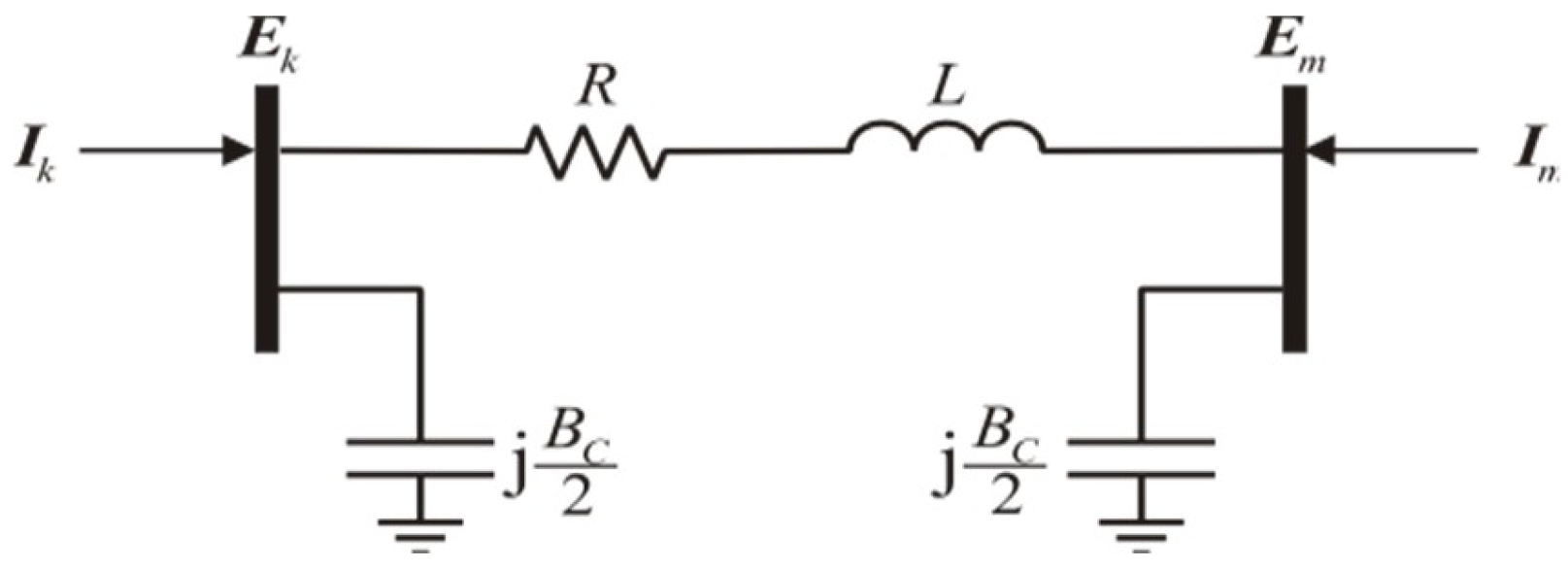
Each feeder is modeled as a line of transmission, as is illustrated in
Figure 1, where
Ii and
Ei are the phasors of the injected electricity and voltage, respectively, on the node
i (
i =
k,
m) of the microgrid.
R,
L, and
Bc represent the parameters of resistance series, inductance series, and shunt susceptance, respectively, of the feeder. The relationship electricity–voltage of the equivalent circuit is given by Equation (5) [
21]. Admittance matrix elements are evaluated in Equations (4) and (5).
Starting from
Figure 1 and Equation (3) it is possible to obtain expressions that model the injection of active and reactive power—Equations (6) and (7), respectively—on the node
i (
i =
k,
m) at each moment
tT ∈
z [
21] where
j =
k,
m, being
j ≠
i. The variables
and
(
n =
i,
j) represent the magnitude and the angle of the nodal voltage phasor
Ei:
The decision variables associated to these feeders correspond to the nodal voltages in its terminals ().
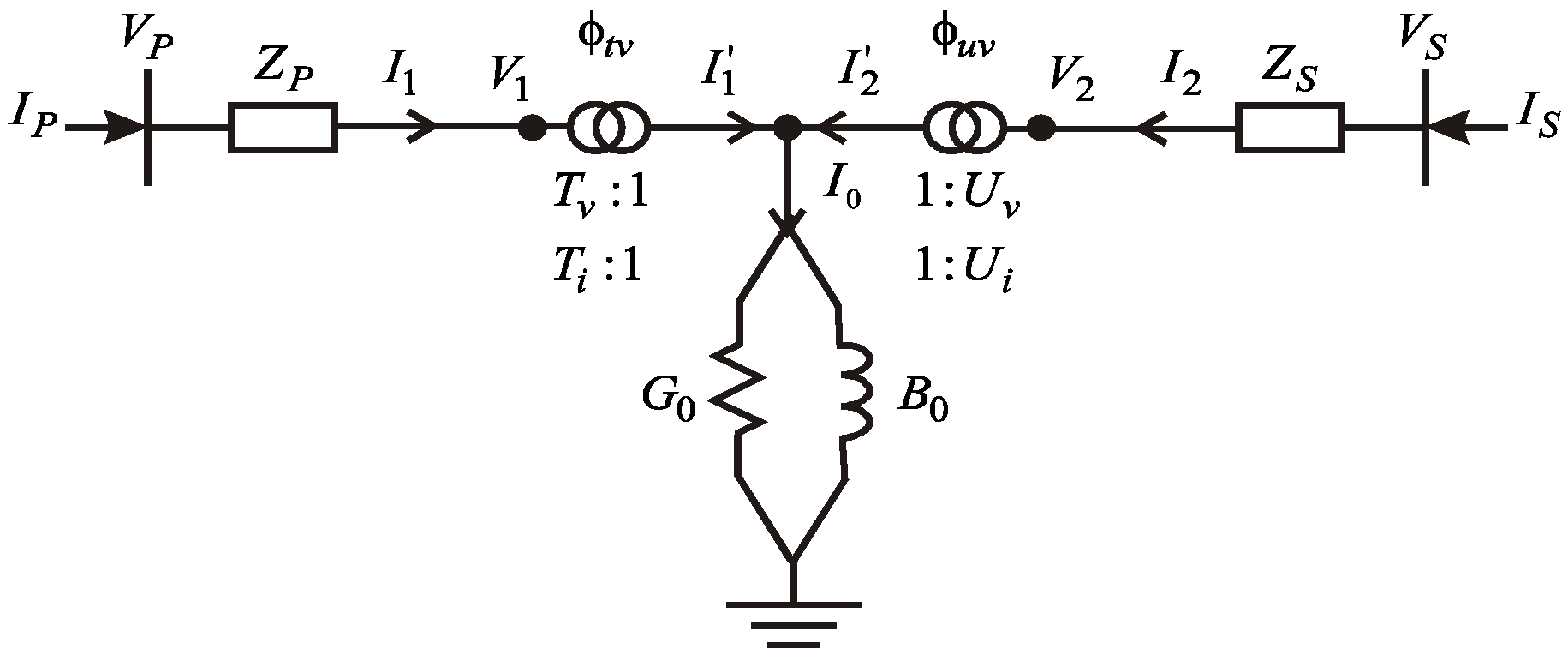
2.3. Transformer
The primary winding is considered an ideal transformer with relation to complex tap
Tv:1 and
Ti:1 in series with the impedance
Zp (refers to
Figure 2) where
Tv =
Ti* =
Tv∠
φtv, and the symbol * denotes a complex conjugate. The secondary winding is also represented as an ideal transformer with relation to complex tap
Uv:1 and
Ui:1 in series with the impedance
Zs where
Uv =
Ui* =
Uv∠
φuv. The relationship between voltage
Vp and electricity
Ip of the primary winding and the voltage
Vs and electricity
Is of the secondary one is given by Equation (8) [
21].
where
As the feeders, the injections of active and reactive power in the nodes of connection i and j, where i = p, s; j = p, s; i ≠ j are represented by Equations (6) and (7), but considering the conductance and susceptance matrices of Equation (8), it is important to highlight that the decision variables associated to transformers correspond to the nodal voltages in its terminals ().
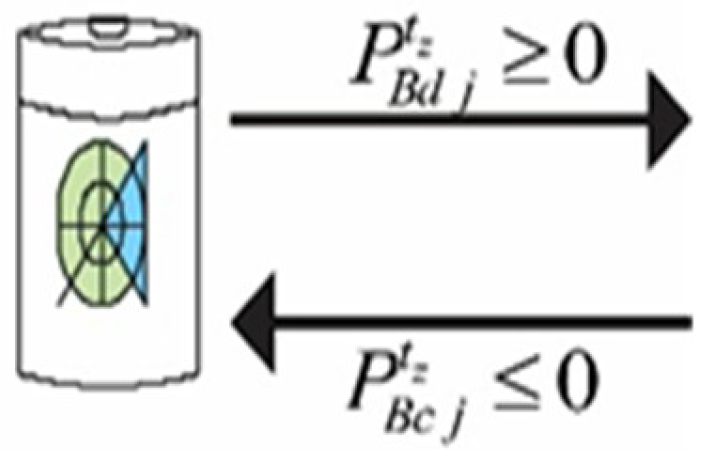
2.4. Batteries
The batteries are elements that can operate in charge or discharge mode to provide or consume a net amount of active power in their connection node. Then, the
jth battery is represented by two sources of active power, as shown in
Figure 3 [
22]. One of them represents the charge power
and the other the discharge power
; the sum of both powers represents the net power
provided or consumed by the battery in their connection node.
In addition, the voltage phasor in the connection node is represented by its magnitude
and its angle
. Thus, the decision variables of the
jth battery are
(
) where
are the battery variables, while
(
). Moreover, the State of Charge (SOC) of the
jth battery in the time
tz (
) can be approximated by means of Equation (10). In Equation (10),
represents the SOC at a given initial time
t0, whereas
Enom is the energy capacity of the battery, whose efficiencies for charge and discharge operations are given by
εcj and
εdj, respectively. Lastly, ∆
t is a fixed time step length.
It is assumed that the energy provided by the batteries has no cost since it is absorbed and provided in the same node of connection. However, since the optimization algorithm will manage the power, batteries will be charged in periods of low-cost energy and will be discharged in periods of high cost. This fact involves an economic benefit in the operation of the microgrid.
2.5. Wind Turbine
For the aim of the stationary analysis, the wind turbine can be considered a source of noncontrolled active power
, depending on its density
, wind speed
, and the area
covered by the blades of the wind turbine [
23].
Since it is considered that the power delivered by the wind turbine is not controllable, this element does not introduce decision variables. However, Equation (12) is required to assess the contribution of the power of the jth wind turbine for a wind speed curve, ; density, , and area, , given. Clearly, the magnitude and angle of the voltage phasor of the connection node are considered decision variables, such that (). Finally, it is assumed that the energy provided by the wind turbine has no cost. In addition, a good forecast for wind speed curves is considered to be available.
2.6. Photovoltaic Modules
Figure 4 shows the schematic model of a photovoltaic module connected to the
kth node through a DC/AC converter [
24]. The implicit expression showed in Equation (12) models the behavior of the DC current in
panel terminals, where
Iph,
I0,
,
Rs,
ns, and
np represent the current of the photovoltaic panel, the current of saturation, the DC voltage in the module terminals, the resistance in series, and the number of cells in series and in parallel, respectively. The term
Rs is evaluated from Equation (13), where
Voc,
Vmp,
I, and
Imp represent the open circuit voltage, the voltage of the point of maximum power, short circuit electricity, and maximum power point electricity, respectively. Terms
Isc and
Voc are evaluated through Equations (14) and (15), respectively, where
Isc,stc,
G,
Gstc,
ki,
T,
Tstc,
Voc,stc, and
kv represent the short circuit electricity standard under conditions of test, irradiance under test, electricity temperature coefficient, temperature of the panel, standard temperature under test, standard low open circuit voltage conditions test, and voltage and temperature coefficient, respectively.
In this work, the photovoltaic module parameters involved in Equations (12)–(15) were taken from the features of the polycrystalline module ATERSA A-222P [
25]. Moreover, a good forecast of solar irradiance curves is considered to be available.
According to the model in
Figure 4, the injected power in DC terminals (generated by module) can be expressed directly as
Moreover, the balance of power between the AC and DC terminals of the inverter must also be fulfilled. If the losses of the converter are rejected, then
where
is the active power injected at the terminals of the primary transformer coupling module;
and
are the magnitude and the angle, respectively, of the voltage phasor for such terminals; and
and
represent the same but for the secondary terminals. Therefore,
in Equation (17) is formulated explicitly by means of Equation (7), but considering the matrix of conductances and susceptances of Equation (9). It is important to mention that, due to being considered a DC/AC converter multipulse with 48 pulses, the following relationship must also hold [
26]:
It is important to highlight that the decision variables introduced by the photovoltaic module are (), whereas ().
2.7. Electrical Load
Energy consumption in load nodes of the microgrid is represented by a model of constant power for any interval of time
T. The
ith complex power
consumed in the node is then represented by Equation (19) where
and
represent the power consumption active on that node at the instant
tz.
The model of energy demand does not introduce decision variables to the optimization problem, but the magnitude and angle of the connection node phasor voltage must be considered decision variables, such as (). In addition, it is assumed that a good forecast of the energy demand curves is available ().
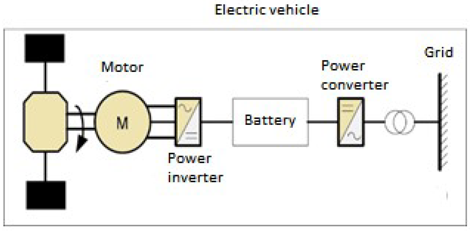
2.8. Electric Vehicle
Nowadays, tendencies exist to make energy consumption more efficient to satisfy transportation needs. In this case, it is necessary to consider that an Electric Vehicle (EV) will be connected into a microgrid to charge its battery efficiently. Also, the EV will work as a storage system responsible for energy management and optimization within the microgrid.
The structure of an EV is constituted mainly by an AC engine, a three-phase power rectifier (AC/DC), a storage system (battery), and a three-phase power inverter. This last component injects power from the storage system to the grid (
Figure 5). The three-phase power inverter is considered as a Controlled Voltage Source (CVS), which has the ability to control the active and reactive power flow between the EV and the microgrid [
27].
The real power and the reactive power injected are represented through the Equations (6) and (7), respectively. Supposing that power loss does not exist on the CVS, the power storage in the battery and the active power injected by the CVS are the same with an equality constraint, Equation (20).
The State of Charge (SOC) of an EV in a determined time is described by the Equation (21) [
28]. The energy consumption for an instant of time
t,
, is the result of the sum of the energy storage at time
t − 1,
, the energy consumed at time
t,
, and the sum of the energy charged
and the discharged energy
at time
t:
where
is the charge efficiency coefficient of EV,
the discharge efficiency coefficient of EV, and
the differential of operational time. It is necessary to consider that the charged power is negative
and the discharged power is positive
, where the sum of these powers represents the total power injected or consumed by the battery of the EV on the grid point.
In addition, the voltage phasor in the connection node is represented by a magnitude and an angle . Thus, the decision variables of the jth battery of the EV are () whereas ().
5. Results
Before discussing the numeric results related to the optimal energy management in microgrids through the optimal power flow (OPF) implemented in this work, it is necessary to describe the microgrid and the hardware used for the simulation of the OPF.
Firstly, the microgrid is called microgrid test (MT), and is composed of an integrated system of a photovoltaic panel (PV), a wind turbine (WT), a storage system (battery, BT), a main grid (MG), electric transformers (ET), a Park of EV (PEV), and a point of load within the system. The MT is selected as a case study to show the results of the optimal energy management obtained from the tools selected. Moreover, the generators in the microgrid use a real irradiance profile, wind speed profile of Almería city, and the electricity demand curve. All previous data were taken from Laboratory 6 of the CIESOL with different climatic variabilities.
Subsequently, an analysis of the computational performance of the interior point method (fmincon), hybrid genetic algorithm with interior point (GA-IP), and direct search hybrid with interior point (patternsearch-IP) is presented, which allows us to identify the most effective methods for solving the model presented in Equations (26)–(29). Finally, all the methods to solve the OPF are executed on a DELL computer, with 8 GB RAM and an Intel i5-4210U CPU@ 2.40 GHz processor (DELL, Mexico city, Mexico). The numerical results are reported in terms of per unit (PU) quantities.
5.1. CIESOL Building
In this paper, several optimization methods are compared at a time to optimize the economic energy dispatch within a microgrid. Besides this, with the aim to evaluate the performance of each optimization method with different scenarios, real climatological data of solar radiation, wind speed, photovoltaic system data, and laboratory load saved during regular operation of the CIESOL building (
http://www.ciesol.es) were considered. CIESOL is a solar energy research center placed inside the Campus of the University of Almería in the south-east of Spain; see
Figure 6.
More specifically, this building is divided into two different floors with a total surface approximately equal to 1072 m2. In addition, it has been designed to be a Nearly-Zero Energy Building (NZEB), and, thus, it has several bioclimatic criteria such as the use of photovoltaic panels to produce electricity and a Heating, Ventilation, and Air Conditioning system based on solar cooling which is composed of a solar collector field, a hot water storage system, a boiler, and an absorption machine with its refrigeration tower.
Furthermore, the CIESOL building works as a research center which deals with the study of the implemented bioclimatic strategies, the analysis of their influence over energy efficiency, and greenhouse-effect gasses reduction, and, also, the development of optimization techniques to increase the ratio of renewable energies use against conventional ones. For this reason, it uses a wide network of sensors and actuators whose measured data is stored in a database by means of measurement and acquisition software. More specifically, the building has a meteorological station composed of different types of sensors (e.g., temperature, relative humidity, direct and diffuse irradiance, CO2 concentration, etc.) and the building rooms measure air temperature, plane radiant temperature, globe temperature, relative humidity sensors, and power meters in order to measure the energy consumption in each room. In order to use a load profile to compare the different optimization methods, one of the representative rooms of the CIESOL building has been selected as a reference, specifically, Laboratory 6. This room was chosen among the characteristic ones mainly due to its occupancy profile. In more detail, this room works as an office and it is placed in the upper floor of the CIESOL building. In addition, it is characterized by having north orientation, a volume of 76.8 m3, and a window with a total surface of 2.15 × 2.09 m2.
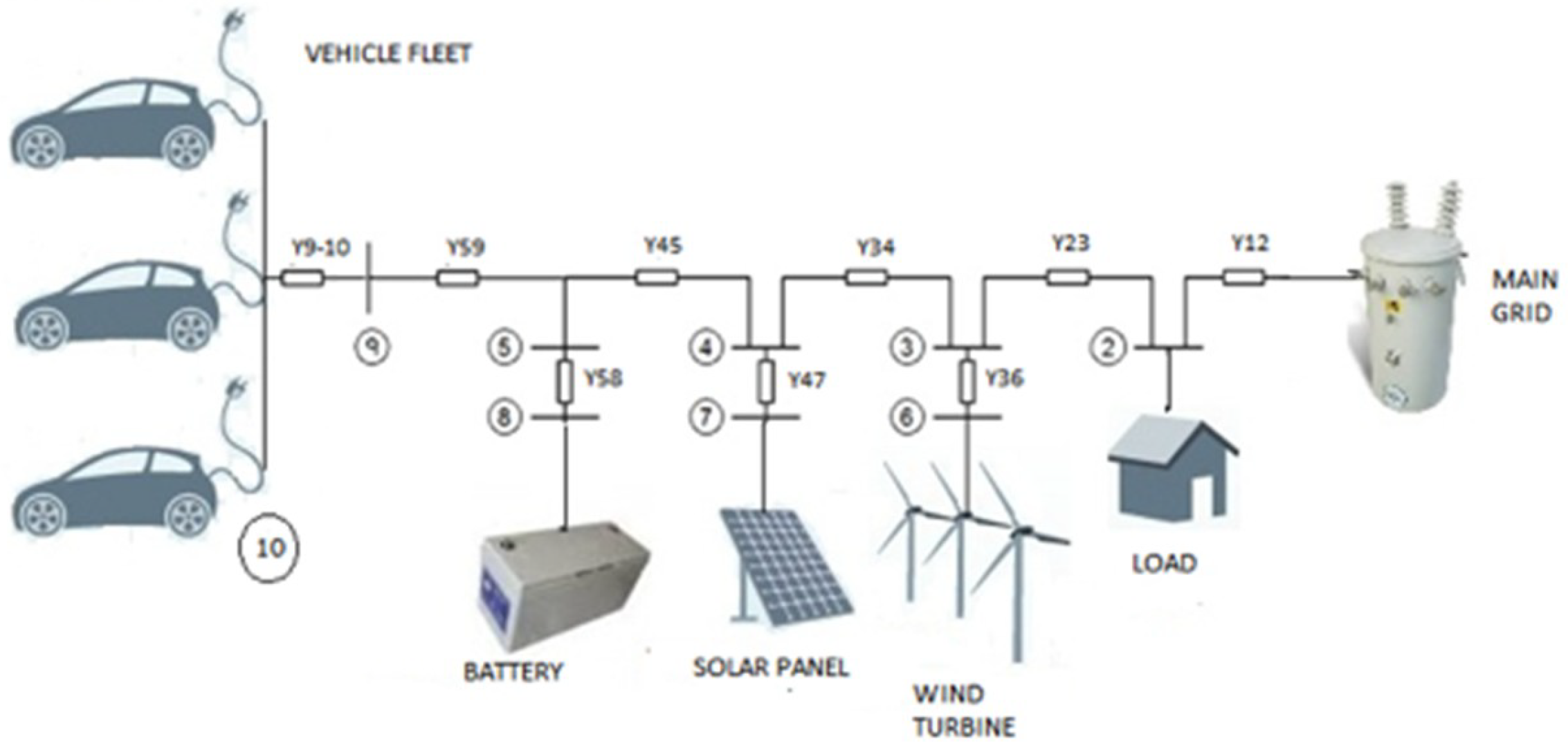
5.2. Microgrid Test
The microgrid test (MT) described previously is shown in
Figure 7. The microgrid is connected to the main grid through the single PCC (Node 1). Furthermore, between the Nodes 3–6, 4–7, 5–8, and Nodes 9, 10, there are transformers connected. The elements that have the ability to provide active power are the main grid (PCC), WT, PV, PEV, and the battery. The parameters considered for modeling the components of this MT and the cost coefficients associated with imported energy through the PCC are presented in
Table A1 and
Table A2 given in
Appendix A.
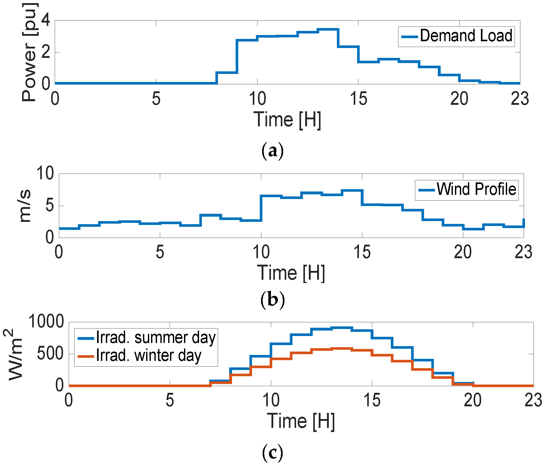
The PEV are composed of four EV, while the forecasting curve of load, the irradiation profile for two different clear days (summer and winter), and the speed of wind corresponding to the city of Almería, Spain, can be observed in
Figure 8. All the power within the microgrid is working on per unit (p.u.), where the power base and voltage base were selected to be 10 kW and 100 V, respectively.
The voltage magnitude limits for all nodes in the microgrid are
p.u. The SOC limits on the battery are
, whilst the initial condition of the battery charge is
. Moreover, all the cars in the PEV will be connected to the microgrid at hour 8 and disconnected at hour 18. All the cars have initial SOC as shown in
Table 1. To compensate the owners of the EV for the use of the battery, at the end of hour 18, the SOC in the battery will be 100% (SOCPVH
). The SOC limits in the PEV for all the EV are
.
The OPF was solved using the interior point method provided by the “fmincon” function developed by MATLAB®, the direct search method with interior point hybrid (GA-IP), and hybrid genetic algorithm with interior point (patternsearch-IP); their results are discussed below.
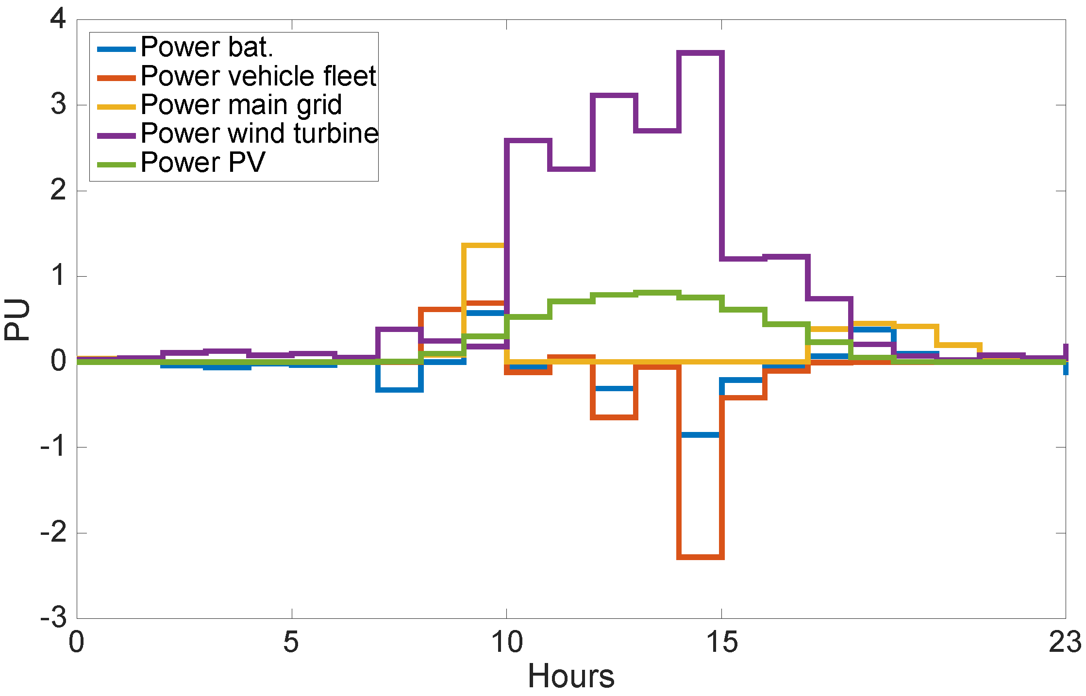
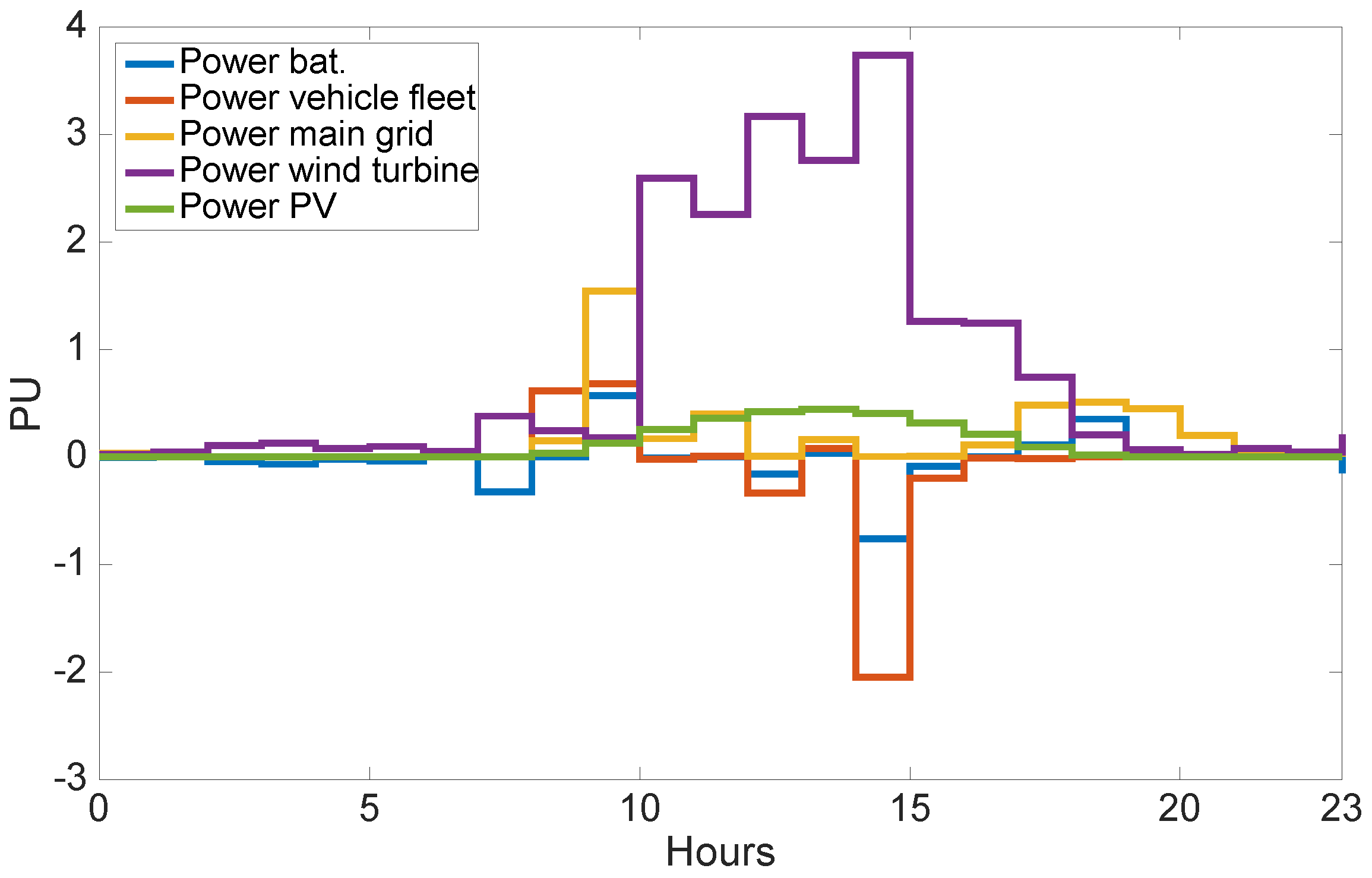
Figure 9 shows the active power supplied by the battery, PEV, WT, and PV, and the imported power from the main grid. The powers of the PV and WT are for a clear summer day. This figure shows that between the stages 0 and 6 h or 20 and 24 h the power demand by the load is small (35 kW), and the generators (PV, WT) and batteries supply this power to satisfy the load demand. Nevertheless, between 8 and 10 h or 16 and 20 h, the power supplied by the generators and the batteries is not enough to supply the load demand, making it necessary to import power from the main grid to satisfy the load and avoid problems within the microgrid. In addition, the PV have the maximum power supplied between 9 and 17 h, agreeing with the forecasting profile of irradiance shown in
Figure 8a; in the same way, the maximum power of WT corresponds to the maximum speed of wind predicted by the forecasting profile of wind speed shown in
Figure 8b.
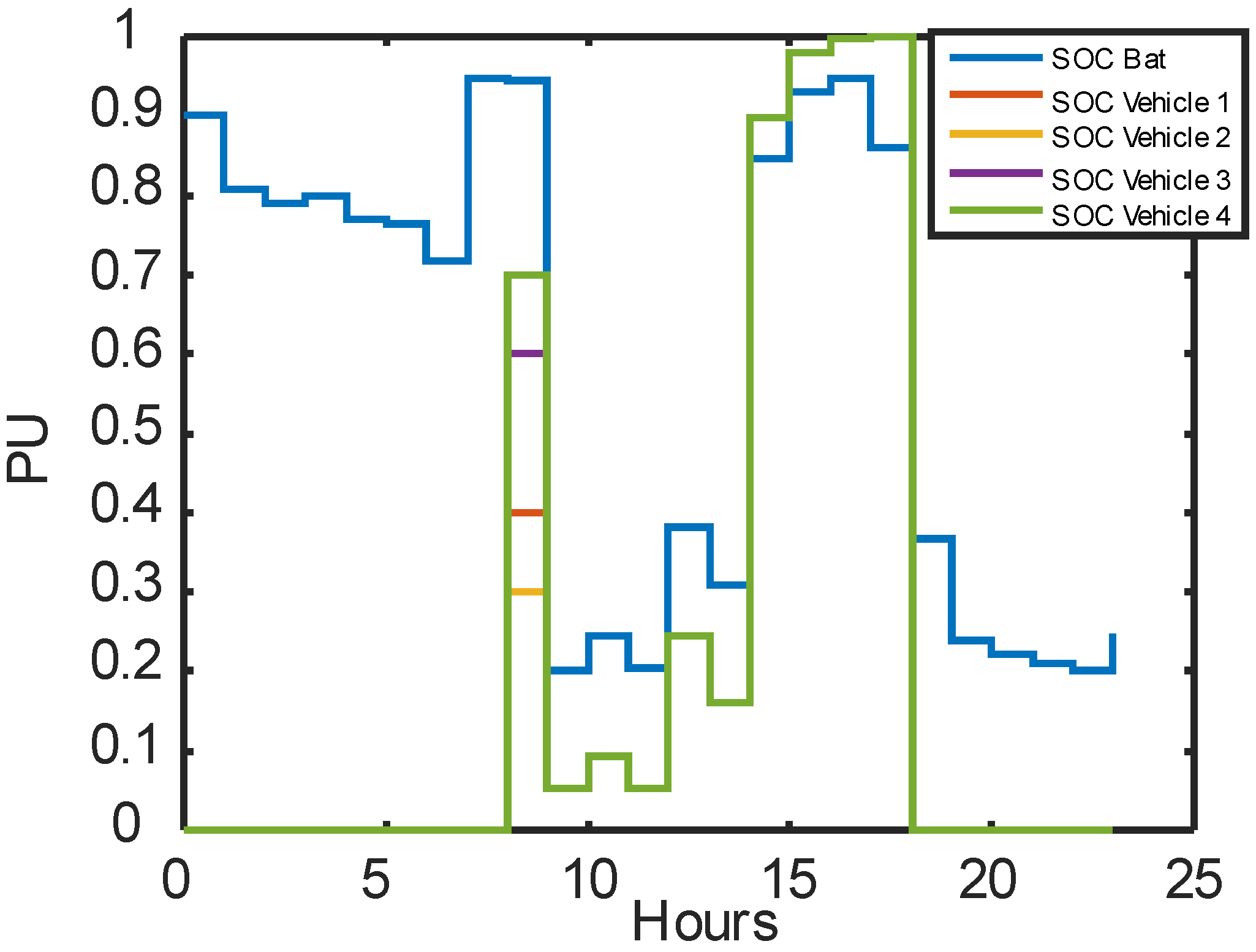
It is noteworthy that the PEV and the battery are working in charge mode when the power supplied by the PV and PW is high. This power storage in the PEV and battery is important to reduce the energy cost when peak load demand exists (8–10 h with PEV and 16–20 h with battery)—in other words, to reduce imported power from the main grid.
Figure 10 shows the state of charge of the battery and the PEV, confirming the previous idea.
In
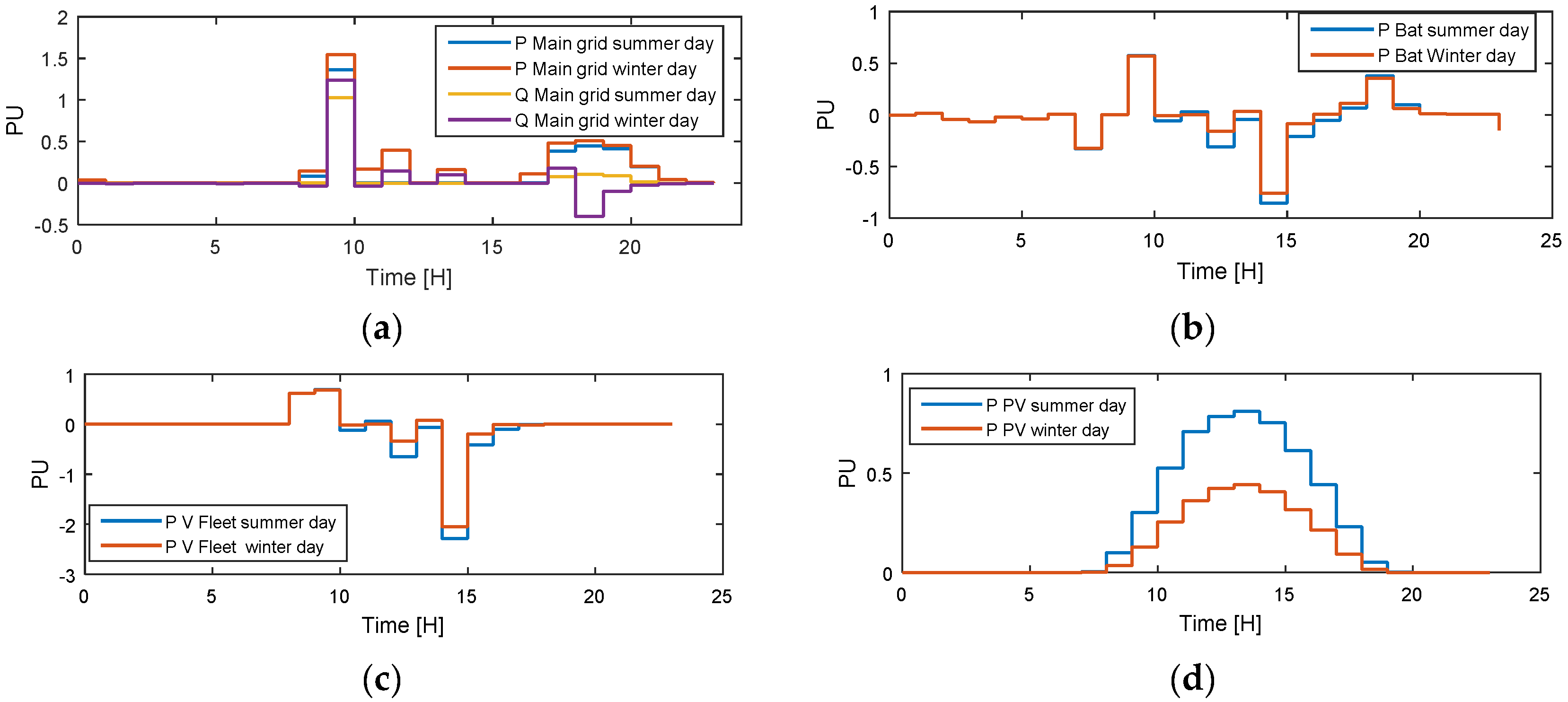
Figure 11 it is possible to see the active power supplied by the elements within the microgrid (WT, PV, Battery, PEV, and Main grid) on a clear winter day. It is important to understand that the power supplied by the PV on a clear winter day is less than on a clear summer day. This reduction of power produces an increment in the imported power from the main grid and a gradual decrement in the power supplied by the WT, battery, and the PEV. Those increments and decrements in the power flow inside the microgrid are shown in
Figure 12 through a comparison between the power generators on summer and winter days.
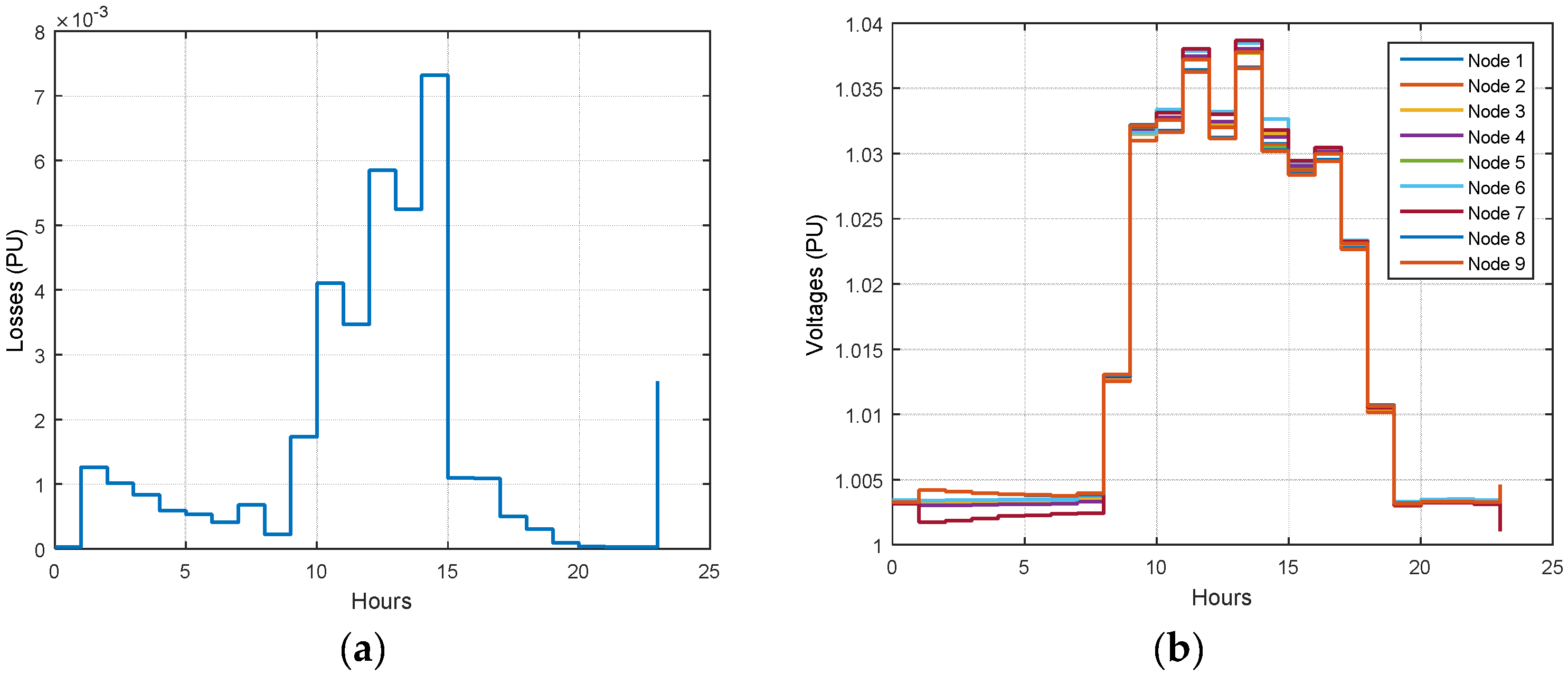
Figure 12 shows the active (P) and reactive (Q) power flow exchanged between the main grid and the microgrid through the PCC for the whole time period T of interest (24 h). Also, the active power provided by the electric vehicles, battery, and photovoltaic system is shown in that figure. It is observed that the amount of active and reactive power exchanged with the main grid through the PCC changes along the time period T. This is due to the optimal energy dispatch driven by the proposed approach, which handles the energy storage systems under the variation of the system load demand and the power generated by the renewable generation systems. This optimal energy management also involves low total active power losses and an acceptable voltage profile. For example, for the microgrid operating on a summer day,
Figure 13 shows the low total active power losses obtained along the time period T. This fact is expected in this approach because loss reduction involves a decrement in the power imported from the main grid and, hence, in the total cost, which aids to minimize the fitness function. Also, the bus voltage profiles satisfy the specified operating limits (0.95 ≤
V ≤ 1.05) for the whole time period
T, which is ensured in this approach because the bus voltage limits are explicitly considered in the proposed models (26)–(29).
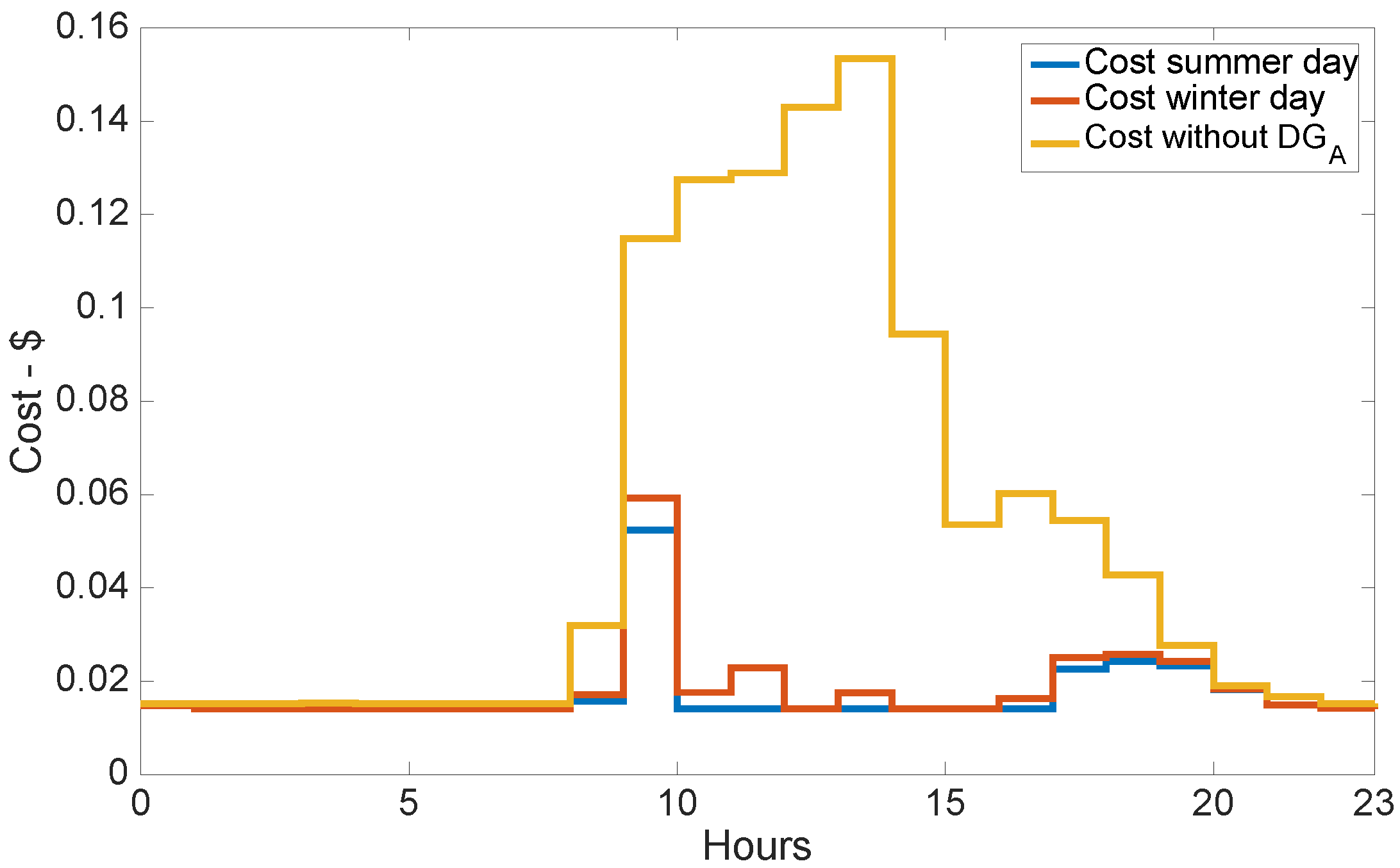
The total energy costs of the imported power from the main grid without DG and with DG during winter and summer days are shown in
Figure 14 When the microgrid is working without DG, high cost occurs when there is peak load demand. Nevertheless, the main aim of this paper is the optimization when the microgrid works with DG, and we observe in
Figure 13 that the aim is being met in full. However, differences exist between the energy cost when the microgrid operates on clear summer and winter days (energy cost is higher when it is a winter day). This is because the irradiation is lower on a winter day, generating less power compared to a sunny summer day, making the import of power more expensive from the main grid when it is a winter day.
5.3. Performance Comparison between Different Methods
This section presents the performance of the IP, GA-IP, and patternsearch-IP methods for solving the optimization problem given by the model in Equations (26)–(29). That performance is presented based on a comparison of the fitness value achieved at the optimal solution of Equations (26)–(29) and the CPU run time spent for three different microgrid setups. The microgrid under study is the one given in
Section 5.2. The first and second setups consider the irradiance profiles for a summer day and a winter one and assume that all components of the microgrid illustrated in
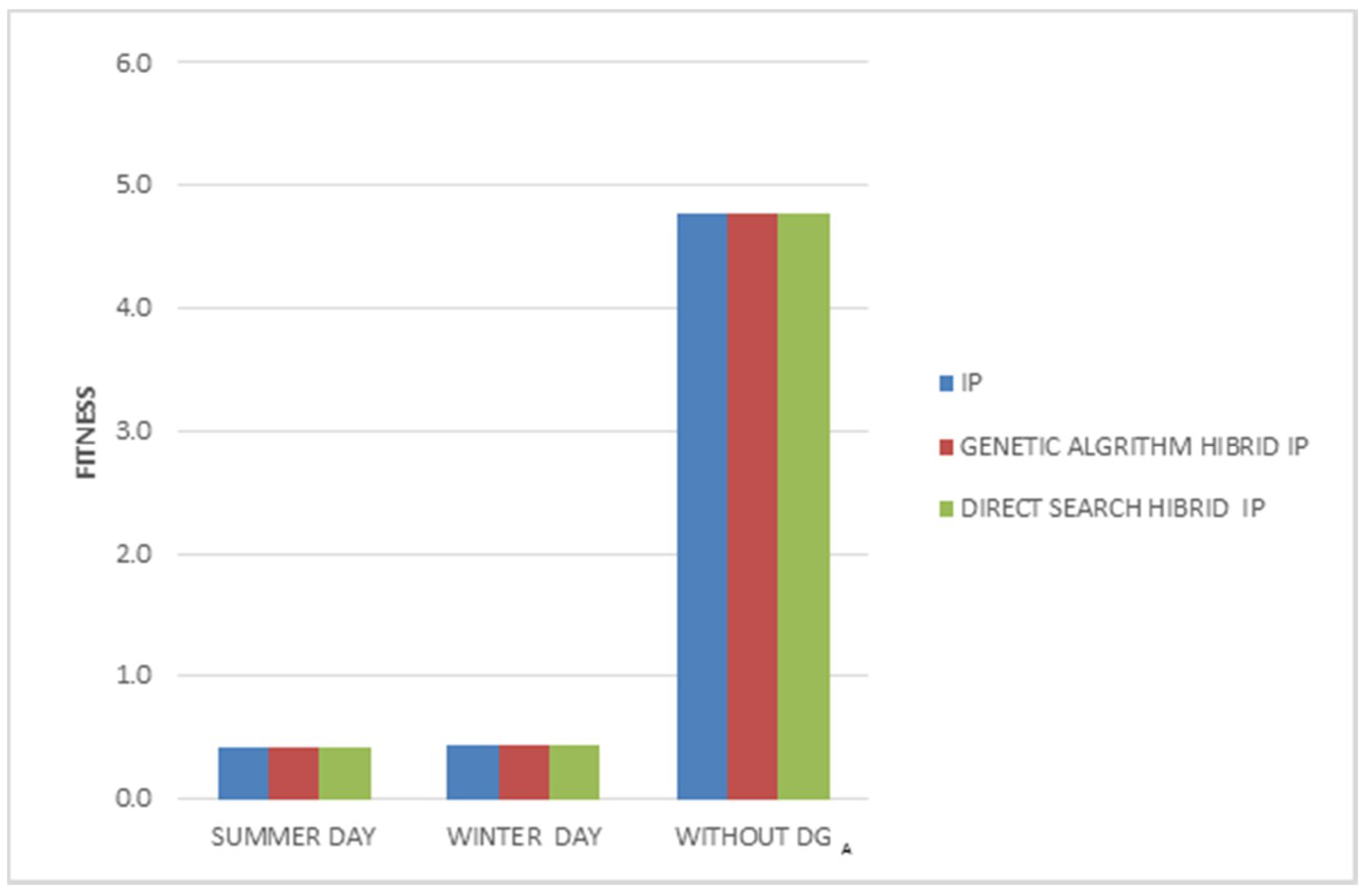
Figure 7 are online. The third setup considers the irradiance for a summer day, but assumes that the distributed generation (wind and PV) and storage (batteries and electric vehicles) systems of the microgrid are offline. The performance of the three suggested methods obtained for the three microgrid setups is as follows.
Figure 15 provides the value of the fitness Equation (26) achieved by the IP, GA-IP, and patternsearch-IP methods at the optimal solution of the optimization problem in Equations (26)–(29) for the three different microgrid setups. It is clearly observed that for each microgrid setup, the three methods have achieved practically the same value of the fitness function. These results suggest that they perform similarly in terms of effectiveness, i.e., they all obtain the same fitness function value when solving the optimization problem in Equations (26)–(29). On the contrary, their performance in terms of computing time is substantially different, as discussed below.
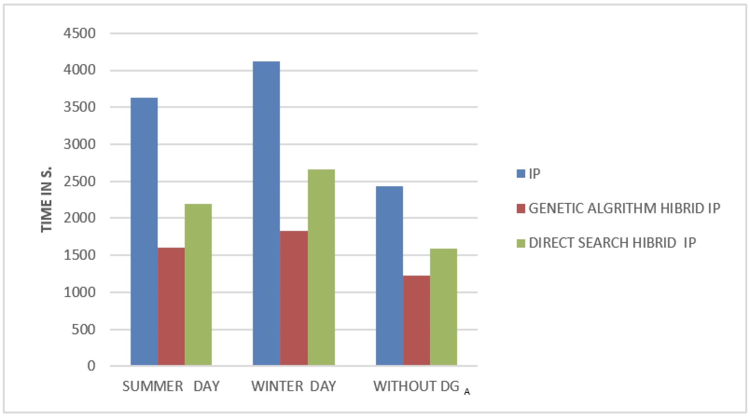
Figure 16 shows the CPU time spent by the IP, GA-IP, and patternsearch-IP methods for solving the optimization problem in Equations (26)–(29), for each one of the three different microgrid setups. As can be seen, GA-IP is the fastest algorithm for all the cases, followed by the patternsearch-IP algorithm. Please note that the GA-IP method is 57% (20%) faster than the IP method (patternsearch-IP method). Then, the results may suggest that hybrid algorithms are able to obtain solutions of the same quality as the ones provided by the IP method, but consuming less computing time.
However, it is important to point out that the CPU time spent by the hybrid algorithms may importantly depend on the optimization problem size. Then, bearing in mind the aforementioned, the size of the studied microgrid in this work, and the obtained results in this section, it must be concluded that the CPU time performance of hybrid methods shown here might be expected for small-scale microgrids.

 and
and 


