Drivers of Electricity Poverty in Spanish Dwellings: A Quantile Regression Approach


Department of Applied Economics (Econometrics), Universidad Autónoma de Madrid (UAM), 28049 Madrid, Spain
*
Author to whom correspondence should be addressed.
Energies 2019, 12(11), 2089; https://doi.org/10.3390/en12112089
Submission received: 29 April 2019
/
Revised: 23 May 2019
/
Accepted: 28 May 2019
/
Published: 31 May 2019
Abstract
:The main objective of this article is to explore the causes of household electricity poverty in Spain from an innovative perspective. Based on evidence of energy inequality across households with different income levels, a quantile regression approach was used to better capture the heterogeneity of determinants of energy poverty across different levels of electricity expenditure. The results illustrate some interesting and counter-intuitive findings about the relationship between household income and electricity poverty, and the technical efficiency of quantile regression compared to the imprecise results of a standard single coefficient/OLS approach.
1. Introduction
Energy poverty and vulnerability are critical issues. According to current research, the problem is extensive and even severe in many countries. Recent data available from the EU survey on Income and Living Conditions estimates that around 11% of the EU population were unable to keep their home adequately warm. In the particular case of Spain, where a long and serious economic crisis have greatly deteriorated living conditions for millions of people, some recent reports have warned about the extent of this problem [1], urging politicians and energy companies to take an active role in the debate.
The main objective of this article is to explore the causes of household electricity poverty in Spain, with a special focus on the impact of household income levels on electricity power expenditure.
Standard analyses of electricity consumption for a given country, region or area, frequently use average household expenditure ratios that do not fairly represent the whole population they attempt to describe. The average value of energy household spending is not of real interest if different levels of energy consumption are caused, affected or reversed by different factors with different intensity. In this context, electricity poverty, understood as an extreme value of energy relative expenditure, deserves particular attention. Lessons learnt from empirical studies that aimed to explain electricity household consumption as a whole, might not be extrapolated to the poorest households and are not of particular interest when it comes to determining how to tackle electricity poverty at the household level.
Although ordinary regression (OLS) has been the most used technique to estimate energy poverty drivers, nowadays, the availability of microdata allows more granular and accurate estimates of the effects of each of the explanatory variables within this phenomenon. The implicit simplification of the classical regression (focusing in the mean) can be useful for aggregate data but it can also obscure the very interesting nuances that we can discover using microdata. When exploring poverty drivers, it is crucial to focus on vulnerable populations, however, by using segmented samples and subsamples, the statistical results will be biased.
Additionally, the presence of heteroscedasticity and frequent outliers in microdata dramatically affects the OLS estimates. Conversely, quantile regression (based on absolute errors instead of square errors, and also using the total sample, but differently weighted by subsamples) produces consistent and efficient estimates even in data showing these potential problems.
Finally, it is worth mentioning that quantile regression can produce different coefficients for the same driver (explanatory variable) depending on the referred electricity poverty quantile. As we want to focus on a vulnerable population, it is not necessary to have a mean coefficient for the entire population, but rather, a very specific coefficient for the poorest population. OLS does not allow such a distinction and produces a mean coefficient. As we will show below, quantile regression is a useful tool for discovering the real effect of each one of the drivers on electricity poverty.
Consequently, quantile regression emerges as the most suitable technique to perform a fruitful analysis of the explanatory variables of electricity household relative expenditure. As will be shown later, estimated coefficients for the main drivers of electric energy household consumption present very different values across different energy relative expenditure quantiles.
The present paper clearly complements the existing literature in this field. Firstly, although there exists a vast amount of literature on the causes of average energy consumption using standard econometrics, a quantile approach is not that common. Additionally, even though the drivers of electricity consumption or saving have received extensive attention in the economic literature at a cross-country level, there are very few studies specifically related to electricity poverty (or vulnerability) in a developed context, and at the household level [2].
Specific attention to household behaviour and causes of electricity poverty for families is crucial from a policy perspective at a time when debates about different dimensions of economic and social exclusion have gained momentum in the political arena, even in the context of well-developed EU countries. In the age of new technologies and globalization of mass communication, electricity scarcity not only affects basic needs such as heating, food or sanitation, but also hinders access to communication, e-learning activities, e-commerce, etc.; electricity poverty emerges as a contemporary driver of social inequality.
Not all explanatory variables of energy poverty are available or accurately measured in the available statistics. In this article, we were able to find a wide set of variables referring to household equipment, the characteristics of the people who live there, socio-economic status, and even several behaviour-related variables (gender, studies, nationality, etc.). Unfortunately, many other variables such as physical characteristics of the building, available electrical appliances, and indoor-outdoor temperature difference were not available.
Certainly, this restriction limits the scope of the analysis, but conversely, several fundamental variables such as income, the way of heating the home, ownership characteristics, etc., have been shown to be useful for suggesting various political measures that could be promoted (see the Discussion section). In addition, the selected technique makes it possible to eliminate the inherent biases in the use of mean values, instead using those that are most appropriate for the vulnerable population.
This article is structured as follows. In Section 2, a review of the theoretical and literature background is carried out, highlighting the main variables and estimation techniques previously used in other texts. In Section 3, we summarise some of the advantages of the quantile regression approach in the context of electricity poverty analysis. In Section 4, a descriptive analysis of the data is conducted. In Section 5, the results of the quantile regression are discussed, and the main conclusions are outlined.
2. Definitions, Theoretical Background and Literature Review
2.1. Definition of Energy Poverty/Vulnerability
Day et al. [3] (p. 260) define “energy poverty” as “an inability to realise essential capabilities as a direct or indirect result of insufficient access to affordable, reliable and safe energy services, and taking into account available reasonable alternative means of realising these capabilities”. A similar characterisation is used in [4] (p. 31): “the inability to attain a socially and materially necessitated level of domestic energy services […] tied to the ineffective operation of the socio-technical pathways that allow for the fulfilment of household energy needs”. This broad definition can be applied to all socio-economic spectrum and is valid either for under-developed or well-developed countries; in the case of our study in Spain, “insufficient accessibility” should be understood not as a physical barrier, but as a budget constraint.
The term energy poverty is commonly associated with household energy deprivation and commonly used in this sense across EU countries where, in recent years, this problem has gained momentum as part of the political and social debate in the context of spreading inequality. The EU “Third Energy Package” [5] also uses the term in this sense.
In our paper, we focus our econometrical analysis on the specific concept of “electricity poverty” or “electricity vulnerability”. Electrical power can be considered the main and default source of energy in a household, and therefore, it is the component that best captures the condition of energy deprivation in a household. Also, we wanted to align our conclusions with public policy issues, and in that sense, electricity poverty has become the public policy standard measure in Spain when it comes to implementing aid programs for vulnerable families.
We should admit that the use of electricity poverty explicitly excludes household energy expenditure for the basic need of heating homes in winter. In order to avoid bias in our analysis, we will control for substitutive energy expenditures in the household given that, alternative sources of energy used extensively by families in Spain such as natural gas for heating or boilers, may have a clear impact on electricity expenditure. Including natural gas expenditure as a control variable is also essential in the case of Spain given that temperatures are quite heterogeneous, to the point that heater devices are almost never used during the whole year in parts of the country. The Household Budget Survey (HBS) for 2015 shows that more than 33% families do not have heating systems in their homes. The average percentage varies from 97% in Canary Islands, Ceuta or Melilla, to around 5% in central regions, or 50% in southern coastal areas.
The UK was a pioneer in addressing this problem, and from early 1996 established some mechanisms to help people expending more on household energy than a fixed percentage of their total incomes (10%). As pointed out in [3] (p. 256): “Annual ‘excess winter deaths’ statistics for the UK show every year a peak in the number of deaths during winter months that run to the tens of thousands […] a fact which is generally attributed to the poor energy efficiency of the UK housing stock, making houses expensive to heat”.
On the other hand, the use of electricity as the pivotal variable to identify energy vulnerability is especially suitable for Spain because of the widespread use of air conditioning during the hot Spanish summer. While some authors consider that issues related to cooling households are not essential and should not be included in the concept of “energy poverty”, other authors disagree (see [6], for example). The effects of extremely high temperature on labour conditions, health, and quality of life are obvious, and access to AC devices should be explicitly considered in terms of energy poverty.
In the case of France, which is maybe more similar to the Spanish case (where heating is not always the main problem), the definition of “energy precariousness” is “a person encountering ‘particular difficulties in their accommodation in accessing the necessary energy supply to satisfy basic needs, due to inadequacy of financial resources or of housing conditions” [7] (p. 8).
As a final caveat, it is worth mentioning that measures of energy vulnerability or scarcity are commonly addressed by computing energy consumption, but we need to realize that people do not directly demand energy itself, but the services provided by electricity or other sources. Families demand energy for washing, cooking, lighting, HVAC, mobility, etc. Therefore, some authors have proposed a different focus called a services approach, where the level of satisfaction with these services determine the definition of electricity poverty. Essentially, this is similar to measuring income poverty by looking at material deprivation or affordability of some items thought to be indispensable for people to have a satisfactory standard of living. Unfortunately, it is almost impossible to get detailed household data about energy services available in households.
2.2. Measuring Electricity Poverty: the Income Effect
There is no unique, consensual definition of how to identify households in energy poverty, but using the idea of high spending/low-income, many authors, European countries’ experts, and the EC itself [8], continue to use the ratio of household expenditure on energy as an unbiased description of energy poverty. For the particular case of electricity, a simple way of estimating the energy vulnerability of a family is to examine the ratio between average per capita energy expenditure over family income.
By computing the decile thresholds for this ratio at the national level, we can then identify an “at risk of energy poverty household” when the ratio for that household is above the 80% or 90% decile threshold (or another similar arbitrary limit such as two times the national median).
Income dynamics and energy expenditure may follow different dynamics and be reactive to different policy measures [9], but the aim of this relative measure is to relate energy poverty with income poverty; the ratio may worsen if income conditions deteriorate, and/or energy expenditure increases (due to changes in prices, temperature or living conditions).
This type of ratio has been criticized because families facing income restrictions may adjust their energy expenditure, especially for heating their homes in winter, to under the optimum level [10]. Even if this is true for some countries and for some types of energy expenditure, the Spanish data for electricity expenditure do not confirm this idea. Data shown in the table below illustrate that except for the poorest households (There is another exemption for the highest revenue group but this could be considered atypical or anecdotical because only 55 observations (out of a total of 21,735 households) were included in this sample group.), total electricity expenditure is quite inelastic to household income levels, which supports the use of this standard ratio as our variable of analysis. In effect, per capita electricity demand is around 369 euros for almost all of the revenue levels (see Table 1).
The reason for this inelasticity in the Spanish case could be that electricity is used for heating only in a small number of dwellings, as most are located in warm locations. Services provided by electricity expenditure are so essential (lighting and plug-in devices such as fridge, washing machine, and ceramic hobs) that electrical bills becomes quite difficult to adjust below a certain minimum level. If this hypothesis is true, we can then assume that an increase in family revenue will not automatically produce an increase in the electricity bill (except for poorest households) but a change in the electricity poverty ratio. It should be remembered, that the relationship between income and energy poverty is central in our article: we do not only want to determine the main causes of electricity poverty but to explore the differential effects of the factors across different income levels.
2.3. Drivers of Household Electricity Poverty
Household energy poverty usually occurs because of a triad of high-energy prices, low income and poor energy efficiency in the residence (see Figure 1).
Different variables for these three different areas and intersections are commonly used in the literature. Following this approach, we also use a four group classification of explanatory variables that could be related to electricity consumption (see Table 2).
In a recent study, Middlemiss and Gillard [2] carried out an interview among “vulnerable families” in the UK. Based on their qualitative assessment, they found six categories of variables that were significantly related to vulnerability: quality of dwelling fabric, energy costs and supply issues, stability of household income, tenancy relations, social relations within the household and outside, and ill health. The main contribution of this paper is their findings in regard to the private and public efficiency of the strategies to cope with vulnerability.
Most of the variables included in the previous table have a clear connection with electricity consumption.
Geographical context is normally a clear determinant of electricity consumption. In the case of Spain, there are regional disparities in climate conditions, but considering that electricity is not commonly used for heating (only around 14% of dwellings according to the Families Budget Survey, 2018), the impact of regional climate may not be very relevant. Nevertheless, regional average electricity consumption shows large heterogeneity across Spain (see Table 3 below) suggesting the need to add a regional dummy indicator as a control variable. This variable would account for other climate conditions such as sunlight hours, and at the same time, would control for other sources of unobserved regional heterogeneity that may bias the rest of the coefficients.
The variables related to dwelling characteristics and household equipment are of great importance but, unfortunately, for most of countries, it is very difficult or impossible to gather homogeneous micro data at a national level. In the Spanish case, we do not have this type of data, but at least for those households who spend on electricity we were able to examine the Household Budget Survey (HBS). Our proposal is, at least, to control for building age (disposable at the level of the household data) as a proxy of several variables related to dwelling infrastructure. We expect that an older dwelling will be associated with higher electricity consumption because of poorer energy efficiency [12,13]. For the size and type of electrical appliances, family income will probably work as a proxy variable.
In the category of family status, household size and family composition are often identified as very important variables to define energy demand [14,15]. Some authors have also highlighted the indeterminate effect of tenure in dwelling consumption. Sardianou [16] and Vaage [14] found that owners tend to consume more energy than tenants. Conversely, Rehdanz [17] and Meier and Rehdanz [18] found negative or no significant effect.
In the group including usage/behavioural variables, some characteristics related to educational skills, gender, nationality and household age structure are encompassed. Using similar sets of variables, Ping Du et al. [19] and Belaid and Garcia [20] emphasized the crucial role of personal behaviour in final electricity consumption. Based on previous findings [21], the authors verified that household energy consumption can vary up to three times because of behavioural patterns, even when the buildings share similar characteristics.
Regarding electricity price, 95% of consumers pay the so-called “last resource tariff” in Spain so, in our view, it is not crucial to have a measure of prices using a cross section analysis.
3. Methodology
There is a vast amount of literature on estimating electricity consumption or saving behaviour at the dwelling level, but it is not so common to find specific studies about electricity poverty or electricity vulnerability.
The technical or statistical approaches used to analyse energy or electricity consumption drivers are very heterogeneous [22]. Swan and Urgusal [23] propose a simple classification of different techniques depending on the initial approach defined by researchers: top-bottom or bottom-up. In both cases, time series analysis of electricity demand is more frequently used than cross-sectional data analysis.
From a top-down point of view, a macroeconomic approach rules the individual’s typical consumption behaviour. For the bottom-up approach, available temporal and cross-sectional microdata allow more or less accurate predictions of short-term future consumption by family units. Focusing on the latter, because it is the approach selected in this paper, authors frequently distinguish between statistical and engineering techniques. In the first case, they highlight regression, conditional demand analysis, and neural networks as the preferred methods to estimate the relationship among selected explanatory variables and electricity demand. In the second case, population distribution, archetype and sampling methods are the most common techniques.
In a recent article, Fumo and Biswas [24] suggest that the use of traditional regression analysis in this area of research has become quite common in recent years due to the availability of more micro residential data on energy habits and consumption. Technological advances, for accurate measurements of electricity consumption per hour, partially explain the re-adoption of regression to understand family patterns of spending. Even by using such a simple model, we get reasonable accuracy in short-term forecasting.
Although traditional regression has been the preferred technique to estimate electricity demand, some authors have pointed out the difficulties of this analytical tool in capturing the marginal effects at the individual level. The huge and very informative heterogeneity observed in micro data is somewhat ignored when using traditional regression because it mainly focuses on the average behaviour [25].
Additionally, a rigid standard regression would normally fail in the presence of heterocesdasticity, frequent outliers, non-normality, non-linearity, and/or non-permanent coefficients for each explanatory variable, depending on the relative level of the final electricity consumption.
As is well known, the basic linear regression model rests on the assumptions of Gauss-Markov compliance to ensure that the obtained estimators are linear, unbiased, optimal and consistent. These imposes several conditions on the model: the hypotheses of linearity in the mathematical relations; null mean, homoscedasticity and non-autocorrelation in the perturbations; and strict exogeneity (random perturbations will not be conditioned by the values of the explanatory variables). Additionally, the maximum likelihood estimator (GLS) will coincide with the Ordinary Least Square (OLS) estimator only if the random perturbations are distributed as normal, with zero mean and constant variance.
The proposed framework for making estimates using OLS in the regression to the usual mean is frequently violated. Maintaining equal response proportions of the explained variable to changes in the explanatory variable (linearity) does not always seem congruent. In this research, it seems reasonable to suppose, for example, that the response on electricity consumption for a very high-income situation cannot be the same as for a very low income. The economic effort involved in the first deciles of consumption for a low-income earner is surely much greater than that in the case of a high-income earner. In other words, covering a minimum electricity cost for those with low incomes will require a great deal of effort, while it will be practically irrelevant for those with high incomes.
Second, the hypothesis of homoscedasticity (variance of constant random disturbance throughout the sample) is also frequently violated in our case. It seems plausible that the determinants not expressly included among the explanatory variables, and, then, included in the random disturbance, will be very different if we consider low consumption levels rather than high level consumers.
Third, the hypothesis of normality of resids is violated both empirically (when regressions of cases such as the present are made using ordinary least squares) and theoretically. Again, it is difficult to think of homogeneous behaviour in a highly scalable consumption variable when dealing with low- and high-level consumers. Maintaining the mean as the most probable value is not data driven.
Quantile regression effectively deals with the previously defined limitations by relaxing the assumption of normality, although, essentially, it provides a different estimate of the coefficients for the different quantiles considered for the variable under study. In our context, this procedure makes sense if we suspect that the importance of the explanatory variables for electricity consumption is not homogeneous for the different levels of consumption. Thus, quantile regression emerges as the most appropriate technique to provide an accurate and impartial estimate of the effect of explanatory variables for the most vulnerable households.
As an alternative to the common OLS estimator based on the mean, the quantile regression estimator is based on the same idea, but it takes into account the median (or another selected quantile) and minimizes the sum of absolute resids (instead of the sum of square resids).
As Koenker and Basset [26] demonstrated, in the above equation, the equal weight of both the left and right sides of the endogenous variable produces an accurate estimate of the median. Therefore, by weighting each tail of the distribution by the desired quantile and minimizing the previous function, we can find the specific coefficients for any other quantum (call it τ%):
where the weighted factor (:
In the traditional regression for the mean, the estimated value of the endogenous variables corresponds to the mean hope conditioned by the set of variables and the explanatory parameters-variables Xβ, resulting in:
Similarly, we can write this expression for quantiles in the following way:
Therefore, we can estimate the coefficients for each quantum using the following expression:
This expression could be rewritten as follows:
where it is easy to observe the process underlying the quantile estimation method. Specifically, it would be a weighted estimation by using linear optimization algorithms, in which the observations included in the quantile of interest are more weighted than those outside the quantile. Seen differently, this procedure assigns a different weight for positive and negative errors, allowing the estimation of different parameters for each selected quantile.
To a certain extent, the use of absolute values versus the square of traditional regression minimizes the effect of outliers on the parameters estimated by treating them linearly and not “exaggerating” them through the square power involved in the OLS estimation.
Another additional advantage of this estimation method is that it allows us to avoid the so-called “Heckman selection bias” [27] present in many investigations that make multiple estimates using ordinary least squares and plotting the sample by deciles. This sample trimming produces biased parameters, and invalidates their later applicability. In the quantile regression, the total sample is always used, although conveniently weighted.
Although Koenker and Bassett [26] formulated quantile regression in the late 1970s, this technique has not been used often until recent times. In the past, two issues inhibited its feasibility: the complex minimization algorithm to obtain the coefficients, and the weakness of the confidence intervals of the estimated coefficients in the absence of the assumption of normality in random disturbances. Currently, the exponential growth in computational capacity and the ease of avoiding confidence interval problems through the use of bootstrapping techniques have produced an excellent scenario for using this technique without any difficulties (Several authors have addressed the problem of estimating the coefficients confidence intervals in the framework of this “semi-parametric” regression. Hoenker and Hallock [28] proposed up to five different alternatives for what are known as range inversion intervals. Powell’s estimator [29], known as the “Sandwich method”, determines the covariance of the estimators based on independent and identically distributed errors through sample randomization or bootstraping versions, obtaining results similar to those obtained previously by Hoenker and Hallock. Through various Monte Carlo experiments, Buchinsky [30] demonstrates that, in the face of heterocedasticity problems, the method of estimation using randomized sub-samples for the calculation of confidence intervals is the most robust).
4. Data
We used the annual Household Budget Survey published by the National Institute of Statistics (INE) for 2015 (the latest available). The HBS is identical across EU countries so that they can all be integrated later in a common Eurostat operation.
We decided to focus our analysis on the family level so we merged individual micro data sets with family’ data sets. The total number of observations in each wave is composed of nearly 21,500 dwellings.
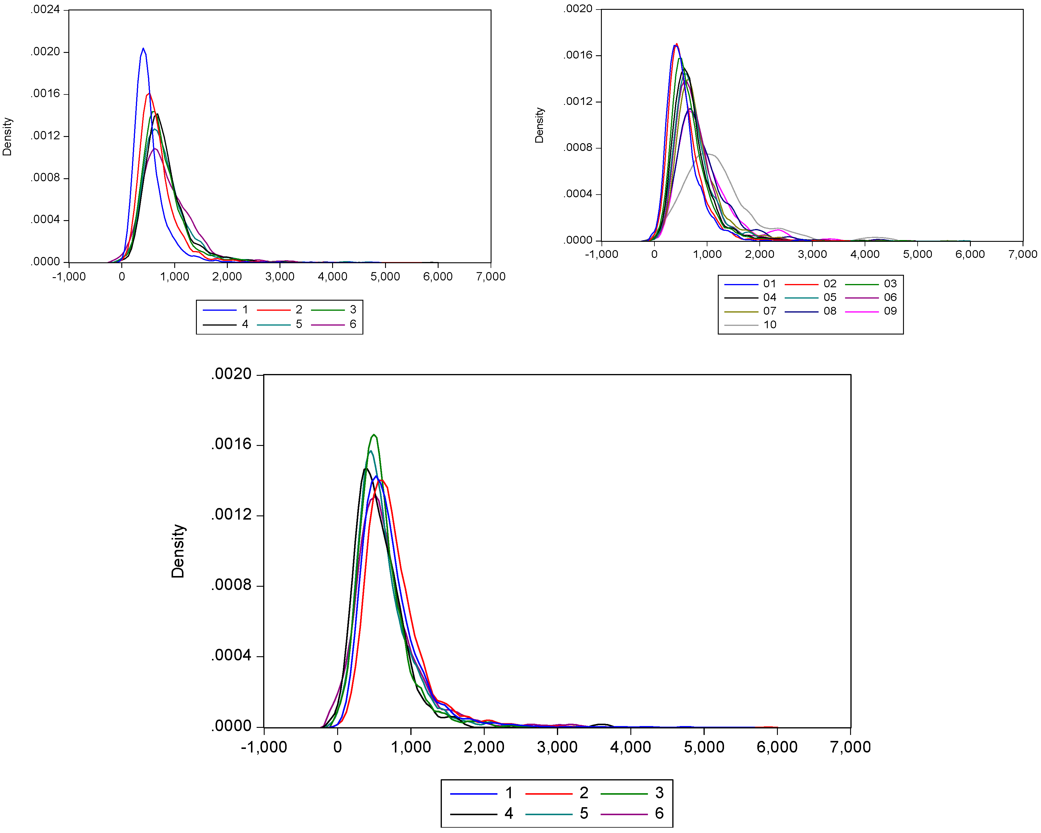
The endogenous variable (percentage of electricity expenditure over total revenues) clearly exhibits a non-normal distribution, and the mean and median are fairly distant as a result of a large number of outliers and extreme values. The standard regression on the average appears to be an inappropriate instrument when the mean is clearly a poor representation of the sample (see Figure 2). Additionally, bivariate graphs illustrate that, at the bivariate level, the relationship between electricity expenditure and potential explanatory variables is not constant across quantiles for our endogenous variables.
In the survey, the family most frequently includes has 2, 3 or 4 members (32%, 23% and 21% respectively). Families with just one member represent around 18% of the sample. Families of six members represent only 6% of the sample. Literature (and logic) indicate that a larger size of household is related to greater expenditure, but the increase in such expenditure is not proportional to the increase in the number of members. This heterogeneity in the effect of family membership on electricity consumption supports the thesis about the behavioural concerns cited above.
5. Results and Discussion
Not surprisingly, family income emerged as the most relevant variable in this study. The higher the income, the lower the probability of falling into electrical poverty (the coefficients indicate a reduction of this indicator as income increases). All income cuts are significant in both OLS and quantile regressions. Comparing OLS coefficients with the median coefficients (q = 0.5) easily shows the importance of outliers in defining a biased estimate if OLS parameters are used. As expected, the estimated quantile coefficients for these variables show an increase in the importance of reducing electrical poverty when considering higher values of this indicator: people in the highest part of the distribution of electrical poverty suffer a greater reduction of this situation when considering higher incomes. Non-linearity is fully confirmed by the evolution of these coefficients, and the use of OLS estimators produces a systematic bias and is affected by a problem of heteroscedasticity, so employing the quantile regression methodology proposed here is crucial.
The use of these estimates opens the door to more accurate policies that are focused directly on direct income support rather than on price reduction. Revenue policies could be graduated to the desired level taking into account the differences in parameters. The same level of reduction need not necessarily be applied for any given income, but can be done in tranches using the same coefficients shown here. Such policies could be applied through personal income tax deductions. If price reduction is the policy measure adopted (as in the recent Spanish Law), it should be assumed that the effect so far estimated would be significantly lower than the real effect because the OLS coefficients have been used. For lower incomes, the reduction by 7.8 percentage points in the electrical poverty indicator marked by the OLS coefficients underestimates the effect of the measure on the population most relevant to it, where said effect is greater than 10 points (80% quantile) or 12 points in the case of the poorest (90% quantile). Therefore, the measure is fully justified and its impact is almost double that estimated when OLS is used (see Table 4).
As noted above, the regional effect is extremely relevant in the characterization of electric poverty in Spain. All regions show a parameter significantly different from zero when quantile regression is carried out for the poorest deciles, which does not occur using the OLS model. All the autonomous communities have lower levels of electrical poverty with respect to the community taken as a reference: Andalusia. It is true that this difference is not very important considering the value of the coefficients, but if using the values estimated by OLS we observe differences of between 0.11 to 0.8 percentage points (of lower electrical poverty), while using the coefficients of the quantile regression we observe values closer to 1 point of difference in most regions.
Unfortunately, as already mentioned in previous sections, the results for the region variable are, by nature, imprecise, because the variable probably contains several other factors. In any case, the inclusion of the rest of the available control variables (such as income, population density, surface area and ownership of the dwelling, etc.) will probably isolate the climate factor in this variable, which we understood to be fundamental in our previous explanations (in both extreme cold and heat conditions). Note that the reference region, Andalusia, is the one that suffers the worst extreme heat conditions for a large number of months per year. Considering these differences, we may have a new mechanism to refine the implementation of the policy for reducing energy poverty which also takes into account the geographical nature of the recipients.
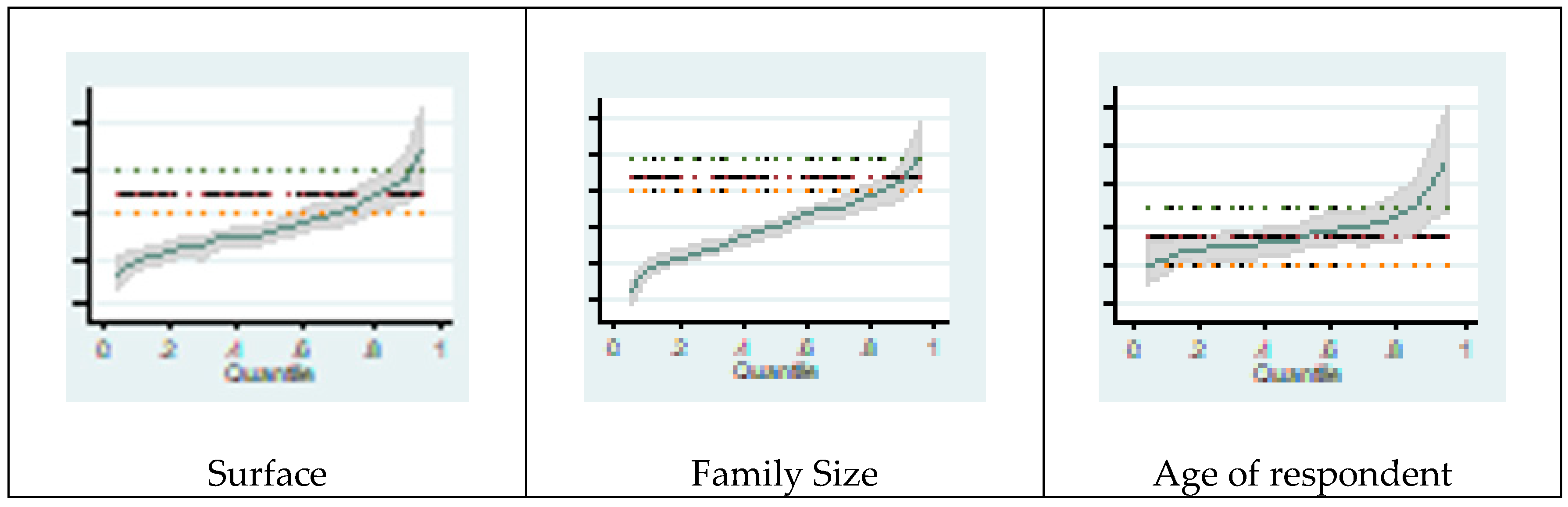
These graphs (see Figure 3) are useful to highlight once again the important bias that occurs when observing the parameters usually used (OLS) when the interest is focused on a very specific section of the sample (in our case, the higher quantiles, as the poorest households in terms of electricity, see Figure 3). The rest of the graphs can be seen in the Appendix A.
As expected, the type of fuel used to heat the home and/or water in the home is relevant. One point of reduction in poverty is shown when fuels other than electricity are used. It should be borne in mind that, as a basic control variable, the variable “gas-related energy poverty” has been included separately, in such a way that these coefficients would reflect how using fuels other than electricity sharply reduces poverty (almost two points in the poorest households observing the quantile coefficients). This observation leads to the need to leverage investment in more efficient and cheaper heating systems, such as gas versus electricity to reduce the electricity poverty gap.
As is well known, the fight against climate change promotes reduction in the use of gas by favouring greater electricity consumption. In view of our results, a difficult balance is established between not disadvantaging the most vulnerable dwellings in terms of electrical poverty and not harming the environment by favouring the consumption of gas for heating the home. Taking into account the accelerated learning curve in the use of clean energies, electricity generation could be carried out with lower production costs in the near future and, therefore, with lower prices, eliminating the current advantage of gas over electricity.
We briefly consider some of the other coefficients. For example, while the housing ownership regime is not significant in the OLS estimation, it is significant in the quantile regressions, where families with rented housing see their poverty gap slightly reduced when compared to the other tenure situations. Perhaps this is related to the excessive stock of owned dwellings in Spain, where typically families have large mortgages with little capacity to change their payment instalments during periods of crisis, a differential in families with rented housing, who can probably partially readapt their housing expenditure during these periods.
With regard to the characteristics of the parameters estimated for different educational levels, it should be noted that these levels are significant for the richest or middle class deciles (from 20% to 50%), but not for the poorest deciles (80% and 90%). This fact would not have been observed if only the results of OLS (where none of the levels are significant) were considered. It is also interesting to note that the parameters (around 0.35 points of greatest poverty before any educational level compared to the reference, those without formal education) are always positive and not different among the educational levels.
In short, all of these variables are useful points of information that can help to structure energy poverty policies in a more granular and successful way. The effect of policies, such as subsidies to change the heating system or income tax reductions for households with property debts should only be targeted at lower-income households if the aim is to reduce electricity poverty. Measures aimed at reducing consumption (as part of reducing the climate change impact of the use of this source of electricity) should clearly focus on changing the heat source.
6. Conclusions
In this article, the crucial issue of electricity poverty in developed countries has been characterised using the Spanish situation in 2016 as a case study. Although the study of energy poverty has been a common topic in the economic literature, it has usually focused on less developed countries. Because of emergence of inequalities and interest in climate issues in developed countries, research on this topic is now gaining momentum.
Traditionally, electricity demand, and to some extent, poverty research has been conducted using regression models based on the method of estimating least squares coefficients. Both because the focus of poverty is concentrated on very specific distribution quantiles and because the impact of some explanatory variables can change drastically if the distribution of the variable is considered, the findings of this article are especially important when considering alternative policy measures to avoid electrical poverty.
For example, as we have noted above, the findings of this investigation opens the door to more accurate policies that focus directly on direct income support rather than on price reduction. Revenue policies could be graduated to the desired level by taking into account differences in parameters. The same level of reduction need not necessarily be applied for any given income, but could be done in tranches using the same coefficients shown here. Such policies could be applied through personal income tax deductions. If price reduction is the policy measure adopted (as in the recent Spanish Law), it should be assumed that the effect so far estimated could be significantly lower than the real effect because OLS coefficients have been used. For lower income earners, the reduction by 7.8 percentage points in the electrical poverty indicator marked by the OLS coefficients underestimates the effect of the measure on the population that is most relevant, where said effect is greater than 10 points (80% quantile) or 12 points in the case of the poorest (90% quantile). Therefore, the measure used in this study is fully justified and its impact is almost double that estimated when OLSs are used.
In this article, we have shown the crucial differences in estimating the drivers of electricity poverty using OLS and using quantile regressors. Clearly, the use of the former produces a distorted picture of the reality, and results in a poor interpretation of the potential effects of public or private initiatives to reduce poverty.
Predictably, our research shows that income is the most important variable in relation to electrical poverty, but other variables such as the characteristics of housing tenure, or regional differences are also crucial when interpreting the effect of different anti-poverty policies.
Author Contributions
Both authors have contributed equally in all phases of this research, although Professor Mahía has focused more on the conceptualisation of the problem of energy poverty and Professor de Arce on its quantification and empirical analysis.
Funding
This research received no external funding.
Conflicts of Interest
The authors declare no conflict of interest.
Appendix A

Table A1.
Descriptive statistics of the explanatory variables.
| 2016 | 2012 | ||||
|---|---|---|---|---|---|
| Group | Variable | Mean | Std. Dev. | Mean | Std. Dev. |
| Region | Aragón | 0.044674 | 0.206593 | 0.044344 | 0.205863 |
| Asturias | 0.040442 | 0.196997 | 0.038621 | 0.192694 | |
| Balears | 0.034645 | 0.182882 | 0.036992 | 0.188747 | |
| Canarias | 0.04472 | 0.206694 | 0.045135 | 0.207605 | |
| Cantabria | 0.034553 | 0.182648 | 0.03555 | 0.185169 | |
| Castilla y León | 0.067219 | 0.250406 | 0.066307 | 0.248823 | |
| Castilla la Mancha | 0.055533 | 0.229022 | 0.055512 | 0.228981 | |
| Cataluña | 0.091511 | 0.288342 | 0.089247 | 0.285106 | |
| Valencia | 0.077755 | 0.267791 | 0.079289 | 0.270196 | |
| Extremadura | 0.045503 | 0.208409 | 0.045461 | 0.208318 | |
| Galicia | 0.06087 | 0.239096 | 0.060816 | 0.238998 | |
| Madrid | 0.07458 | 0.262719 | 0.072216 | 0.258852 | |
| Murcia | 0.040856 | 0.197961 | 0.041413 | 0.199247 | |
| Navarra | 0.033724 | 0.180523 | 0.035224 | 0.18435 | |
| País Vasco | 0.101035 | 0.301382 | 0.097855 | 0.297125 | |
| Rioja | 0.033126 | 0.17897 | 0.033595 | 0.18019 | |
| Ceuta | 0.005245 | 0.072234 | 0.005351 | 0.072957 | |
| Melilla | 0.005567 | 0.074406 | 0.005863 | 0.076347 | |
| Pop 50 k–990 k | 0.123948 | 0.329529 | 0.117584 | 0.322123 | |
| Pop 20 k–49 k | 0.152749 | 0.359754 | 0.150342 | 0.357415 | |
| Pop 10 k–20 k | 0.104072 | 0.305361 | 0.10865 | 0.311207 | |
| Pop < 10 k | 0.243892 | 0.429438 | 0.244242 | 0.429647 | |
| Intermediate density | 0.236531 | 0.424962 | 0.23461 | 0.423765 | |
| Low density | 0.288567 | 0.453106 | 0.293146 | 0.455215 | |
| Paired chalet | 0.24472 | 0.429931 | 0.251733 | 0.434019 | |
| Condo < 10 apartments | 0.177088 | 0.381752 | 0.180587 | 0.384685 | |
| Condo > 10 apartments | 0.470899 | 0.499164 | 0.460472 | 0.498447 | |
| Other | 0.001288 | 0.03587 | 0.001163 | 0.034088 | |
| Dwelling age | More than 25 years | 0.652404 | 0.476218 | 0.63045 | 0.482694 |
| Surface | 101.1462 | 49.61235 | 101.6724 | 49.6414 | |
| Water | Electricity | 0.229998 | 0.420841 | 0.217114 | 0.412291 |
| Gas | 0.394801 | 0.488819 | 0.374064 | 0.483891 | |
| Liquid gas | 0.238417 | 0.426125 | 0.27351 | 0.445771 | |
| Other liquid sources | 0.117598 | 0.322139 | 0.120748 | 0.325842 | |
| Solid sources | 0.005659 | 0.075015 | 0.005444 | 0.073585 | |
| Solar energy | 0.010674 | 0.102765 | 0.007073 | 0.083804 | |
| Not available | 0.000046 | 0.006783 | 0.0000465 | 0.006821 | |
| Heater | Electricity | 0.140189 | 0.347191 | 0.138849 | 0.345797 |
| Gas | 0.332505 | 0.471122 | 0.309851 | 0.462443 | |
| Liquid gas | 0.025673 | 0.158161 | 0.028384 | 0.166071 | |
| Other liquid sources | 0.142397 | 0.349465 | 0.149598 | 0.356685 | |
| Solid sources | 0.02259 | 0.148597 | 0.017403 | 0.130769 | |
| Solar energy | 0.00161 | 0.040097 | 0.000791 | 0.028115 | |
| Not available | 0 | 0 | 0.0000931 | 0.009647 | |
| Income | 500–1000 euros | 0.171659 | 0.377092 | 0.172305 | 0.377654 |
| 1001–1500 euros | 0.207177 | 0.405293 | 0.203806 | 0.402836 | |
| 1500–2000 euros | 0.167472 | 0.373405 | 0.171839 | 0.37725 | |
| 2000–2500 euros | 0.139821 | 0.346809 | 0.137267 | 0.344137 | |
| 2500–3000 euros | 0.10789 | 0.310249 | 0.114234 | 0.318102 | |
| 3000–5000 euros | 0.131125 | 0.337545 | 0.131171 | 0.337595 | |
| 5000–7000 euros | 0.021624 | 0.145456 | 0.021125 | 0.143805 | |
| 7000–9000 euros | 0.006257 | 0.078856 | 0.003583 | 0.059751 | |
| >9000 euros | 0.00253 | 0.050241 | 0.001582 | 0.039745 | |
| House tenure | Property with debt | 0.302001 | 0.459136 | 0.320087 | 0.466521 |
| Rented | 0.117184 | 0.321647 | 0.10772 | 0.310033 | |
| Rented (low payment) | 0.01095 | 0.104071 | 0.012936 | 0.113 | |
| Semi-free cession | 0.027421 | 0.163311 | 0.027919 | 0.164744 | |
| Free cession | 0.019462 | 0.138144 | 0.018426 | 0.13449 | |
| Nationality | Rest EU | 0.021256 | 0.14424 | 0.023638 | 0.151921 |
| Rest Europe | 0.003221 | 0.05666 | 0.002978 | 0.054491 | |
| Rest of the world | 0.054566 | 0.227137 | 0.053325 | 0.224685 | |
| Employment | Unemployed | 0.434967 | 0.495764 | 0.439719 | 0.496364 |
| Size | Household size (OECD) | 1.770412 | 0.547907 | 1.806831 | 0.557249 |
| Age | Age main income contributor | 55.6213 | 14.93647 | 54.29091 | 15.30132 |
Source: Family Budget Survey 2012 and 2016 (INE) and own calculations.
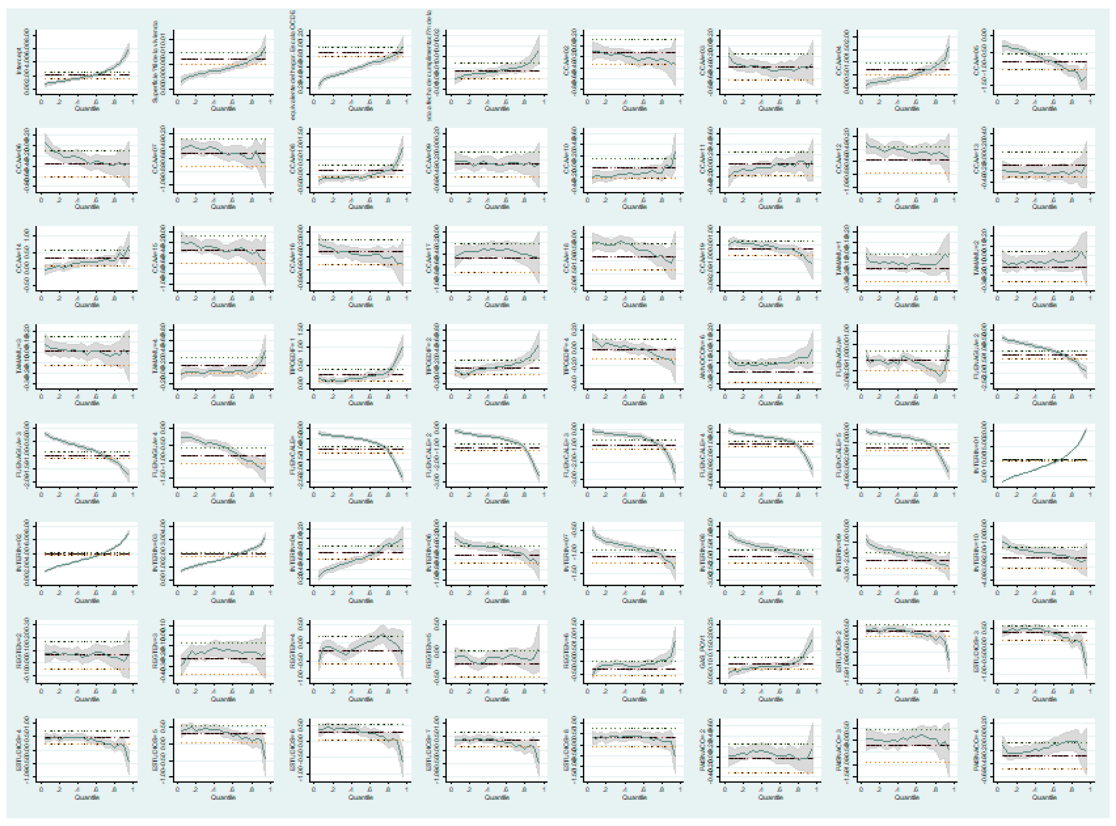
Figure A1.
Electricity poverty. Quantile coefficients.

References
- Tirado Herrero, S.; Jiménez Meneses, L.; López Fernández, J.L.; Perero Van Hove, E.; Irigoyen Hidalgo, V.M.; Savary, P. Pobreza Vulnerabilidad y Desigualdad Energética. Nuevos Enfoques de Análisis. Asociación de Ciencias Ambientales, 2018. Available online: www.cienciasambientales.org.es (accessed on 15 January 2018).
- Middlemiss, L.; Ross Gillard, R. Fuel poverty from the bottom-up: Characterising household energy vulnerability through the lived experience of the fuel poor. Energy Res. Soc. Sci. 2015, 6, 146–154. [Google Scholar] [CrossRef] [Green Version]
- Day, R.; Walker, G.; Simcock, N. Conceptualising energy use and energy poverty using a capabilities framework. Energy Policy 2016, 93, 255–264. [Google Scholar] [CrossRef]
- Bouzarovski, S.; Petrova, S. A global perspective on domestic energy deprivation: Overcoming the energy poverty–fuel poverty binary. Energy Res. Soc. Sci. 2015, 10, 31–40. [Google Scholar] [CrossRef]
- European Commission (EC). Third Energy Package; EC: Brussels, Belgium, July 2009. [Google Scholar]
- Harrison, C.; Popke, J. Because you got to have heat: The networked assemblage of energy poverty in eastern North Carolina. Ann. Assoc. Am. Geogr. 2011, 101, 949–961. [Google Scholar] [CrossRef]
- De Quero, A.; Lapostolet, B. Plan Batiment Grenelle, Groupe De Travail Précarité Énergétique Rapport. 2009. Available online: http://www.ladocumentationfrancaise.fr/var/storage/rapports-publics/104000012.pdf (accessed on 24 January 2018).
- European Commission (EC). An Energy Policy for Customers; Commission Staff Working Paper 2010; EC: Brussels, Belgium, 11 November 2010. [Google Scholar]
- Phimister, E.C.; Vera-Toscano, E.; Roberts, D.J. The dynamics of energy poverty: Evidence from Spain. Econ. Energy Environ. Policy 2015, 4, 153–166. [Google Scholar] [CrossRef]
- Brunner, K.M.; Spitzer, M.; Christanell, A. Experiencing fuel poverty. Coping strategies of low income households in Vienna/Austria. Energy Policy 2012, 49, 53–59. [Google Scholar] [CrossRef]
- Pye, S.; Dobbins, A. Energy Poverty and Vulnerable Consumers in the Energy Sector Across the EU: Analysis of Policies and Measures; Policy Report 2; INSIGHT_E: Brussels, Belgium, May 2015. [Google Scholar]
- Rehdanz, K. Determinants of residential space heating expenditures in Germany. Energy Econ. 2007, 29, 167–182. [Google Scholar] [CrossRef]
- Vaage, K. Heating technology and energy use: A discrete/continuous choice approach to Norwegian household energy demand. Energy Econ. 2000, 22, 649–666. [Google Scholar] [CrossRef]
- Estiri, H. Building and household X-factors and energy consumption at the residential sector: A structural equation analysis of the effects of household and building characteristics on the annual energy consumption of US residential buildings. Energy Econ. 2014, 43, 178–184. [Google Scholar] [CrossRef]
- Kelly, S. Do homes that are more energy efficient consume less energy? A structural equation model of the English residential sector. Energy 2011, 36, 5610–5620. [Google Scholar] [CrossRef]
- Sardianou, A. Estimating space heating determinants: An analysis of Greek households. Energy Build 2008, 40, 1084–1093. [Google Scholar] [CrossRef]
- Petrick, S.; Rehdanz, K.; Wagner, U.J. Energy use patterns in German industry: Evidence from plant-level data. Jahrbucher Fur Nationalokonomie Und Statistik 2011, 231, 379–414. [Google Scholar]
- Meier, H.; Rehdanz, K. Determinants of residential space heating expenditures in Great Britain. Energy Econ. 2010, 32, 949–959. [Google Scholar] [CrossRef] [Green Version]
- Du, P.; Zheng, L.Q.; Xie, B.C.; Mahalingam, A. Barriers to the adoption of energy-saving technologies in the building sector: A survey study of Jing-jin-tang, China. Energy Policy 2014, 75, 206–216. [Google Scholar] [CrossRef]
- Belaid, F.; Garcia, T. Understanding the spectrum of residential energy-saving behaviours: French evidence using disaggregated data. GATE Lyon Saint-Etienne WP 1536—December 2015. Available online: ftp://ftp.gate.cnrs.fr/RePEc/2015/1536.pdf (accessed on 24 January 2018).
- Summerfield, A.J.; Pathan, A.; Lowe, R.J.; Oreszczyn, T. Changes in energy demand from low-energy homes. Build. Res. Inf. 2010, 38, 42–49. [Google Scholar] [CrossRef]
- Yue, T.; Long, R.; Chen, H. Factors influencing energy-saving behaviour of urban households in Jiangsu province. Energy Policy 2013, 62, 665–675. [Google Scholar] [CrossRef]
- Swan, L.G.; Ugursal, V.I. Modeling of end-use energy consumption in the residential sector: A review of modeling techniques. Renew. Sustain. Energy Rev. 2009, 13, 819–1835. [Google Scholar] [CrossRef]
- Fumo, N.; Biswas, M.R. Regression analysis for prediction of residential energy consumption. Renew. Sustain. Energy Rev. 2015, 47, 332–343. [Google Scholar] [CrossRef]
- Kaza, N. Understanding the spectrum of residential energy consumption: A quantile regressión approach. Energy Policy 2010, 38, 6574–6585. [Google Scholar] [CrossRef]
- Koenker, R.; Bassett, G. Regression quantiles. Econometrica 1978, 46, 33–50. [Google Scholar] [CrossRef]
- Heckmann, J.J. The common structure of statistical models of truncation sample selection and limited dependent variables and a sample. Ann. Econ. Soc. Meas. 1976, 5, 475–492. [Google Scholar]
- Koenker, R.; Hallock, K.F. Quantile regression. J. Econ. Perspect. 2001, 15, 143–156. [Google Scholar] [CrossRef]
- Powell, J.L. Handbook of Econometrics; Engle, R., MacFadden, D.L., Eds.; Elsevier Science, B.V.: Princeton, NJ, USA, 1994. [Google Scholar]
- Buchinsky, M. Estimating the asymptotic covariance matrix for quantile regression models: A Monte Carlo Study. J. Econ. 1995, 68, 303–338. [Google Scholar] [CrossRef]
Figure 1.
Energy poverty triad. Source: Pye et al. [11].
Figure 1.
Energy poverty triad. Source: Pye et al. [11].

Figure 2.
Electricity expenditure by household size (up-left), by family income (up-right) and by tenure regime (down). (The total electricity expenditure has been trunked to lower than 7000 to enhance the visualisation of the graph). Source: Own elaboration Kernel density using Family Budget Survey, 2016 (INE).

Figure 3.
Electricity poverty. Some quantile coefficients.

Table 1.
Per capita yearly electricity expenditure. By monthly revenue level.
| Monthly Revenue | Mean | Median | Std. Dev. | Obs. |
|---|---|---|---|---|
| <500 euros | 344.2473 | 294.5735 | 222.4565 | 966 |
| 500–1000 euros | 391.3066 | 340.3448 | 256.0153 | 3731 |
| 1001–1500 euros | 375.3440 | 322.9200 | 253.1211 | 4503 |
| 1500–2000 euros | 370.9687 | 317.6848 | 243.9479 | 3640 |
| 2000–2500 euros | 363.8701 | 311.5983 | 228.3826 | 3039 |
| 2500–3000 euros | 352.2644 | 306.3529 | 237.3860 | 2345 |
| 3000–5000 euros | 350.2464 | 300.0000 | 222.2108 | 2850 |
| 5000–7000 euros | 363.5584 | 313.6333 | 233.3433 | 470 |
| 7000–9000 euros | 378.5435 | 326.0500 | 209.2936 | 136 |
| >9000 euros | 588.7737 | 375.0000 | 676.7883 | 55 |
| GLOBAL | 368.8893 | 316.6667 | 243.7883 | 21,735 |
Source: Own calculations with 2015 data from Household Budget Survey (National Institute of Statistics-INE). OECD house size equivalence was taken to estimate the per capita expenditure.
Table 2.
Classification of variables driving electricity poverty.
| Environment/Geographical Variables | Neighbourhood Density Heating and Cooling Degree-Days Climate Urban Structure |
|---|---|
| Usage/Behavioural variables | Gender Nationality Professional occupation Educational skills Household size and family age structure |
| Dwelling/Infrastructural variables | Geometry, envelope fabric Equipment and appliances Indoor temperatures Heating system Equipment use Building age |
| Family status | Ownership status (tenure) Housing type Family income Occupancy schedules |
Table 3.
Regional electricity consumption per dwelling (MW).
| Mean | Percentile 25 | Median | Percentile 75 | Interquantile % of Difference (Difference between the 75% and 25% Percentiles Divided by the Median) | |
|---|---|---|---|---|---|
| Andalucía | 715 | 420 | 623 | 894 | 76.0% |
| Aragón | 668 | 399 | 570 | 789 | 68.5% |
| Asturias | 584 | 344 | 491 | 709 | 74.4% |
| Baleares | 865 | 480 | 736 | 1100 | 84.1% |
| Canarias | 584 | 336 | 509 | 720 | 75.5% |
| Cantabria | 598 | 360 | 518 | 727 | 70.8% |
| Castilla y León | 576 | 340 | 493 | 708 | 74.6% |
| Castilla–La Mancha | 755 | 404 | 606 | 900 | 81.7% |
| Cataluña | 659 | 366 | 544 | 816 | 82.8% |
| Valencia | 701 | 406 | 600 | 882 | 79.4% |
| Extremadura | 681 | 371 | 577 | 840 | 81.4% |
| Galicia | 630 | 360 | 537 | 791 | 80.2% |
| Madrid | 653 | 384 | 557 | 804 | 75.4% |
| Murcia | 752 | 420 | 660 | 960 | 81.8% |
| Navarra | 581 | 365 | 512 | 720 | 69.3% |
| País Vasco | 583 | 355 | 500 | 720 | 72.9% |
| La Rioja | 552 | 354 | 490 | 692 | 69.0% |
| Ceuta | 452 | 282 | 408 | 581 | 73.2% |
| Melilla | 660 | 420 | 600 | 780 | 60.0% |
Source: Own Elaboration from Household Budget Survey 2012 and 2016 (INE) and own calculations.
Table 4.
Regression results for Indicator 1 of electricity poverty. (Endogenous variable: Electricity Expenditure/Total Expenditures) × 100.
Table 4.
Regression results for Indicator 1 of electricity poverty. (Endogenous variable: Electricity Expenditure/Total Expenditures) × 100.
| Reference | Variable | OLS | 0.2 | 0.3 | 0.5 | 0.8 | 0.9 | ||||||
|---|---|---|---|---|---|---|---|---|---|---|---|---|---|
| Intercept | 2.133 | *** | 1.288 | *** | 1.497 | *** | 1.932 | *** | 3.408 | *** | 4.670 | *** | |
| Surface | 0.005 | *** | 0.003 | *** | 0.003 | *** | 0.004 | *** | 0.005 | *** | 0.007 | *** | |
| Family Size | 0.753 | *** | 0.419 | *** | 0.472 | *** | 0.584 | *** | 0.750 | *** | 0.839 | *** | |
| Resp. Age | 0.004 | *** | 0.001 | * | 0.002 | ** | 0.003 | *** | 0.006 | *** | 0.009 | *** | |
| Gas Pov. | 0.098 | *** | 0.082 | *** | 0.086 | *** | 0.095 | *** | 0.111 | *** | 0.142 | *** | |
| Andalucía | Aragón | −0.190 | ** | −0.133 | ** | −0.140 | ** | −0.221 | *** | −0.297 | *** | −0.418 | *** |
| Asturias | −0.480 | *** | −0.346 | *** | −0.348 | *** | −0.462 | *** | −0.460 | *** | −0.520 | *** | |
| Balears | 0.580 | *** | 0.230 | *** | 0.270 | *** | 0.357 | *** | 0.757 | *** | 0.935 | *** | |
| Canarias | −0.801 | *** | −0.382 | *** | −0.481 | *** | −0.681 | *** | −1.061 | *** | −1.488 | *** | |
| Cantabria | −0.304 | *** | −0.166 | *** | −0.191 | *** | −0.345 | *** | −0.447 | *** | −0.509 | *** | |
| Castilla y León | −0.528 | *** | −0.387 | *** | −0.404 | *** | −0.484 | *** | −0.616 | *** | −0.695 | *** | |
| Castilla la Mancha | 0.038 | −0.163 | *** | −0.144 | *** | −0.141 | ** | 0.041 | 0.296 | ** | |||
| Cataluña | −0.308 | *** | −0.250 | *** | −0.255 | *** | −0.285 | *** | −0.333 | *** | −0.382 | *** | |
| Valencia | −0.202 | *** | −0.213 | *** | −0.183 | *** | −0.173 | *** | −0.202 | *** | −0.096 | ||
| Extremadura | 0.026 | −0.078 | −0.068 | −0.022 | 0.041 | −0.111 | |||||||
| Galicia | −0.530 | *** | −0.391 | *** | −0.399 | *** | −0.436 | *** | −0.511 | *** | −0.551 | *** | |
| Madrid | −0.172 | ** | −0.212 | *** | −0.218 | *** | −0.257 | *** | −0.291 | *** | −0.299 | ** | |
| Murcia | 0.253 | *** | 0.049 | 0.066 | 0.183 | *** | 0.182 | ** | 0.300 | ** | |||
| Navarra | −0.347 | *** | −0.231 | *** | −0.258 | *** | −0.365 | *** | −0.481 | *** | −0.561 | *** | |
| País Vasco | −0.368 | *** | −0.279 | *** | −0.308 | *** | −0.368 | *** | −0.449 | *** | −0.555 | *** | |
| Rioja | −0.421 | *** | −0.331 | *** | −0.332 | *** | −0.320 | *** | −0.440 | *** | −0.599 | *** | |
| Ceuta | −0.610 | *** | −0.235 | * | −0.258 | ** | −0.361 | *** | −0.837 | *** | −0.996 | *** | |
| Melilla | 0.118 | 0.133 | 0.100 | −0.089 | −0.566 | *** | −0.898 | *** | |||||
| <500 euros | 500–1000 euros | 7.799 | *** | 5.017 | *** | 5.932 | *** | 7.478 | *** | 10.227 | *** | 12.050 | *** |
| 1001–1500 euros | 3.731 | *** | 2.112 | *** | 2.470 | *** | 3.221 | *** | 4.862 | *** | 5.808 | *** | |
| 1500–2000 euros | 1.865 | *** | 1.092 | *** | 1.256 | *** | 1.602 | *** | 2.316 | *** | 2.718 | *** | |
| 2000–2500 euros | 0.727 | *** | 0.424 | *** | 0.494 | *** | 0.607 | *** | 0.898 | *** | 0.993 | *** | |
| 2500–3000 euros | −0.486 | *** | −0.330 | *** | −0.366 | *** | −0.394 | *** | −0.540 | *** | −0.608 | *** | |
| 3000–5000 euros | −1.054 | *** | −0.738 | *** | −0.822 | *** | −0.890 | *** | −1.081 | *** | −1.269 | *** | |
| 5000–7000 euros | −1.809 | *** | −1.228 | *** | −1.371 | *** | −1.479 | *** | −1.788 | *** | −2.109 | *** | |
| 7000–9000 euros | −2.120 | *** | −1.442 | *** | −1.509 | *** | −1.808 | *** | −2.199 | *** | −2.400 | *** | |
| >9000 euros | −2.244 | *** | −1.665 | *** | −1.782 | *** | −1.945 | *** | −2.391 | *** | −2.565 | *** | |
| Condo < 10 Apt. | Isolated house | 0.168 | *** | 0.040 | 0.028 | 0.091 | ** | 0.229 | *** | 0.552 | *** | ||
| Paired house | 0.064 | −0.015 | 0.034 | 0.076 | ** | 0.181 | *** | 0.266 | *** | ||||
| Condo > 10 Apt. | −0.024 | 0.036 | 0.000 | −0.028 | −0.089 | ** | −0.103 | ||||||
| Pop < 10 k | Pop > 100 K | −0.102 | ** | −0.074 | ** | −0.072 | ** | −0.081 | ** | −0.117 | ** | −0.037 | |
| Pop 50 k–990 k | −0.084 | −0.076 | ** | −0.048 | −0.042 | −0.033 | −0.030 | ||||||
| Pop 20 k–49 k | 0.015 | 0.036 | 0.045 | 0.012 | −0.010 | −0.010 | |||||||
| Pop 10 k–20 k | 0.146 | *** | 0.015 | 0.027 | 0.044 | 0.060 | 0.212 | ** | |||||
| Normal house | Luxury house | 0.074 | 0.031 | 0.061 | * | 0.055 | 0.058 | 0.030 | |||||
| Economic house | −0.422 | *** | −0.264 | *** | −0.227 | *** | −0.196 | *** | −0.305 | *** | −0.198 | ** | |
| Building Age | >25 years old | −0.123 | *** | −0.114 | *** | −0.124 | *** | −0.107 | *** | −0.040 | −0.043 | ||
| Hot Water Source | Hot Water Not available | −1.664 | *** | −1.177 | *** | −1.316 | *** | −1.165 | *** | −2.157 | *** | −1.896 | *** |
| Gas | −1.086 | *** | −0.602 | *** | −0.637 | *** | −0.857 | *** | −1.347 | *** | −1.750 | *** | |
| Liquid gas | −0.951 | *** | −0.447 | *** | −0.556 | *** | −0.772 | *** | −1.184 | *** | −1.490 | *** | |
| Other liquid sources | −0.713 | *** | −0.373 | *** | −0.467 | *** | −0.583 | *** | −0.973 | *** | −1.137 | *** | |
| Solid sources | −0.645 | *** | −0.226 | −0.293 | ** | −0.584 | *** | −0.571 | *** | −0.760 | ** | ||
| Solar energy | −0.607 | *** | −0.369 | *** | −0.370 | *** | −0.488 | *** | −0.696 | *** | −0.888 | *** | |
| Heater Source | Heater Not available | −0.820 | *** | −0.346 | *** | −0.385 | *** | −0.497 | *** | −0.974 | *** | −1.591 | *** |
| Gas | −0.932 | *** | −0.303 | *** | −0.424 | *** | −0.522 | *** | −1.042 | *** | −1.785 | *** | |
| Liquid gas | −0.676 | *** | −0.256 | *** | −0.288 | *** | −0.360 | *** | −0.862 | *** | −1.619 | *** | |
| Other liquid sources | −0.878 | *** | −0.197 | *** | −0.265 | *** | −0.466 | *** | −1.122 | *** | −2.069 | *** | |
| Solid sources | −0.981 | *** | −0.295 | *** | −0.373 | *** | −0.461 | *** | −1.273 | *** | −2.229 | *** | |
| Solar energy | −0.972 | *** | −0.631 | *** | −0.622 | *** | −0.705 | *** | −1.139 | *** | −1.392 | ** | |
| Property without debts | Property with debt | 0.105 | *** | 0.085 | *** | 0.060 | ** | 0.056 | ** | 0.060 | 0.042 | ||
| Rented | −0.205 | *** | −0.159 | *** | −0.172 | *** | −0.129 | *** | −0.163 | *** | −0.239 | *** | |
| Rented (low) | −0.128 | −0.138 | −0.313 | *** | −0.079 | 0.228 | 0.129 | ||||||
| Semi-free cession | −0.108 | −0.118 | ** | −0.203 | *** | −0.117 | * | −0.107 | −0.067 | ||||
| Free cession | −0.066 | −0.143 | ** | −0.008 | −0.179 | ** | 0.037 | 0.179 | |||||
| Born in Spain | Rest EU | 0.087 | 0.109 | 0.126 | * | 0.084 | 0.006 | 0.004 | |||||
| Rest Europe | −0.018 | 0.066 | −0.064 | 0.110 | 0.238 | 0.237 | |||||||
| Rest of the world | −0.144 | ** | −0.180 | *** | −0.217 | *** | −0.176 | *** | −0.068 | −0.084 | |||
| <Primary Educ. | Primary Educ. | 0.199 | ** | 0.228 | *** | 0.324 | *** | 0.228 | *** | −0.128 | −0.325 | ** | |
| Secondary Educ. | 0.299 | *** | 0.364 | *** | 0.452 | *** | 0.371 | *** | −0.038 | −0.184 | |||
| Highschool | 0.361 | *** | 0.354 | *** | 0.428 | *** | 0.362 | *** | 0.028 | −0.059 | |||
| Prof. Formation | 0.291 | *** | 0.341 | *** | 0.412 | *** | 0.308 | *** | 0.018 | −0.076 | |||
| Bachelor | 0.296 | *** | 0.334 | *** | 0.406 | *** | 0.296 | *** | −0.052 | −0.181 | |||
| Master | 0.312 | *** | 0.304 | *** | 0.388 | *** | 0.267 | *** | −0.034 | −0.080 | |||
| Doctorate | 0.233 | 0.236 | ** | 0.351 | *** | 0.354 | *** | 0.079 | −0.117 |
Significance level * 90%, ** 95% and *** 99%.
© 2019 by the authors. Licensee MDPI, Basel, Switzerland. This article is an open access article distributed under the terms and conditions of the Creative Commons Attribution (CC BY) license (http://creativecommons.org/licenses/by/4.0/).
Share and Cite
MDPI and ACS Style
de Arce, R.; Mahía, R. Drivers of Electricity Poverty in Spanish Dwellings: A Quantile Regression Approach. Energies 2019, 12, 2089. https://doi.org/10.3390/en12112089
AMA Style
de Arce R, Mahía R. Drivers of Electricity Poverty in Spanish Dwellings: A Quantile Regression Approach. Energies. 2019; 12(11):2089. https://doi.org/10.3390/en12112089
Chicago/Turabian Stylede Arce, Rafael, and Ramón Mahía. 2019. "Drivers of Electricity Poverty in Spanish Dwellings: A Quantile Regression Approach" Energies 12, no. 11: 2089. https://doi.org/10.3390/en12112089
Note that from the first issue of 2016, this journal uses article numbers instead of page numbers. See further details here.