Article

Massive Generation of Customer Load Profiles for Large Scale State Estimation Deployment: An Approach to Exploit AMI Limited Data

by
Davide Della Giustina
1,
Stefano Rinaldi
2,*,
Stefano Robustelli
1 and
Andrea Angioni
1
1
Networks and Systems Operation Department, Unareti S.p.A., Via Lamarmora, 230, 25124 Brescia, BS, Italy
2
Department of Information Engineering, University of Brescia, Via Branze, 38, 25123 Brescia, BS, Italy
*
Author to whom correspondence should be addressed.
Energies 2021, 14(5), 1277; https://doi.org/10.3390/en14051277
Submission received: 1 January 2021 / Revised: 12 February 2021 / Accepted: 22 February 2021 / Published: 25 February 2021
(This article belongs to the Special Issue Energy Management System for Smart Grids)

Abstract

:
The management of the distribution network is becoming increasingly important as the penetration of distributed energy resources is increasing. Reliable knowledge of the real-time status of the network is essential if algorithms are to be used to help distribution system operators define network configurations. State Estimation (SE) algorithms are capable of producing such an accurate snapshot of the network state but, in turn, require a wide range of information, e.g., network topology, real-time measurement and power profiles from customers/productions. Those profiles which may, in principle, be provided by smart meters are not always available due to technical limitations of existing Advanced Metering Infrastructure (AMI) in terms of communication, storage and computing power. That means that power profiles are only available for a subset of customers. The paper proposes an approach that can overcome these limitations: the remaining profiles, required by SE algorithms, are generated on the basis of customer-related information, identifying clusters of customers with similar features, such as the same contract and pattern of energy consumption. For each cluster, a power profile estimator is generated using long-term power profiles of a limited sub-set of customers, randomly selected from the cluster itself. The synthesized full power profile, representing each customer of the distribution network, is then obtained by scaling the power profile estimator of the cluster to which the customer belongs, by the monthly energy exchanged by that customer, data that are easily available. The feasibility of the proposed approach was validated considering the distribution grid of Unareti SpA, an Italian Distribution System Operator (DSO), operating in northern Italy and serving approximately one million customers. The application of the proposed approach to the actual infrastructure shows some limitations in terms of the accuracy of the estimation of the power profile of the customer. In particular, the proposed methodology is not fully able to properly represent clusters composed of customers with a large variability in terms of power exchange with the distribution network. In any case, the root mean square error of the synthesized full power profile with the respect to validation power profiles belonging to the same cluster is, in the worst case, on the order of 6.3%, while in the rest of cases is well below 5%. Thus, the proposed approach represents a good compromise between accuracy in representing the behavior of customers on the network and resources (in terms of computational power, data storage and communication resources) to achieve that results.

1. Introduction

During the last decade, the power distribution network has been facing a deep transformation due to a change in the paradigm of the power generation (from a centralized to distributed one, largely based on renewable sources) and due to the increasing conversion of fossil fuel-based loads to electric ones. An example is represented by Electric Vehicles (EVs) whose penetration is fostered by public incentives.
The traditional management of the distribution grid operated by the Distribution System Operator (DSO) is therefore evolving toward a novel paradigm called Active Network Management (ANM) [1]. The aim of ANM is manifold. It includes the enhancement of the reliability/power quality of the distribution network via power control [2] and network reconfiguration [3] algorithms, the minimization of power losses [4] and the increasing of the hosting capacity for Renewable Energy Source (RES) by taking advantage of disperse and less predictable resources and services [5]. At the same time, future challenges set by the increasing number electric/flexible generations and loads (such as EVs) requires the definition of proper mechanisms, generally based on variable charging costs [6], to optimize the energy consumption and, at the same time, the stability of the network.
Those algorithms are based on the optimization of a specific target function and require an accurate knowledge of the state of the network in a given configuration to determine what could be the new optimal configuration [7]. In this scenario, the use of State Estimation (SE) algorithms [8] is an essential component to determine a trustworthy picture of the network condition.
Generally speaking, the SE process requires several inputs to be executed. The first piece of information is the quasi-static network topology which is usually derived from Geographical Information Systems (GIS). Dynamic information such as the network configuration and real-time measurements can be derived by the Supervisory Control and Data Acquisition (SCADA), which however commonly supervises the Medium Voltage (MV) network only. In fact, SCADAs usually collect measurements in Primary Substation—the edge between the distribution grid and the transmission grid—where MV feeder currents and MV busbar voltages are measured and the data are transferred to the control center. Where a distributed monitoring system is present [9], further information is also collected from secondary substations. Further improvement on SE can be obtained by using Phasor Measurement Unit (PMU) [10] in addition to more traditional measurement units. Regarding telecommunication technologies, while primary substations are usually connected via dedicated networks, other nodes of the power grid may take benefit of low data rate and low power transmission technology, such as Low Power–Wide Area Network (LP-WAN) solution [11,12,13], which can be used to remotely transfer the information for further elaboration [14].
Nowadays, however—with the growing complexity of the distribution grid management due to distributed generation from RES, EVs charging systems and demand-response services—a deeper observability [15,16,17] of the network state is needed to target also the Low Voltage (LV). Luckily, LV is the “domain” of Smart Meters (SMs) and—more in general—of the Advanced Metering Infrastructure (AMI), which, potentially, offer a detailed view of LV customer behavior. Here, other communication technologies—e.g., the Power Line Communication (PLC)—are usually employed to enable the interaction with SMs [18]. A SE focused on the LV network [19] should therefore take the most from the data handled by the AMI, even if the AMI has been mainly used so far for billing and customer relationship management, rather than for a real management of the distribution network. For this reason, the capability of AMI system to log and register long-term power profiles from LV customer is pretty limited. Practically, it is not possible, using the current AMI, to have access to all long-term power profile of LV customers. Thus, it is necessary to define mechanism for selecting the most representative profiles.
Several authors addressed the topic of classification of customers in the literature. In [20], the authors proposed a two steps classification algorithm: at first, the homogenous daily profiles are grouped using geographic information of customers; then, different clustering algorithms are applied on such groups of customers, considering time domain data, load shape factors, frequency domain coefficients and projection analysis methods coefficients. In [21] the key idea is to perform a classification based on a frequency domain analysis of power profiles. In [22], an analysis is performed in Finland based on the ISODATA algorithm for customer classification. An interesting review about possible methodologies for customer classification is provided in [23].
Given the technical limits of existing AMI systems, the target of this paper is to propose a methodology for the generation of massive customer’ power profiles, based on a limited subset of long-time SM data collected through the AMI system. This process should be able, at the same time, to provide an accurate estimator of customers power profile, but limiting the data to be recovered from the AMI. The DSO can benefit from the availability of the synthesized profiles for several applications, including SE algorithm.
The proposed method involves three steps. First, the customers of the distribution network under analysis are clustered based on contractual and technical parameters. Then, for each customer’ class, a subset of long-term power profiles is registered from AMI infrastructure to generate a reference power profiles. Finally, these reference load profiles are used to generate a full power profile for each customer, by applying scaling factors based on the monthly average customer power consumption. This approach has the main benefit to limit the access to AMI infrastructure and reduce the total amount of power profiles to be stored. The validation of the proposed approach in a realistic scenario was performed using the AMI data provided by Unareti S.p.A., an Italian Distribution System Operator (DSO), operating in northern Italy. The distribution network of Unareti S.p.A. covers part of Lombardy region, and it is composed of approximately one million LV customers, whose data were used as input of the proposed system.
The main contributions of the research presented in the paper to the improvement of the state of the art can be summarized as:
  • Analysis of existing DSO informative system, including AMI and DMS
  • Definition of a procedure based on limited AMI data for power profile generators
  • Formalization of the procedure for the synthesis of customer power profiles
  • Validation of the approach on large-scale distribution network (one million customers) and real data from existing AMI system
The rest of the paper is structured as follows. In Section 2, the architecture and technical limits of existing AMI systems are described. Then, the proposed procedure for the massive generation of customer’ power profile using the limited amount of data from AMI is introduced. Section 3 deals with the formal description of the three-phase process used to generate power profiles. In the first phase, the customers are clustered in homogenous groups, based on their contractual features. In the second phase, a limited number of customers is randomly selected per each cluster. Their long-term power profiles are selected to represent the average behavior of each cluster, and they are used to synthesize a normalized profile. The normalized profile represents the average behavior of customers of each cluster. Finally, the normalized profile is scaled by the real monthly energy exchanged by each of the customers of a cluster, to synthesize a power profile for each customer. The validation of the proposed approach in a real distribution network is presented in Section 4. In this section, the customers’ data made available from Unareti S.p.A. are processed to generate one million customer power profiles. The effectiveness and the accuracy of the proposed solution is discussed in the Section 5. Finally, the results are summarized in Section 6.

2. Clustering and Profile Creation at a Glance

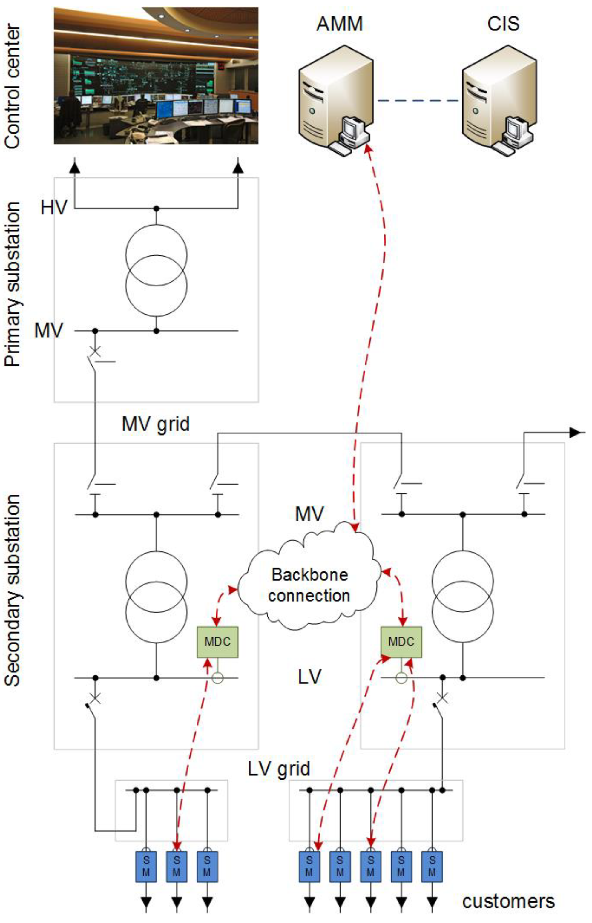
2.1. Review of the 1st Generation AMI in Italy

AMIs are now deployed in several European Countries [24,25] and the rest of the world [26,27,28,29]. In Italy, SMs installation started in 2003 and became mandatory with the resolution 292/06 of the Italian Regulatory Authority for Energy, Networks and Environment (ARERA). SMs are mainly used for customer relationship management:
  • Activation/deactivation of contracts
  • Contractual power changes
  • Power curtailment
  • Anti-tampering
  • Monthly reading of energy counters for billing
Concerning the measurement and collection of real-time measurements and power profiles, AMIs generally present some constraints, inherited from the most common implementation architecture (Figure 1), which is composed of:
  • Electronic meters per each customer
  • A Meter Data Concentrator (MDC) collecting customers’ data and installed in secondary substations
  • An Automatic Metering Management (AMM) system, collecting data from MDCs
Contractual information about customers is stored in the Customer Information System (CIS), which is connected to the AMM. When, for example, a contractual power changes, a new task is scheduled about the contract in the CIS and this creates a reconfiguration job for the AMM, which in turn reconfigures the specific SM with the new value.
A first constraint of this architecture is due to the Narrow Band Power Line Communication (NB-PLC), the most common communication technology used by the MDC to read from SMs. Despite providing the best trade-off in terms of cost and performance in urban and semi-urban areas, it has a relatively low throughput and a high latency [30]. For this reason, today’s SMs calculate 15-min power profiles and typically only transfer them to the MDC once a month, and not in real-time.
The technology used for AMM represents the second constraint. Storing the profile for all the customers requires a huge amount of storage, which would be extremely expensive with a non-cloud solution, such as those commonly used for the first generation of AMIs.
The normative requires that only power profiles of customers with contract power over 55 kW must be collected and stored: they represent a limited number considering the overall distribution network. Generally, the DSO does not download the rest of the power profiles, which include residential or small industrial customers with smaller contractual powers (e.g., 16.0, 6.6 or 3.3 kW). To summarize, state-of-the-art AMIs provide power profiles for about 1% of the customers, and, in any case, the infrastructure is not technically designed and sized to manage a large quantity of power profiles. Thus, applications, such as SE algorithms, which require many power profiles should define approaches to generate them, by limiting the total number of additional data to recover from the AMI.

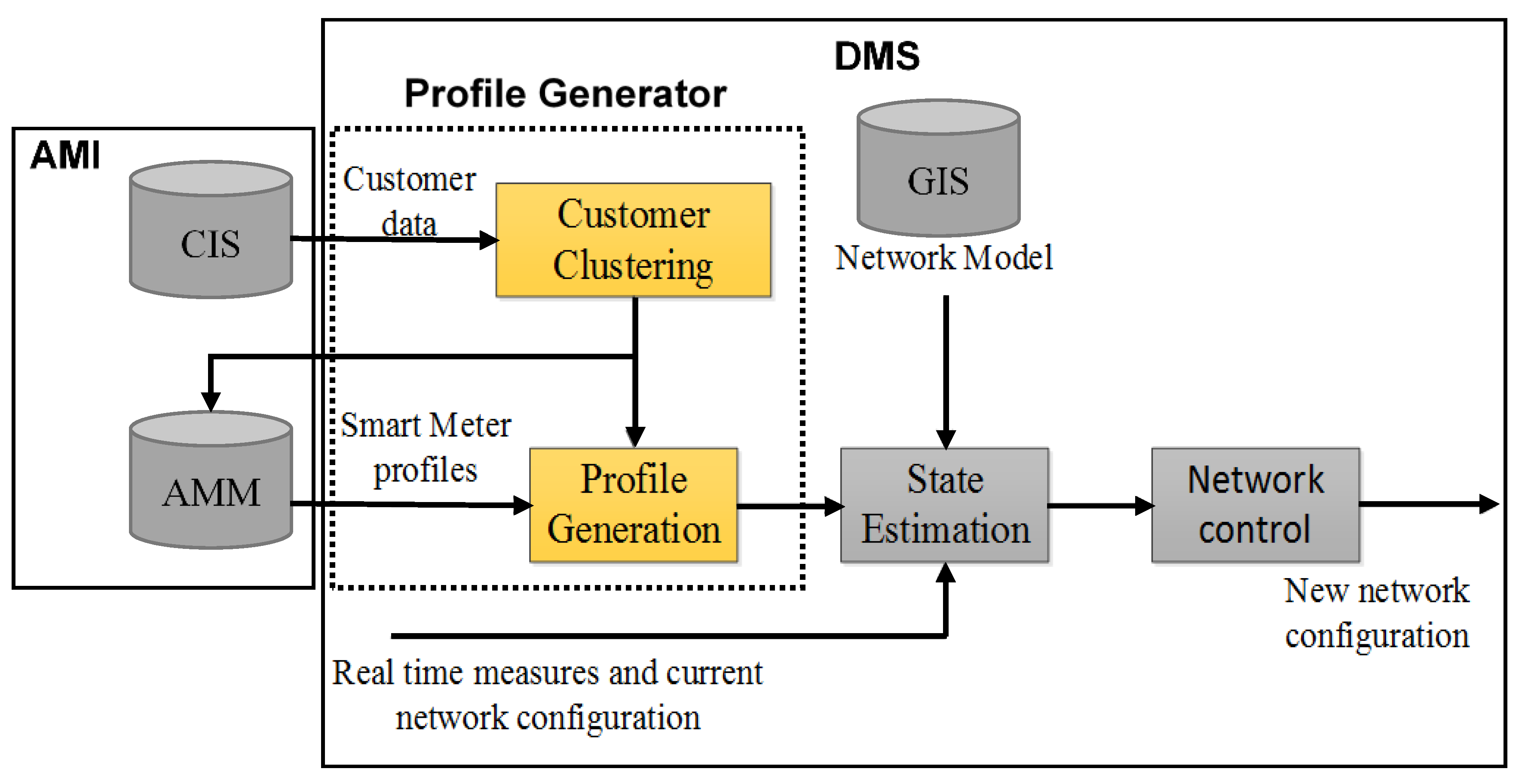
2.2. Profiles Generator

Considering the DSO supervision infrastructure, the SE function is part of the Distribution Management System (DMS), the informative infrastructure used to monitor, manage and configure the distribution network. Generally, SE algorithms are already included as optional add-on in commercial DMS but can be improved by DSO in necessary [31]. In any case, the analysis and study of SE algorithms are out of the scope of the current research, which focuses on the source of data, as detailed in the Introduction. The application of SE algorithm at the LV level requires as many data as possible about the distribution grid, which can be obtained by processing AMI data stored in AMM. Nevertheless, existing AMI infrastructure does not provide power profiles for every connected customer and only a limited number of additional profiles can be recovered from it due to the technical limits highlighted in the previous section. Additional functions are thus required by the DSO informative system in order to recover the required data. The proposed solution to this issue is based on deployment of a profiles generator block, which uses the limited data collected by the AMI system to generate the information required to feed the SE in DMS of the DSO, as shown in Figure 2. This block can be considered as an add-on functionality of the DMS.
More in detail, customers’ data are clustered to identify different classes of customers on the distribution network under analysis. Each cluster is formed by customers with similar characteristics from the DSP point of view. The profile generation function uses the cluster information to download from AMM only a limited number of long-term power profiles for each class of customer. Then, this information is used to estimate the power profiles for all customers who are associated to the same cluster. This information is then provided to the SE algorithm of the DMS.
The diagram in Figure 3 shows the details of the process followed to calculate the power profile for all customers. As a first step, customers’ data are analyzed to identify clusters, i.e., the different classes of customers with the same set of properties (Customer Clustering). Then, power profiles of a sample of customers for each of the classes identified in the previous step are downloaded from the AMI system to generate a normalized power profile for each cluster (Normalized Profile Generation). Finally, power profiles for all customers of each cluster are calculated based on the normalized power profiles estimated in the previous step (Full Profile Generation). The formal description of the process is described in the following section.

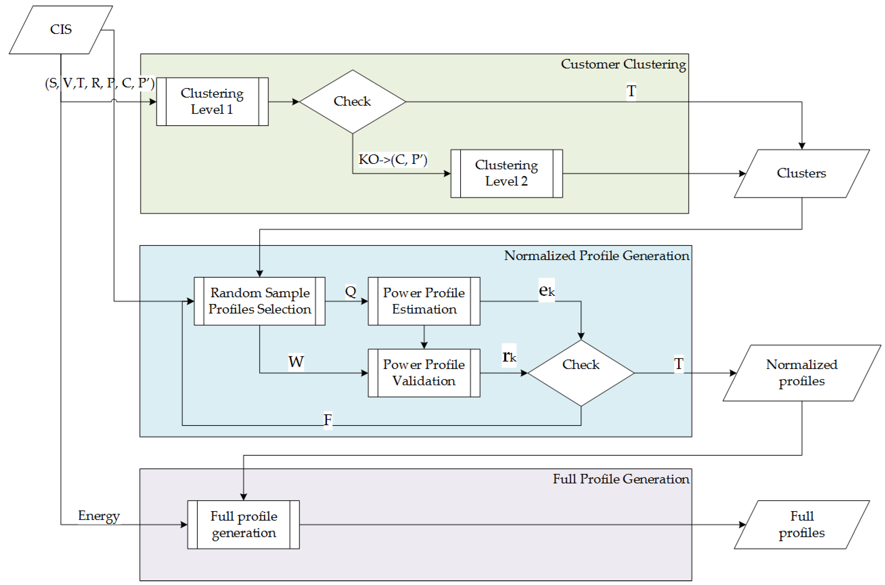
3. The Proposed Approach

3.1. Customer Clustering

The first problem in customer clustering is that the number and features of clusters are not known a priori. In fact, the definition of the correct number of clusters has a strong impact on the time required to process a dataset and the association of customers to the correct cluster. This is why several techniques (among them, those referenced in the Introduction) have the definition of clusters as primary task. However, in the real case when the set of power profiles is not complete, approximations have to be defined and accepted.
The approximation proposed in this paper is to define clusters based on contract information of customers—contained in the CIS—and then to perform further refinement to reach a target accuracy in the model. Examples of contract features which can be taken into consideration for the clustering process are:
  • Customer’s contract status, S = {Connected, Disconnected}
  • Voltage level, V = {LV, MV, HV}
  • Customer’s Contract Type, T = {Residential, Not Residential}
  • Customer’s Type, R = {Consumer, Producer, Prosumer}
  • Contract Power, P = {(0.0, 6.6], (6.6, 16.5], (16.5, 55.0], (55.0, ∞)} kW
  • These parameters are normally stored in CIS systems, therefore clustering based on them is a straightforward and efficient procedure for real-life applications. Besides the above parameters, for each customer, the total energy consumption in a given month is other information which is available in the CIS. Based on that, the total annual consumption E per each customer can also be easily obtained.
  • More formally, let us consider a set of N customers; each customer Xi can be described as a couple:
    X i ( H i , Y i ) ,     i < N
  • where
    -
    Hi = (Si, Vi, Ti, Ri, Pi) is the vector of the contract features of the customer; and
    -
    Y i = { y i , t :   t [ 1 , T ] } , is the time series of mean active power values every 15 min, on the considered time horizon T.
The computational effort of the clustering operation depends on the number of clusters k. In the specific case, the maximum number of clusters, k, is given by the H properties of each customer used to define the clusters:
k = | S | · | V | · | T | · | R | · | P |
where | | represents the cardinality operator of each set. It is evident from (2) that the total number of clusters can increase quickly as the number of features used to cluster the profiles increases. Fortunately, the cardinality of some set of features is limited, and some combinations of parameters are not considered interesting from a practical point of view.
In this paper, an iterative approach is proposed to limit the total number of clusters and, consequently, the resources required to estimate the power profiles. This approach is based on a recursive clustering. During the first round, only the parameters S, V, T, R and P are used to classify the customers and to generate the first subset. In Section 4, it is proved that the assumption of limiting the first level of clustering to this subset of parameters is valid in most of the cases.
The criteria to decide which clusters need a second level of clustering are related to the overall energy associated to the cluster. In details, considering the cluster k of cardinality M (i.e., composed by M customer), the total energy Ek associated to the cluster k is defined as:
E k = m = 1 M E m
where Em represents the total annual energy of the mth customer of the cluster k, whose value is stored in CIS. Considering the distribution of the Ek population, whose standard deviation is σ E , those clusters fulfilling the condition:
E k > 3 σ E
are those that need the second level clustering. Clusters characterized by a large energy exchange with the distribution network are those that provide a larger contribution to the SE algorithms. Therefore, it is reasonable to balance the total energy associated per each cluster using sub-clustering. A more detailed clustering makes the customers more homogenous, improving the accuracy in the estimation of customers’ power profile. Using the sub-clustering approach allows, at the same time, to guarantee a proper trade-off between the accuracy of power profile estimator and the required computational effort.

3.2. Normalized Profile Generation

Considering a cluster, k, of cardinality M (where M < N), the estimator, Y k ^ , of the power profile (in the following power profile estimator), is defined as:
Y k ^ = { q = 1 Q y q , t Q :   t T }
i.e., it is obtained by randomly-selecting a subset Q of power profiles of the cluster k and performing their statistical average.
Q is set as min(QS, M) and corresponds to the number of profiles processed to obtain the estimated profile, for each cluster. QS is a design parameter, and its value represents a trade-off between accuracy and the fact that the number of available profiles is limited. The higher is QS. the more accurate is the estimation of the power profile. If Qs is too high, it is not possible to calculate the error due to a lack of profiles. In the present paper, it is assumed Qs = 100.
The index generally used in statistic to estimate the quality of an estimator is the Root Mean Square Error (RMSE), the square root of the “second sample moment” of the difference between the expected values and the observed values. This quantity is referred as “residuals” when calculations are performed over the data sample used for estimation and is referred as “errors” (or prediction errors) when computed out-of-sample.
Considering the power profile estimator of the cluster k, Y k ^ , the total residual, rk, is calculated as:
r k ( Y k ^ ) = 1 P k q = 1 Q r k , q ( Y k ^ ) Q
where r k , q ( Y k ^ ) = t = 1 T ( y t ^ y q , t ) 2 T represents the residual of the qth power profile of the cluster k. The normalization factor Pk = sup{Pm}M is the upper bound of contractual power among the M customers belonging to the cluster k, and it is introduced to compare residuals among different clusters, which in general have different contractual powers.
The use of a limited number (M) of power profiles, Y k , during the estimation process could polarize the power profile estimator, Y k ^ . Thus, a subset, Wk, of power profiles is randomly selected from each cluster k, to validate the estimator. In this way, the polarization of the estimator with the respect to the behavior of specific power profiles is largely avoided. The number of power profiles required for the validation is obtained as Wk = min(W, Mk−Qk), where Mk is the cardinality of the cluster k and Qk is the number of power profiles used to estimate Y k ^ . Considering the trade-off between the statistical validity required by validation phase and the need to reduce the total number of power profiles to be recovered from AMI, the design parameter W can be set to 30. The total error, ek, of the power profile estimator of the cluster k, Y k ^ , with the respect to the Wk validation profiles is calculated as:
e k ( Y k ) ^ = 1 P k w = 1 W e k , w ( Y k ^ ) W
where e k , w ( Y k ^ ) = t = 1 T ( y t ^ y w , t ) 2 T is the error of the wth power profile of the cluster k. The power profile estimator of the cluster k, Y k ^ , is considered valid if the following relationship is verified:
| e k ( Y k ^ ) r k ( Y k ^ ) |   ε
where ε is the tolerated deviation of the validation power profiles with the respect to the estimator. The threshold ε is used during the validation phase to assess if the estimated power profile is able to represent with the proper accuracy the cluster to which it belongs, avoiding possible polarization or over-estimating effect due to the limited number of power profiles used. In our analysis, ε was set to 0.05. If the deviation of the validation power profiles is greater than this value, it means the power profiles selection mechanism polarizes the estimator Y k ^ . Thus, the power profile selection process has to be executed again to define a new training set (see Figure 3), increasing the number of power profiles to recover from AMI.
After the validation, each estimated profile, Y k ^ , has to be normalized by its own energy. Each estimated profile, Y k ^ can be monthly partitioned, as:
Y k ^ ( t ) = s = s 1 s 12 Y k ^ ( t ) | t s = s = s 1 s 12 Y k s ^
where the set s = {s1, …, s12}, represents the months in the considered year (please note how sx is not an integer index but is the set of days of the xth month). The energy of the sth month, E k ^ s , of the estimated power profile, Y k ^ , is defined as:
E k ^ s = t = 1 T y k s ^ ( t ) · Δ t ,     t   s
where Δt is the time interval between two consecutive power profile samples (i.e., 15 min in the considered case). The normalized estimator is thus defined as:
Y k , N ^ ( t ) = s = s 1 s 12 Y k s ^ E k ^ s  

3.3. Full Profiles Generation

The third step is responsible for the generation of an estimation of the power profile for each of the customer, using the reference normalized estimator, Y k , N ^ , obtained during the previous step. The power profile for the mth customer of a cluster k, Y k , m ^ , is obtained by scaling the normalized estimator by the energy consumed by that customer on each month of the year, data that are directly available from CIS.
Each normalized estimator Y k , N ^ can be monthly partitioned, as:
Y k , N ^ ( t ) = s = s 1 s 12 Y k , N ^ ( t ) | t s
where the set s = {s1, …, s12}, represents the months in the considered year (please note how sx is not an integer index but is the set of days of the xth month). The full profile associated to the mth customer of the cluster k is thus defined as:
Y k , m ^ ( t ) = s = s 1 s 12 ( Y k , N ^ ( t ) | t s · E k , m s )
where E k , m s represents the total energy consumed by the mth customer of the cluster k during the sth month. This procedure is applied for each customer of each k cluster obtained from Step 1.

4. Results

The aim of this section is to validate the approach described in Section 3 under realistic conditions. The AMI system of Unareti S.p.A. was used as a source of data to be used to estimate full power profile estimators. The following analysis was performed on the distribution network of Lombardy region, in northern Italy, formed by approximately one million customers. The clustering phase was based on real customer data downloaded from the CIS database of the DSO, part of the Distribution Management System (DMS). Unless specified otherwise, the results were obtained from data collected during 2019–2020 (12 months).

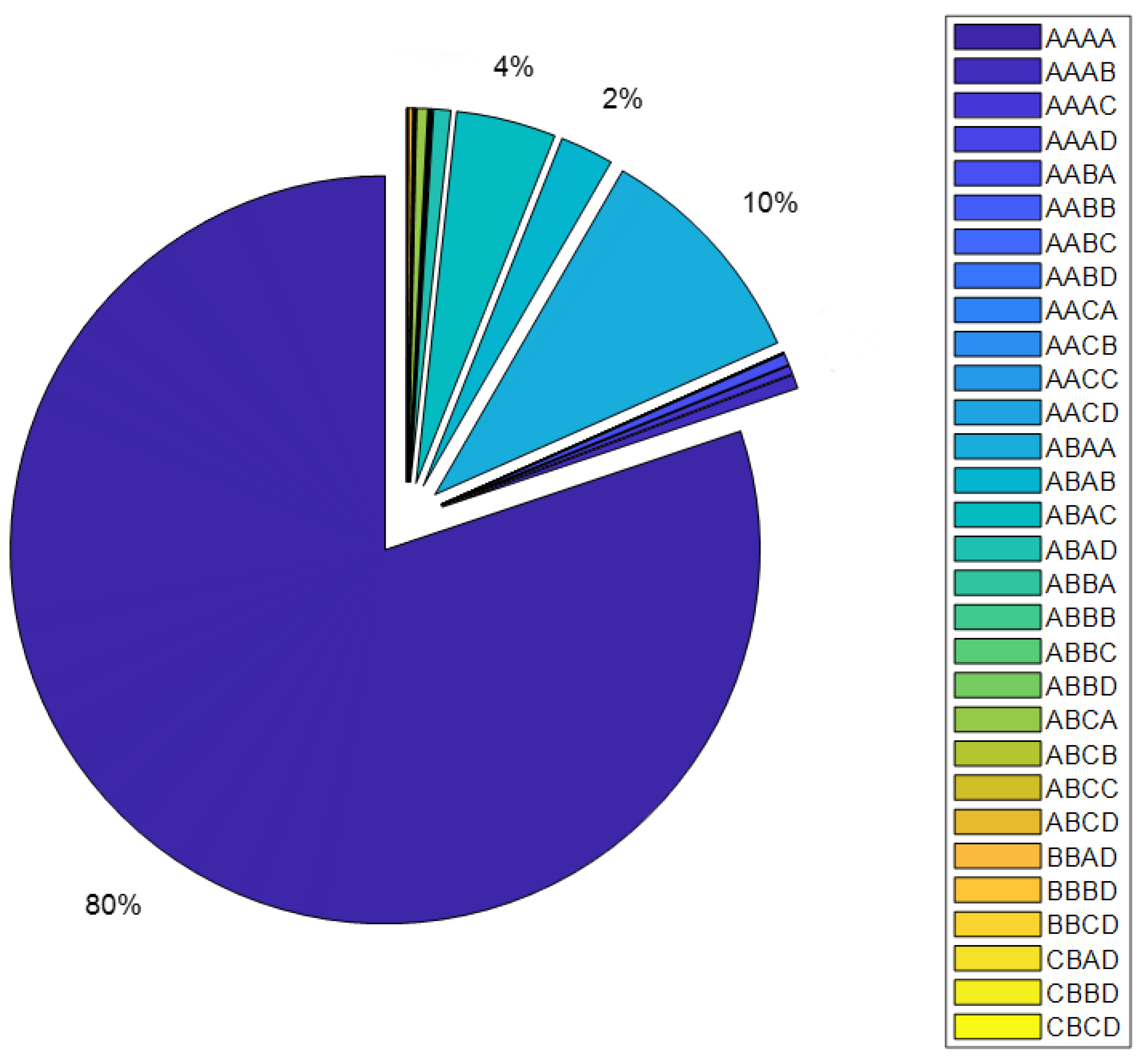
4.1. Customer Clustering

4.1.1. First Level of Clustering

This first level of clustering is applied to all customers and it classifies them based on a subset of features available in CIS: Contract Features S (“Connected” case only), V, T, R and P. The result of first level clustering is 29 clusters, as shown in Table 1. As shown by the data, the distribution of customers per each cluster is different. In particular, the cluster AAAA, i.e., the one associated to “LV, Domestic, Consumer, Contract power less than 6.6 kW”, groups approximately 80% of the total number of customers. As shown in Figure 4, the rest of the clusters share the remaining 20%, considering that the cluster ABAA groups approximately another 10% of customers. Nevertheless, the cardinality of a cluster is not the main parameter to be considered during the clustering phase given the specific application (i.e., grid SE). In fact, from a SE point of view, it is more relevant to consider the total annual energy exchanged by each cluster, as it is an index of the impact of such cluster on the grid behavior. This means that clusters with a “significant” total annual energy are the candidates for a further clustering phase. More formally, the standard deviation of the total energy exchanged per each cluster is 0.48 GWh, which means that the cluster with a total energy per year above 1.44 GWh, as defined from Condition (4), should be further processed.
As can be seen from the total annual energy distribution shown in Figure 5, this is the case of clusters AAAA and BBAD representing approximately half of the total energy exchanged with the power grid. The rest of the energy is distributed almost equally among seven clusters. However, the BBAD cluster is composed of customers with a contractual power above 55 kW. For this class, as recalled in Section 2.1, power profile are available for each customer. The process of the power profile generation in this case can be used to compensate any missing data in the record. Thus, only the AAAA cluster requires a sub-clustering.

4.1.2. Second Level of Clustering

The second level of clustering is performed only on cluster AAAA that includes 80.1% of all customers (S = Connected; V = LV; T = Domestic; R = Consumer; P = (0.0, 6.6] kW) and 21% of the total energy consumed per year by the customers of the DSO.
Two further features are considered for the sub-clustering:
  • City Class based on the density i.e., Number of customers per city C = {
    (500,000, 1,500,000] (the City of Milano),
    (10,000, 500,000] (the City of Brescia),
    (20,000, 100,000] (medium size cities),
    (5000, 20,000] (small towns near a bigger city),
    (0, 5000] (villages in rural areas)}
  • A more granular set of contract powers: P’ = {
    (0.0, 3.3];
    (3.3, 4.4];
    (4.4, 5.5];
    (5.5, 6.6]} kW
The sub-clustering splits the cluster AAAA into 20 sub-clusters. The percentage of customers and the percentage of total annual energy consumed per each sub-cluster are summarized in Table 2. As clearly highlighted by the data in the table, the sub-cluster AAAA-BA is grouping more than 67.91% of the total customers of the AAAA cluster, and it represents, approximately, 65% of the total energy consumption of the original cluster. This result is expected, since this sub-cluster groups the most common contract (contractual power P in (3.3, 4.4]) in the area of the city of Milan, the most populous city managed by the DSO.
Thus, the clusters considered by the generation of the normalized estimator are those indicated in Table 1 and Table 2.

4.2. Normalized Profile Generation

The identification of the customer’ clusters is preparatory for the estimation of the power profile phase. The power profiles of each cluster k are processed to produce as an output the power profile estimator, Y k ^ . As mentioned in Section 3, two metrics are used to validate the quality of this estimator:
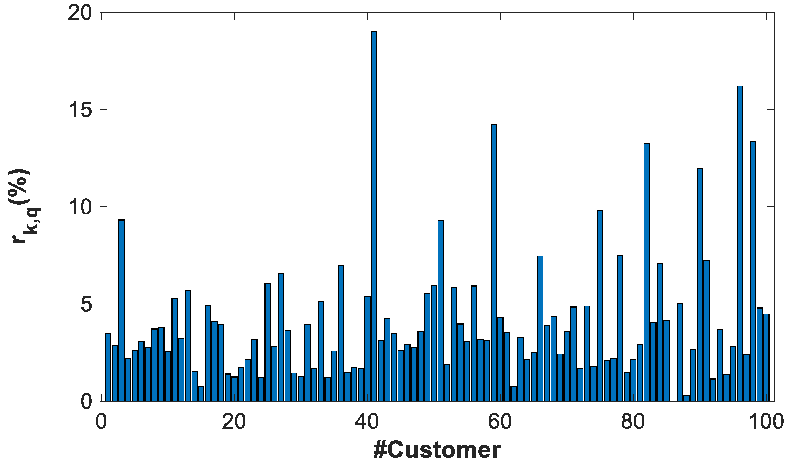
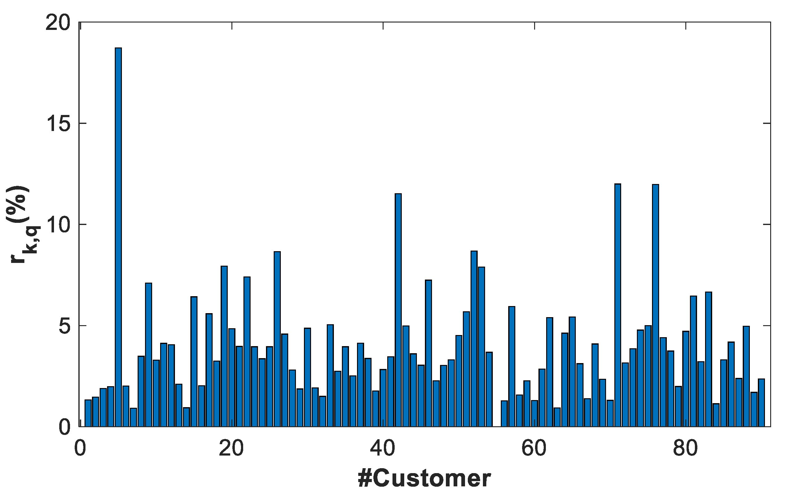
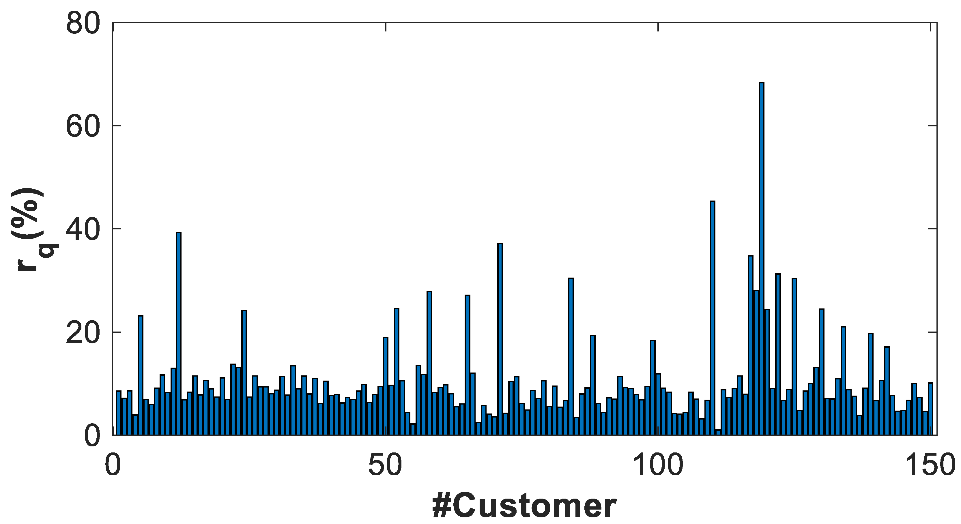
  • The residual describes the variability of the power profile estimator with respect to the power profiles used to calculate it.
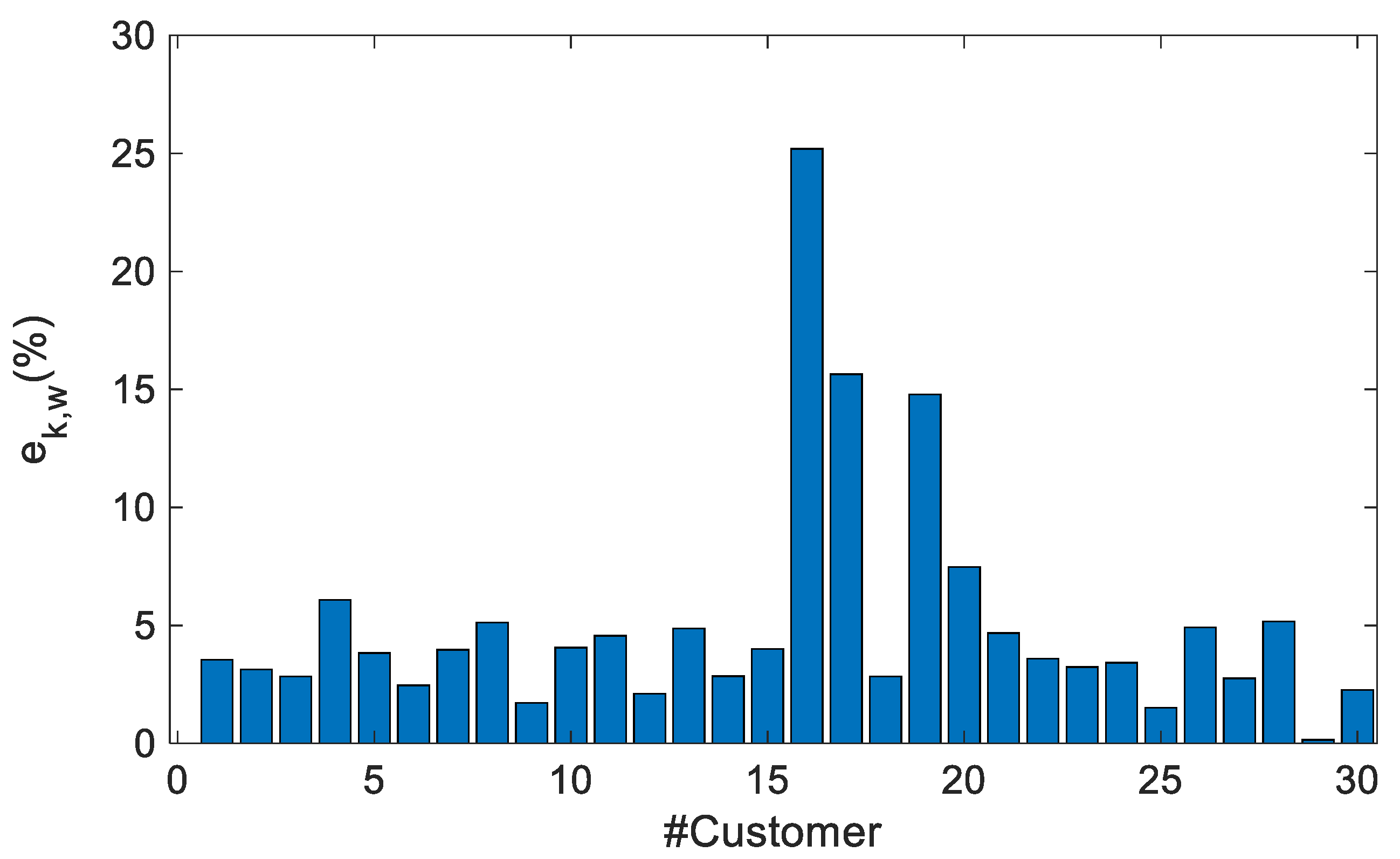
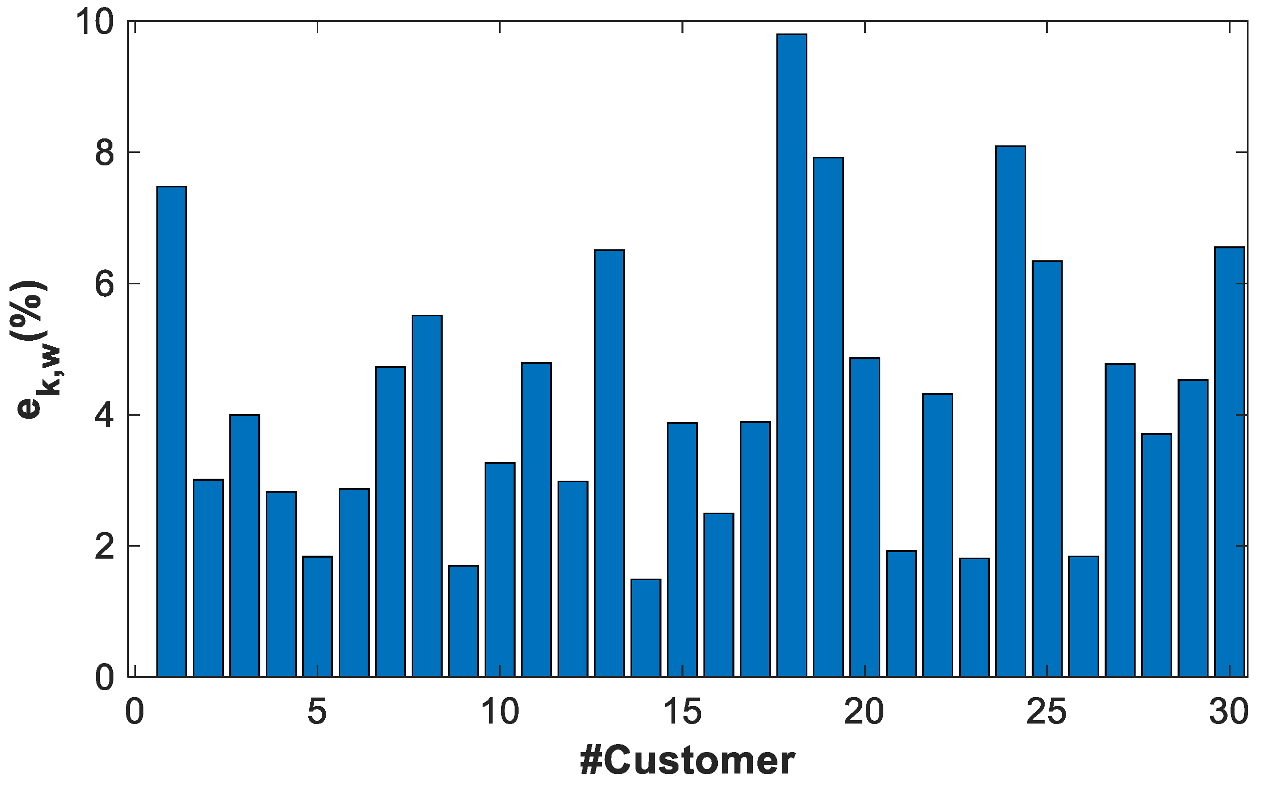
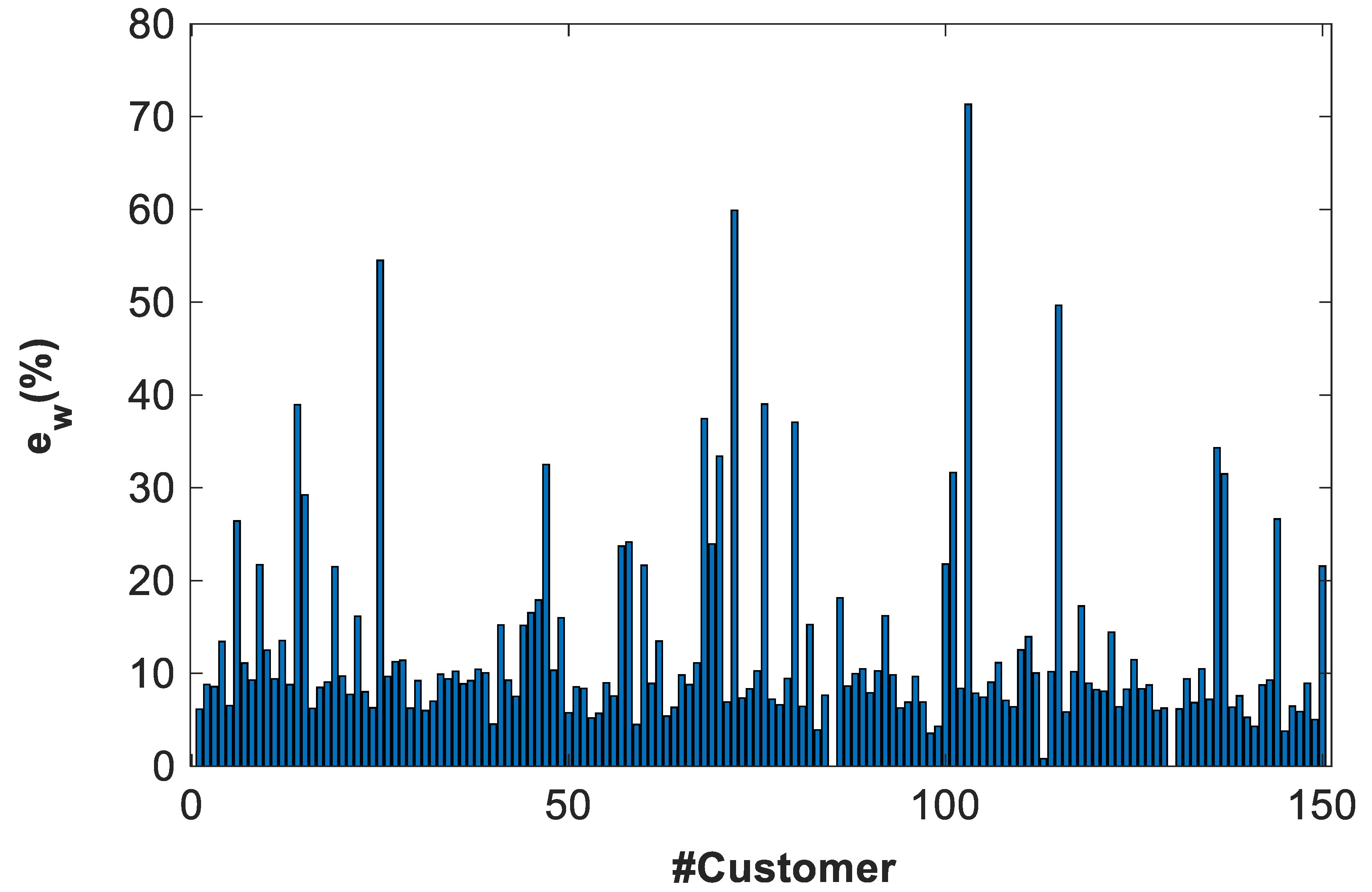
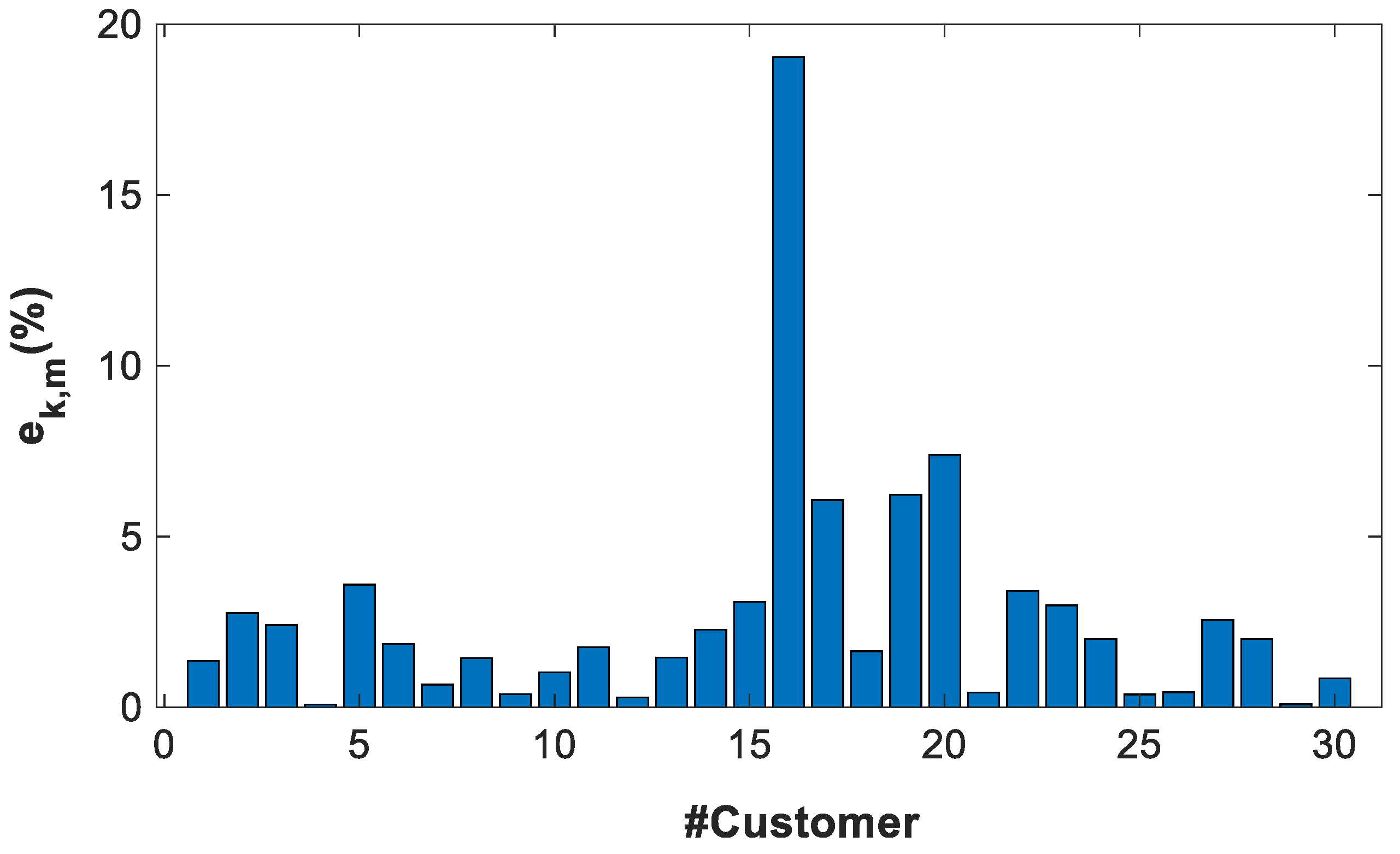
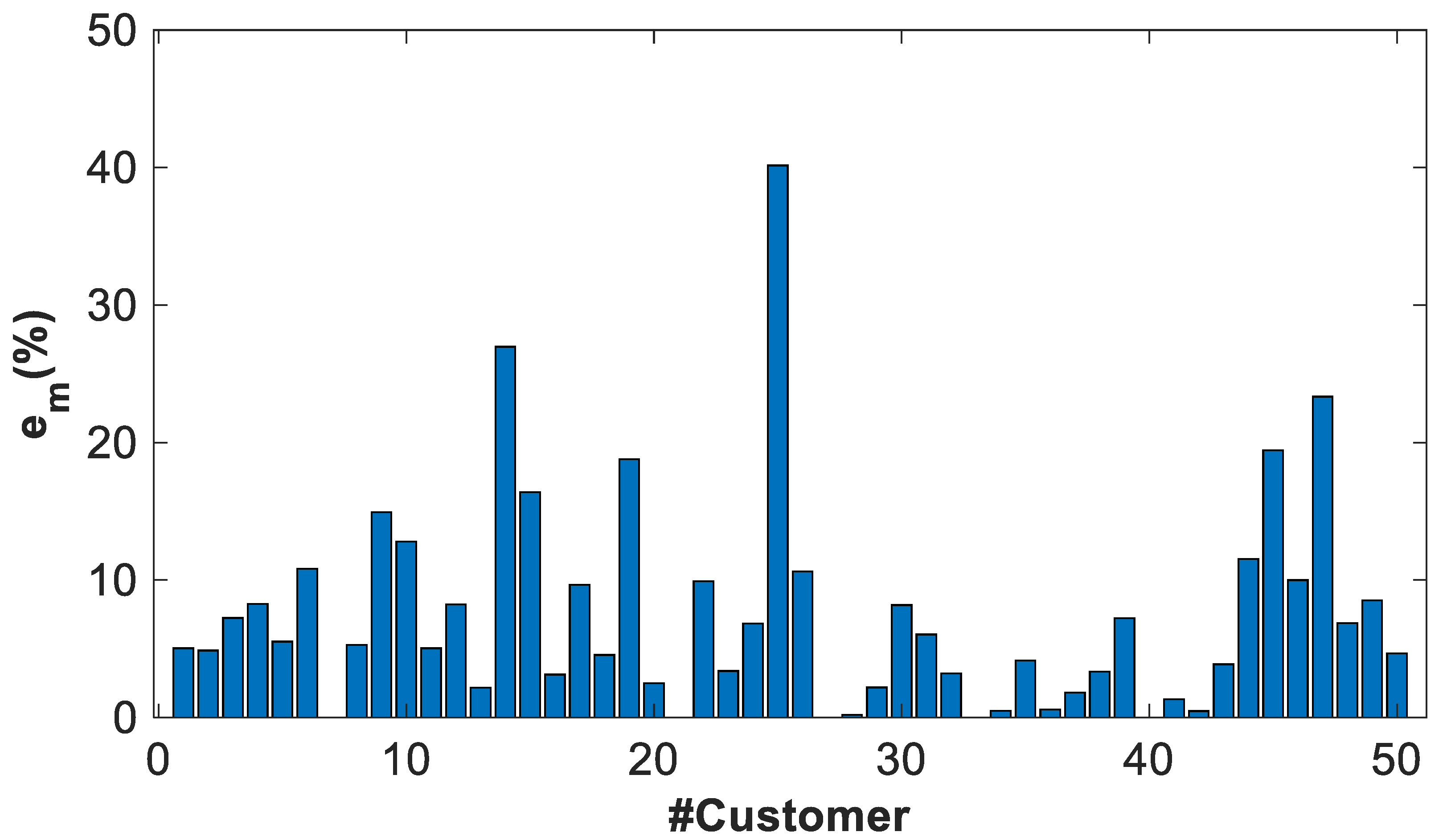
  • The error describes the variability of the power profile estimator with the respect to validation power profiles, different from the previous one.
In the following, a Level 1 cluster (ABAB) and a Level 2 sub-cluster (AAAA-BA) are presented and analyzed as an example of this process. These results are then compared with an algorithm which does not take into account the customers’ clusters.

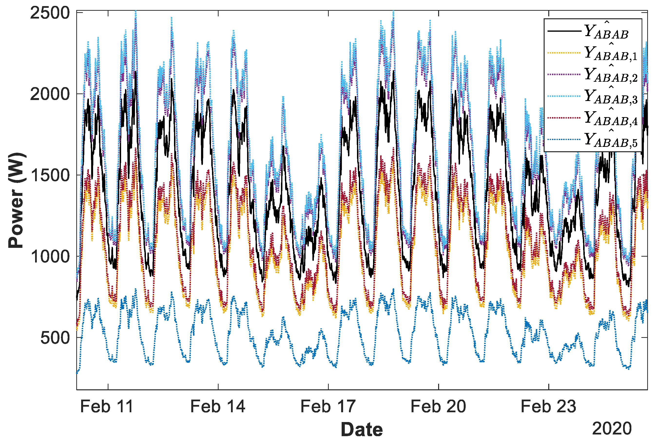
4.2.1. Example of Cluster ABAB

Let us consider the cluster ABAB. QS = 100 power profiles are used to compute the power profile estimator of the cluster, following Equation (5). The partial residual is shown in Figure 6, where it is normalized by the contractual power of the cluster (PABAB A = 16.5 kW). As shown in the figure, it is generally within 5%, although some of the power profiles used during the estimation exhibit a larger value (between 10% and 20% of the contractual power). The total residual, r k ( Y k ^ ) , of the cluster ABAB is 5.4%.
After the elaboration phase, the power profile estimator is validated versus WABAB = 30 power profiles, which differ from those used in the previous phase. Under this condition, it is possible to identify any possible polarization effects. The partial error of the power profile estimator of cluster ABAB with the respect to the validation power profiles is shown in Figure 7, where it is normalized by the contractual power of the cluster PABABA. The partial error is generally below 5%. The partial error is above 10% in few cases (in one case around the 25%). The total error, e k ( Y k ^ ) , is 6.4%. It should be noted that the condition expressed by (8) is satisfied, since the total error of power profile estimator is lower than 5% of the total residual. Thus, the power profile estimator of the cluster ABAB is not polarized. Figure 8 shows the power profile estimator of class ABAB during 11–25 February 2020.

4.2.2. Example of Cluster AAAA-BA

The same approach is used for the sub-cluster AAAA-BA with QS = 100, WAAAA-BA = 30 and considering the contractual power PAAAA-BA = 4 kW for the sake of normalization. The partial residual of the power profile estimator and the related partial error are shown in Figure 9 and Figure 10, respectively. The total residual, r k ( Y k ^ ) is 4.97%, while the total error, e k ( Y k ^ ) is 4.9%. It should be noted that the condition expressed by (8) is satisfied, since the error is lower than the residual. This result can be explained since the validation was performed on a smaller number of power profiles if compared to those used during the estimation phase. Figure 11 shows the power profile estimator of class AAAA-BA during 11–25 February 2020.

4.2.3. Reference Algorithm

Let us consider a subset of 150 power profiles randomly selected among the customers with contract power less than 16.5 kW, representing a large part of the distribution network. In this case, the algorithm does not take into account the clustering phase. The randomly selected 150 power profiles are used to compute the power profile estimator of the considered network, following Equation (5). The partial residual is shown in Figure 12, where it is normalized by the upper bound of contract power of the considered subset (i.e., P= 16.5 kW). As shown in the figure, it is generally less than 20%, although some of the power profiles used during the estimation exhibit a larger value (up to the 70% of the contract power). The total residual, r ( Y ^ ) , is 18.2%, approximately four time the results which can be obtained through the proposed approach.
After the elaboration phase, the power profile estimator is validated versus 150 power profiles, which differ from those used in the previous phase. Under this condition, it is possible to identify any possible polarization effects. The partial error of the power profile estimator with the respect to the validation power profiles is shown in Figure 13, where it is normalized by the upper bound of the contract power of the considered subset (i.e., P = 16.5 kW). The partial error is generally below 20%. The total error is 16.88%.

4.2.4. General Results

The total residual and error of the power profiles estimator, Y k ^ , of a subset of the clusters (obtained at both Level 1 and Level 2 of sub-clustering) is summarized in Table 3. It should be noted that, in all the cases, Condition (8) is satisfied. That is, the total error obtained during the validation phase of the power profile estimator of each cluster is always lower than 5% of the total residual obtained during the estimation phase. That means the power profile estimators of the clusters shown in the table are not polarized by the power profiles used during the estimation phase. Comparing the obtained results with an algorithm which does not take into account the clustering phase, it should be noted that the clustering approach significantly reduce the error of the estimator power profile at the cost of a limited additional number of power profiles.

4.3. Full Profile Generation

The power profiles estimators, Y k ^ , of each cluster k, are normalized by the monthly energy. The so-obtained normalized estimator is then scaled by the monthly energy exchanged by the mth customer (m ∈ [1, M], where M is the cardinality of each cluster k), to synthesize the m full power profiles, Y k , m ^ .
At this stage, no further corrections can be done on the generated full profiles. Nonetheless, it is interesting to evaluate the overall accuracy of this final result, by introducing two indexes: the partial error, e k , m ( Y k . m ^ ) , measuring the distance between the full power profiles, Y k , m ^ , and the measured power profiles, Yk,m, and the overall metric for the cluster “total error”, e k ( Y k . m ^ ) , are defined as
e k ( Y k , m ^ ) = 1 P k m = 1 M e k , m ( Y k , m ^ ) M ;   e k , m ( Y k , m ^ ) = t = 1 T ( y m , t ^ y m , t ) 2 T
Obviously, e k ( Y k , m ^ ) can only be estimated because a limited number of measured power profiles, Yk,m, is available per each cluster k. The estimation of e k ( Y k , m ^ ) is performed using the Wk power profiles used during validation phase in order to get consistent results.
The full power profiles of the cluster k, Y k . m ^ , are considered valid if the following relationship is verified:
e k ( Y k , m ^ )   e k ( Y k ^ )
meaning the full power profiles are able to minimize the error introduce by the power profile estimator Y k ^ .
The limit of this metric is related to the fact that it can be calculated only for Wk times, since these is the number of real profile available for checking the performance of the system. For the remaining population of power profiles which are not available, a second—less accurate—metric can be introduced. Considering the full power profiles, Y k , m ^ , and the power profile estimator, Y k ^ , of the cluster k, the total deviation, dk, and the partial deviation, dk,m, are obtained as
d k ( Y k , m ^ ) = 1 P k   m = 1 M d k , m ( Y k ^ ) M ;   d k , m ( Y k , m ^ ) = t = 1 T ( y t ^ y m , t ^ ) 2 T

4.3.1. Example of Cluster ABAB

Figure 14 shows the power profile estimator Y A B A B ^ (solid black line) of cluster ABAB and a set of five full power profiles (dotted line), Y A B A B , m ^ , during 11–25 February 2020. It should be noted that the full profile represents a scaled version of the power profile estimator, so that the monthly energy exchanged by each mth full power profiles corresponds to the monthly energy exchanged by the mth customer.
The partial deviation of the full profiles of cluster ABAB is shown in Figure 15, normalized by the contractual power of the cluster (PABABA = 16.5 kW). As shown in the figure, it is generally within 5%, although some of the full power profiles exhibit a larger deviation (around the 15%). The total deviation, d k ( Y k . m ^ ) , of the cluster ABAB, is 5.1%.
Similarly, the partial error of the full power profiles of cluster ABAB with the respect to the corresponding measured power profiles is shown in Figure 16, estimated over the WABAB = 30 power profiles used during the validation phase. It is around the 15% just in one case, while it is above 5% in three cases. The total error, e k ( Y k , m ^ ) , of the cluster ABAB is 4%. It should be noted that the condition expressed by (15) is satisfied, since the total error of full profiles is below the total error of the profile estimator of the cluster ABAB (i.e., 6.4%).

4.3.2. Example of Cluster AAAA-BA

The same metrics were calculated on the power profiles obtained from the sub-cluster AAAA-BA.
As shown in Figure 17, the partial deviation (PAAAA-BA = 4 kW) is generally within 5%, although some of the full power profiles exhibit a larger deviation (in any case below 10%). The total deviation, d k ( Y k . m ^ ) , of the sub-cluster AAAA-BA, is 2.9%.
Similarly, the error of the sub-cluster, calculated with WABAB = 30, is shown in Figure 18, which is always below 10%. The error is more equally distributed with the respect to the error of the cluster ABAB. The total error, e k ( Y k , m ^ ) , of the cluster AAAA-BA is 4.2%. It should be noted that the condition expressed by (15) is satisfied also in this case, since the total error of full profiles is below the total error of the profile estimator of the cluster AAAA-BA (i.e., 4.9%).

4.3.3. Reference Algorithm

The same metrics were calculated on a subset of 50 power profiles randomly selected among the customers with contract power less than 16.5 kW. In this case, the algorithm does not take into account the clustering phase. As shown in Figure 19, the partial deviation is generally below 15%, although some of the full power profiles exhibit a larger deviation (around 80%). The total deviation, d ( Y ^ ) , is 19.8%.
Similarly, the error, calculated with a total number of reference power profiles equal to 50, is shown in Figure 20, and it is always below 20%. The total error, e ( Y ^ ) is 12.8%, approximately three time the error obtained using the proposed approach.

4.3.4. General Results

The results of the analysis, in terms of total deviation, e k ( Y k , m ^ ) , and total error, e k ( Y k , m ^ ) , on a subset of the clusters are summarized in Table 4. Looking at the table, the condition defined in (15) is always validated, i.e., the total error of the full profiles is always less than the total error of the power profile estimator. It should be highlighted that the reduction of the error of the full power profiles with the respect to the power profile estimator is, generally, higher in the cluster characterized by a larger deviation. This result is rather easy to explain. Clusters characterized by a large value of deviation have a large distribution of monthly energy. The full power profiles are able to compensate this distribution, since they are obtained by scaling the power profile estimator by the monthly energy, resulting in a lower error. Comparing the obtained results with an algorithm which does not take into account the clustering phase, it should be noted that the clustering approach significantly reduces the error of the estimator power profile at the cost of a limited additional number of power profiles.

5. Discussion

The clustering process defined 49 types of cluster, but not all would be used for the power profile generation process because for every customer with contract power greater than 55 kW (12 clusters) load profile are always available and can be directly used for SE algorithms. In that case, the power profile estimator is still useful: it can be used to compensate missing data, if any.
Customers with a contractual power greater than 55 kW, although their number is limited, have a high-energy absorption compared to the total consumption of the network, as demonstrated also by the analysis performed in the paper. Thus, the accuracy of the result of SE algorithms strongly relies on the availability of these profiles: for this reason, the normative requires they are logged and registered by the DSO.
The remaining 37 clusters that would used to generate power profiles include the customers with contract power less or equal than 55 kW. For these customers, load profiles are not always available, therefore load profiles of sample customers have to be requested to the AMI.
The proposed approach takes into consideration the limits of existing AMI systems. Fewer than 5000 annual power profiles (100 power profiles for each of the 49 clusters) are needed, a quantity of information that can be easily managed by any informative system. These profiles are used to generate a profile estimator per each cluster that in turn is used to generate a full power profile per each of the customer of the DSO network. This approach is scalable, since the computational complexity scales linearly with the increase of number of customers. The generation of a full power profiles consists in a simple multiplication of the power profile estimator by the monthly energy value of the specific customer. This approach has the benefits of limiting the number of power profile to be recorded by the AMI, but, at the same time, offers a good approximation of the behavior of the network, since the maximum error is about 6.3%.

6. Conclusions

The management of modern distribution grid requires the most in-depth knowledge of the behavior of customers to properly respond to the increase of emerging energy consumers, for example, EV charging, or to distributed power generators which production depend by the unpredictable behavior of renewable resources, such as wind or sunlight. The AMI system is a precious source of information the DSO could exploit to gather such knowledge, but technical limits of real implementations prevent downloading power profiles for all customers. Thus, the proposed solution is to synthesize a power profile for each customer of the distribution grid managed by the DSO. The process to generate these power profiles takes the use of the information available in CIS and requires the download of a limited number of reference long-term power profiles from the AMI system.
The proposed approach for the generation of a massive number of customer’s power profiles is a three-phase process. In the first phase, the customers are clustered in homogenous groups. The clustering is based on customer’s data contained in CIS database. The clustering phase provides for an iterative approach, which allows sub-clustering the clusters which still exhibit a larger variation in terms of energy exchanged by the customers of that cluster. In the second phase, a limited number of customers is randomly selected to represent each of the clusters. The power profiles of these customers are monitored and logged for a predefined time interval. Then, these power profiles are processed to synthesize the normalized estimator of power profile, representing the average behavior of the customers of each cluster. Finally, the normalized estimator of power profile is scaled by the monthly energy exchanged by each customer of that cluster, to generate a synthesized power profile for each customer. Then, these full power profiles can be used by the DSO for distribution grid management, e.g., as input of SE algorithms.
The validation of this approach was performed using customers’ data of the distribution grid managed by Unareti S.p.A., an Italian DSO. The clustering was performed on more than one million of customers, located in northern Italy. The result of the clustering phase is the definition of 49 clusters, each of them representing a specific class of customers with similar contractual features. The proposed approach allows reducing the total number of long-term power profiles to be recovered from the AMI system: fewer than 5000 annual power profiles (100 power profiles for each of the 49 clusters) are needed for the generation of full power profile estimator.
As a result of the above-mentioned process, the total root mean square error of the synthesized full power profiles with the respect to real power profile is on the order of 6.3%, considering the cluster with largest variability of customers’ energetic behavior. These results demonstrate the validity of the proposed approach, able, at the same time, to limit the total number of real power profiles to be logged from the AMI system and synthesized customers’ power profiles with a proper accuracy.

Author Contributions

D.D.G. and S.R. (Stefano Robustelli) conceived and designed the experiments; S.R. (Stefano Robustelli) performed the experiments; S.R. (Stefano Robustelli) and S.R. (Stefano Rinaldi) analyzed the data; D.D.G. and S.R. (Stefano Rinaldi) wrote the paper; and S.R. (Stefano Robustelli) and A.A. reviewed the paper. All authors have read and agreed to the published version of the manuscript.

Funding

This research received no external funding.

Institutional Review Board Statement

Not applicable.

Informed Consent Statement

Not applicable.

Data Availability Statement

Data available on request due to privacy restrictions.

Conflicts of Interest

The authors declare no conflict of interest.

Nomenclature

SCustomer’s contract status
VVoltage level
TCustomer’s contract type
RCustomer’s type
PContract Power
NTotal number of customers
XiProperties of the ith customer
HiVector of the contract features of the customer
YiMean Active power profiles
TTime horizon
kTotal number of clusters
MCardinality of a cluster
EkTotal energy associated to a cluster k over the time horizon T
EmTotal energy of the mth power profile over the time horizon T
Y k ^ Power profile estimator
QSub-set of power profiles used to estimate Y k ^
QSDesign parameter used to define the actual value of Q
PkUpper bound of contractual power of cluster k
r k , q ( Y k ^ ) The residual of the qth power profile of the cluster k
r k ( Y k ^ ) The normalized total residual of cluster k
WkCardinality of the set of power profiles used for the validation
e k ( Y k ^ ) The normalized total error of cluster k
e k , w ( Y k ^ ) The error of the wth power profile of the cluster k
εTolerated deviation of the validation power profiles with the respect to the estimator
E k ^ Energy of the power profile estimator of cluster k over the time horizon T
Y k , N ^ Normalized power profile estimator
Y k , m ^ Full power profile of the m customer of the cluster k
e k , m ( Y k . m ^ ) 
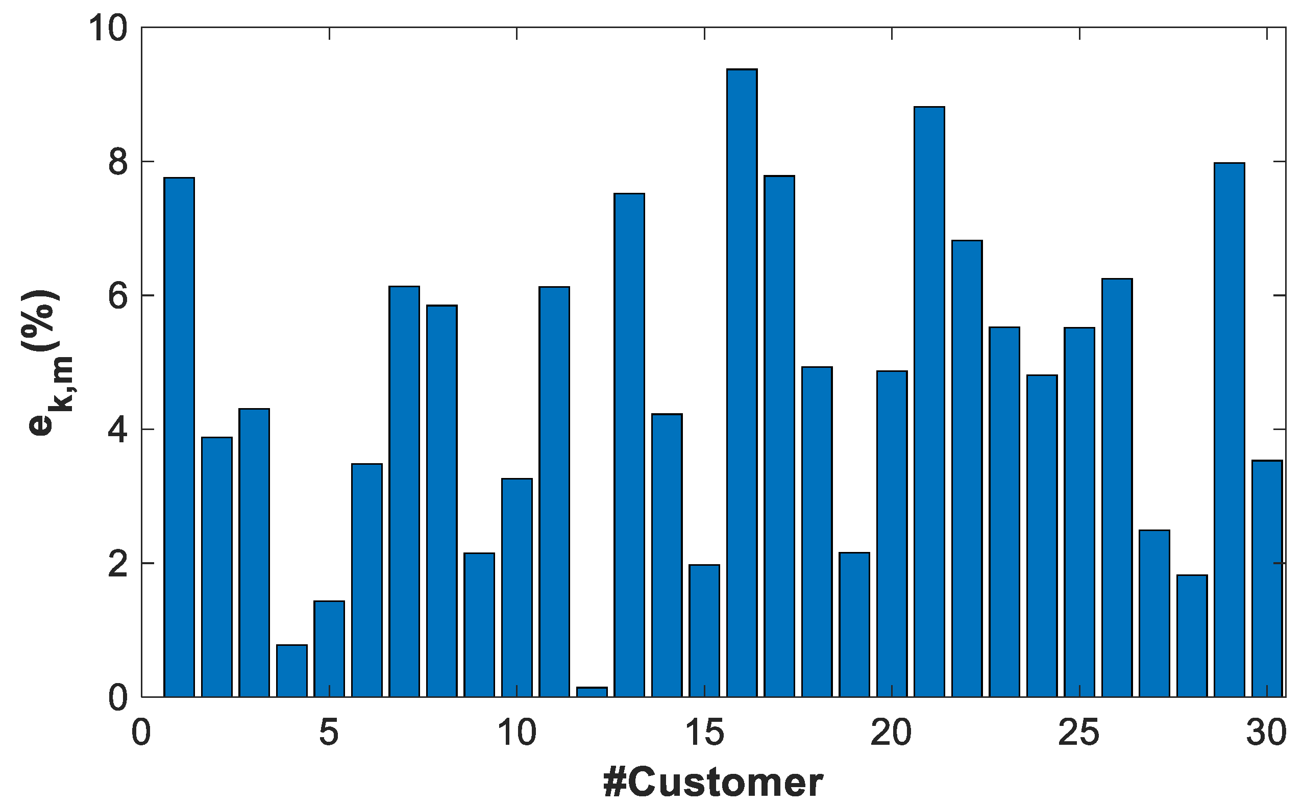
The error of the mth full power profile with the respect to validation power profile
e k ( Y k , m ^ ) The total error of the cluster k in estimating the full power profiles
d k , m ( Y k , m ^ ) 
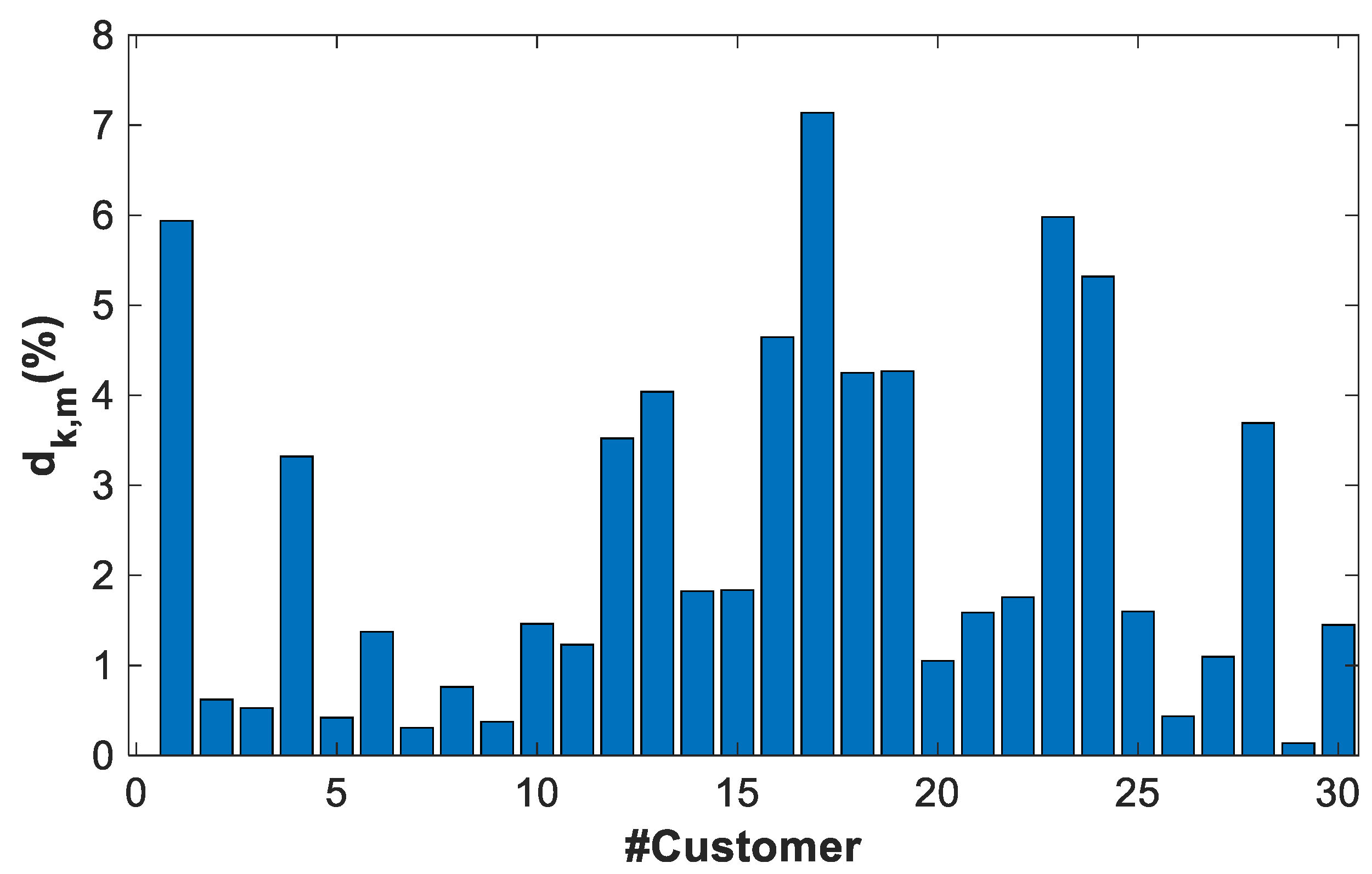
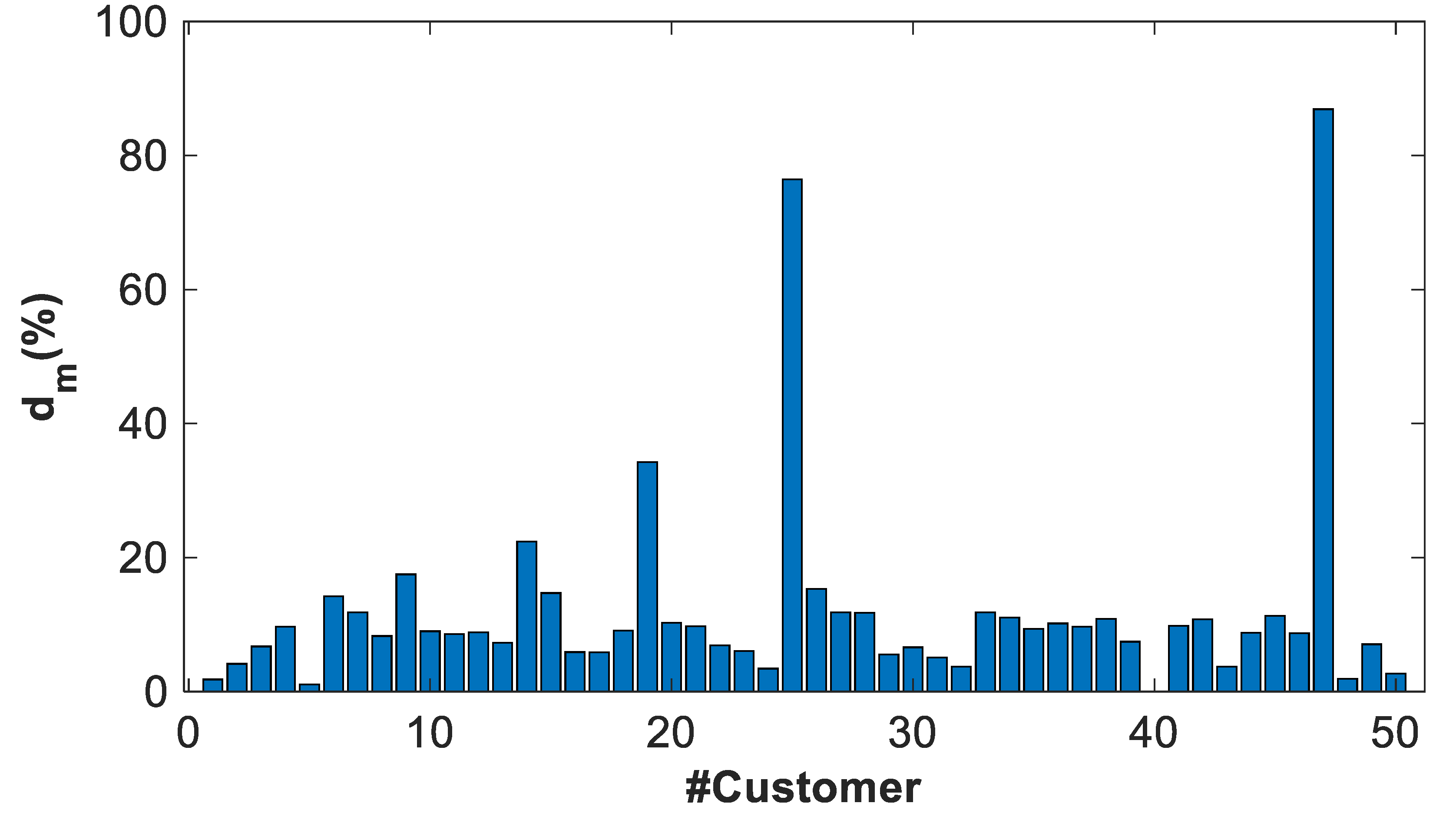
The distance of the mth full power profile with the respect to the power profile estimator
d k ( Y k , m ^ ) The total distance of the full power profiles of the cluster k

References

  1. Repo, S.; Maki, K.; Jarventausta, P.; Samuelsson, O. ADINE—EU demonstration project of active distribution network. In Proceedings of the CIRED Seminar 2008: SmartGrids for Distribution, Frankfurt, Germany, 23–24 June 2008; pp. 1–5. [Google Scholar]
  2. Stanelyte, D.; Radziukynas, V. Review of voltage and reactive power control algorithms in electrical distribution networks. Energies 2019, 13, 58. [Google Scholar] [CrossRef] [Green Version]
  3. Alonso, M.; Amarís, H.; Rojas, B.; Della Giustina, D.; Dedè, A.; AlJassim, Z. Optimal network reconfiguration for congestion management optimization in active distribution networks. In Proceedings of the International Conference on Renewable Energies and Power Quality (ICREPQ-2016), Madrid, Spain, 4–6 May 2016. [Google Scholar]
  4. Tran, Q.T.T.; Sanseverino, E.R.; Zizzo, G.; Di Silvestre, M.L.; Nguyen, T.L.; Tran, Q.-T. Real-time minimization power losses by driven primary regulation in islanded microgrids. Energies 2020, 13, 451. [Google Scholar] [CrossRef] [Green Version]
  5. Kacejko, P.; Adamek, S.; Wydra, M. Optimal voltage control in distribution networks with dispersed generation. In Proceedings of the 2010 IEEE PES Innovative Smart Grid Technologies Conference Europe (ISGT Europe), Gothenberg, Sweden, 11–13 October 2010; pp. 1–4. [Google Scholar] [CrossRef]
  6. Pasetti, M.; Rinaldi, S.; Flammini, A.; Longo, M.; Foiadelli, F. Assessment of electric vehicle charging costs in presence of distributed photovoltaic generation and variable electricity tariffs. Energies 2019, 12, 499. [Google Scholar] [CrossRef] [Green Version]
  7. Aslam, S.; Khalid, A.; Javaid, N. Towards efficient energy management in smart grids considering microgrids with day-ahead energy forecasting. Electr. Power Syst. Res. 2020, 182, 106232. [Google Scholar] [CrossRef]
  8. Pau, M.; Pegoraro, P.A.; Monti, A.; Muscas, C.; Ponci, F.; Sulis, S. Impact of Current and Power Measurements on Distribution System State Estimation Uncertainty. IEEE Trans. Instrum. Meas. 2019, 68, 3992–4002. [Google Scholar] [CrossRef]
  9. Rinaldi, S.; Della Giustina, D.; Ferrari, P.; Flammini, A. Distributed monitoring system for voltage dip classification over distribution grid. Sustain. Energy Grids Netw. 2016, 6, 70–80. [Google Scholar] [CrossRef]
  10. Tosato, P.; Macii, D.; Luiso, M.; Brunelli, D.; Gallo, D.; Landi, C. A Tuned Lightweight Estimation Algorithm for Low-Cost Phasor Measurement Units. IEEE Trans. Instrum. Meas. 2018, 67, 1047–1057. [Google Scholar] [CrossRef]
  11. Leonardi, L.; Battaglia, F.; Bello, L.L. RT-LoRa: A Medium Access Strategy to Support Real-Time Flows over LoRa-Based Networks for Industrial IoT Applications. IEEE Internet Things J. 2019, 6, 10812–10823. [Google Scholar] [CrossRef]
  12. Pasetti, M.; Sisinni, E.; Ferrari, P.; Rinaldi, S.; Depari, A.; Bellagente, P.; Giustina, D.D.; Flammini, A. Evaluation of the use of class B LoraWAn for the coordination of distributed interface protection systems in smart grids. J. Sens. Actuator Netw. 2020, 9, 13. [Google Scholar] [CrossRef] [Green Version]
  13. Wydra, M.; Kubaczynski, P.; Mazur, K.; Ksiezopolski, B. Time-aware monitoring of overhead transmission line sag and temperature with lora communication. Energies 2019, 12, 505. [Google Scholar] [CrossRef] [Green Version]
  14. Hashmi, S.A.; Ali, C.F.; Zafar, S. Internet of things and cloud computing-based energy management system for demand side management in smart grid. Int. J. Energy Res. 2021, 45, 1007–1022. [Google Scholar] [CrossRef]
  15. Albu, M.M.; Sǎnduleac, M.; Stǎnescu, C. Syncretic Use of Smart Meters for Power Quality Monitoring in Emerging Networks. IEEE Trans. Smart Grid 2017, 8, 485–492. [Google Scholar] [CrossRef]
  16. Lukocius, R.; Nakutis, Ž.; Daunoras, V.; Deltuva, R.; Kuzas, P.; Rackiene, R. An analysis of the systematic error of a remote method for a wattmeter adjustment gain estimation in smart grids. Energies 2019, 12, 37. [Google Scholar] [CrossRef] [Green Version]
  17. Nakutis, Z.; Rinaldi, S.; Kuzas, P.; Lukočius, R. A Method for Noninvasive Remote Monitoring of Energy Meter Error Using Power Consumption Profile. IEEE Trans. Instrum. Meas. 2020, 69, 6677–6685. [Google Scholar] [CrossRef]
  18. Rinaldi, S.; Bonafini, F.; Ferrari, P.; Flammini, A.; Sisinni, E.; Cara, D.D.; Panzavecchia, N.; Tine, G.; Cataliotti, A.; Cosentino, V.; et al. Characterization of IP-Based communication for smart grid using software-defined networking. Trans. Instrum. Meas. 2018, 67, 2410–2419. [Google Scholar] [CrossRef]
  19. Artale, G.; Cataliotti, A.; Cosentino, V.; Di Cara, D.; Guaiana, S.; Panzavecchia, N.; Tine, G. Real-Time Power Flow Monitoring and Control System for Microgrids Integration in Islanded Scenarios. IEEE Trans. Ind. Appl. 2019, 55, 7186–7197. [Google Scholar] [CrossRef]
  20. Natale, N.; Pilo, F.; Pisano, G.; Troncia, M.; Bignucolo, F.; Coppo, M.; Pesavento, N.; Turri, R. Assessment of typical residential customers load profiles by using clustering techniques. In Proceedings of the 2017 AEIT International Annual Conference, Cagliari, Italy, 20–22 September 2017; pp. 1–6. [Google Scholar]
  21. Zhong, S.; Tam, K. Hierarchical Classification of Load Profiles Based on Their Characteristic Attributes in Frequency Domain. IEEE Trans. Power Syst. 2015, 30, 2434–2441. [Google Scholar] [CrossRef]
  22. Mutanen, A.; Ruska, M.; Repo, S.; Järventausta, P. Customer Classification and Load Profiling Method for Distribution Systems. IEEE Trans. Power Del. 2011, 26, 1755–1763. [Google Scholar] [CrossRef]
  23. Prahastono, I.; King, D.; Ozveren, C.S. A review of Electricity Load Profile Classification methods. In Proceedings of the 2007 42nd International Universities Power Engineering Conference, Brighton, MA, USA, 4–6 September 2007; pp. 1187–1191. [Google Scholar]
  24. Vasconcelos, J. Survey of Regulatory and technological Development Concerning Smart Metering in the European Union Electricity Market; Policy Papers, RSCAS 2008/01; European University Institute: Florence, Italy, 2008. [Google Scholar]
  25. Marcoci, A.; Raffaelli, S.; Galan, J.M.; Cagno, E.; Micheli, G.J.L.; Mauri, G.; Urban, R.; Grids, S.; Fenosa, U.; Gestionale, D.I. The Meter-ON project: How to support the deployment of advanced metering infrastructures in Europe? In Proceedings of the CIRED, Stockholm, Sweden, 10–13 June 2013; pp. 1–4. [Google Scholar]
  26. Milam, M.; Venayagamoorthy, G.K. Smart meter deployment: US initiatives. In Proceedings of the IEEE ISGT 2014, Washington, DC, USA, 19–22 February 2014; pp. 1–5. [Google Scholar]
  27. Khan, M.F.; Jain, A.; Arunachalam, V.; Paventhan, A. Roadmap for smart metering deployment for Indian smart grid. In Proceedings of the IEEE PES GMCE, National Harbor, MD, USA, 27–31 July 2014; pp. 1–5. [Google Scholar]
  28. Brunekreeft, G.; Luhmann, T.; Menz, T.; Müller, S.-U.; Recknagel, P. Regulatory Pathways for Smart Grid Development in China; Springer Vieweg: Wiesbaden, Germany, 2015; pp. 1–163. [Google Scholar]
  29. Duarte, D.P.; Maia, F.C.; Neto, A.B.; Cesar, L.S.; Kagan, N.; Gouvea, M.R.; Labronici, J.; Guimaraes, D.S.; Bonini, A.; Resende Da Silva, J.F. Brazilian smart grid roadmap—An innovative methodology for proposition and evaluation of smart grid functionalities for highly heterogeneous distribution networks. In Proceedings of the 2013 IEEE PES Conference on Innovative Smart Grid Technologies, Sao Paulo, Brazil, 15–17 April 2013; pp. 1–8. [Google Scholar]
  30. Dedè, A.; Della Giustina, D.; Rinaldi, S.; Ferrari, P.; Flammini, A.; Vezzoli, A. Smart meters as part of a sensor network for monitoring the low voltage grid. In Proceedings of the IEEE Sensors Applications Symposium (SAS), Zadar, Croatia, 13–15 April 2015; pp. 1–6. [Google Scholar]
  31. Energy Management System, Schneider Electric. Available online: https://www.se.com/ww/en/work/solutions/for-business/electric-utilities/energy-management-system-ems/ (accessed on 28 January 2021).
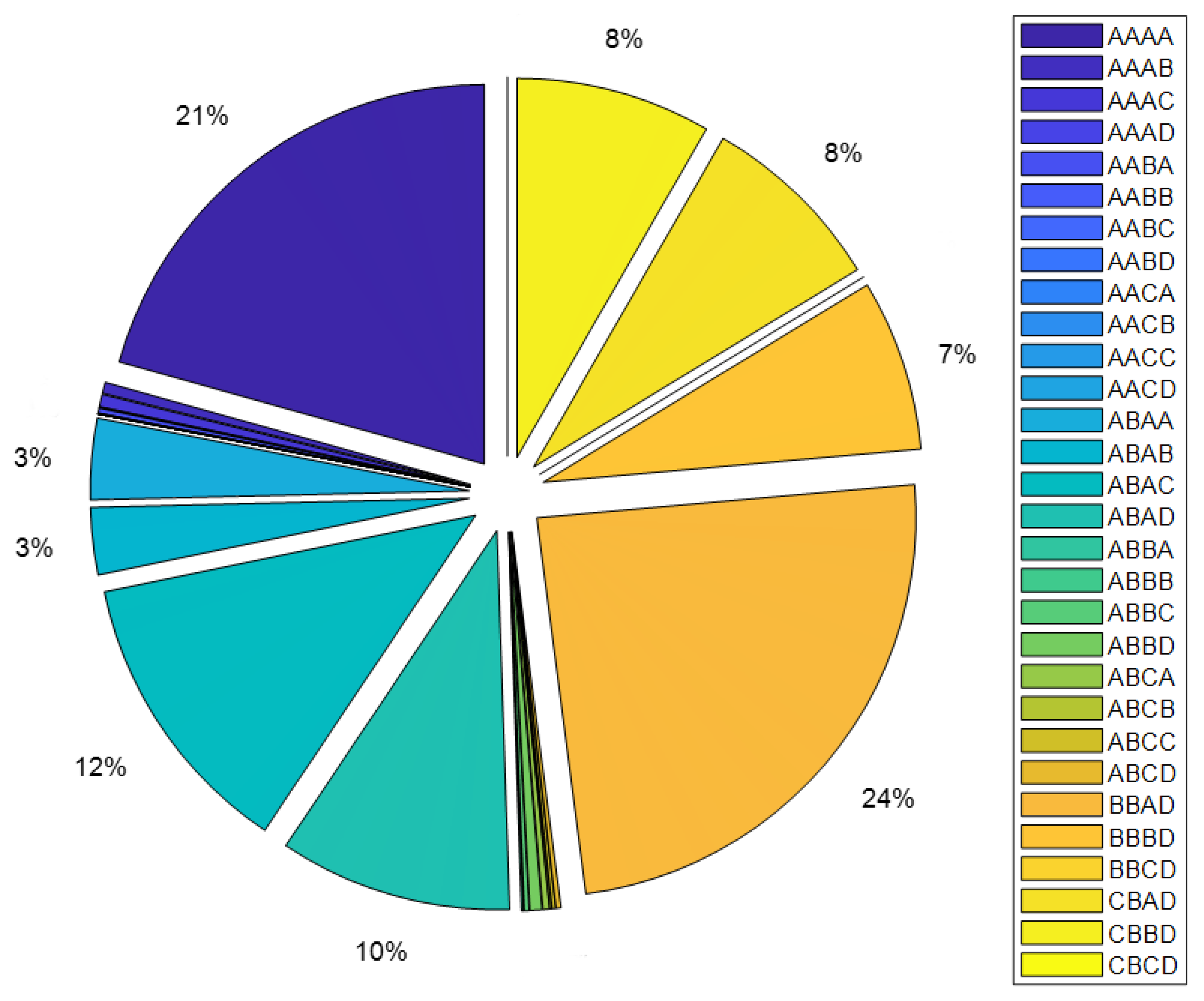
Figure 1. Basic architecture of an Automatic Metering Infrastructure (AMI).
Energies 14 01277 g001
Figure 2. The relationship of customer clustering and power profile generation functions for SE with the respect to existing DSO supervision infrastructures.
Energies 14 01277 g002
Figure 3. The flow diagram used to generate massive power profiles.
Energies 14 01277 g003
Figure 4. The distribution of number of customers per each class.
Energies 14 01277 g004
Figure 5. The percentage of total annual energy consumed by each cluster.
Energies 14 01277 g005
Figure 6. The partial residual of the power profiles estimator, Y A B A B ^ , of cluster k = ABAB. The residual is normalized by the contractual power of the cluster ABAB (PABAB = 16.5 kW).
Energies 14 01277 g006
Figure 7. The partial error of the power profiles estimator, Y A B A B ^ , of cluster k = ABAB. The error is normalized by the contractual power of the cluster ABAB (PABAB = 16.5 kW).
Energies 14 01277 g007
Figure 8. The power profile estimator, Y k ^ , of cluster ABAB during 11–25 February 2020.
Energies 14 01277 g008
Figure 9. The partial residual of the power profiles estimator, Y A A A A - B A ^ , of sub cluster k = AAAA-BA. The residual is normalized by the contractual power of the cluster AAAA-BA (PAAAA-BA = 4 kW).
Energies 14 01277 g009
Figure 10. The partial error of the power profiles estimator, Y A A A A - B A ^ , of cluster k = AAAA-BA. The error is normalized by the contractual power of the cluster AAAA-BA (PAAAA-BA = 4 kW).
Energies 14 01277 g010
Figure 11. The power profile estimator, Y k ^ , of Cluster AAAA-BA during 11–25 February 2020.
Energies 14 01277 g011
Figure 12. The partial residual of the power profiles estimator, Y ^ , obtained using the reference algorithm without the clustering phase. The residual is normalized by the upper bound of the contractual power of the subset of considered power profiles (i.e., P = 16.5 kW).
Energies 14 01277 g012
Figure 13. The partial error of the power profiles estimator, Y ^ , obtained using the reference algorithm without the clustering phase. The error is normalized by normalized by the upper bound of the contractual power of the subset of considered power profiles (i.e., P = 16.5 kW).
Energies 14 01277 g013
Figure 14. Example of a set of full power profiles (dotted line), Y A B A B , m ^ , synthesized from the estimate power profile (solid line), Y A B A B ^ , of the cluster ABAB during 11–25 February 2020. The number of full power profiles is limited to five for sake of clarity.
Energies 14 01277 g014
Figure 15. The partial deviation of the full power profiles, Y A B A B , m ^ , of cluster k = ABAB with the respect to the estimate power profile Y A B A B ^ . The deviation is normalized by the contractual power of the cluster ABAB (PABAB = 16.5 kW).
Energies 14 01277 g015
Figure 16. The partial error of the full energies profiles, Y A B A B , m ^ , of cluster k = ABAB with the respect to the estimate power profile Y A B A B ^ . The error is normalized by the contractual power of the cluster ABAB (PABAB = 16.5 kW).
Energies 14 01277 g016
Figure 17. The partial deviation of the full energies profiles, Y A A A A B A , m ^ , of cluster k = AAAA-BA with the respect to the estimate power profile Y A A A A B A ^ . The deviation is normalized by the contractual power of the cluster AAAA-BA (PAAAA-BA = 4 kW).
Energies 14 01277 g017
Figure 18. The partial error of the full energies profiles, Y A A A A - B A , m ^ , of cluster k = AAAA-BA with the respect to the estimate power profile Y A A A A B A ^ . The error is normalized by the contractual power of the cluster AAAA-BA (PAAAA-BA = 4 kW).
Energies 14 01277 g018
Figure 19. The partial deviation of the full power profiles, Y m ^ , with the respect to the estimate power profile Y ^ , obtained using the reference algorithm without the clustering phase. The deviation is normalized by the upper bound of the contractual power of the subset of considered power profiles (i.e., P = 16.5 kW).
Energies 14 01277 g019
Figure 20. The partial error of the full energies profiles, Y m ^ , with the respect to the estimate power profile Y ^ , obtained using the reference algorithm without the clustering phase. The error is normalized by normalized by the upper bound of the contractual power of the subset of considered power profiles (i.e., P = 16.5 kW).
Energies 14 01277 g020
Table 1. Output of the clustering, Level 1: number of customers, total energy and percentage of total energy consumed in a year per each cluster.
ClusterVTRP (kW)#Customers (%)Ek (GWh)Ek (%)
* AAAALVDomesticConsumer(0.0, 6.6]80.11.5820.7
AAABLVDomesticConsumer(6.6, 16.5]0.60.0360.5
AAACLVDomesticConsumer(16.5, 55.0]0.40.0400.5
** AAADLVDomesticConsumer(55.0, ∞)0.0040.0020.03
AABALVDomesticProsumer(0.0, 6.6]0.50.0160.2
AABBLVDomesticProsumer(6.6, 16.5]0.020.00120.015
AABCLVDomesticProsumer(16.5, 55.0]0.010.00160.02
** AABDLVDomesticProsumer(55.0, ∞)00.000030
AACALVDomesticProducer(0.0, 6.6]000
AACBLVDomesticProducer(6.6, 16.5]000
AACCLVDomesticProducer(16.5, 55.0]000
** AACDLVDomesticProducer(55.0, ∞)000
ABAALVNot DomesticConsumer(0.0, 6.6]10.00.263.5
ABABLVNot DomesticConsumer(6.6, 16.5]2.30.222.9
ABACLVNot DomesticConsumer(16.5, 55.0]4.30.9512.4
** ABADLVNot DomesticConsumer(55.0, ∞)0.740.769.9
ABBALVNot DomesticProsumer(0.0, 6.6]0.030.00680.09
ABBBLVNot DomesticProsumer(6.6, 16.5]0.020.00160.02
ABBCLVNot DomesticProsumer(16.5, 55.0]0.080.0150.2
** ABBDLVNot DomesticProsumer(55.0, ∞)0.040.0390.5
ABCALVNot DomesticProducer(0.0, 6.6]0.480.0210.2
ABCBLVNot DomesticProducer(6.6, 16.5]0.060.0060.08
ABCCLVNot DomesticProducer(16.5, 55.0]0.050.0110.15
** ABCDLVNot DomesticProducer(55.0, ∞)0.010.0160.2
*,** BBADMVNot DomesticConsumer(55.0, ∞)0.191.8624.3
** BBBDMVNot DomesticProsumer(55.0, ∞)0.030.567.3
** BBCDMVNot DomesticProducer(55.0, ∞)00.00160.002
** CBADHVNot DomesticConsumer(55.0, ∞)0.0010.617.97
** CBBDHVNot DomesticProsumer(55.0, ∞)0.0110.648.3
** CBCDHVNot DomesticProducer(55.0, ∞)0.00
* Sub-clustering required. ** The legislation requires the logging and the storage of the entire power profiles.
Table 2. Output of sub-clustering cluster AAAA.
CLUSTERCP’ (kW)#Customer (%)Ek (MWh)Ek (%)
AAAA-AA(500,000, 1,500,000](0.0, 3.3]0.412.820.22
AAAA-AB(10,000, 500,000](0.0, 3.3]0.050.360.03
AAAA-AC(20,000, 100,000](0.0, 3.3]0.040.200.02
AAAA-AD(5000, 20,000](0.0, 3.3]0.030.120.01
AAAA-AE(0, 5000](0.0, 3.3]0.100.220.02
AAAA-BA(500,000, 1,500,000](3.3, 4.4]67.9185965.50
AAAA-BB(10,000, 500,000](3.3, 4.4]8.641239.36
AAAA-BC(20,000, 100,000](3.3, 4.4]5.3650.43.84
AAAA-BD(5000, 20,000](3.3, 4.4]4.6562.74.78
AAAA-BE(0, 5000](3.3, 4.4]4.1551.53.93
AAAA-CA(500,000, 1,500,000](4.4, 5.5]0.091.170.10
AAAA-CB(10,000, 500,000](4.4, 5.5]0.040.630.05
AAAA-CC(20,000, 100,000](4.4, 5.5]0.010.100.01
AAAA-CD(5000, 20,000](4.4, 5.5]0.010.110.01
AAAA-CE(0, 5000](4.4, 5.5]0.010.060.01
AAAA-DA(500,000, 1,500,000](5.5, 6.6]6.161108.42
AAAA-DB(10,000, 500,000](5.5, 6.6]1.2126.32.00
AAAA-DC(20,000, 100,000](5.5, 6.6]0.385.330.41
AAAA-DD(5000, 20,000](5.5, 6.6]0.4710.380.79
AAAA-DE(0, 5000](5.5, 6.6]0.316.820.52
Table 3. The residual, r k , P ( Y k ^ ) , and the error, e k , P ( Y k , m ^ ) , of power profile estimator Y k ^ .
CLUSTERrk (%)ek (%)
AAAA6.4%8.3%
AAAB2.4%2.5%
ABAB5.4%6.4%
ABAC3.7%3%
ABBA10.2%15%
ABBB5.6%5.97%
AAAA-BA4.97%4.9%
AAAA-BB5.4%4.9%
AAAA-DA4.5%4.39%
Table 4. The deviation, d ( Y k , m ^ ) , and the error, e k ( Y k , m ^ ) , of full profiles Y k , m ^ .
CLUSTERdk (%)ek (%)
AAAA2.98.13
AAAB1.12.3
ABAB5.14
ABAC3.72.2
ABBA15.66.3
ABBB4.53.5
AAAA-BA2.94.2
AAAA-BB2.22.9
AAAA-DA2.63.6
Publisher’s Note: MDPI stays neutral with regard to jurisdictional claims in published maps and institutional affiliations.

